An Efficient Spectral Method to Solve Multi-Dimensional Linear Partial Different Equations Using Chebyshev Polynomials

Abstract

We present a new method to efficiently solve a multi-dimensional linear Partial Differential Equation (PDE) called the quasi-inverse matrix diagonalization method. In the proposed method, the Chebyshev-Galerkin method is used to solve multi-dimensional PDEs spectrally. Efficient calculations are conducted by converting dense equations of systems sparse using the quasi-inverse technique and by separating coupled spectral modes using the matrix diagonalization method. When we applied the proposed method to 2-D and 3-D Poisson equations and coupled Helmholtz equations in 2-D and a Stokes problem in 3-D, the proposed method showed higher efficiency in all cases than other current methods such as the quasi-inverse method and the matrix diagonalization method in solving the multi-dimensional PDEs. Due to this efficiency of the proposed method, we believe it can be applied in various fields where multi-dimensional PDEs must be solved.

1. Introduction

The spectral method has been used in many fields to solve linear partial differential equations (PDEs) such as the Poisson equation, the Helmholtz equation, and the diffusion equation [1,2]. The advantage of the spectral method over other numerical methods in solving linear PDEs is its high accuracy; when solutions of PDEs are smooth enough, errors of numerical solutions decrease exponentially as the number of discretization nodes increases [3].

Based on the types of boundary conditions, different spectral basis functions can be used to discretize in physical space. There are several boundary conditions used in solving mathematical and engineering linear PDEs, but the boundary conditions can be classified as periodic and non-periodic boundary conditions. For periodic boundary conditions, the domain is usually discretized using the Fourier series, while Lengendre polynomials and Chebyshev polynomials are most frequently used as basis functions for non-periodic boundary conditions. To investigate an efficient way to spectrally solve PDEs in this paper, we restrict the scope of this paper by only considering linear PDEs with non-periodic boundary conditions. Of the spectral basis functions that can be used with non-periodic boundary conditions, we use the Chebyshev polynomial to discretize the equations in space to use their minimum error properties and achieve spectral accuracy across the whole domain [4].

There are several methods for solving linear PDEs using Chebyshev polynomials. In the collocation method, linear PDEs are directly solved in physical space so that implementation of the method is relatively easy compared to other methods. However, the differentiation matrix derived from the collocation method is full, making computation slow, and ill-conditioning of the differentiation matrix in the collocation method can produce numerical solutions with high errors, especially when a high number of collocation points is used [5].

Another method for solving linear PDEs spectrally with Chebyshev polynomials is the Chebyshev-tau method, which involves solving linear PDEs in spectral space. In the Chebyshev-tau method, the boundary conditions of PDEs are directly enforced to the equation of the system [5,6,7]. This enforcement of boundary conditions produces tau lines, making numerical calculation slow because tau lines increase interactions between Chebyshev modes [8,9]. As the dimension of PDEs rises, the length of calculation time caused by tau lines increases rapidly, resulting in significant lagging to solve PDEs [10,11].

Unlike the Chebyshev-tau method, the Chebyshev-Galerkin method removes direct enforcement of boundary conditions to the equation of the system by discretizing in space using carefully chosen basis functions called Galerkin basis functions that automatically obey given boundary conditions [8]. As a result, when the Chebyshev-Galerkin method is used, tau lines are not created in the system of equation, and therefore, the interaction of tau lines in numerical calculations is not a concern. Because of this advantage, the Chebyshev-Galerkin method is popular for spectral calculation of PDEs. For example, Shen [12] studied proper choices of Galerkin basis functions satisfying standard boundary conditions such as Dirichlet and Neumann boundary conditions and solved linear PDEs with them, and Julien and Watson [13] and Liu et al. [11] used the Galerkin basis functions to solve multi-dimensional linear PDEs with high efficiency.

In 1-D problems, it is straightforward to write linear PDEs as a matrix form in spectral space using a differentiation matrix (see Section 2 for more details). However, because the differentiation matrix is an upper triangular matrix, solving linear PDEs by inverting the differentiation matrix (or using iterative methods to solve the differentiation matrix) is a computationally expensive way to solve equations. Because computational cost increases rapidly as the dimension of the problems increases, efficiently computing solutions of linear PDEs becomes even more important in multi-dimensional problems. In 1-D problems, computational time can be easily saved by modifying the dense equation to sparse systems using the three term recurrence relation [14]. However, due to the coupling of Chebyshev modes in multi-dimensional problems, finding an efficient way to solve linear PDEs is not as straightforward as in 1-D problems.

To facilitate computation in multi-dimensional linear PDE problems, Julien and Watson [13] presented a method called the quasi-inverse technique. Based on the three term recursion relationship in 1-D, they invented a quasi-inverse matrix, and applied it to multi-dimensional linear PDE problems. As a result of the quasi-inverse technique, dense differential operators in multi-dimensional linear PDEs were reduced to sparse operators, then it was possible to efficiently solve multi-dimensional linear PDEs from the sparse systems with approximately $\mathcal{O}(N^{2k-1})$ operations for k-dimensional problems. Haidvogel and Zang [15] and Shen [12] presented another way to efficiently solve multi-dimensional linear PDEs called matrix diagonalization method. The key of the matrix diagonalization method is decoupling the coupled Chebyshev modes using the eigenvalue and eigenvector decomposition method [16] and lowering dimensionality of the problem to convert solving a high dimensional problem into solving 1-D linear PDE problems multiple times as a function of the eigenvalues of the system [17].

In this paper, we propose a new method to solve multi-dimensional linear PDEs using Chebyshev polynomials called the quasi-inverse matrix decomposition method. Our method was created by adapting the quasi-inverse technique to the matrix diagonalization method. In our method, the equations of systems are first derived using the quasi-inverse technique, then the matrix diagnalization method is used to efficiently solve the derived equations of the systems using eigenvalue and eigenvector decomposition. Because our method uses merits of both the quasi-inverse technique and the matrix diagonalization method, it computes numerical solutions of multi-dimesional linear PDE problems faster than these two methods. We will describe our quasi-inverse matrix decomposition method in this paper by applying it to four test examples.

The rest of our paper is composed as follows. In Section 2, we review the Chebyshev-tau method, the Chebyshev-Galerkin method, and the quasi-inverse technique with a 1-D Poisson equation. Then, the quasi-inverse matrix decomposition method is explained in the next section by applying it to solve 2-D and 3-D Poisson equations based on the Chebyshev-Galerkin method. In Section 4, we apply our quasi-inverse matrix decomposition method to several multi-dimensional linear PDEs and compare results to the ones from the quasi-inverse method and matrix diagonalization method in terms of accuracy of numerical solutions and CPU time to solve the problems. Our conclusions are described in Section 5.

2. 1-D Poisson Equation

In this section, we will explain the Chebyshev-tau method, the Chebyshev-Galerkin method, and the quasi-inverse technique by applying them to solve a 1-D Poisson equation.

2.1. Chebyshev-Tau Method

We start with the 1-D Poisson equation with the Dirichlet boundary conditions as follows:

$$\begin{array}{c}\frac{{\partial }^{2}u}{\partial x^2}=f(x),-1\le x\le 1\\ u(\pm 1)=0.\end{array}$$

(1)

Definition 1.

The $u(x)$ and $f(x)$ can be approximated in space with the M-th highest mode, respectively defined as

$$u(x)=\sum _{m=0}^M{\widehat{u}}_m{T}_m(x)$$

(2)

and

$$f(x)=\sum _{m=0}^M{\widehat{f}}_m{T}_m(x),$$

(3)

where $T_m(x)$ is the m-th Chebyshev polynomial in x, and ${\widehat{u}}_m$ and ${\widehat{f}}_m$ are the m-th Chebyshev coefficients of $u(x)$ and $f(x)$, respectively.

Definition 2.

The second derivative of u with respect to x (defined as $\frac{{\partial }^{2}u}{\partial x^2}$) can be approximated by a sum of the coefficients of the second derivatives ${\widehat{u}}_m^{(2)}$ multiplied by Chebyshev polynomials

$$\frac{{\partial }^{2}u}{\partial x^2}=\sum _{m=0}^M{\widehat{u}}_m^{(2)}{T}_m(x).$$

(4)

Definition 3.

The coefficients of the second derivatives can be written as

$${\widehat{u}}_m^{(2)}=\frac{1}{c_m}\sum _{\begin{array}{c}p=m+2\\ p+meven\end{array}}^{M}p(p^2-m^2){\widehat{u}}_p,$$

(5)

where $c_0=2$ and $c_m=1$ for $m=1,2,\cdots ,M$ [18].

From Equations (1) and (3)–(5), we can obtain

$$\frac{1}{c_m}\sum _{\begin{array}{c}p=m+2\\ p+meven\end{array}}^{M}p(p^2-m^2){\widehat{u}}_p={\widehat{f}}_m,$$

(6)

As a matrix form, Equation (6) can be rewritten as

$${\mathbf{D}}_x^2\mathbf{u}=\mathbf{f}$$

(7)

where ${\mathbf{D}}_x^2$ is usually called the 1-D Laplacian matrix descretized in x, whose matrix components are defined by the left-hand side of Equation (6), and $\mathbf{u}$ and $\mathbf{f}$ are the $(M+1)\times 1$ arrays that are defined as $\mathbf{u}={[{\widehat{u}}_0,{\widehat{u}}_1,\cdots ,{\widehat{u}}_M]}^T$ and $\mathbf{f}={[{\widehat{f}}_0,{\widehat{f}}_1,\cdots ,{\widehat{f}}_M]}^T$, respectively. Note that ${\mathbf{D}}_x^2$ is the square matrix of order $M+1$, but the rank of the matrix ${\mathbf{D}}_x^2$ is $M-1$ because all elements at the two bottom-most rows are zeros. To make Equation (7) solvable, two additional equations that are provided from the boundary conditions of the Poisson equation as follows

$$\sum _{m=0}^M{\widehat{u}}_m=0,\sum _{m=0}^M{(-1)}^m{\widehat{u}}_m=0$$

(8)

are required to be enforced to the matrix in Equation (7). If the boundary conditions incorporated 1-D Laplacian matrix and the boundary conditions incorporated right-hand side array are defined as ${\overline{\mathbf{D}}}_x$ and $\overline{\mathbf{f}}$, respectively, solutions of the 1-D Poisson equation can be obtained from

$${\overline{\mathbf{D}}}_x^2\mathbf{u}=\overline{\mathbf{f}}$$

(9)

by solving Equation (9) for $\mathbf{u}$. However, solving the 1-D Poisson equation from Equation (9) is an inefficient way to achieve numerical solutions because the left-hand side matrix of Equation (9) is the upper triangular matrix with the tau lines at the bottom. Operation complexity of solving this matrix is $\mathcal{O}(M^2)$, which is not computationally cheap.

2.2. Quasi-Inverse Approach

A better way of computing the 1-D Poisson equation is using recursion relations in computing derivatives

$$c_{m-1}{\widehat{u}}_{m-1}^{(q)}-{\widehat{u}}_{m+1}^{(q)}=2m{\widehat{u}}_m^{(q-1)},m,q\ge 1$$

(10)

where ${\widehat{u}}_m^{(q)}$ is the m-th Chebyshev coefficients of q-th derivative of u with respect to x defined as

$$\frac{d^{q}u}{d{x}^q}=\sum _{m=0}^M{\widehat{u}}_m^{(q)}{T}_m(x).$$

(11)

If we use Equation (10) with $q=2$ and $q=1$, it respectively gives

$$c_{m-1}{\widehat{u}}_{m-1}^{(2)}-{\widehat{u}}_{m+1}^{(2)}=2m{\widehat{u}}_m^{(1)}$$

(12)

$$c_{m-1}{\widehat{u}}_{m-1}^{(1)}-{\widehat{u}}_{m+1}^{(1)}=2m{\widehat{u}}_m$$

(13)

where ${\widehat{u}}_m$ is used instead of ${\widehat{u}}_m^{(0)}$. Without loss generality, to satisfy Equation (1) in the Chebyshev space for all m, the condition ${\widehat{u}}_m^{(2)}={\widehat{f}}_m$ is needed to be established. Then, substituting ${\widehat{u}}_{m-1}^{(2)}$ and ${\widehat{u}}_{m+1}^{(2)}$ in Equation (12) to ${\widehat{f}}_{m-1}$ and ${\widehat{f}}_{m+1}$, respectively, and rearranging the terms give

$${\widehat{u}}_m^{(1)}=\frac{1}{2m}\left(c_{m-1}{\widehat{f}}_{m-1}-{\widehat{f}}_{m+1}\right).$$

(14)

Then, with Equations (13) and (14), it is possible to derive

$${\widehat{u}}_m=\frac{c_{m-2}}{4m(m-1)}{\widehat{f}}_{m-2}-\frac{{\beta }_m}{2(m^2-1)}{\widehat{f}}_m+\frac{{\beta }_{m+2}}{4m(m+1)}{\widehat{f}}_{m+2}$$

(15)

for $m=2,3,\cdots ,M$ where ${\beta }_m=1$ for $m=2,3,\cdots ,M-2$ and ${\beta }_m=0$ for $m>M-2$.

Remark 1.

If the matrix ${\mathbf{J}}_x$ is defined as the identity matrix except for the two top-most diagonal elements whose values zero out as ${\mathbf{J}}_x=diags([0011\cdots 1])$, Equation (15) can be written in a matrix form as

$${\mathbf{J}}_x\mathbf{u}={\mathbf{B}}_x\mathbf{f}$$

(16)

where the matrix ${\mathbf{B}}_x$ is the tridiagonal matrix, where the non-zero elements of ${\mathbf{B}}_x$ defined by $b_{i,j}$ are given as

$$b_{i,j}=\{\begin{array}{cc}\hfill \frac{c_{i-2}}{4i(i-1)}& if i=j-2\\ \hfill -\frac{{\beta }_i}{2(i^2-1)}& if i=j\\ \hfill \frac{{\beta }_{i+2}}{4i(i+1)}& if i=j+2\end{array}$$

for $i=2,3,\cdots ,M$.

Note that the subscript x in matrix symbols (e.g., ${\mathbf{B}}_x$ and ${\mathbf{J}}_x$) is to indicate that those matrices are associated with x. Using this subscript symbol identifying which direction the matrix comes from is useful in distinguishing the influence of matrices in multi-dimensional problems where subscripts can be x and y in 2-D, and $x,y$, and z in 3-D. When the matrix ${\mathbf{B}}_x$ is multiplied on the left in Equation (7), it is possible to claim

$${\mathbf{B}}_x{\mathbf{D}}_x^2={\mathbf{J}}_x.$$

(17)

The matrix ${\mathbf{B}}_x$ is called a quasi-inverse matrix in x for the Laplace operator because it acts like an inverse matrix of the Laplace operator, producing the quasi-identity matrix (not identity matrix) when multiplied with the Laplace operator.

Similar to the Chebyshev-tau method, boundary conditions need to be incorporated to Equation (16). To do it, we rewrite two equations in Equation (8) as a matrix. By defining ${\mathbf{B}}_c$ as the $(M+1)\times (M+1)$ matrix whose elements are zeros, except for the top two rows where all elements’ values in the top row are one and the values in the second row from the top are alternatively 1 and $-1$ from the first to last columns, the boundary conditions can be written in a matrix form as

$${\mathbf{B}}_c\mathbf{u}={\mathbf{f}}_c$$

(18)

where the ${\mathbf{f}}_c$ is the $(M+1)\times 1$ zero array. Adding Equation (18) to Equation (16) gives

$$({\mathbf{J}}_x+{\mathbf{B}}_c)\mathbf{u}={\mathbf{B}}_x\mathbf{f}+{\mathbf{f}}_{\mathbf{c}}.$$

(19)

Note that ${\mathbf{f}}_c$ is the zero array only under the given boundary conditions in Equation (1). The ${\mathbf{f}}_c$ can be omitted in Equation (19) because ${\mathbf{f}}_c$ is the zero array, but we represent this term to clearly show the boundary condition enforcement to the equation. The left-hand side matrix of Equation (19) is sparse, so it can be solved efficiently. Non-zero components of $({\mathbf{J}}_x+{\mathbf{B}}_c)$ are diagonal elements from ${\mathbf{J}}_x$ and the top two rows’ entries from ${\mathbf{B}}_c$ forming tau lines. This matrix can be solved with $\mathcal{O}(M)$ operations for $\mathbf{u}$ using a simple Gauss elimination. Compared to the method described in Section 2.1, solving a Poisson equation with the quasi-inverse approach is more efficient because the quasi-inverse approach allows reduction of operation complexity by one order of the number of unknowns.

The key point of the quasi-inverse approach for a Poisson equation is the constitution of the quasi-inverse matrix ${\mathbf{B}}_x$ for the Laplace operator. Multiplying ${\mathbf{B}}_x$ to the both sides of the Poisson equation simplifies the system of the equation based on the property of ${\mathbf{B}}_x$ described in Equation (17). This property of the quasi-inverse matrix ${\mathbf{B}}_x$ can also be used in solving multi-dimensional PDEs efficiently, which will be described in Section 3.

2.3. Chebyshev-Galerkin Method

One disadvantage of the Chebyshev-tau method is the direct enforcement of boundary conditions to the system, which creates tau lines in the equation. For example, when the Poisson equation is solved with the quasi-inverse technique using the Chebyshev-tau method so that the final equation is expressed as Equation (19), the enforcement of boundary conditions generates tau lines in the top two rows. These tau lines increase interaction between Chebyshev modes, hindering fast calculations of the equation. To overcome this drawback of the Chebyshev-tau method and enable efficient computation, researchers have used the Chebyshev-Galerkin method to solve PDEs.

While the boundary conditions of PDEs are directly enforced to the equations of systems in the Chebyshev-tau method, when the Chebyshev-Galerkin method is used, boundary conditions are automatically satisfied without direct boundary condition enforcement to the equations. This is done by discretizing PDEs with new basis functions called Galerkin basis functions that satisfy the given boundary conditions automatically. There are plenty of ways to define Galerkin basis functions satisfying specific boundary conditions, but one commonly used way is representing Galerkin basis functions with linear combinations of Chebyshev polynomials to allow simple but fast transformations between Chebyshev space and Galerkin space. In solving PDEs with Dirichlet boundary conditions using the Chebyshev-Galerkin method, Shen [12] showed the efficiency of the following Galerkin basis functions

$${\varphi }_m(x)=T_{m+2}(x)-T_m(x),$$

(20)

where ${\varphi }_m(x)$ is the m-th Galerkin basis function. In this paper, we used the same Galerkin basis functions as Shen used to transform efficiently from Chebyshev space to Galerkin space and vice versa.

Definition 4.

When a 1-D Poisson equation is solved with the Chebyshev-Galerkin method using the Galerkin basis functions defined in Equation (20), $u(x)$ can be approximated by a sum of the Galerkin basis functions multiplied by their coefficients ${\widehat{v}}_m$, which can be written as

$$u(x)=\sum _{m=0}^{M-2}{\widehat{v}}_m{\varphi }_m(x)=\sum _{m=0}^{M-2}{\widehat{v}}_m\left(T_{m+2}(x)-T_m(x)\right).$$

(21)

Remark 2.

Equating Equations (2) and (21) allows Chebyshev coefficients to associate with Galerkin coefficients

$$\mathbf{u}={\mathbf{S}}_x\mathbf{v},$$

(22)

where $\mathbf{v}$ is the $(M-1)\times 1$ array made up with $\mathbf{v}={[{\widehat{v}}_0,{\widehat{v}}_1,\cdots ,{\widehat{v}}_{M-2}]}^T$ and ${\mathbf{S}}_x$ is the $(M+1)\times (M-1)$ transformation matrix, where the $(i,j)$ entry $s_{i,j}$ is defined as

$$s_{i,j}=\{\begin{array}{cc}\hfill -1& if j=i\\ \hfill 1& if j=i-2\\ \hfill 0& otherwise\end{array}$$

for $j=0,1,\cdots ,M-2$.

Note that the matrix ${\mathbf{S}}_x$ is not a square matrix because $u(x)$ is discretized with $(M+1)$-th modes in Chebyshev space but discretized with $(M-1)$-th modes in Galerkin space, where the difference comes from the absence of boundary conditions enforcement at the Chebyshev-Galerkin method. Substituting Equation (22) into Equation (16) gives

$${\mathbf{A}}_x\mathbf{v}={\mathbf{g}}_x,$$

(23)

where ${\mathbf{A}}_x={\mathbf{J}}_x{\mathbf{S}}_x$ and ${\mathbf{g}}_x={\mathbf{B}}_x\mathbf{f}$. Note that ${\mathbf{A}}_x$ is the $(M+1)\times (M-1)$ matrix and ${\mathbf{g}}_x$ is the $(M+1)\times 1$ array. The top two rows’ elements of the matrix ${\mathbf{A}}_x$ and array ${\mathbf{g}}_x$ are zeros because these rows are discarded for boundary conditions enforcement. However, in the Chebyshev-Garlerkin method, since the boundary conditions are automatically obeyed by the proper choice of Galerkin basis functions, the top two rows of ${\mathbf{A}}_x$ and ${\mathbf{g}}_x$ are no longer necessary. Therefore, those modes can be deleted from the equation so we can only consider non-discarded modes in Equation (23).

Definition 5.

Let us define the symbol tilde to represent the top two rows of a certain matrix that are thrown away. Based on this notation, ${\tilde{\mathbf{A}}}_x$ and ${\tilde{\mathbf{g}}}_x$ are respectively the $(M-1)\times (M-1)$ matrix and $(M-1)\times 1$ array, which are the subsets of ${\mathbf{A}}_x$ and ${\mathbf{g}}_x$, where the top two rows of ${\mathbf{A}}_x$ and ${\mathbf{g}}_x$ are omitted, respectively. Then, we can take into account only non-discarded modes from Equation (23) by using ${\tilde{\mathbf{A}}}_x$ and ${\tilde{\mathbf{g}}}_x$

$${\tilde{\mathbf{A}}}_x\mathbf{v}={\tilde{\mathbf{g}}}_x.$$

(24)

Because the matrix ${\tilde{\mathbf{A}}}_x$ is the bi-diagonal matrix whose main diagonal elements are all 1 and the second super-diagonal elements are all $-1$, Equation (24) can be solved for $\mathbf{v}$ with the backward substitution efficiently in $\mathcal{O}(M)$ operations. After $\mathbf{v}$ is computed, the solution of the 1-D Poisson equation $\mathbf{u}$ can be easily obtained from Equation (22).

3. Quasi-Inverse Matrix Diagonalization Method

The quasi-inverse technique can be used with both the Chebyshev-tau method and the Chebyshev-Galerkin method. In this paper, we will use the quasi-inverse technique with the Chebyshev-Galerkin method to solve multi-dimensional problems for two reasons: (1) using the Galerkin basis function is much more convenient to apply the matrix diagonalization method because the Chebyshev-tau method needs to impose boundary conditions to the equation, which makes the entire calculation complicated in multi-dimensional problems and sometimes makes equations non-separable, and (2) the Chebyshev-Galerkin method is faster than the Chebyshev-tau method to obtain numerical solutions of PDEs. Due to these advantages, our quasi-inverse matrix diagonalization method is invented based on the Chebyshev-Galerkin method. In this section, we will introduce the quasi-inverse matrix diagonalization method by applying it to solve 2-D and 3-D Poisson equations.

3.1. 2-D Poisson Equation

Solving PDEs (including 2-D and 3-D Poisson equations) using the quasi-inverse matrix diagonalization method is divided into two steps.: (1) derive sparse equations of systems using the quasi-inverse technique, and (2) solve the derived equations efficiently using the matrix diagonalization method.

3.1.1. Quasi-Inverse Technique

The 2-D Poisson equation with Dirichlet boundary conditions can be expressed as follows:

$$\begin{array}{c}\frac{{\partial }^{2}u}{\partial x^2}+\frac{{\partial }^{2}u}{\partial y^2}=f(x,y),(-1\le x\le 1,-1\le y\le 1)\\ u(\pm 1,y)=u(x,\pm 1)=0.\end{array}$$

(25)

Definition 6.

When the 2-D Poisson equation is solved spectrally with Chebyshev polynomials, $u(x,y)$ and $f(x,y)$ are respectively discretized in space as

$$u(x,y)=\sum _{l=0}^L\sum _{m=0}^M{\widehat{u}}_{lm}{T}_l(x)T_m(y)$$

(26)

and

$$f(x,y)=\sum _{l=0}^L\sum _{m=0}^M{\widehat{f}}_{lm}{T}_l(x)T_m(y)$$

(27)

where L and M are the highest Chebyshev modes in x and y, respectively, and ${\widehat{u}}_{lm}$ and ${\widehat{f}}_{lm}$ are $(l,m)$ Chebyshev coefficients of $u(x,y)$ and $f(x,y)$, respectively.

Multi-dimensional PDEs can be solved with the combination of a 1-D differential matrix using the Kronecker product [19]. Here, the Kronecker product of matrices $\mathbf{A}$ and $\mathbf{B}$ is defined as

$$\mathbf{A}\otimes \mathbf{B}=\left[\begin{array}{cccc}{a}_{11}\mathbf{B}& a_{12}\mathbf{B}& \cdots & a_{1n}\mathbf{B}\\ a_{21}\mathbf{B}& a_{22}\mathbf{B}& \cdots & a_{2n}\mathbf{B}\\ ⋮& ⋮& \ddots & ⋮\\ a_{m1}\mathbf{B}& a_{m1}\mathbf{B}& \cdots & a_{mn}\mathbf{B}\end{array}\right],$$

where $a_{ij}$ is the $(i,j)$ element of matrix $\mathbf{A}$. Because the second derivative of u with respect to x and y in 2-D are respectively equal to ${\mathbf{D}}_x^2\otimes {\mathbf{I}}_y$ and ${\mathbf{I}}_x\otimes {\mathbf{D}}_y^2$ where ${\mathbf{D}}_x^2$ and ${\mathbf{D}}_y^2$ are respectively the 1-D Laplacian matrices differentiated in x and y, Equation (25) can be rewritten in a matrix form as

$$({\mathbf{D}}_x^2\otimes {\mathbf{I}}_y+{\mathbf{I}}_x\otimes {\mathbf{D}}_y^2)\mathbf{u}=\mathbf{f}.$$

(28)

Here, $\mathbf{u}$ and $\mathbf{f}$ are the $(L+1)(M+1)\times 1$ arrays where the i row elements $u_i$ and $f_i$ equal ${\widehat{u}}_{lm}$ and ${\widehat{f}}_{lm}$, respectively, where $i=l(M+1)+m$ for $l=0,1,\cdots ,L$ and $m=0,1,\cdots ,M$. To make use of the advantage of the quasi-inverse technique, we multiply on the left by ${\mathbf{B}}_x\otimes {\mathbf{B}}_y$ to Equation (28). Then, based on the property of the Kronecker product such that $(\mathbf{A}\otimes \mathbf{B})(\mathbf{C}\otimes \mathbf{D})=(\mathbf{AC})\otimes (\mathbf{BD})$, we can obtain

$$({\mathbf{J}}_x\otimes {\mathbf{B}}_y+{\mathbf{B}}_x\otimes {\mathbf{J}}_y)\mathbf{u}=({\mathbf{B}}_x\otimes {\mathbf{B}}_y)\mathbf{f}.$$

(29)

Definition 7.

In the Chebyshev-Galerkin method, $u(x,y)$ is approximated by the coefficients of the Galerkin basis functions ${\widehat{v}}_{lm}$ multiplied by the Galerkin basis functions in x and y, defined by

$$u(x,y)=\sum _{l=0}^{L-2}\sum _{m=0}^{M-2}{\widehat{v}}_{lm}{\varphi }_l(x){\varphi }_m(y).$$

(30)

Remark 3.

If we define $\mathbf{v}$ as the $(L-1)(M-1)\times 1$ array in which the j row element $v_j$ is equal to ${\widehat{v}}_{lm}$ where $j=l(M-1)+m$ for $l=0,1,\cdots ,L-2$ and $m=0,1,\cdots ,M-2$, equating Equations (30) and (26) allows us to transform Chebyshev space to Galerkin space from

$$\mathbf{u}=({\mathbf{S}}_x\otimes {\mathbf{S}}_y)\mathbf{v}.$$

(31)

Here, the sizes of matrices ${\mathbf{S}}_x$ and ${\mathbf{S}}_y$ are $(L+1)\times (L-1)$ and $(M+1)\times (M-1)$, respectively.

Substituting Equation (31) to Equation (29) gives

$$({\mathbf{J}}_x\otimes {\mathbf{B}}_y+{\mathbf{B}}_x\otimes {\mathbf{J}}_y)({\mathbf{S}}_x\otimes {\mathbf{S}}_y)\mathbf{v}=({\mathbf{B}}_x\otimes {\mathbf{B}}_y)\mathbf{f}.$$

(32)

Then, by defining ${\mathbf{A}}_{\chi }={\mathbf{J}}_{\chi }{\mathbf{S}}_{\chi }$ and ${\mathbf{C}}_{\chi }={\mathbf{B}}_{\chi }{\mathbf{S}}_{\chi }$ where $\chi =x$ and y, it is possible to obtain

$$({\mathbf{A}}_x\otimes {\mathbf{C}}_y+{\mathbf{C}}_x\otimes {\mathbf{A}}_y)\mathbf{v}=({\mathbf{B}}_x\otimes {\mathbf{B}}_y)\mathbf{f}$$

(33)

from Equation (32). The top two rows of all matrices in Equation (33) are zero because these rows are discarded for boundary conditions enforcement. As studied in the 1-D Poisson equation, discarded modes should be omitted from the equation when a PDE is solved with the Chebyshev-Galerkin method. Using the tilde notation described in Section 2.3, we can only consider non-discarded modes at Equation (33), which can be written as

$$({\tilde{\mathbf{A}}}_x\otimes {\tilde{\mathbf{C}}}_y+{\tilde{\mathbf{C}}}_x\otimes {\tilde{\mathbf{A}}}_y)\mathbf{v}=({\tilde{\mathbf{B}}}_x\otimes {\tilde{\mathbf{B}}}_y)\mathbf{f}.$$

(34)

The array $\mathbf{v}$ can be computed by inverting the sparse matrix $({\tilde{\mathbf{A}}}_x\otimes {\tilde{\mathbf{C}}}_y+{\tilde{\mathbf{C}}}_x\otimes {\tilde{\mathbf{A}}}_y)$ in Equation (34), but we will further use the matrix diagonalization method to obtain the solutions more efficiently.

3.1.2. Matrix Diagonalization Method

To separate Equation (34) using the eigenvalue and eigenvector decomposition technique, we first reshape the $(L-1)(M-1)\times 1$ array $\mathbf{v}$ to the $(L-1)\times (M-1)$ matrix and define the matrix as $\mathbf{V}$. Similarly, let’s reshape the $(L+1)(M+1)\times 1$ array $\mathbf{f}$ to the $(L+1)\times (M+1)$ matrix and define the matrix as $\mathbf{F}$. Then, we can rewrite Equation (34) as

$${\tilde{\mathbf{A}}}_x\mathbf{V}{\tilde{\mathbf{C}}}_y^T+{\tilde{\mathbf{C}}}_x\mathbf{V}{\tilde{\mathbf{A}}}_y^T={\tilde{\mathbf{B}}}_x\mathbf{F}{\tilde{\mathbf{B}}}_y^T.$$

(35)

Multiplying to Equation (35) on the right by ${\tilde{\mathbf{C}}}_y^{-T}$ gives

$${\tilde{\mathbf{A}}}_x\mathbf{V}+{\tilde{\mathbf{C}}}_x\mathbf{V}{\tilde{\mathbf{A}}}_y^T{\tilde{\mathbf{C}}}_y^{-T}={\tilde{\mathbf{B}}}_x\mathbf{F}{\tilde{\mathbf{B}}}_y^T{\tilde{\mathbf{C}}}_y^{-T}.$$

(36)

We want to emphasize that an n-by-n matrix is diagonalizable if and only if the matrix has n independent eigenvectors [20]. From this argument, we can easily show that the matrix ${\tilde{\mathbf{A}}}_y^T{\tilde{\mathbf{C}}}_y^{-T}$ is diagonalizable because matrices ${\tilde{\mathbf{A}}}_y$ and ${\tilde{\mathbf{C}}}_y$ (and their inverse and transpose matrices) are linearly independent, and multiplication of two linearly independent matrices is also linearly independent. As a result, using eigenvalue decomposition, the matrix ${\tilde{\mathbf{A}}}_y^T{\tilde{\mathbf{C}}}_y^{-T}$ can be decomposed as

$${\tilde{\mathbf{A}}}_y^T{\tilde{\mathbf{C}}}_y^{-T}=\mathbf{P}\mathbf{Q}{\mathbf{P}}^{-1},$$

(37)

where $\mathbf{P}$ and $\mathbf{Q}$ are the eigenvector and diagonal eigenvalue matrices of ${\tilde{\mathbf{A}}}_y^T{\tilde{\mathbf{C}}}_y^{-T}$, respectively.

After substituting Equation (37) to Equation (36), multiplying on the right by $\mathbf{P}$ allows us to obtain

$${\tilde{\mathbf{A}}}_x{\mathbf{V}}^{\ast }+{\tilde{\mathbf{C}}}_x{\mathbf{V}}^{\ast }\mathbf{Q}=\mathbf{H},$$

(38)

where ${\mathbf{V}}^{\ast }=\mathbf{V}\mathbf{P}$ and $\mathbf{H}={\tilde{\mathbf{B}}}_x\mathbf{F}{\tilde{\mathbf{B}}}_y^T{\tilde{\mathbf{C}}}_y^{-T}\mathbf{P}$. The matrix ${\mathbf{V}}^{\ast }$ in Equation (38) can be solved efficiently column by column due to the fact that $\mathbf{Q}$ is the diagonal matrix. 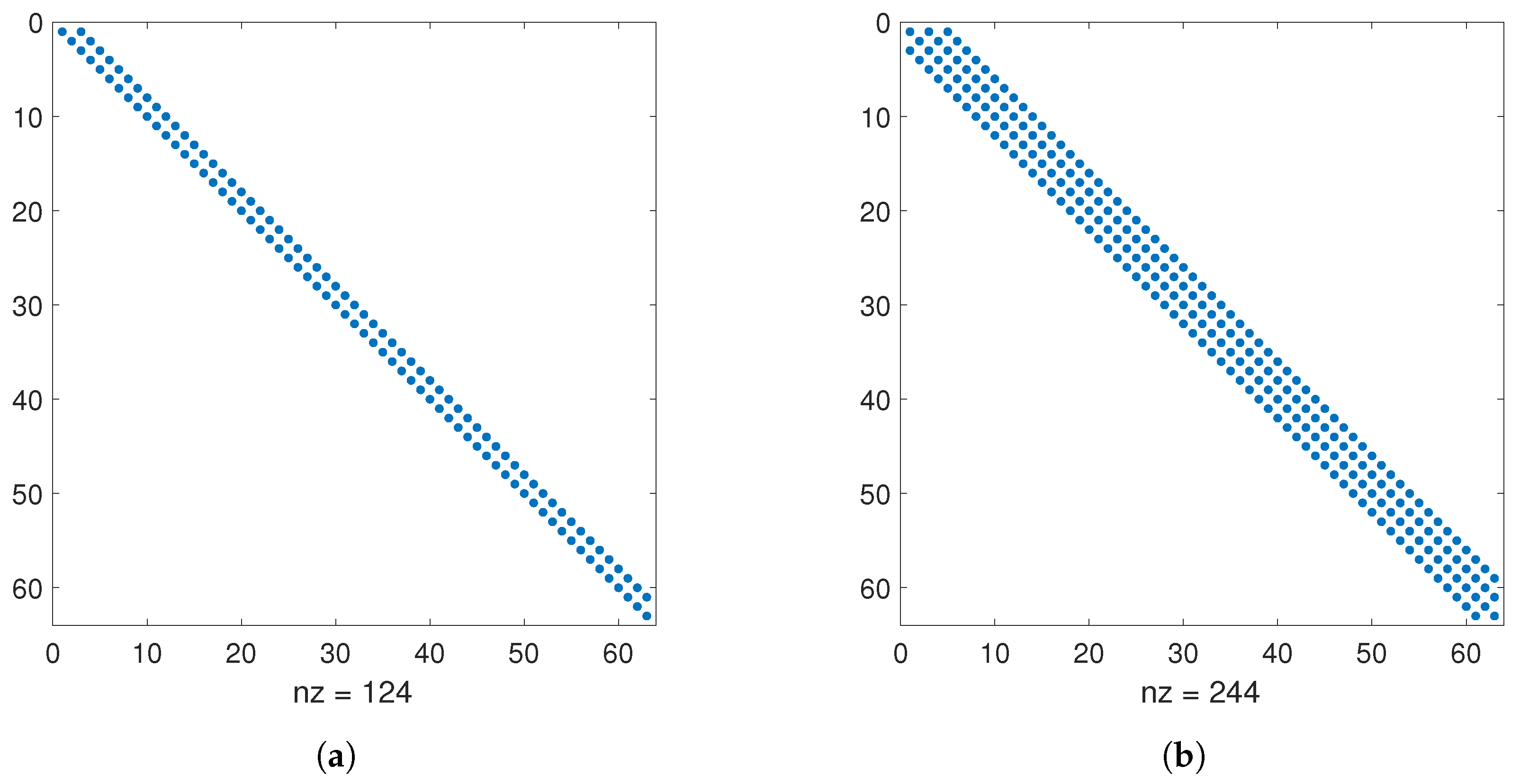If we set ${\mathbf{V}}^{\ast }=[{\mathbf{v}}_0^{\ast },{\mathbf{v}}_1^{\ast },\cdots ,{\mathbf{v}}_{M-2}^{\ast }]$ and $\mathbf{H}=[{\mathbf{h}}_0,{\mathbf{h}}_1,\cdots ,{\mathbf{h}}_{M-2}]$ and define the j-th diagonal element of $\mathbf{Q}$ as $q_j$, the j-th column of Equation (38) can be written as

$$({\tilde{\mathbf{A}}}_x+q_j{\tilde{\mathbf{C}}}_x){\mathbf{v}}_j^{\ast }={\mathbf{h}}_j$$

(39)

for $j=0,1,\cdots ,M-2$. The matrices ${\tilde{\mathbf{A}}}_x$ and ${\tilde{\mathbf{C}}}_x$ are bi-diagonal and quad-diagonal matrices, respectively, whose non-zero elements are presented in Figure 1. Due to the sparsity, solving Equation (39) for ${\mathbf{v}}_j^{\ast }$ can be performed efficiently with $\mathcal{O}(L)$ operations for all j. Once it is performed so that all elements of the matrix ${\mathbf{V}}^{\ast }$ are obtained, the matrix $\mathbf{V}$ can be computed from

$$\mathbf{V}={\mathbf{V}}^{\ast }{\mathbf{P}}^{-1}.$$

(40)

3.2. 3-D Poisson Equation

By following the same steps used in the 2-D problem, we can use the quasi-inverse matrix diagonalization method to 3-D PDEs. Here, we will explain the way to use the quasi-inverse matrix diagonalization method for 3-D problems, particularly applying it to solve a 3-D Poisson equation.

3.2.1. Quasi-Inverse Technique

We want to solve the 3-D Poisson equation with the following Dirichlet boundary conditions:

$$\begin{array}{c}\frac{{\partial }^{2}u}{\partial x^2}+\frac{{\partial }^{2}u}{\partial y^2}+\frac{{\partial }^{2}u}{\partial z^2}=f(x,y,z),(-1\le x\le 1,-1\le y\le 1,-1\le z\le 1)\\ u(\pm 1,y,z)=u(x,\pm 1,z)=u(x,y,\pm 1)=0.\end{array}$$

(41)

Definition 8.

In employing Chebyshev polynomials to solve PDEs, $u(x,y)$ and $f(x,y)$ are represented by the sums of Chebyshev coefficients multiplied by Chebyshev polynomials, defined as

$$u(x,y,z)=\sum _{l=0}^L\sum _{m=0}^M\sum _{n=0}^N{\widehat{u}}_{lmn}{T}_l(x)T_m(y)T_n(y)$$

(42)

and

$$f(x,y,z)=\sum _{l=0}^L\sum _{m=0}^M\sum _{n=0}^N{\widehat{f}}_{lmn}{T}_l(x)T_m(y)T_n(y)$$

(43)

where L, M and N are the highest Chebyshev modes in x, y, and z, respectively, and ${\widehat{u}}_{lmn}$ and ${\widehat{f}}_{lmn}$ are the $(l,m,n)$-th Chebyshev coefficients of $u(x,y,z)$ and $f(x,y,z)$, respectively.

In a matrix form, Equation (41) can be rewritten using the Kronecker product as

$$({\mathbf{D}}_x^2\otimes {\mathbf{I}}_y\otimes {\mathbf{I}}_z+{\mathbf{I}}_x\otimes {\mathbf{D}}_y^2\otimes {\mathbf{I}}_z+{\mathbf{I}}_x\otimes {\mathbf{I}}_y\otimes {\mathbf{D}}_z^2)\mathbf{u}=\mathbf{f},$$

(44)

where $\mathbf{u}$ and $\mathbf{f}$ are the $(L+1)(M+1)(N+1)\times 1$ arrays in which the j row components of those arrays are respectively equal to ${\widehat{u}}_{lmn}$ and ${\widehat{f}}_{lmn}$ where $j=(M+1)(N+1)l+(N+1)m+n$ for $l=0,1,\cdots ,L,$ $m=0,1,\cdots ,M$ and $n=0,1,\cdots ,N$. Multiplying to the left of Equation (44) by ${\mathbf{B}}_x\otimes {\mathbf{B}}_y\otimes {\mathbf{B}}_z$ gives

$$\left[{\mathbf{J}}_x\otimes {\mathbf{B}}_y\otimes {\mathbf{B}}_z+{\mathbf{B}}_x\otimes {\mathbf{J}}_y\otimes {\mathbf{B}}_z+{\mathbf{B}}_x\otimes {\mathbf{B}}_y\otimes {\mathbf{J}}_z\right]\mathbf{u}=({\mathbf{B}}_x\otimes {\mathbf{B}}_y\otimes {\mathbf{B}}_z)\mathbf{f}.$$

(45)

Definition 9.

When using the Chebyshev-Galerkin method, we approximate $u(x,y,z)$ with the Galerkin basis functions, with their coefficients as

$$u(x,y,z)=\sum _{l=0}^{L-2}\sum _{m=0}^{M-2}\sum _{n=0}^{N-2}{\widehat{v}}_{lmn}{\varphi }_l(x){\varphi }_m(y){\varphi }_n(z),$$

(46)

where ${\widehat{v}}_{lmn}$ is the $(l,m,n)$ mode coefficient of the Galerkin basis functions.

Remark 4.

By defining $\mathit{v}$ as the $(L-1)(M-1)(N-1)\times 1$ array in which the j row component is set to ${\widehat{v}}_{lmn}$ where $j=(M-1)(N-1)l+(N-1)m+n$ for $l=0,1,\cdots ,L-2,$ $m=0,1,\cdots ,M-2$ and $n=0,1,\cdots ,N-2$, the arrays $\mathit{u}$ and $\mathit{v}$ are associated by

$$\mathit{u}=({\mathit{S}}_x\otimes {\mathit{S}}_y\otimes {\mathit{S}}_z)\mathit{v}.$$

(47)

Substituting Equation (47) to Equation (45) and distributing the transformation matrix ${\mathbf{S}}_{\chi }$ in each direction produce

$$\left[({\mathbf{J}}_x{\mathbf{S}}_x)\otimes ({\mathbf{B}}_y{\mathbf{S}}_y)\otimes ({\mathbf{B}}_z{\mathbf{S}}_z)+({\mathbf{B}}_x{\mathbf{S}}_x)\otimes ({\mathbf{J}}_y{\mathbf{S}}_y)\otimes ({\mathbf{B}}_z{\mathbf{S}}_z)+({\mathbf{B}}_x{\mathbf{S}}_x)\otimes ({\mathbf{B}}_y{\mathbf{S}}_y)\otimes ({\mathbf{J}}_z{\mathbf{S}}_z)\right]\mathbf{v}=({\mathbf{B}}_x\otimes {\mathbf{B}}_y\otimes {\mathbf{B}}_z)\mathbf{f}.$$

(48)

As we defined in the solution of the 2-D Poisson equation, use notations of ${\mathbf{A}}_{\chi }={\mathbf{J}}_{\chi }{\mathbf{S}}_{\chi }$ and ${\mathbf{C}}_{\chi }={\mathbf{B}}_{\chi }{\mathbf{S}}_{\chi }$ for $\chi =x,y$ and z. Then, Equation (49) can be rewritten as

$$\left[{\mathbf{A}}_x\otimes {\mathbf{C}}_y\otimes {\mathbf{C}}_z+{\mathbf{C}}_x\otimes {\mathbf{A}}_y\otimes {\mathbf{C}}_z+{\mathbf{C}}_x\otimes {\mathbf{C}}_y\otimes {\mathbf{A}}_z\right]\mathbf{v}=({\mathbf{B}}_x\otimes {\mathbf{B}}_y\otimes {\mathbf{B}}_z)\mathbf{f}.$$

(49)

At each matrix in Equation (49), all elements in the top two rows are zeros because those places are discarded to impose boundary conditions. Erasing those rows and using the symbol tilde to represent the deleted top two rows of given matrices give

$$\left[{\tilde{\mathbf{A}}}_x\otimes {\tilde{\mathbf{C}}}_y\otimes {\tilde{\mathbf{C}}}_z+{\tilde{\mathbf{C}}}_x\otimes {\tilde{\mathbf{A}}}_y\otimes {\tilde{\mathbf{C}}}_z+{\tilde{\mathbf{C}}}_x\otimes {\tilde{\mathbf{C}}}_y\otimes {\tilde{\mathbf{A}}}_z\right]\mathbf{v}=({\tilde{\mathbf{B}}}_x\otimes {\tilde{\mathbf{B}}}_y\otimes {\tilde{\mathbf{B}}}_z)\mathbf{f}.$$

(50)

For simplicity, define ${\tilde{\mathbf{E}}}_{xy}={\tilde{\mathbf{A}}}_x\otimes {\tilde{\mathbf{C}}}_y+{\tilde{\mathbf{C}}}_x\otimes {\tilde{\mathbf{A}}}_y$, ${\tilde{\mathbf{C}}}_{xy}={\tilde{\mathbf{C}}}_x\otimes {\tilde{\mathbf{C}}}_y$ and ${\tilde{\mathbf{B}}}_{xy}={\tilde{\mathbf{B}}}_x\otimes {\tilde{\mathbf{B}}}_y$, then Equation (50) can be simplified as

$$\left[{\tilde{\mathbf{C}}}_{xy}\otimes {\tilde{\mathbf{A}}}_z+{\tilde{\mathbf{E}}}_{xy}\otimes {\tilde{\mathbf{C}}}_z\right]\mathbf{v}=({\tilde{\mathbf{B}}}_{xy}\otimes {\tilde{\mathbf{B}}}_z)\mathbf{f}.$$

(51)

3.2.2. Matrix Diagonalization Method

Decomposition of Equation (51) can be performed by using the same matrix diagonalization steps used in the 2-D Poisson equation. However, here we want to briefly describe the procedure again to clearly show how the equation is diagonalized and solved efficiently in 3-D problems.

We reshape the array $\mathbf{v}$ and $\mathbf{f}$ to the $(L-1)(M-1)\times (N-1)$ matrix and $(L+1)(M+1)\times (N+1)$ matrix and define them as $\mathbf{V}$ and $\mathbf{F}$, respectively. With these matrices, we can rewrite Equation (51) as

$${\tilde{\mathbf{C}}}_{xy}\mathbf{V}{\tilde{\mathbf{A}}}_z^T+{\tilde{\mathbf{E}}}_{xy}\mathbf{V}{\tilde{\mathbf{C}}}_z^T={\tilde{\mathbf{B}}}_{xy}\mathbf{F}{\tilde{\mathbf{B}}}_z^T.$$

(52)

Let us multiply on the right by ${\tilde{\mathbf{A}}}_z^{-T}$ to Equation (52)

$${\tilde{\mathbf{C}}}_{xy}\mathbf{V}+{\tilde{\mathbf{E}}}_{xy}\mathbf{V}{\tilde{\mathbf{C}}}_z^T{\tilde{\mathbf{A}}}_z^{-T}={\tilde{\mathbf{B}}}_{xy}\mathbf{F}{\tilde{\mathbf{B}}}_z^T{\tilde{\mathbf{A}}}_z^{-T}.$$

(53)

and decompose ${\tilde{\mathbf{C}}}_z^T{\tilde{\mathbf{A}}}_z^{-T}$ as

$${\tilde{\mathbf{C}}}_z^T{\tilde{\mathbf{A}}}_z^{-T}=\mathbf{P}\mathbf{Q}{\mathbf{P}}^{-1},$$

(54)

where $\mathbf{P}$ and $\mathbf{Q}$ are the eigenvector matrix and diagonal eigenvalue matrix of ${\tilde{\mathbf{C}}}_z^T{\tilde{\mathbf{A}}}_z^{-T}$, respectively. Then, after substituting Equation (54) to Equation (53) and multiplying on the right by $\mathbf{P}$, if we define $\mathbf{W}=\mathbf{V}\mathbf{P}$ and $\mathbf{G}={\tilde{\mathbf{B}}}_{xy}\mathbf{F}{\tilde{\mathbf{B}}}_z^T{\tilde{\mathbf{A}}}_z^{-T}\mathbf{P}$, it is possible to obtain

$$({\tilde{\mathbf{C}}}_{xy}+q_k{\tilde{\mathbf{E}}}_{xy}){\mathbf{w}}_k={\mathbf{g}}_k$$

(55)

for $k=0,1,\cdots ,N-2$ where the $q_k$ is the k-th diagonal element of $\mathbf{Q}$, and $\mathbf{W}$ and $\mathbf{G}$ are set as $\mathbf{W}=[{\mathbf{w}}_0,{\mathbf{w}}_1,\cdots ,{\mathbf{w}}_{N-2}]$ and $\mathbf{G}=[{\mathbf{g}}_0,{\mathbf{g}}_1,\cdots ,{\mathbf{g}}_{N-2}]$, respectively.

Equation (55) is decoupled in z direction but still coupled in x and y directions. To decouple it completely in all directions, based on the definition of ${\tilde{\mathbf{C}}}_{xy}$ and ${\tilde{\mathbf{E}}}_{xy}$, Equation (55) can be expanded as

$$\left[({\tilde{\mathbf{C}}}_x+q_k{\tilde{\mathbf{A}}}_x)\otimes {\tilde{\mathbf{C}}}_y+q_k{\tilde{\mathbf{C}}}_x\otimes {\tilde{\mathbf{A}}}_y\right]{\mathbf{w}}_k={\mathbf{g}}_k.$$

(56)

Again, let’s reshape $(L-1)(M-1)\times 1$ arrays ${\mathbf{w}}_k$ and ${\mathbf{g}}_k$ to $(L-1)\times (M-1)$ matrices and refer those matrices as $\mathbf{Z}(k)$ and $\mathbf{H}(k)$. Note that the index k in the parenthesis here is used to clearly show that those matrices are a function of k so that the matrices’ entries are changed when k is changed. Defining ${\mathbf{K}}_x(k)$ =${\tilde{\mathbf{C}}}_x+q_k{\tilde{\mathbf{A}}}_x$ allows Equation (56) to be rewritten as

$${\mathbf{K}}_x\mathbf{Z}(k){\tilde{\mathbf{C}}}_y^T+q_k{\tilde{\mathbf{C}}}_x\mathbf{Z}(k){\tilde{\mathbf{A}}}_y^T=\mathbf{H}(k).$$

(57)

At each k, Equation (57) is the 2-D coupled equation. This is the same type of equation as Equation (35), and therefore the $\mathbf{Z}(k)$ can be efficiently solved by applying the matrix diagonalization method once again to separate coupled modes in x and y directions. To do this, after multiplying on the right by ${\tilde{\mathbf{C}}}_y^{-T}$ to Equation (57), decompose ${\tilde{\mathbf{A}}}_y^T{\mathbf{C}}_y^{-T}=\mathbf{R}\Lambda {\mathbf{R}}^{-1}$ where $\mathbf{R}$ and $\Lambda$ are the eigenvector matrix and diagonal eigenvalue matrix of ${\tilde{\mathbf{A}}}_y^T{\mathbf{C}}_y^{-T}$, respectively. After that, if we multiply on the right by $\mathbf{R}$ and set $\mathbf{Y}(k)=\mathbf{Z}(k)\mathbf{R}$ and $\mathbf{S}(k)=\mathbf{H}(k){\mathbf{C}}_y^{-T}\mathbf{R}$, then we can get

$$({\mathbf{K}}_x+q_k{\lambda }_j{\tilde{\mathbf{C}}}_x){\mathbf{y}}_j(k)={\mathbf{s}}_j(k).$$

(58)

Here, the ${\lambda }_j$ is the j-th diagonal element of $\Lambda$, and $\mathbf{Y}(k)$ and $\mathbf{S}(k)$ are set to $\mathbf{Y}(k)=[{\mathbf{y}}_0(k),{\mathbf{y}}_0(k),\cdots ,{\mathbf{y}}_{M-2}(k)]$ and $\mathbf{S}(k)=[{\mathbf{s}}_0(k),{\mathbf{s}}_1(k),\cdots ,{\mathbf{s}}_{M-2}(k)]$. For each k and j, Equation (58) can be solved for ${\mathbf{y}}_j(k)$ in $\mathcal{O}(L)$ operations.

4. Numerical Examples

In this section, our quasi-inverse matrix diagonalization method is applied to several 2-D and 3-D PDEs, and the numerical results are presented. The numbers of Chebyshev modes to discretize solutions at each spatial direction do not need to be identical. Nonetheless, we use the same numbers of Chebyshev modes N at each spatial direction in all test problems for simplicity. Numerical codes are implemented in MATLAB and operated using a 16 GB-RAM Macbook Pro with a 2.3 GHz quad-core Intel Core i7 processor. For matrix diagonalization, MATLAB’s built-in function “eig” is used to compute the matrix’s eigenvalues and eigenvectors. For inverse matrix calculation, we use MATLAB’s backslash operator.

4.1. Multi-Dimensional Poisson Equation

The n-dimensional Poisson equations described in Section 3 are solved using the quasi-inverse matrix diagonalization method for $n=2$ and 3

$$\Delta u(\underline{x})=f(\underline{x}),u=0\mathrm{on}\Gamma$$

(59)

where $\Gamma$ is the boundary of the rectangular domain. As a test example, we define $f(\underline{x})$ as

$$f(\underline{x})=-n(4{\pi }^2)\prod _{i=1}^{n}sin(2\pi x_i).$$

(60)

Note that we use coordinates $x_1$ and $x_2$ in the 2-D problem and $x_1$, $x_2$, and $x_3$ in the 3-D problem. Then, the exact solution of Equation (59) becomes

$$u(\underline{x})=\prod _{i=1}^{n}sin(2\pi x_i).$$

(61)

This test problem is solved using the quasi-inverse technique, matrix diagonalization method, and quasi-inverse matrix diagonalization method. The accuracy of numerical solutions obtained with these three methods is presented in

Table 1. Errors of numerical solutions of 2-D and 3-D Poisson equations as a function of unknowns in 1-D. The numerical solutions are computed using QI, MD, and OIMD methods where QI, MD, and QIMD stand for Quasi-Inverse, Matrix Diagonalization, and Quasi-Inverse Matrix Diagonalization, respectively. All methods show a similar order of accuracy and reach spectral accuracy at $N=32$.

Method	N	Error (2-D)	Error (3-D)
QI method	8	$1.68\times {10}^{-1}$	$1.87\times {10}^{-2}$
	16	$1.75\times {10}^{-6}$	$2.83\times {10}^{-6}$
	24	$4.36\times {10}^{-13}$	$7.31\times {10}^{-13}$
	32	$6.39\times {10}^{-16}$	$1.58\times {10}^{-15}$
MD method	8	$1.68\times {10}^{-1}$	$1.87\times {10}^{-2}$
	16	$1.75\times {10}^{-6}$	$2.83\times {10}^{-6}$
	24	$4.36\times {10}^{-13}$	$7.31\times {10}^{-13}$
	32	$1.75\times {10}^{-15}$	$3.41\times {10}^{-15}$
QIMD method	8	$1.68\times {10}^{-1}$	$1.87\times {10}^{-2}$
	16	$1.75\times {10}^{-6}$	$2.83\times {10}^{-7}$
	24	$4.36\times {10}^{-13}$	$7.31\times {10}^{-13}$
	32	$1.43\times {10}^{-15}$	$3.62\times {10}^{-15}$

as a function of N where the accuracy is computed by the relative ${\mathrm{L}}_2$-norm error between the exact and numerical solutions, defined as

$$\mathrm{Error}=\frac{\left|\right|u-u_{ext}{\left|\right|}_2}{\left|\right|u_{ext}{\left|\right|}_2},$$

(62)

where ${\left|\right|\left|\right|}_2$ indicates the ${\mathrm{L}}_2$-norm, and u and $u_{ext}$ are the numerical and exact solutions, respectively. In both 2-D and 3-D problems, three methods show a similar order of accuracy, which is identical until $N=24$. At $N=32$, all numerical solutions encounter machine accuracy (∼10${}^{-16}$) in double precision.

At high N, errors of numerical solutions obtained from the spectral method using Chebyshev polynomials can increase because the system of equation tends to be ill-conditioned as N increases. To be a good spectral method, the error of numerical solutions at high N should be retained near the machine accuracy and should not rise as N increases. In this aspect, to further check the error and robustness of the proposed method, we solve the Poisson problem with high N up to $N=1024$ in 2-D and $N=256$ in 3-D and measure the errors of numerical solutions of the proposed method as a function of N. We present the results of this experiment in Figure 2. As shown in the figure, even at high N, the errors of numerical solutions of the proposed method retain the order of ${10}^{-15}$, showing high accuracy and robustness of the proposed method.

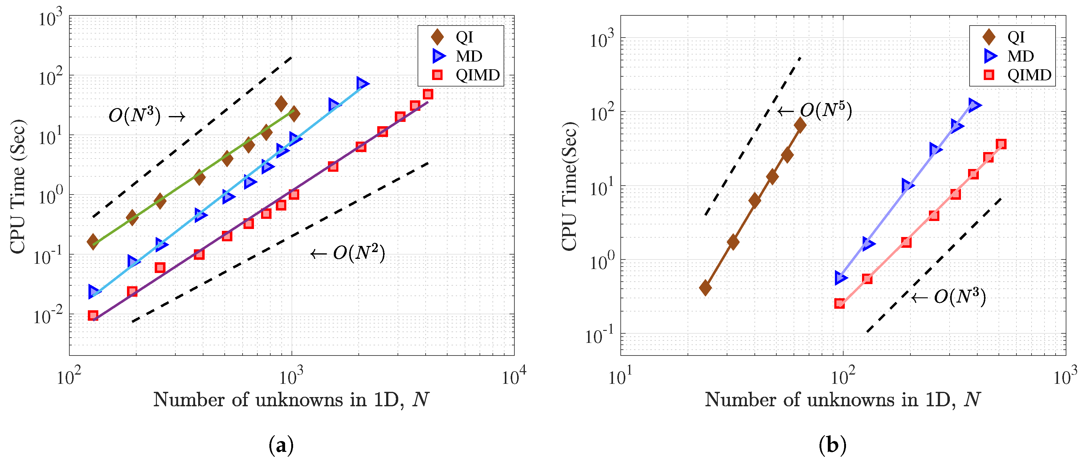
Figure 3 shows the CPU time of the quasi-inverse, matrix diagonalization, and quasi-inverse matrix diagonalization methods in solving 2-D and 3-D Poisson equations as a function of N as a log-log scale. Then, we know that the slope of each method’s data in the figure indicates the operation complexity of the corresponding method. To calculate slopes, the date are fitted using the best linear regression by $t=\exp (m\ln N+b)$ where t is CPU time, and m and b are the coefficients of best linear regression. The results of the best regression are presented in

Table 2. CPU time (t) and the number of unknowns in 1-D (N) are associated using the best linear regression in the log-log scale by $t=\exp (mlnN+b)$. Values of m, b and $r^2$ of the Quasi-Inverse (QI), Matrix Diagonalization(MD) and Quasi-Inverse Matrix Diagonalization (QIMD) methods in solving 2-D and 3-D Poisson equations are presented where $r^2$ here is the r-squared value of the best linear regression.

Method	2-D			3-D
	$\mathit{m}$	$\mathit{b}$	${\mathit{r}}^{\mathbf{2}}$	$\mathit{m}$	$\mathit{b}$	${\mathit{r}}^{\mathbf{2}}$
QI method	2.498	$-14.069$	0.8857	5.055	$-16.043$	0.9899
MD method	2.890	$-17.936$	0.9833	3.934	$-18.511$	0.9922
QIMD method	2.431	$-16.655$	0.9669	2.973	$-15.033$	0.9951

where $r^2$ is the r-squared value of the best linear regression.

In solving the 2-D Poisson equation, we observe that the operation complexity of the matrix diagonalization method is highest among the three methods, while the other two methods show similar operation complexity. However, actual CPU time of the quasi-inverse matrix diagonalization method is more than 10 times shorter than the quasi-inverse method. These observations indicate that reduction of operation complexity comes from the quasi-inverse technique’s ability to make the equations of systems sparse, rather than from the matrix diagonalization technique. However, the matrix diagonalization technique is still able to help reduce CPU times by decreasing the actual number of calculations, even though the two methods have the same order of operation complexity.

In solving the 3-D Poisson equation, as Julien and Waston claimed in [13], the operation complexity of the quasi-inverse technique is approximately $\mathcal{O}(N^5)$. In the matrix diagonalization method, the operation complexity approximately increases from $\mathcal{O}(N^3)$ to $\mathcal{O}(N^4)$ as dimensionality of the Poisson equation rises from 2-D to 3-D. This is because the bottleneck of the matrix diagonalization method in solving the Poisson equation is computing ${\mathbf{v}}_i$ from the dense matrix, which requires about $\mathcal{O}(N^2)$ operations per calculation, and repetition of this calculation increases from N to $N^2$ times. When using the quasi-inverse matrix diagonalization method to solve the 3-D problem, the most time consuming step is also computing ${\mathbf{v}}_i$, but the left-hand side matrix $({\mathbf{K}}_x+q_i{\lambda }_j{\tilde{\mathbf{C}}}_x)$ in Equation (58) is sparse where the bandwidth is four, and therefore ${\mathbf{v}}_i$ can be solved in $\mathcal{O}(N)$ operations. Because this calculation is repeated $N^2$ times in the 3-D problem, the total operation complexity of the quasi-inverse matrix diagonalization method becomes $\mathcal{O}(N^3)$ as shown in Table 2.

4.2. Two-Dimensional Poisson Equation with No Analytic Solution

The next numerical example is a 2-D Poisson equation with the complicated forcing term. That is, we solve the same problem described in Section 3 in 2-D but with the forcing term

$$f(x)=\frac{20sin(\pi x)sin(\pi y)e^{xy}}{\sqrt{1+tanh{(x)}^2+tanh{(y)}^2}}.$$

(63)

Note that analytic solutions cannot be found for this Poisson equation. The problem is solved using the quasi-inverse matrix diagonalization method by changing the number of unknowns so $N=16,32,64,128,256,512$, and 1024.

Figure 4 shows the values of the forcing term $f(x,y)$ in Figure 4a and the numerical solution of the problem $u(x,y)$ at $N=128$ in Figure 4b. To check the accuracy of the quasi-inverse matrix diagonalization method in solving this problem, we compute the numerical errors of the problem. Because no exact solution of the problem is available, we treat the numerical solution at $N=1024$ as the most accurate solution and compare the other numerical solutions with it. Therefore, the error here indicates the relative difference between the numerical solutions obtained at $N<1024$ and the numerical solution obtained at $N=1024$ in a sense of the ${\mathrm{L}}_2$ norm. We present the values of the errors as a function of N as a log-log scale in Figure 5. As N increases, the error decreases exponentially, which shows spectral accuracy of our method, as expected.

4.3. Coupled Two-Dimensional Helmholtz Equation

We apply the quasi-inverse matrix diagonalization method to 2-D coupled Helmholtz equations and compared the numerical results with the ones obtained from the quasi-inverse technique. We consider the following coupled equations with Dirichlet boundary conditions

$$\begin{array}{cc}\hfill \Delta u_1& +k_1{u}_2=f_1(x,y)\hfill \\ \hfill k_2{u}_1& +\Delta u_2=f_2(x,y)\hfill \\ \hfill u_1(x,y)=0,& u_2(x,y)=0\mathrm{on}\Gamma \hfill \end{array}$$

(64)

where $k_1$ and $k_2$ are constant numbers. As a test problem, the functions $f_1(x,y)$ and $f_2(x,y)$ are assumed as

$$\begin{array}{cc}\hfill f_1(x,y)& =-2sin(\pi x)sin(\pi y)+\frac{k_1}{{\pi }^2}\left(1+cos(\pi x)+cos(\pi y)+cos(\pi x)cos(\pi y)\right)\hfill \\ \hfill f_2(x,y)& =-cos(\pi x)-cos(\pi y)-2cos(\pi x)cos(\pi y)+\frac{k_2}{{\pi }^2}sin(\pi x)sin(\pi y).\hfill \end{array}$$

(65)

Then, the exact solutions of Equation (64) are

$$u_1(x,y)=\frac{1}{{\pi }^2}sin(\pi x)sin(\pi y),u_2(x,y)=\frac{1}{{\pi }^2}\left(1+cos(\pi x)\right)\left(1+cos(\pi y)\right).$$

(66)

The numerical solutions $u_1(x,y)$ and $u_2(x,y)$ are defined by using Chebyshev polynomials and Galerkin basis functions as

$$\begin{array}{cc}\hfill u_1(x,y)& =\sum _{l=0}^L\sum _{m=0}^M{({\widehat{u}}_1)}_{lm}{T}_l(x)T_m(y)=\sum _{l=0}^{L-2}\sum _{m=0}^{M-2}{({\widehat{v}}_1)}_{lm}{\varphi }_l(x){\varphi }_m(y)\hfill \\ \hfill u_2(x,y)& =\sum _{l=0}^L\sum _{m=0}^M{({\widehat{u}}_2)}_{lm}{T}_l(x)T_m(y)=\sum _{l=0}^{L-2}\sum _{m=0}^{M-2}{({\widehat{v}}_2)}_{lm}{\varphi }_l(x){\varphi }_m(y)\hfill \end{array}$$

(67)

and $f_1(x,y)$ and $f_2(x,y)$ are defined using Chebyshev polynomials as

$$\begin{array}{cc}\hfill f_1(x,y)& =\sum _{l=0}^L\sum _{m=0}^M{({\widehat{f}}_1)}_{lm}{\varphi }_l(x){\varphi }_m(y)\hfill \\ \hfill f_2(x,y)& =\sum _{l=0}^L\sum _{m=0}^M{({\widehat{f}}_2)}_{lm}{\varphi }_l(x){\varphi }_m(y).\hfill \end{array}$$

(68)

For $k=1$ and 2, define two $(L-1)(M-1)\times 1$ arrays as ${\mathbf{v}}_k$ and ${\mathbf{f}}_k$ in which the j-th entries are respectively equal to ${({\widehat{v}}_k)}_{lm}$ and ${({\widehat{f}}_k)}_{lm}$ where $j=(M-1)l+m$ for $l=0,1,\cdots ,L-2$ and $m=0,1,\cdots ,M-2$. This allows us to express Equation (64) in a matrix form as

$$\begin{array}{c}\hfill \left[({\mathbf{J}}_x{\mathbf{S}}_x)\otimes ({\mathbf{B}}_y{\mathbf{S}}_y)+({\mathbf{B}}_x{\mathbf{S}}_x)\otimes ({\mathbf{J}}_y{\mathbf{S}}_y)\right]{\mathbf{v}}_1+k_1\left[({\mathbf{B}}_x{\mathbf{S}}_x)\otimes ({\mathbf{B}}_y{\mathbf{S}}_y)\right]{\mathbf{v}}_2=({\mathbf{B}}_x\otimes {\mathbf{B}}_y){\mathbf{f}}_1\\ \hfill \left[({\mathbf{J}}_x{\mathbf{S}}_x)\otimes ({\mathbf{B}}_y{\mathbf{S}}_y)+({\mathbf{B}}_x{\mathbf{S}}_x)\otimes ({\mathbf{J}}_{\mathbf{y}}{\mathbf{S}}_y)\right]{\mathbf{v}}_2+k_2\left[({\mathbf{B}}_x{\mathbf{S}}_x)\otimes ({\mathbf{B}}_y{\mathbf{S}}_y)\right]{\mathbf{v}}_1=({\mathbf{B}}_x\otimes {\mathbf{B}}_y){\mathbf{f}}_2.\end{array}$$

(69)

To make Equation (69) simple, rewrite ${\mathbf{J}}_{\chi }{\mathbf{S}}_{\chi }$ and ${\mathbf{B}}_{\chi }{\mathbf{S}}_{\chi }$ as ${\mathbf{A}}_{\chi }$ and ${\mathbf{C}}_{\chi }$, respectively, then

$$\begin{array}{c}\hfill \left({\mathbf{A}}_x\otimes {\mathbf{C}}_y+{\mathbf{C}}_x\otimes {\mathbf{A}}_y\right){\mathbf{v}}_1+k_1\left({\mathbf{C}}_x\otimes {\mathbf{C}}_y\right){\mathbf{v}}_2=({\mathbf{B}}_x\otimes {\mathbf{B}}_y){\mathbf{f}}_1\\ \hfill \left({\mathbf{A}}_x\otimes {\mathbf{C}}_y+{\mathbf{C}}_x\otimes {\mathbf{A}}_y\right){\mathbf{v}}_2+k_2\left({\mathbf{C}}_x\otimes {\mathbf{C}}_y\right){\mathbf{v}}_1=({\mathbf{B}}_x\otimes {\mathbf{B}}_y){\mathbf{f}}_2.\end{array}$$

(70)

Erasing the top two rows of the matrices in Equation (70) as we did in solving the multi-dimensional Poisson equations gives

$$\begin{array}{c}\hfill \left({\tilde{\mathbf{A}}}_x\otimes {\tilde{\mathbf{C}}}_y+{\tilde{\mathbf{C}}}_x\otimes {\tilde{\mathbf{A}}}_y\right){\mathbf{v}}_1+k_1\left({\tilde{\mathbf{C}}}_x\otimes {\tilde{\mathbf{C}}}_y\right){\mathbf{v}}_2=({\tilde{\mathbf{B}}}_x\otimes {\tilde{\mathbf{B}}}_y){\mathbf{f}}_1\\ \hfill \left({\tilde{\mathbf{A}}}_x\otimes {\tilde{\mathbf{C}}}_y+{\tilde{\mathbf{C}}}_x\otimes {\tilde{\mathbf{A}}}_y\right){\mathbf{v}}_2+k_2\left({\tilde{\mathbf{C}}}_x\otimes {\tilde{\mathbf{C}}}_y\right){\mathbf{v}}_1=({\tilde{\mathbf{B}}}_x\otimes {\tilde{\mathbf{B}}}_y){\mathbf{f}}_2,\end{array}$$

(71)

where the symbol tilde is defined as before. We want to combine two equations in Equation (71). To do this, define $\mathbf{v}=[{\mathbf{v}}_1;{\mathbf{v}}_2]$ and ${\mathbf{J}}_i$ as

$${\mathbf{J}}_i=\left[\begin{array}{cc}{\alpha }_1& {\alpha }_2\\ {\alpha }_3& {\alpha }_4\end{array}\right],$$

where ${\alpha }_j=1$ if $i=j$, otherwise 0. Then, two equations in Equation (71) can be combined as

$$\begin{array}{cc}\hfill [({\tilde{\mathbf{A}}}_x\otimes {\tilde{\mathbf{C}}}_y+& {\tilde{\mathbf{C}}}_x\otimes {\tilde{\mathbf{A}}}_y)\otimes {\mathbf{J}}_1]\mathbf{v}+k_1\left[({\tilde{\mathbf{C}}}_x\otimes {\tilde{\mathbf{C}}}_y)\otimes {\mathbf{J}}_2\right]\mathbf{v}+\left[({\tilde{\mathbf{A}}}_x\otimes {\tilde{\mathbf{C}}}_y+{\tilde{\mathbf{C}}}_x\otimes {\tilde{\mathbf{A}}}_y)\otimes {\mathbf{J}}_4\right]\mathbf{v}\hfill \\ & +k_2\left[({\tilde{\mathbf{C}}}_x\otimes {\tilde{\mathbf{C}}}_y)\otimes {\mathbf{J}}_3\right]\mathbf{v}=({\tilde{\mathbf{B}}}_x\otimes {\tilde{\mathbf{B}}}_y\otimes {\mathbf{J}}_1)\mathbf{f}+({\tilde{\mathbf{B}}}_x\otimes {\tilde{\mathbf{B}}}_y\otimes {\mathbf{J}}_4)\mathbf{f}.\hfill \end{array}$$

(72)

By rearranging the terms, Equation (72) can be rewritten as

$$\begin{array}{c}\hfill ({\tilde{\mathbf{E}}}_{xy}\otimes ({\mathbf{J}}_1+{\mathbf{J}}_4))\mathbf{v}+({\tilde{\mathbf{C}}}_{xy}\otimes (k_1{\mathbf{J}}_2+k_2{\mathbf{J}}_3))\mathbf{v}=({\tilde{\mathbf{B}}}_{xy}\otimes ({\mathbf{J}}_1+{\mathbf{J}}_4))\mathbf{f},\end{array}$$

(73)

where ${\tilde{\mathbf{E}}}_{xy}={\tilde{\mathbf{A}}}_x\otimes {\tilde{\mathbf{C}}}_y+{\tilde{\mathbf{C}}}_x\otimes {\tilde{\mathbf{A}}}_y$, ${\tilde{\mathbf{C}}}_{xy}={\tilde{\mathbf{C}}}_x\otimes {\tilde{\mathbf{C}}}_y$ and ${\tilde{\mathbf{B}}}_{xy}={\tilde{\mathbf{B}}}_x\otimes {\tilde{\mathbf{B}}}_y$ as defined in Section 3.2. Because Equations (73) and (51) are the same types of equations, Equation (73) can be solved for $\mathbf{v}$ by following the same steps as solving 3-D PDEs described in Section 3.2.

We tested coupled 2-D Helmholtz equations at $k_1=0.7$ and $k_2=1.1$. When N is 32, 64, 128, 256, and 512, the L-infinite errors between the numerical and exact solutions and CPU times are computed using the quasi-inverse and quasi-inverse matrix diagonalization methods, and the results are presented in

Table 3. Results of solving the coupled Helmholtz equations using the Quasi-Inverse (QI) and Quasi-Inverse Matrix Diagonalization (QIMD) methods with respect to accuracy and CPU times. Although both methods show the similar order of accuracy as a function of N, the CPU times of the QIMD method are much less than the ones of the QI method, showing the high efficiency of the QIMD method.

N	QI Method			QIMD Method
	Error $({\mathit{u}}_1)$	Error $({\mathit{u}}_2)$	CPU Time (s)	Error $({\mathit{u}}_1)$	Error $({\mathit{u}}_2)$	CPU Time (s)
32	$5.94\times {10}^{-16}$	$3.10\times {10}^{-16}$	$2.94\times {10}^{-2}$	$9.19\times {10}^{-16}$	$4.94\times {10}^{-16}$	$3.98\times {10}^{-2}$
64	$5.78\times {10}^{-16}$	$4.48\times {10}^{-16}$	$1.71\times {10}^{-1}$	$1.25\times {10}^{-15}$	$7.85\times {10}^{-16}$	$9.40\times {10}^{-2}$
128	$5.78\times {10}^{-16}$	$4.48\times {10}^{-16}$	$1.29\times {10}^0$	$1.37\times {10}^{-15}$	$7.06\times {10}^{-16}$	$2.14\times {10}^{-1}$
256	$4.66\times {10}^{-16}$	$4.58\times {10}^{-16}$	$6.47\times {10}^0$	$1.12\times {10}^{-15}$	$6.45\times {10}^{-16}$	$5.89\times {10}^{-1}$
512	$5.58\times {10}^{-16}$	$4.48\times {10}^{-16}$	$3.26\times {10}^1$	$1.49\times {10}^{-15}$	$8.75\times {10}^{-16}$	$1.75\times {10}^0$

. In both cases, the same order of high accuracy is obtained for all N. In terms of CPU time, similar to the multi-dimensional Poisson equation problems, the latter method is much faster than the former method, especially when N is high, showing the efficiency of our quasi-inverse matrix diagonalization method.

4.4. Stokes Problem

As a last text problem, a 3-D Stokes problem is solved using our quasi-inverse matrix diagonalization method. The Stokes problem we solved is

$$\begin{array}{c}\mu (\frac{{\partial }^{2}u}{\partial x^2}+\frac{{\partial }^{2}u}{\partial y^2}+\frac{{\partial }^{2}u}{\partial z^2})-\frac{\partial p}{\partial x}+f_x=0\\ \mu (\frac{{\partial }^{2}v}{\partial x^2}+\frac{{\partial }^{2}v}{\partial y^2}+\frac{{\partial }^{2}v}{\partial z^2})-\frac{\partial p}{\partial y}+f_y=0\\ \mu (\frac{{\partial }^{2}w}{\partial x^2}+\frac{{\partial }^{2}w}{\partial y^2}+\frac{{\partial }^{2}w}{\partial z^2})-\frac{\partial p}{\partial z}+f_z=0\\ \frac{\partial u}{\partial x}+\frac{\partial v}{\partial y}+\frac{\partial w}{\partial z}=0\end{array}$$

(74)

with the boundary conditions $u=v=w=p=0\mathrm{on}\Gamma$ where $\Gamma$ is the boundary of the rectangular domain. In the problem, we set the body force terms $f_x,f_y$ and $f_z$ in Equation (74) as

$$\begin{array}{cc}\hfill f_x& =-4\pi (e^{cos(2\pi x)}-e)sin(2\pi y)sin(2\pi z)\hfill \\ \hfill f_y& =\pi e^{cos(2\pi x)}sin(2\pi x)sin(2\pi z)g(x,y)\hfill \\ \hfill f_z& =\pi e^{cos(2\pi x)}sin(2\pi x)cos(2\pi y)g(x,z),\hfill \end{array}$$

(75)

where $g(x,y)=\left[{cos}^2(2\pi x)+3cos(2\pi x)+1\right]\left[cos(2\pi y)-1\right]+3cos(2\pi y)$ and $\mu =1$. Then, the exact solutions of this Stokes problem are given by

$$\begin{array}{cc}\hfill u& =-\frac{1}{2\pi }\left(e^{cos(2\pi x)}-e\right)sin(2\pi y)sin(2\pi z)\hfill \\ \hfill v& =\frac{1}{4\pi }{e}^{cos(2\pi x)}sin(2\pi x)sin(2\pi z)(cos(2\pi y)-1)\hfill \\ \hfill w& =\frac{1}{4\pi }{e}^{cos(2\pi x)}sin(2\pi x)sin(2\pi y)(cos(2\pi z)-1)\hfill \\ \hfill p& =e^{cos(2\pi x)}sin(2\pi x)sin(2\pi y)sin(2\pi z).\hfill \end{array}$$

(76)

The accuracy of numerical solutions of $u,v,w$, and p obtained using the quasi-inverse matrix diagonalization method is presented in Figure 6. The errors decay slower than the ones tested in the previous examples, but all of them show spectral convergence that reached machine accuracy around $N=90$. Figure 7 shows the CPU time of the Stokes problem in a log-log scale as a function of N. When the best linear regression of the data is implemented, the slope of this graph is 2.884, approximately showing $\mathcal{O}(N^3)$ operation complexity of the 3-D Stokes problem as expected.

5. Conclusions

A new efficient way of solving multi-dimensional linear PDEs spectrally using Chebyshev polynomials called the quasi-inverse matrix diagonalization method is presented in this paper. In this method, we discretize numerical solutions in spaces using the Chebyshev-Galerkin basis functions, which automatically obey the boundary conditions of the PDEs. Then, the quasi-inverse technique is used to construct sparse differential operators for the Chebyshev-Galerkin basis functions, and the matrix diagonalization technique is applied to further facilitate computations by decoupling the modes in spatial directions. It is proved that the proposed method is highly efficient compared to other current methods when applying it on the test problems. The proposed method is especially fast in computing 3-D linear PDEs. We show that the operation complexity of the proposed method in solving 3-D linear PDEs is approximately $\mathcal{O}(N^3)$ when tested with the numerical examples in this paper (tested up to $N=512$), suggesting the possibility of handling 3-D linear PDE problems with high numbers of unknowns. Although the test problems in the paper are restricted to second order linear PDEs, the quasi-inverse matrix diagonalization method can be used to solve separable high order linear PDEs such as fourth order linear PDEs which do not have cross terms (e.g., $\frac{{\partial }^{2}u}{\partial x\partial y}$) and biharmonic equations with $\{u$, $\frac{{\partial }^{2}u}{\partial n^2}\}$ types of boundary conditions where the derivative with respect to n is the normal derivative of the boundary of the domain.

References

1. Buzbee, B.L.; Golub, G.H.; Nielson, C.W. On direct methods for solving Poisson’s equations. SIAM J. Numer. Anal. 1970, 7, 627–656. [Google Scholar] [CrossRef]
2. Bueno-Orovio, A.; Pérez-García, V.M.; Fenton, F.H. Spectral methods for partial differential equations in irregular domains: The spectral smoothed boundary method. SIAM J. Sci. Comput. 2006, 28, 886–900. [Google Scholar] [CrossRef]
3. Mai-Duy, N.; Tanner, R.I. A spectral collocation method based on integrated Chebyshev polynomials for two-dimensional biharmonic boundary-value problems. J. Comput. Appl. Math. 2007, 201, 30–47. [Google Scholar] [CrossRef] [Green Version]
4. Boyd, J.P. Chebyshev and Fourier Spectral Methods; Courier Corporation: North Chelmsford, MA, USA, 2001. [Google Scholar]
5. Peyret, R. Spectral Methods for Incompressible Viscous Flow; Springer: Berlin/Heidelberg, Germany, 2013. [Google Scholar]
6. Saadatmandi, A.; Dehghan, M. Numerical solution of hyperbolic telegraph equation using the Chebyshev tau method. Numer. Methods Part. Differ. Equ. Int. J. 2010, 26, 239–252. [Google Scholar] [CrossRef]
7. Ren, R.; Li, H.; Jiang, W.; Song, M. An efficient Chebyshev-tau method for solving the space fractional diffusion equations. Appl. Math. Comput. 2013, 224, 259–267. [Google Scholar] [CrossRef]
8. Canuto, C.; Hussaini, M.Y.; Quarteroni, A.; Zang, T.A. Spectral Methods: Evolution to Complex Geometries and Applications to Fluid Dynamics; Springer: Berlin/Heidelberg, Germany, 2007. [Google Scholar]
9. Johnson, D. Chebyshev Polynomials in the Spectral Tau Method and Applications to Eigenvalue Problems; NASA: Washington, DC, USA, 1996. [Google Scholar]
10. Marti, P.; Calkins, M.; Julien, K. A computationally efficient spectral method for modeling core dynamics. Geochem. Geophys. Geosyst. 2016, 17, 3031–3053. [Google Scholar] [CrossRef]
11. Liu, F.; Ye, X.; Wang, X. Efficient Chebyshev spectral method for solving linear elliptic PDEs using quasi-inverse technique. Numer. Math. Theory Methods Appl. 2011, 4, 197–215. [Google Scholar]
12. Shen, J. Efficient spectral-Galerkin method II. Direct solvers of second-and fourth-order equations using Chebyshev polynomials. SIAM J. Sci. Comput. 1995, 16, 74–87. [Google Scholar] [CrossRef]
13. Julien, K.; Watson, M. Efficient multi-dimensional solution of PDEs using Chebyshev spectral methods. J. Comput. Phys. 2009, 228, 1480–1503. [Google Scholar] [CrossRef]
14. Dang-Vu, H.; Delcarte, C. An accurate solution of the Poisson equation by the Chebyshev collocation method. J. Comput. Phys. 1993, 104, 211–220. [Google Scholar] [CrossRef]
15. Haidvogel, D.B.; Zang, T. The accurate solution of Poisson’s equation by expansion in Chebyshev polynomials. J. Comput. Phys. 1979, 30, 167–180. [Google Scholar] [CrossRef]
16. Abdi, H. The eigen-decomposition: Eigenvalues and eigenvectors. Encycl. Meas. Stat. 2007, 2007, 304–308. [Google Scholar]
17. Nam, S.; Patil, A.K.; Patil, S.; Chintalapalli, H.R.; Park, K.; Chai, Y. Hybrid interface of a two-dimensional cubic Hermite curve oversketch and a three-dimensional spatial oversketch for the conceptual body design of a car. Proc. Inst. Mech. Eng. D-J. Automob. Eng. 2013, 227, 1687–1697. [Google Scholar] [CrossRef]
18. Canuto, C.G.; Hussaini, M.Y.; Quarteroni, A.; Zang, T.A. Spectral Methods; Springer: Berlin/Heidelberg, Germany, 2006. [Google Scholar]
19. Trefethen, L.N. Spectral Methods in MATLAB; SIAM: Philadelphia, PA, USA, 2000. [Google Scholar]
20. Meyer, C.D. Matrix Analysis and Applied Linear Algebra; SIAM: Philadelphia, PA, USA, 2000. [Google Scholar]
Figure 1. Non-zero elements of the matrices A ˜ x and C ˜ x are presented in (a) and (b), respectively. Here, both L and M are set to 64.
Mathematics 07 00090 g001
Figure 2. Errors of numerical solutions of 2-D (plotted in (a)) and 3-D (plotted in (b)) Poisson equations with a the high number of N. In both 2-D and 3-D problems, the errors of the proposed method (QIMD) do not rise as N increases. The proposed method shows the same order of accuracy as the quasi-inverse method and the matrix diagonalization method.
Mathematics 07 00090 g002
Figure 3. Comparison of CPU times among the Quasi-Inverse (QI), Matrix Diagonalization (MD), and Quasi-Inverse Matrix Diagonalization (QIMD) methods as a function of the one-dimensional number of unknowns in solving (a) a 2-D Poisson equation and (b) a 3-D Poisson equation. The results of the best linear regression associated with the lines in the figure are represented in Table 2. Here, O ( N 2 ) and O ( N 3 ) operation lines in (a), and O ( N 3 ) and O ( N 5 ) operation lines in (b) are plotted for comparison.
Mathematics 07 00090 g003
Figure 4. Values of the forcing term f ( x , y ) and the numerical solution u ( x , y ) of a 2-D Poisson equation with no exact solution are presented in (a) and (b), respectively. The numerical solution presented in (b) is at N = 128 .
Mathematics 07 00090 g004
Figure 5. Error of numerical solutions of a 2-D Poisson equation with no exact solution. The numerical solutions here are obtained from the quasi-inverse matrix diagonalization method. The values of the errors are computed by comparing the numerical solution at each N with the one at N = 1024 .
Mathematics 07 00090 g005
Figure 6. Numerial errors of u , v , w , and p as a function of N in solving the Stokes problem.
Mathematics 07 00090 g006
Figure 7. Blue markers show CPU times in solving the 3-D Stokes problem. The blue dashed line is plotted from the best linear regression of the blue markers’ data, where the slope is 2.884. The black dashed line shows O ( N 3 ) for comparsion.
Mathematics 07 00090 g007