Abstract
The slip surface is an important control structure surface existing in the landslide. It not only directly affects the stability of the slope through the strength, but also affects the stress field by affecting the propagation of the stress wave. Many research results have been made on the influence of non-continuous stress wave propagation in rock and soil mass and the dynamic response to seismic slopes. However, the effect of the continuity of the slip surface on the slope dynamic stability needs further researches. Therefore, in this paper, the effect of slip surface on the slope’s instantaneous safety factor is analyzed by the theoretical method with the infinite slope model. Firstly, three types of slip surface model were established, to realize the change of sliding surface continuity in the infinite slope. Then, based on wave field analysis, the instantaneous safety factor was used to analyze the effect of continuity of slip surface. The results show that with the decreasing of slip surface continuity, the safety factor does not simply increase or decrease, and is related to slope features, incident wave and continuity of slip surface. The safety factor does not decrease monotonically with the increasing of slope angle and thickness of slope body. Moreover, the reflection of slope surface has a great influence on the instantaneous safety factor of the slope. Research results in this paper can provide some references to evaluate the stability of seismic slope, and have an initial understanding of the influence of structural surface continuity on seismic slope engineering.
1. Introduction
Earthquake is one of important factors that may lead to landslides or collapses; as a typical secondary disaster of earthquake, the seismic slope disaster has attracted much attention. The mechanical properties of slip surface controls the stability of slope, and therefore, the effect of slipping surface’s discontinuity on slope stability will be studied in this paper.
In soil or rock mass, there are a large number of discontinuous interfaces, which have a variety of forms of existence and mechanical properties. In the dynamic geotechnical engineering, the discontinuous interfaces not only change the mechanical properties of the geo-material [1], but also significantly affect the propagation of stress waves [2]. For some discontinuous interfaces, which can be considered as a medium interface, the displacement field, stress field, is continuous on the discontinuous interface, but the wave impedance is significantly different on both sides of interface. Stress wave’s propagation on the medium interface has been studied in the early time [3,4]. However, some discontinuous interfaces in rock mass should not be regarded as the bonded interface, and the displacements of two rock wall of joint are discontinuous. Mindlin [5], and Kendall and Tabor [6] discussed the wave propagation characteristics on the natural discontinuous interface in rock mass. Schoenberg [7] proposed the displacement discontinuity method (DDM) which is used to solve the wave’s propagation behavior on the displacement discontinuous interface. By the DDM, Gu [8] analyzed stress wave’s reflection, transmission, conversion and energy’s conversion or attenuation regularities of the fractures in the rock mass by a theoretical method. Liu et al. [9] analyzed the stress wave’s reflection and refraction on a natural rock joint. Pyrak-Nolte et al. [10,11], Suarez-Rivera [12], Daehnke and Rossmanith [13], Fumitaka and Yoshioka [14] and many other scholars validated and developed the DDM theory through experiments, and analyzed the propagation law of stress wave in various discontinuous planes of rock masses. In view of the nonlinear behavior of mechanical deformation of displacement discontinuous interface in rock mass, the nonlinear stiffness joint’s stress propagation behaviors are analyzed [15,16]. Based on these researches, the displacement discontinuous interface and bonded interface have different degrees of continuity, and the effect of continuity of discontinuous interfaces on seismic slope engineering has rarely been discussed.
For seismic slope stability analysis or fail mechanism research, dynamic response analysis is an important method; especially the instantaneous safety factor is an intuitive and effective parameter to evaluate slope stability property on the time history [17]. Many researches pay attention to the effect of mechanical properties of discontinuous interfaces. For example, Ni et al. [18] analyzed the instantaneous safety factor response of bedding rock slope by the 3D discrete element method simulation, which considered vibration degeneration of slip surface. Similarly, Liu et al. [19] considered the vibration deterioration effect of slope’s slip surface in the slope dynamic response research; the vibration deterioration of slip surface not only occurred during the strong earthquake, but also happened in the microseisms. Except the numerical methods, the physical model experiments are also used to analyze the effect of discontinuous surfaces on the seismic slope by the instantaneous safety factor. Yang et al. [20] studied the dynamic behavior of double-sided high slope by the shaking table experiment; the slip surface was regarded as the displacement discontinuous interface, based on stress wave field analysis, and the instantaneous safety factor can be calculated under the action of actual seismic wave by the Hilbert-Huang transform (HHT) method. Based on this method, Fan et al. [21] analyzed seismic stability of bedding rock slope within weak intercalated layers by the shaking table test, and the instantaneous safety factor was calculated by the stress components in weak intercalation. As a result of the literature, the effects of dynamic properties of slip surface draw much attention, but these studies mostly analyzed the effect of one type of discontinuous interface in the slope, and did not discuss the influences of continuity’s changing.
The research work in this paper is to study the influence of the continuity of slip surface on slope stability. The infinite slope model is used to analyze the slope of instantaneous safety factor; this model has been successfully adopted for solving different problems in geotechnical engineering [22,23,24]. Based on mechanical properties of discontinuous interface, three types of slope model have been established in the research. The effects of slip surfaces’ continuity on the slope’s instantaneous safety factor are discussed by the parameter analysis, and the features of slope, incident wave and the deformation stiffness coefficients of slip surface are studied.
2. Modeling and Solutions
In this research, according to the continuity of the discontinuous interface, the potential slip surface of slope is summarized into three types:
Type 1: Continuous medium model where the mechanical properties of sliding surfaces are continuous in space. For example, the uniformly continuous soil slope before failure of the potential slip surface did not have any discontinuity.
Type 2: Medium interface model. For example, on the interface between stratums, there is no relative displacement between rock walls.
Type 3: Displacement discontinuity model, the displacement of slope’ slip surface is discontinuous, and related to the stress on the slip surface, such as the rock joint in the rock mass.
From type 1 to type 3, the continuity of the slip surfaces decreases gradually, and influences stress wave propagation in different ways. According to the continuity characteristic of these three types of slip surfaces, three infinite slope models (models I, II and III) are established to analyze the influence of sliding surface’s continuity on the instantaneous safety factor. As shown in Figure 1, the coordinate systems’ X-axis is located at the slip surface, and the Y-axis is vertical to the slip surface. The thickness of sliding body (cover layer) is , the slope angle is , and the vertical thickness of sliding body is ; gravity of slope slice is ( is the unit weight, and b is the width of slope slice), balances with shear force are , , and , push forces are , and , and normal pressure is (Figure 1a). The strength of slope slip surface adopts the Mohr–Coulomb model, where cohesion is c, and friction coefficient is . The safety factor of statically balanced slope is:
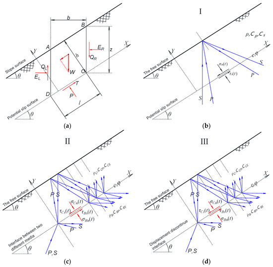
Figure 1.
The infinite slope model for instantaneous safety factor analysis: (a) static balance; (b) model I—continuous geo-material; (c) model II—interface between different geo-media; (d) model III—displacement discontinuous interface.
The first infinite slope model (model I) for instantaneous safety factor analysis is a continuous medium model (Figure 1b), the slope medium is continuous, and there is no waveform transformation and energy decomposition on the potential slip surface. The second model (model II) assumes that the slip surface is the interface between two mediums (Figure 1c), the upper medium with a thickness of h is the slip body (or cover layer), and the bottom medium is the basement layer. Moreover, the slip surface of third slope model (model III) is the displacement discontinuous interface in the slope model (Figure 1d). For these models, there are some assumptions:
(1) For model I, the potential slip surface is continuous, and the slope surface is the only boundary. Additionally, if there is no external load or constraint on the slope surface, it is treated as a free surface, and can be expressed as: , where , and are the stress components in the slope medium;
(2) For model II, the boundary conditions of slip surface for stress wave’s propagation satisfy: , , and , where are the stress components in the slope cover layer, and are the stress components in the slope basement layer; is the displacement in the slope cover layer, and is the displacement in the slope basement layer). Additionally, the slope surface is also treated as a free surface, which satisfies: ;
(3) For model III, the boundary conditions of slip surface for stress wave’s propagation satisfy: , , and , where , and are the normal and shear stiffness coefficients of slope slip surface. Moreover, the slope surface is also treated as a free surface, which satisfies: .
For the infinite slope model, the incident P-wave (the pressure wave) and SV-wave (the shear wave in model plane) are used in the slope model within any angle in the natural range . Before calculation, the instantaneous safety factor of slope, and the stress wave field in the cover layer and basement layer should be analyzed. In model I, the stress wave field is mixed with the incident wave (P- or SV-wave), reflected P-wave and SV-wave. However, in models II and III, the stress wave field is superposed with the upward P-wave, SV-wave, downward P-wave and SV-wave in the cover layer, and the wave field of basement layer is superposed with the incident wave (P- or SV-wave), downward P-wave and SV-wave. The symbols of stress wave’s amplitudes, propagation direction angle, and wave number of each stress wave in the medium are shown in Table 1.

Table 1.
Symbols of stress wave’s equations.
The wave field in the slope can be obtained by the elastic wave theory, and the boundary conditions of free surface and the continuous conditions of potential slip surface are used to obtain the solutions. The detailed solution processes are presented in Appendix A. When the amplitudes of stress wave are obtained, the stress components on slip surface can be calculated under the certain incident wave (by Equation (A15)), and the instantaneous safety factors can be written as:
where are the normal stress and shear stress along the slip surface (as shown in Figure 1).
3. Dynamic Response of Instantaneous Safety Factor
By Equation (2), the instantaneous safety factor Fs of infinite slope model can be obtained. As shown in Figure 2, when the P- or SV-wave is incident into the slope models with 30° angle (amplitude: 2.0 m/s2, frequency: 10.0 Hz), the safety factors of slope models I, II and III all fluctuate periodically over time, and the period equals to the period of incident wave (this can be recognized as the analytical solutions of Fs(t)). In addition, the differences of slip surface’s mechanical continuity, causing the instantaneous safety factor to fluctuate with different amplitudes and phases. As we know, in the stability analysis of seismic slope engineering, the extreme values of Fs are important variables to evaluate slope’s stability; therefore, the peak value , valley value and wave range will be discussed. Characteristic parameters of slope models and incident stress waves to slope stability will be calculated and compared in the follow sections.
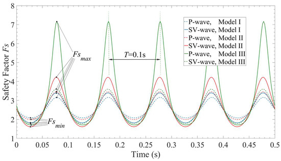
Figure 2.
Instantaneous safety factor Fs (the dynamic parameters of model I are , , ; , , , , , and are dynamic parameters for models II and III). (These values are roughly the mechanical parameters of hard sedimentary rocks in medium hardness.) The thickness of sliding body is , slope angle is , and slip surface’s mechanical strengths are Pa, and here. For model III, the normal stiffness and shear stiffness are Pa and Pa.
3.1. Effect of Slope Features
The slope angle, thickness of slip body, and mechanical parameters are the key variables that will affect the safety factor for a slope model. Based on the sensitivity analysis of the slope angle, the thickness of sliding body and the impedance ratio between the basement layer and cover layer, the influence of continuity of slip surface on the instantaneous safety factor is studied by the comparison method between models I, II and III. The model parameters of slope models are shown in Table 2; the slope angle changes in the range of 0–90° in case 1 (for soil slopes, there is a natural resting angle, but for rock slopes, the slope angle can be close to 90°), cover layer (or sliding body) thickness range (1.0–15.0 m) in case 2, and the wave impedance ratio (only for models II and III) between the basement layer and cover layer changes in the range of 1.0–49.0 in case 3. The ranges of cover layer’s thickness and the wave impedance ratio are determined by trial calculation, that is, the safety factor is basically stabilized with the change of these parameters.
Table 2.
The variables and parameters of slope features effect analysis (P- and SV-waves).
The safety factor of infinite slope will decrease with the slope angle, and the regularity also exists for the dynamic slope model; as shown in Figure 3, the peak value of dynamic slope safety factor decrease with slope angle nonlinearly, and the wave range decreases. Figure 3a is the comparison of instantaneous safety factor between models I and II; the slip surfaces change from the continuous state to the medium interface. Whether it is the incident P-wave or SV-wave, this change makes the peak safety factor higher and the valley safety factor lower. Figure 3b is the comparison of instantaneous safety factor between models II and III; the slip surfaces change from the interface of the medium to the displacement discontinuous interface. For this change, the variation of extreme instantaneous safety factor is different for the incident P-wave and SV-wave; when the P-wave is incident into the slope, the peak safety factor become higher and the valley safety factor becomes lower. However, when the SV-wave is incident into the slope, the peak safety factor becomes lower and the valley safety factor becomes higher.
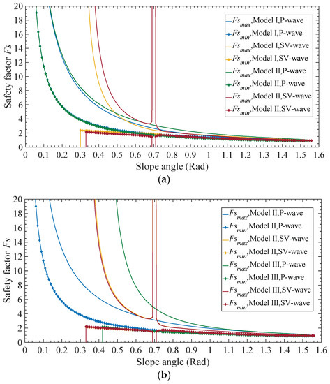
Figure 3.
Instantaneous safety factor vs. slope angle, and the incident direction keeps constant: (a) comparison between models I and II; (b) comparison between models II and III.
In Figure 3, there are some singular points existing for the extreme instantaneous safety factor curves, when the slope gets close to the horizontal direction and the critical angle for stress wave’s propagation. In Figure 3, when the slope angle is close to a certain value, the peak value trends to the positive infinity, and the valley value trends to the negative infinity. That is because the shear stress caused by gravity on the slip surface is close to the shear stress caused by the stress wave. The singular point also can be caused by the incident angle close to the critical angle of stress wave. With the increase of slope angle, the incident angle increases simultaneously; when the incident angle is close to the critical angle (here it is 40°), the singular points will occur by the non-uniform interface wave’s generation.
For the static problem, the safety factor of slope will decrease with slip body’s thickness monotonically, but it is becoming more complex for dynamic situations. As shown in Figure 4, for models I and II, the peak safety factor and the valley safety factor all decrease with thickness monotonically, but for model III, as shown in Figure 4b, the peak value will appear in the manner of decrease–increase–decrease with the incident SV-wave, and in a certain range, the critical points exist; and when thickness of sliding body is close to critical points, the peak value increases rapidly, and the valley value becomes negative. By the comparison between models I, II and III, it can be found that if the slip surface changes from the continuous state to the interface of the medium, whether it is the incident P-wave or SV-wave, this change makes the peak safety factor higher and the valley safety factor lower. Moreover, if the slip surface changes from the interface of the medium to the displacement discontinuous interface, the variation of extreme instantaneous safety factor is different for the P-wave and SV-wave; with the incident P-wave, the peak safety factor becomes higher and the valley safety factor becomes lower; however, when the SV-wave is incident into the slope, the peak safety factor becomes lower and the valley safety factor becomes higher.
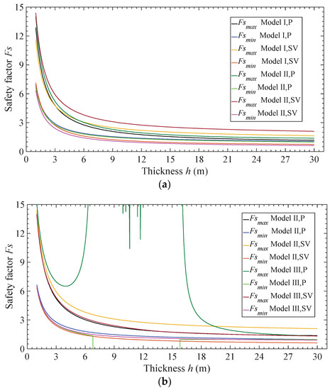
Figure 4.
Instantaneous safety factor vs. thickness of slip body: (a) comparison between models I and II; (b) comparison between models II and III.
For the slope models II and III, wave impedance of material is an important factor for slope’s instantaneous safety factor. In most situations, the wave impedance of basement layer is larger than cover layer’s wave impedance; therefore, the wave impedance ratio is considered as the variable to analyze the dynamic response of safety factors. From Figure 5, it can be found that peak safety factor increases with the wave impedance ratio , and the valley safety factor decreases with the wave impedance ratio . When the slip surface changes from the interface of the medium to the displacement discontinuous interface, the peak safety factor becomes higher for the incident P-wave and the valley safety factor becomes lower for the incident SV-wave.
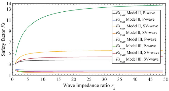
Figure 5.
Instantaneous safety factor vs. wave impedance ratio .
3.2. Effect of Incident Stress Wave
In order to analyze the influence of incident wave on the instantaneous safety factor, the amplitudes, frequency and incident angle will be taken as the investigated variables in the following discussion. The model parameters of slope models are shown in Table 3, the incident wave’s amplitude changes in the range of 0.1–6.0 m/s2 in the case 4, the wave’s frequency range is 5–200 Hz in case 5, and the incident angle (P- and SV-waves) changes in the range of 1.0–90.0° in case 6. (The ranges of wave’s amplitudes and frequency ensure that Figure 6, Figure 7 and Figure 8 can show the change of instantaneous safety factor more completely.)
Table 3.
The variables and parameters for stress wave’s effect analysis (P- and SV-waves).
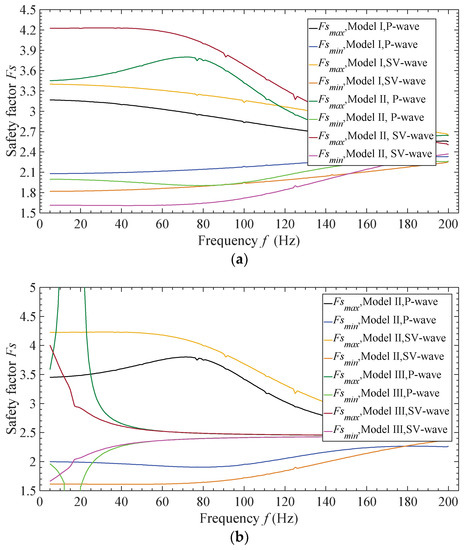
Figure 6.
Instantaneous safety factor vs. wave frequency: (a) comparison between models I and II; (b) comparison between models II and III.
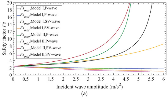
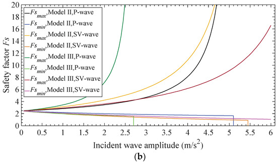
Figure 7.
Instantaneous safety factor vs. wave’s amplitude: (a) comparison between models I and II; (b) comparison between models II and III.
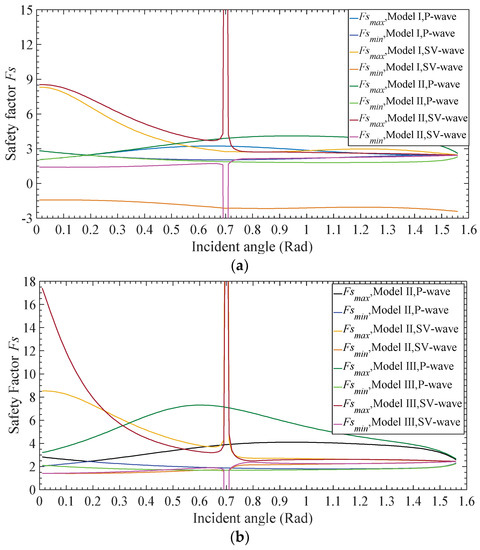
Figure 8.
Instantaneous safety factor vs. wave incident angle: (a) comparison between models I and II; (b) comparison between models II and III.
The influence of the frequency of incident wave on the instantaneous safety factor is nonlinear. Based on the comparison of models I and II, as shown in Figure 6a, when the slip surface changes from the continuous surface to interface of medium, the peak safety factor becomes higher and the valley safety factor becomes lower, and the trend changes from monotonous to a more complex form—first increase and then decrease. When the slip surface changes from interface of medium to displacement discontinuous surface, as shown in Figure 6b, the trend of extreme value of instantaneous safety factor becomes more complex, and a singular point exists. The peak value increases when the frequency is close to the singular point, and the valley value decreases when the frequency is close to the singular point.
With the increase of incident wave’s amplitude, more wave energy will transmit into the slope body, the fluctuation range of instantaneous safety factor becomes larger, the valley value becomes lower, and the peak value becomes higher. As shown in Figure 7, the effect of slip surface’s continuity properties is similar to the above analysis. In addition, as the stress wave’s amplitude increases, the valley value of instantaneous safety factor will be negative value, and this phenomenon caused by the dynamic shear stress is larger than the static shear stress on the slip surface.
The effect of incident angle on the instantaneous safety factor is complicated; under superposition of reflected wave on the slope surface, and the reflected and the transmitted waves on the slip surface, the extreme value of instantaneous safety factors changes with the incident angle nonlinearly. As shown in Figure 8, when the slip surface changes from the continuous interface to the interface of medium, the peak value becomes higher for the incident P-wave, and the valley value becomes lower. When the slip surface changes from the interface of medium to the displacement discontinuous interface, the peak value becomes higher for the incident P-wave, and the valley value becomes lower for the incident P-wave and higher for the incident SV-wave. In particular, for the same changes, with the incident SV-wave, the peak value becomes higher in the range of smaller incident angles, and becomes lower in the larger incident angle range (Figure 8). For the slope models II and III, the critical angle exits with the incident SV-wave, and the singular point will occur.
3.3. Effect of Deformation Stiffness of Slip Surface
For displacement discontinuous slip surface, the deformation stiffness will influence stress wave’s propagation significantly. The model parameters of slope models are shown in Table 4, and the stiffness coefficient is used as a variable to analyze the effects of slip surface’s continuity (in case 7). According to previous studies, when the displacement discontinuous surface deformation stiffness coefficient increases to infinity, the discontinuous interface will become the interface of medium. Thus, the deformation stiffness analysis of model III will be compared with models I and II separately.
Table 4.
The variables and parameters for effect analysis of deformation stiffness of discontinuous surface (P-, and SV-waves).
Because the deformation stiffness coefficient of sliding surface controls the transmission of stress wave energy, the fluctuation range of safety factor is equal to zero when the stiffness coefficients . As shown in Figure 9, the instantaneous safety factor does not monotonically increase or decrease as the stiffness coefficient increases. Based on the comparison of slope models I and III (Figure 9a), the slip surface’s deformation stiffness makes the continue interface become the displacement discontinuous interface, and the instantaneous safety factor of model III will be close to the value of model I when the deformation stiffness coefficient trends to infinity. From the continuous slip surface to the displacement discontinuous surface, the peak value increases and the valley value decreases with the incident P-wave, and the peak value decreases and the valley value increases with the incident SV wave. This variation is established when the deformation stiffness value is greater than a certain value; when the deformation stiffness value is less than a certain smaller value, the variation becomes opposite. These regularities also apply to the change from the medium interface to displacement discontinuous surface, as shown in Figure 9b.
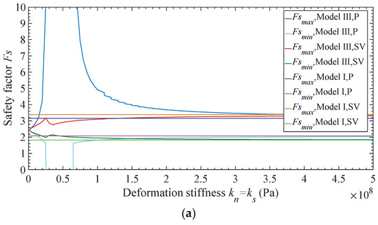
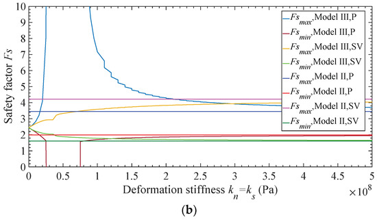
Figure 9.
Instantaneous safety factor vs. deformation stiffness : (a) comparison between models I and II; (b) comparison between models II and III.
4. Discussion
Based on the above analysis, the effect of the continuity of slip surface on the slope safety factor was studied preliminarily. In engineering, the discontinuous surface is widely found in rock and soil, usually manifested in the form of surface of stratum, fracture, joints or faults. For dynamic geotechnical problems, discontinuous surfaces not only affect the mechanical properties of rock mass, but also significantly affect the propagation of stress waves. Therefore, a large number of literatures have carried out the in-depth analysis of the stress wave propagation behavior of non-continuous surface of rock and soil. In the earlier research, the medium interface is used to describe the phenomenon of stress wave propagation [3,4], but with the further study of rock mechanics, it is found that the mechanical deformation of rock mass structure is very complex, showing strong nonlinear properties. The displacement discontinuous model is generally used to describe the propagation of stress waves [7,8,9,10,11,12,13,14,15,16]. Because these two typical discontinuous surface models can describe the stress wave propagation behavior of most discontinuous surface in rock or soil, it is used to describe the stress wave behavior of sliding surface in slope.
According to properties of slip surface, the slope models were divided into three types. From model I to model III, as shown in Figure 10, the continuity of the slip surface gradually decreases, and the transmittance of stress wave energy is also gradually decreasing. However, the safety factor of the slope does not increase or decrease monotonously with the decrease of slip surface’s continuity. Through the analysis in the previous section, it is found that when the slip surface changes from the continuous surface to the medium interface, the peak value of the instantaneous safety factor becomes higher when the P-wave or SV-wave are incident on the surface, and the valley value becomes lower. Further, if the slip surface changes from the medium interface to the displacement discontinuous surface, the change of safety factor depends on the type of incident wave. With the incident P-wave, the peak value of the instantaneous safety factor becomes higher, and the valley value becomes lower; however, with the incident SV-wave, the of the instantaneous safety factor becomes higher, and the becomes lower. These changing rules can be applied in most cases, it becomes different when the incident angle of stress wave becomes smaller, or when the deformation stiffness coefficient of slip surface becomes smaller (as shown in Figure 8 and Figure 9). Therefore, it can be seen that the effect of slip surface’s continuity on slope stability is complex and variable. Specifically, the wave field superimposed by the reflected, refracted and interference waves, so that the stress components on the slide surface are related to the incident wave type, incident angle, slope dimension and mechanical properties. The method in this paper is an accurate and effective method to analyze the influence of the continuity of sliding surface on the dynamic response of infinite slope.
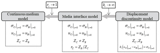
Figure 10.
Continuity changes of models I, II and III (i = x, y).
The infinite slope model is used as the basic model to solve the solution, so that it has the better boundary condition to consider the reflection of slope surface as a free surface. For the general slope, the irregular shape of slope surface cannot help obtain the theoretical solution, which makes the numerical simulation and the physical model experiment become very necessary [18,19,20,21]. In some literatures, the reflection of the slope surface is not considered [20,21], and the assumption that the slope surface can absorb stress wave is made The influences of slope surface’s reflection are analyzed in Figure 11 and Figure 12.
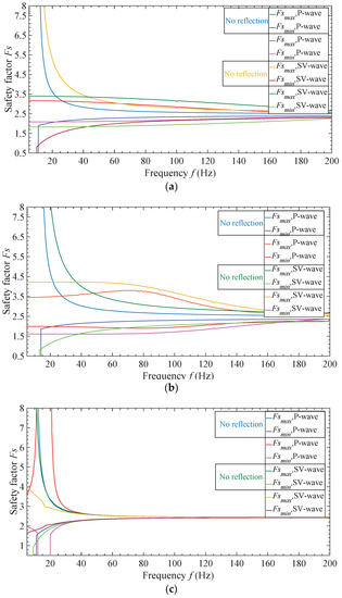
Figure 11.
Comparison of free slope surface with reflection and no reflection (instantaneous safety factor vs. wave frequency): (a) model I; (b) model II; (c) model III.
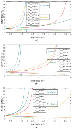
Figure 12.
Comparison of free slope surface with reflection and no reflection (instantaneous safety factor vs. wave amplitude): (a) model I; (b) model II; (c) model III.
As shown in Figure 11, without the interference of slope surface, the changing curves of slope instantaneous safety factor become monotonous, the peak value decreases with frequency and the valley value increases with the frequency monotonically. Within a lower frequency range, the valley value in the case of non-reflection surface is lower than that in the case of reflection surface. However, within a higher frequency range, the valley value of safety factor in the case of non-reflection surface is larger than that in the case of reflection surface. Therefore, the influence of incident wave frequency on slope safety should be analyzed in different ways, according to the slope surface’s reflection or non-reflection.
As shown in Figure 12, without the interference of slope surface, the changing curves of slope instantaneous safety factor are similar to those in the case of considering the reflection of slope surface. With the increasing of wave’s amplitude, the peak value of safety factor increases, and valley value decreases. Moreover, the changing rate of safety factor in the case of non-reflection surface is larger than that in the case of reflection surface.
By this investigation, we found that the continuity of slip surfaces in the engineering site is an important factor for seismic slope stability, which should be analyzed carefully. Continuity of slip surface, the features of slope and characteristics of incident waves can control the slope safety factor in different ways. Additionally, for the infinite slope, the methods proposed in this paper can analyze the influence of continuity of slip surface on stability. Based on the method and model in this research, the instantaneous safety factor can be obtained by theoretical methods with the incident simple harmonic P-wave and SV-wave. Furthermore, this method can be used to acquire the instantaneous safety factor of infinite slope under any earthquake action, the seismic wave can be decomposed into series of harmonic waves by the time–frequency analysis method (like HHT based methods presented in literature [20]), and the instantaneous safety factor can be obtained by the superposition of stress components on the slip surface.
5. Conclusions
In this paper, the influences of the stress wave propagation properties of the slip surface on slope stability are analyzed and discussed. The main findings can be summarized as follows:
- The instantaneous safety factor of the slope does not simply increase or decrease with the decrease of the continuity of the slip surface, but significantly changes with the frequency of the incident wave, the incident angle and the deformation stiffness of the slip surface. However, in most cases, some significant regularities can be found:
- (a)
- When slip surface changes from the continuous surface to medium interface, it leads to the higher peak value of instantaneous safety factor, and the lower valley value;
- (b)
- When slip surface changes from the medium interface to displacement discontinuous surface, it leads to the higher peak value, and the lower valley value with the incident P-wave, and leads to the lower peak value lower, and the higher valley value with the incident SV-wave.
- Without the reflection of slope surface, the changing trend of peak value and valley value of instantaneous safety factor will become much simpler. Compared with instantaneous safety factor considering the reflection of slope surface, at lower frequencies, the peak value becomes higher and the valley value becomes lower; but at higher frequencies, the peak value becomes lower and the valley value becomes higher.
- Different from the static problem, as the slope angle and thickness of slip body increase, the instantaneous safety factor will not monotonically decrease.
- With the lower frequency and higher amplitude of incident wave, the valley value of instantaneous safety factor will be lower, and more unstable for the slope. Additionally, this kind of situation should be noticed in the engineering.
Based on this study, the continuity of structure surface should be investigated prior to the slope stability analysis, which will affect the dynamic response of slope in different ways for different types of structure surface.
Author Contributions
All the authors contributed to publishing this paper, C.L. contributed to the formulation of the overarching search goals and aims; G.W. and W.H. contributed to the theoretical formula derivation and content optimization.
Funding
This research was funded by the Natural Science Foundation of Southwest University of Science and Technology, Multi-dimensional time–frequency analysis of the seismic response of bedding rock slopes, No.17zx714.
Conflicts of Interest
The authors declare no conflict of interest.
Appendix A
In the infinite slope model, the wave equations in the cover layer (the sliding body) can be written as:
where the equation is the wave equations of P-wave containing upward and downward P-waves; and is the wave equation of SV-wave containing the upward and downward SV-waves. The wave numbers are , and . Additionally, the wave equations in the basement layer are:
where the equation is the wave equation of P-wave in the basement layer containing incident and reflected P-waves, and is the SV-wave equation containing the incident and reflected SV-waves. The wave numbers are , and . The displacement can be obtained by:
where ; . Then, the strain–displacement relationship and Hoek’s law can obtain the strain components and stress components. For the stress wave’s field solutions, the boundary conditions of slope surface and the slip surface are used to solve the unknown amplitudes of stress wave in the cover layer and the reflection waves in the basement layer.
For model II, the boundary conditions are:
For model III, the boundary conditions are:
Then, the equations for solving unknown amplitudes can be written as:
where ; M, and are the coefficients which are the functions of slope configuration, dynamic parameters of geo-material, stress wave’s parameters, and related to the type of model. For model II:
For model III:
After the amplitudes of stress waves are obtained, the stress on the slip surface can be calculated as:
References
- Wu, X.; Jiang, Y.; Guan, Z.; Wang, G. Estimating the support effect of the energy-absorbing rock bolt based on the mechanical work transfer ability. Int. J. Rock Mech. Min. Sci. 2018, 103, 168–178. [Google Scholar] [CrossRef]
- Li, X. Rock Dynamic Fundamentals and Applications; Science Press: Beijing, China, 2014. [Google Scholar]
- Knott, C.G. Reflexion and refraction of elastic waves, with seismological applications. Philos. Mag. 1924, 48, 64–97. [Google Scholar] [CrossRef]
- Zoeppritz, K. Erdbebenwellen VIII B, Uber Reflexion and Durchgang seismischer wellen durch Unstetigkeisflachen. Gott. Nachr 1919, 1, 66–84. [Google Scholar]
- Mindlin, R.D. Waves and vibrations in isotropic, elastic plates. In Structural Mechanics; Goodier, J.N., Hoff, N.J., Eds.; Pergamon Press: New York, NY, USA, 1960; pp. 199–232. [Google Scholar]
- Kendall, K.; Tabor, D. An Ultrasonic Study of the Area of Contact between Stationary and Sliding Surfaces. Proc. R. Soc. Lond. Part A 1971, 323, 321–340. [Google Scholar] [CrossRef]
- Schoenberg, M. Elastic wave behavior across linear slip interfaces. J. Acoust. Soc. Am. 1998, 68, 1516–1521. [Google Scholar] [CrossRef]
- Gu, B.; Suárez-Rivera, R.; Nihei, K.T.; Myer, L.R. Incidence of plane waves upon a fracture. J. Geophys. Res. Solid Earth 1996, 101, 25337–25346. [Google Scholar] [CrossRef]
- Liu, C.; Zhang, J.; Cui, P. Reflection and refraction laws of low amplitude stress wave on a 3D rock joint surface. J. Vib. Shock 2018, 37, 68–77. [Google Scholar]
- Pyrak-Nolte, L.J.; Myer, L.R.; Cook, N.G.W. Transmission of seismic waves across single natural fractures. J. Geophys. Res. 1990, 95, 8617–8638. [Google Scholar] [CrossRef]
- Pyrak-Nolte, L.J. The seismic response of fractures and the interrelations among fracture properties. Int. J. Rock Mech. Min. Sci. Geomech. Abstr. 1996, 33, 787–802. [Google Scholar] [CrossRef]
- Suarez-Rivera, F.R.; Cook, N.G.W.; Myer, L.R. Study on the transmission of shear waves across thin liquid films and thin clay layers. In Proceedings of the 33th U.S. Symposium on Rock Mechanics (USRMS), Santa Fe, NM, USA, 3–5 June 1992. [Google Scholar]
- Daehnke, A.; Rossmanith, H.P. Reflection and refraction of plane stress waves at interfaces modelling various rock joints. Fragblast 1997, 1, 111–231. [Google Scholar] [CrossRef]
- Funahashi, F.; Yoshioka, N. Effects of Contact Geometry of Faults on Transmission Waves. Pure Appl. Geophys. 2001, 158, 717–739. [Google Scholar] [CrossRef]
- Zhao, J.; Cai, J.G. Transmission of Elastic P-waves across Single Fractures with a Nonlinear Normal Deformational Behavior. Rock Mech. Rock Eng. 2001, 34, 3–22. [Google Scholar] [CrossRef]
- Yu, J.; Song, X.; Qian, Q. Propagation of p-waves in dual nonlinear elastic medium for jointed rock mass. Chin. J. Rock Mech. Eng. 2011, 30, 2463–2473. [Google Scholar]
- Zheng, Y.; Hailin, Y.E.; Huang, R.; Li, H.; Xu, J. Study on the seismic stability analysis of a slope. J. Earthq. Eng. Eng. Vib. 2010, 30, 173–180. [Google Scholar]
- Ni, W.; Tang, H.; Liu, X.; Wu, Y. Dynamic stability analysis of rock slope considering vibration deterioration of structural planes under seismic loading. Chin. J. Rock Mech. Eng. 2013, 32, 492–500. [Google Scholar]
- Liu, X.; Liu, Y.; He, C.; Li, X. Dynamic stability analysis of the bedding rock slope considering the vibration deterioration effect of the structural plane. Bull. Eng. Geol. Environ. 2016, 77, 1–17. [Google Scholar] [CrossRef]
- Yang, C.; Zhang, J.; Bi, J. Application of Hilbert-Huang Transform to the analysis of the landslides triggered by the Wenchuan earthquake. J. Mt. Sci. 2015, 12, 711–720. [Google Scholar] [CrossRef]
- Fan, G.; Zhang, L.; Zhang, J.; Yang, C. Time-frequency analysis of instantaneous seismic safety of bedding rock slopes. Soil Dyn. Earthq. Eng. 2017, 94, 92–101. [Google Scholar] [CrossRef]
- Ali, A.; Huang, J.; Lyamin, A.V.; Sloan, S.W.; Griffiths, D.V.; Cassidy, M.J.; Li, J. Simplified quantitative risk assessment of rainfall-induced landslides modelled by infinite slopes. Eng. Geol. 2014, 179, 102–116. [Google Scholar] [CrossRef]
- Prisco, C.D.; Pastor, M.; Pisanò, F. Shear wave propagation along infinite slopes: A theoretically based numerical study. Int. J. Numer. Anal. Methods Geomech. 2012, 36, 619–642. [Google Scholar] [CrossRef]
- Conte, E.; Troncone, A. A performance-based method for the design of drainage trenches used to stabilize slopes. Eng. Geol. 2018, 239, 158–166. [Google Scholar] [CrossRef]
© 2019 by the authors. Licensee MDPI, Basel, Switzerland. This article is an open access article distributed under the terms and conditions of the Creative Commons Attribution (CC BY) license (http://creativecommons.org/licenses/by/4.0/).