Article

Imperfect Multi-Stage Lean Manufacturing System with Rework under Fuzzy Demand

by
Muhammad Tayyab
1,
Biswajit Sarkar
1,* and
Bernardo Nugroho Yahya
2
1
Department of Industrial & Management Engineering, Hanyang University, Ansan Gyeonggi-do 155 88, Korea
2
Industrial and Management Engineering Department, Hankuk University of Foreign Studies, 81, Oedae-ro, Mohyeon-myeon, Cheoin-gu, Yongin-si, Gyeonggi-do 17035, Korea
*
Author to whom correspondence should be addressed.
Mathematics 2019, 7(1), 13; https://doi.org/10.3390/math7010013
Submission received: 19 November 2018 / Revised: 19 December 2018 / Accepted: 19 December 2018 / Published: 24 December 2018

Abstract

:
Market conditions fluctuate abruptly in today’s competitive environment and leads to imprecise demand information. In particular, market demand data for freshly launched products is highly uncertain. Further, most of the products are generally manufactured through complex multi-stage production systems that may produce defective items once they enter the out-of-control state. Production management of a multi-stage production system in these circumstances requires robust production model to reduce system costs. In this context, this paper introduces an imperfect multi-stage production model with the consideration of defective proportion in the production process and uncertain product demand. Fuzzy theory is applied to handle the uncertainty in demand information and the center of gravity approach is utilized to defuzzify the objective function. This defuzzified cost objective is solved through the analytical optimization technique and closed form solution of optimal lot size and minimum cost function are obtained. Model analysis verifies that it has successfully achieved global optimal results. Numerical experiment comprising of three examples is conducted and optimal results are analyzed through sensitivity analysis. Results demonstrate that larger lot sizes are profitable as the system moves towards a higher number of stages. Sensitivity analysis indicates that the processing cost is the most influencing factor on the system cost function.

1. Introduction

Lean manufacturing concepts are becoming rapidly popular in global production industries subjected to growing market competitions and increased manufacturing costs. Initiated by Toyota’s engineer Taiichi Ohno, credited with developing the principles of lean production after World War II; eliminating unwanted activities, empowering workforce, cut down inventories, and improving productivity are the focused themes of lean philosophy. Unlike Henry Ford, who maintained resources in expectation of what might be required for future manufacturing, the management team at Toyota built partnership with suppliers and consequently became made-to-order. Thus, they can easily handle quick changes, and opposite to what their competitors could, they became able to respond quicker to market demands.
Highly inflexible and having high volume/low variety products of automatic machinery are the constraints in the textile industries. Due to this nature of textile industry, implementation of lean manufacturing is a challenge in this industry. Therefore, value stream mapping, kaizen, 5S, kanban, poka-yoke, and visual controls are practiced in combination with each other to improve the textile manufacturing process [1]. Most of the textile manufacturing processes include more than one production stages, and among all other concerns, optimum work in process inventory levels and scrap control are the premier ones. Thus, managers are interested in working out ways to minimize total system costs through optimal lot sizing in the production system. This builds importance of economic production quantity model in this sector to escape high inventory levels and cut down production costs. Figure 1 shows a general multi-stage production flow of an apparel manufacturing industry.
Since Harris [2] and Taft [3] provided Economic Order Quantity (EOQ) and Economic Production Quantity (EPQ) formulas, respectively, economic lot size models are broadly developed by the researchers. Due to their simplicity, these inventory models are used in many applied situations. In the inventory management research, Lee [4], Gupta and Chakraborty [5], and Tayi and Ballou [6] studied reprocessing of imperfect items, in which shortages due to reworking were not taken into account by the last two. Lee et al. [7] and Glock and Jaber [8] provided production models for imperfect production systems without considering rework opportunity. C.S Lin [9] studied the production process for its out-of-control state along with raw material resource constraints. Salameh and Jaber [10] provided an inventory model for imperfect quality items where these items are withdrawn from stock resulting in lower holding cost per unit time. Their model was extended by Khan et al. [11], and Jaber et al. [12] considers strategies for handling these imperfect quality items. Ouyang et al. [13] and Cárdenas-Barrón [14] formulated inventory models in which backordering is allowed and Eroglu and Ozdemir [15] considered shortages in their studies. Jaber and Guiffrida [16] studied Wright’s learning curve along with preventive maintenance, and Daya [17] likewise extended the inventory model with planned maintenance schedules.
Most of the researchers developed inventory models for single-stage imperfect production systems, where numerous of them focused on analysis of the defective rates. Reworking in single-stage inventory models with constant defective rates has been established by Jamal et al. [18], Biswas and Sarker [19], Chung [20], and Taleizadeh et al. [21], in which the latter two included backordering in their models. Cárdenas-Barrón [22] extended the inventory model provided by Jamal et al. [18] with the addition of the algebraic solution approach. Ma et al. [23] analyzed imperfect production system without providing reworking alternatives in their model, and Barzoki et al. [24] presented discounted sales of non-reworkable items. Other researchers modified inventory model with random-defective rate in single-stage manufacturing system, where the reworking option was assumed by Chiu et al. [25], Chiu et al. [26], Noorollahi et al. [27], Haider et al. [28], and Chiu et al. [29] using the renewal reward theorem. Taleizadeh et al. [30] allowed a backordering alternative along with the rework prospect in their inventory model, whereas Chiu et al. [31] and Taleizadeh et al. [32] developed inventory models, ignoring the reworking facility. Random defect-rate contemplation was further established by Sana [33], Sarkar and Moon [34], Yoo et al. [35], Chakraborty and Giri [36], Wee et al. [37], Chiu et al. [38], and Sarkar et al. [39] using a number of other shop-floor conditions.
In real situations, determining the precise value of product demand is very difficult. To deal with such conditions, managers need to gather demand data from the experts. If, according to the experts, demand about some randomly chosen quantity is fixed; their opinion is imprecise and then the expected annual demand is vaguely expressed. This explanation of demand is through a fuzzy number. As defined by Dang and Hong [40], fuzziness is some parametric property of the demand captured when its sharp boundaries cannot be determined by the decision makers. Zadeh [41] introduced fuzzy terminologies in 1978. After him, several researches including Petrovic and Sweeney [42], Roy and Maiti [43], Yao and Su [44], Chang and Ouyang [45], Mahata and Goswami [46], and De and Goswami [47] formulated inventory models considering parameters like demand, total average cost, storage space, and holding cost as fuzzy numbers. Numerous other researches solved inventory models considering fuzzy demand. Chang and Yeh [48], Sadeghu and Niaki [49], Lin et al. [50], Cosgun et al. [51], and Sadeghi et al. [52] treated demand as a trapezoidal fuzzy number in their inventory models. Some other researchers including Rong and Maiti [53], Zhang et al. [54], Moghaddam [55], and Huang et al. [56] considered demand as a Triangular Fuzzy Number (TFN). In addition, Taleizadeh et al. [57] presented a multi-constraint EOQ model with incremental discounts and uncertain item cost under fuzzy environment, and Jana et al. [58] considered storage space and available budget as fuzzy variables. Das et al. [59] assumed credit period in a supply chain as a fuzzy number, and Kumar and Goswami [60] developed a production inventory model under fuzzy shifting time to out-of-control state and fuzzy defective proportion.
In fact, in real situations, production processes are imperfect, thus producing defective items at a certain rate. That is why many researchers and practitioners have formulated inventory models expressing different real world circumstances [21,22,23,24]. In addition, parametric information of the real world production systems is not always known with precision [48]. This imprecise data can be random or uncertain in nature. Probability theory can handle the situations with random information, whereas the computational methods provided by the fuzzy theory are required to tackle the uncertain conditions. Several approaches including the signed distance method, min-max approximation, weighted average method, the center of gravity approach (centroid method), and center of the largest area are available in the uncertainty control literature to model the uncertain environment. This research work has used the center of gravity approach to grasp the uncertainty in demand information because of its simplicity and ease of use.
Vast research has been done on single-stage production system, in which machine breakdowns and defective proportion are considered as constant, random, and occasionally fuzzy in nature [22,34,60]. Regarding multistage production systems, only a few economic batch quantity models are available with limited real world production scenarios to provide succor in decision making for the managers dealing with multi-stage production systems [61,62]. This paper attempts to add in the literature by formulating an economic lot size model for multi-stage production facility with setup time requirement, uncertain annual demand rate, and imperfection constraints. The aim of this research work is to initiate a multi-stage production model by considering a real world shop-floor situation of defective production and uncertain market conditions regarding demand information.
Literature analysis indicates that no such model exists in the current research stream of the inventory and production management. This fact provides motivation for the development of multi-stage production model with the aforementioned attributes. Thus, the novelty of this study is the introduction of imperfect production proportion at each stage of the multi-stage production system and imprecise product demand. The objective of the research is to minimize the total cost of the imperfect multi-stage production system by determining optimal lot size under uncertain environments. Fuzzy theory is applied to grasp the uncertainty in demand information and analytical optimization technique is applied to obtain global optimum results of the model. The model is analyzed through sensitivity analysis and significant conclusions are obtained that verifies the substantial contribution of the proposed model in the inventory research literature.
Framework of the paper is as follows: The mathematical model is developed in Section 2. Section 3 provides experimental study and optimal results. Section 4 presents discussion and analysis of the proposed production model. Finally, in Section 5, concluding remarks and future research directions of this paper are discussed.

2. Materials and Methods

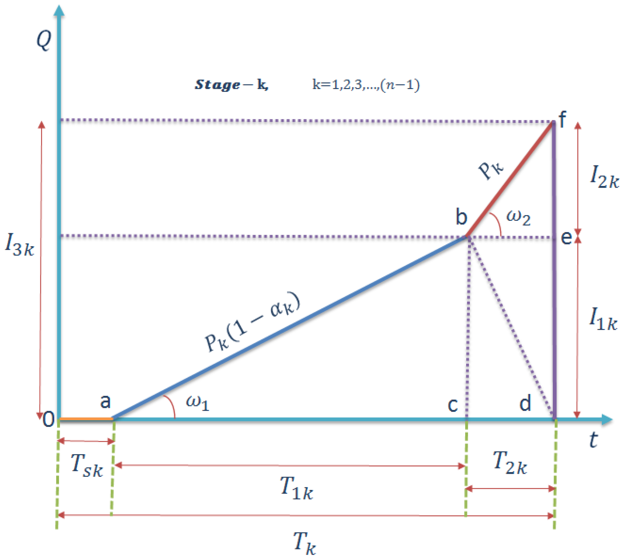
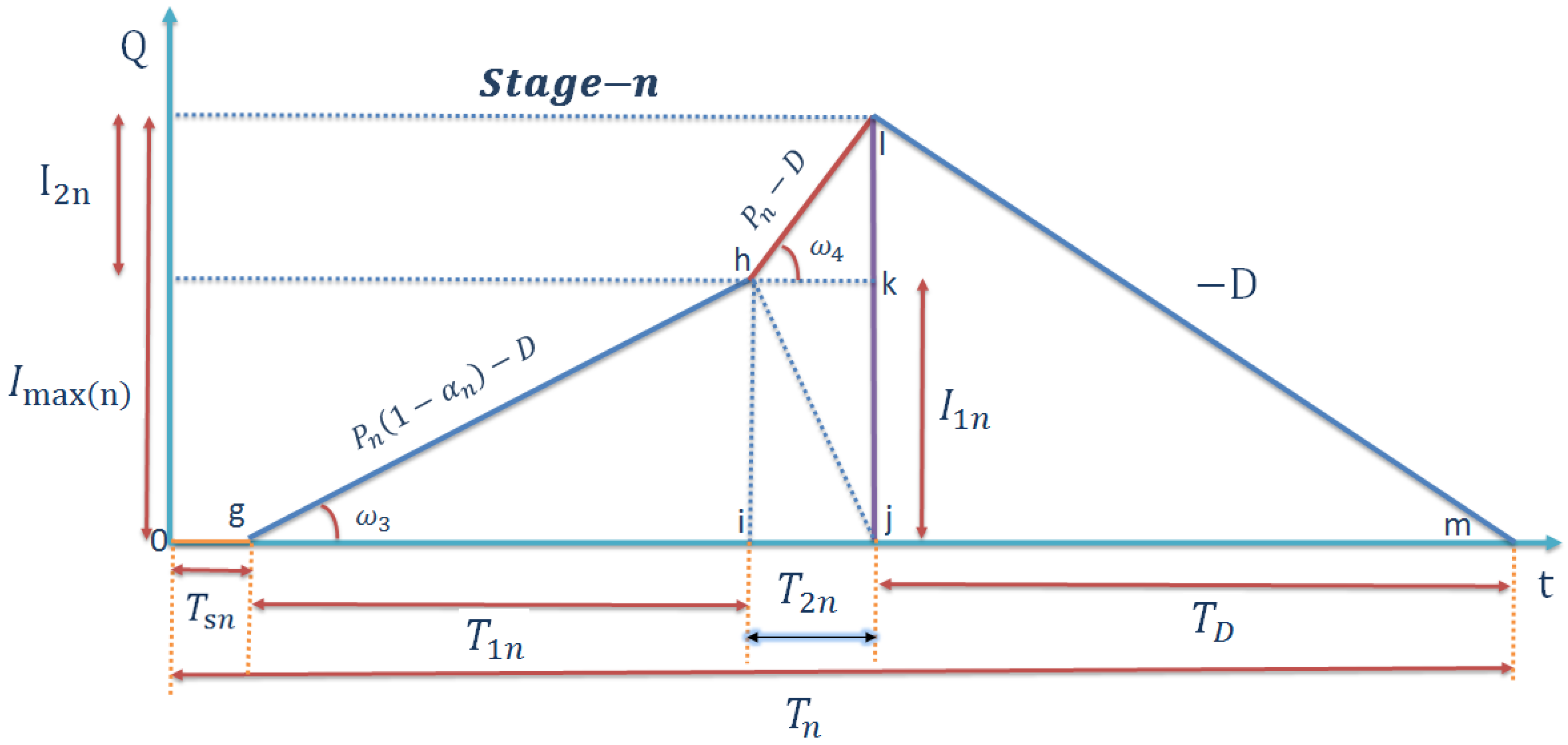
This research work studies an n -stage imperfect production system where defective items are produced along with the perfect quality items. These defective items are reworked at an additional processing cost, and product demand is fulfilled at the n t h production stage. Figure 2 and Figure 3 show inventory behavior of production stage-k and production stage-n, respectively. The objective of the model is to minimize the total system cost by determining optimal lot size.

2.1. Assumptions

Following assumptions are considered in the development of multi-stage production model.
  • A single type of item is produced in an n-stage production system.
  • Production runs are fairly consistent, i.e., system is assumed to be a lean manufacturing system where inventory behavior follows a similar trend in repetitive production cycles.
  • Uncertain product demand is measured as a Triangular Fuzzy Number (TFN).
  • Inline inspections provides effective results, determines the defective items immediately, and helps the managers to make immediate decisions over it. This model assumes that defective items are detected during the hundred percent inline inspection.
  • In textile industries, defective items are generally reworked. This model assumes reworking of defective items at each production stage. The reworking process is considered as perfect and no item is scrapped.
  • Defective rate is constant at each production stage, but it may vary from stage to stage.
  • Setup time of each production stage is ρ percent of the total time of that production stage.
  • Transportation time and cost among the production stages is assumed to be negligible.

2.2. Model Formulation

Keeping in view the above-mentioned assumptions, a mathematical model is formulated.
Figure 2 shows the inventory behavior of k t h production stage. Maximum inventory level ( I 3 k ) of the k t h production stage ( k = 1 , 2 , 3 , , n 1 ) is computed as I 3 k = I 1 k + I 2 k , where I 1 k is the inventory level after production phase and I 2 k is the inventory level after reworking phase.
Production time of stage-k is T 1 k = Q P k , and its reworking time is T 2 k = Q α k P k . It is obvious from triangle abc in Figure 2, that tan ω 1 = I 1 k T 1 k , which gives I 1 k = Q ( 1 α k ) . Similarly, from triangle bef, one can observe that tan ω 2 = I 2 k T 2 k , which provides I 2 k = Q α k . From above the maximum inventory level of k t h production stage is obtained as I 3 k = Q .
Total inventory of k t h production stage is the sum of the triangular areas abc, bcd, and bdf (Figure 2). One can simply compute these areas and the total inventory of k t h production stage is now formulated as:
I k = Q 2 2 P k ( 1 + α k α k 2 )
Total production time of stage- k can be obtained by the sum T k = T s k + T 1 k + T 2 k , where the setup time of stage- k , T s k = ρ ( T 1 k + T 2 k ) . Total time of stage- k ( T k ) is obtained as:
T k = Q P k ( 1 + ρ ) ( 1 + α k )
Applying similar method for production stage- n (Figure 3), one can simply obtain production time T 1 n = Q P n , reworking time T 2 n = Q α n P n , pure consumption time T D = Q D ( 1 D P n ( 1 + α n ) ) , inventory level after production phase I 1 n = Q ( 1 α n D P n ) , and inventory level after reworking phase as I 2 n = Q α n ( 1 D P n ) for production stage-n. Finally, maximum inventory level of stage-n is computed as I max ( n ) =   Q ( 1 D P n ( 1 + α n ) ) .
Proceeding towards determination of total inventory level of finished items ( I ), we have
I = Q 2 2 D ( 1 D P n ( 1 + α n + α n 2 ) )
Total time of production stage- n is obtained as
T n = ( 1 + ρ ) Q D
Total time of the complete production system can be determined by the sum T = k = 1 n 1 T k + T n , and is given by
T = Q ( 1 + ρ ) D ( 1 + D k = 1 n 1 ( 1 + α k P k ) )
Average inventory level of the finished items ( I ¯ ) in the system is calculated as I ¯ = I T , which provides
I ¯ = Q ( P n D ( 1 + α n + α n 2 ) ) 2 P n ( 1 + ρ ) ( 1 + D k = 1 n 1 ( 1 + α k P k ) )
Total cost of the system by considering setup cost, order processing cost, inspection cost, and inventory holding cost is formulated as follows:
Setup cost ( K S ) ($K/lot/stage)
Setup cost is a major part of the total cost in a production system. It is required to be incurred prior to the production of every lot. For an n-stage production system, the total setup cost is
K s = i = 1 n K i
Order processing cost ( K P ) ($C/item/stage)
Order processing cost and reworking cost are considered as the same in this model. The total order processing cost is the sum of processing cost of good items as well as the reworking cost of defective items:
K P = Q i = 1 n C i ( 1 + α i )
Inspection cost ( K I ) ($J/item/stage)
Inspection cost is incurred on both good quality items as well as on reworked items and is assumed to be the same. Total inspection cost:
K I = Q i = 1 n J i ( 1 + α i )
Inventory holding cost ( K C ) ($H/item/year)
Under linear assumptions, total inventory holding cost is proportional to the holding cost of average inventory of finished items in the cycle as
K C = H I ¯ = H Q ( P n D ( 1 + α n + α n 2 ) ) 2 P n ( 1 + ρ ) ( 1 + D k = 1 n 1 ( 1 + α k P k ) )
Total system cost function by considering aforementioned cost components is given by
T C ( Q ) = i = 1 n K i + Q i = 1 n C i ( 1 + α i ) + Q i = 1 n J i ( 1 + α i ) Q ( 1 + ρ ) D ( 1 + D k = 1 n 1 ( 1 + α k P k ) ) + H Q ( P n D ( 1 + α n + α n 2 ) ) 2 P n ( 1 + ρ ) ( 1 + D k = 1 n 1 ( 1 + α k P k ) )
and after some simplifications
T C ( Q ) = ( Q 2 ( H P n D H ( 1 + α n + α n 2 ) ) + 2 D P n i = 1 n K i + 2 D Q P n ( i = 1 n C i ( 1 + α i ) + i = 1 n J i ( 1 + α i ) ) ) 2 Q P n ( 1 + ρ ) ( 1 + D k = 1 n 1 ( 1 + α k P k ) )
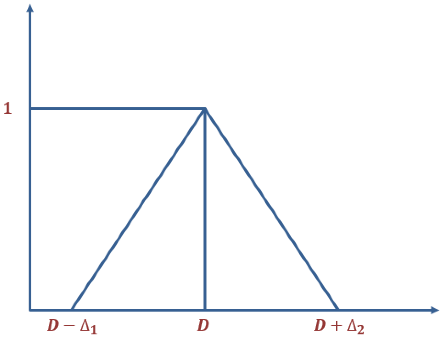
Cárdenas-Barrón [14] viewed annual demand as a constant parameter. However, in several real world scenarios, some uncertainties may alter annual demand slightly. Thus, annual demand may be considered as a fuzzy number. To replace the annual demand D by a fuzzy number D ˜ , consider the fuzzy number D ˜ as a TFN D ˜ = ( D Δ 1 , D , D + Δ 2 ) , where 0 < Δ 1 < D and 0 < Δ 2 as shown in Figure 4. The Fuzzy Membership Function (FMF) of D ˜ is formulated as
μ D ˜ ( x ) = { x D + Δ 1 Δ 1             i f               D Δ 1 x D D + Δ 2 x Δ 2             i f               D x D + Δ 2 0      o t h e r w i s e   .                    
The centroid of μ D ˜ ( x ) is given by D = D + 1 3 ( Δ 2 Δ 1 ) . This result is considered to obtain the annual demand in fuzzy sense. For any T > 0 , let T C ( Q )   ( x ) = y ( > 0 ) . Using the extension principle of Kaufmann and Gupta [63] and Zimmermann [64], the membership function of the fuzzy cost T C ( Q ) ( D ˜ ) is formulated as
μ T C ( Q ) D ˜ ( y ) = { s u p x ϵ T C ( Q ) 1 ( y ) μ ( D ˜ ) ( x )       i f         T C ( Q ) 1 ( y ) 0     i f         T C ( Q ) 1 ( y ) = .
From T C ( Q )   ( x ) = y and the system cost function, we obtain
y = ( Q 2 ( H P n D H ( 1 + α n + α n 2 ) ) + 2 D P n i = 1 n K i + 2 D Q P n ( i = 1 n C i ( 1 + α i ) + i = 1 n J i ( 1 + α i ) ) ) 2 Q P n ( 1 + ρ ) ( 1 + D k = 1 n 1 ( 1 + α k P k ) )
For simplification purpose, let us assume
B = H P n ,
F = H ( 1 + α n + α n 2 ) ,
L = 2 P n i = 1 n K i ,
G = 2 P n ( i = 1 n C i ( 1 + α i ) + i = 1 n J i ( 1 + α i ) ) ,
M = 2 P n ( 1 + ρ ) ,
and
R = 2 P n ( 1 + ρ ) k = 1 n 1 ( 1 + α k P k ) .
This provides
y = B Q 2 + D ( L + Q ( G F Q ) ) Q ( M + D R )
and
x = Q ( B Q M y ) F Q 2 + Q R y L G Q
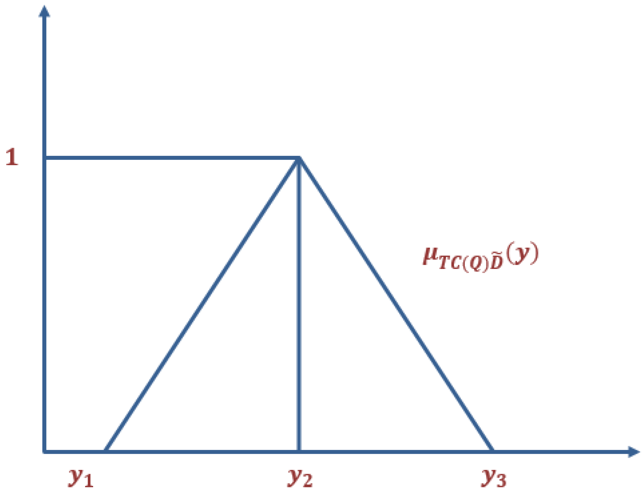
From the standard triangular FMF and values of x and   y , the FMF of T C ( Q ) ( D ˜ ) is given by
μ T C ( Q ) D ˜ ( y ) = { Q ( B Q M y ) ( F Q 2 + Q R y L G Q ) Δ 1 D Δ 1 Δ 1       i f       y 1 y y 2   D + Δ 2 Δ 2 Q ( B Q M y ) ( F Q 2 + Q R y L G Q ) Δ 2         i f       y 2 y y 3 .
Figure 5 represents the FMF of T C ( Q ) ( D ˜ ) .
Now centroid of   μ T C ( Q ) D ˜ ( y ) is formulated as
T C ( Q ) = [ y μ T C ( Q ) D ˜ ( y ) ] d y [ μ T C ( Q ) D ˜ ( y ) ] d y
After defuzzification, crisp total cost function becomes
T C ( Q ) = ( B Q 2 + D ( L + Q ( G F Q ) ) M + D R + B Q 2 + ( L + Q ( G F Q ) ) ( D Δ 1 ) M + R ( D Δ 1 ) + B Q 2 + ( L + Q ( G F Q ) ) ( D + Δ 2 ) M + R ( D + Δ 2 ) ) 3 Q
As lot size Q is a decision variable, we differentiate the cost function (17) with respect to Q. Thus, from the necessary conditions, we have
d ( T C ) d Q = ( Δ 1 ( ( M + D R ) ( L ( M + 3 D R ) + Q 2 ( F M 2 B R + 3 D F R ) ) + R ( L ( 2 M + 3 D R ) + Q 2 ( 2 F M B R + 3 D F R ) ) Δ 2 ) ( M + D R ) ( 3 ( B Q 2 + D ( L + F Q 2 ) ) ( M + D R ) + ( L ( M + 3 D R ) + Q 2 ( F M 2 B R + 3 D F R ) ) Δ 2 ) ) 3 Q 2 ( M + D R ) ( M + D R R Δ 1 ) ( M + D R + R Δ 2 ) = 0
After some simplification, Equation (18) can be written in standard quadratic form as
d ( T C ) d Q = ( L ( ( M + d R ) ( 3 d ( M + d R ) + ( M + 3 d R ) Δ 2 ) + Δ 1 ( ( M + d R ) ( M + 3 d R ) + R ( 2 M + 3 d R ) Δ 2 ) ) + Q 2 ( Δ 1 ( ( M + d R ) ( F M 2 B R + 3 d F R ) + R ( 2 F M B R + 3 d F R ) Δ 2 ) + ( M + d R )   ( 3 ( B d F ) ( M + d R ) + ( 2 B R F ( M + 3 d R ) ) Δ 2 ) ) ) 3 Q 2 ( M + d R ) ( M + d R R Δ 1 ) ( M + d R + R Δ 2 ) = 0
Quadratic equation (19) provide two roots, one is negative and the other is positive. It is a well-known fact that quadratic equation has only one positive root. Thus, the two solutions for the optimal lot size are obtained as below
Q = ± ( L ( ( M + D R ) ( 3 D ( M + D R ) + ( M + 3 D R ) Δ 2 ) Δ 1 ( ( M + D R ) ( M + 3 D R ) + R Δ 2 ( 2 M + 3 D R ) ) ) ( Δ 1 ( ( M + D R ) ( F M 2 B R + 3 D F R ) + R Δ 2 ( 2 F M B R + 3 D F R ) ) + ( M + D R ) ( 3 ( B D F ) ( M + D R ) + ( 2 B R F ( M + 3 D R ) ) Δ 2 ) ) )
Negative root seems quite impossible candidate solution for optimal lot size problem, and is thus discarded. The positive root is taken as the optimal lot size Q ,
Q = ( L ( ( M + D R ) ( 3 D ( M + D R ) + ( M + 3 D R ) Δ 2 ) Δ 1 ( ( M + D R ) ( M + 3 D R ) + R Δ 2 ( 2 M + 3 D R ) ) ) ( Δ 1 ( ( M + D R ) ( F M 2 B R + 3 D F R ) + R Δ 2 ( 2 F M B R + 3 D F R ) ) + ( M + D R ) ( 3 ( B D F ) ( M + D R ) + ( 2 B R F ( M + 3 D R ) ) Δ 2 ) ) )
To satisfy sufficient conditions,
d 2 ( T C ) ( d Q ) 2 = 2 L ( 3 + M ( 1 M + D R 1 M + D R R Δ 1 1 M + D R + R Δ 2 ) ) 3 Q 3 R > 0
As the solution to the above expression is positive, the sufficient condition is also satisfied. Thus the system cost attains minimum value in the interval (0, T) for Q*.

3. Numerical Experiment and Results

This section analyzes the impact of various numerical values of parameters on the optimal cost of the system by taking appropriate units. Three numerical experiments are carried out for a five-stage production system ( n = 5 ) .

3.1. Example 1

Parameters K i = $ 100 /stage, D = 50,000 items/year, P n = 200,000 items/year, H = $ 5 /item/year, and ρ = 2.00 % per stage are taken from Wee et al. [37] and Biswas and Sarker [19]. Parameters α i = 1.00 % for each stage, C i = $ 3 /item for each stage, J i = $ 0.02 /item for each stage, P n 1 = 210,000 items/year, P n 2 = 220,500 items/year, P n 3 = 231,525 items/year, P n 4 = 243,102 items/year, and Δ 1 = 8000 , and Δ 2 = 12,000 are considered randomly.

3.2. Example 2

Numerical values of the parameters in this example are taken from Tayyab and Sarkar [61] as K i = $ 400 /stage, D = 15,000 items/year, P n = 70,000 items/year, H = $ 4 /item/year, ρ = 2.00 % per stage, C i = $ 35 /item for each stage, J i = $ 1 /item for each stage, P n 1 = 73,500 items/year, P n 2 = 77,175 items/year, P n 3 = 81,033 items/year, P n 4 = 85,085 items/year, and α i = 1.00 % for each production stage is the same as in Example 1. Parameters Δ 1 = 3000 and Δ 2 = 4000 are considered randomly.

3.3. Example 3

Numerical values of the parameters in this example are taken from Tayyab and Sarkar [61] as K i = $ 200 /stage, D = 12,000 items/year, P n = 60,000 items/year, H = $ 20 /item/year, ρ = 2.00 % per stage, C i = $ 100 /item for each stage, J i = $ 0.5 /item for each stage, P n 1 = 63,000 items/year, P n 2 = 66,150 items/year, P n 3 = 69,457 items/year, P n 4 = 72,930 items/year, and α i = 1.00 % for each production stage is same as in Example 1 and 2. Parameters Δ 1 = 2000 and Δ 2 = 3000 are considered randomly.
Optimal results of the above numerical examples are provided in Table 1.

4. Discussion

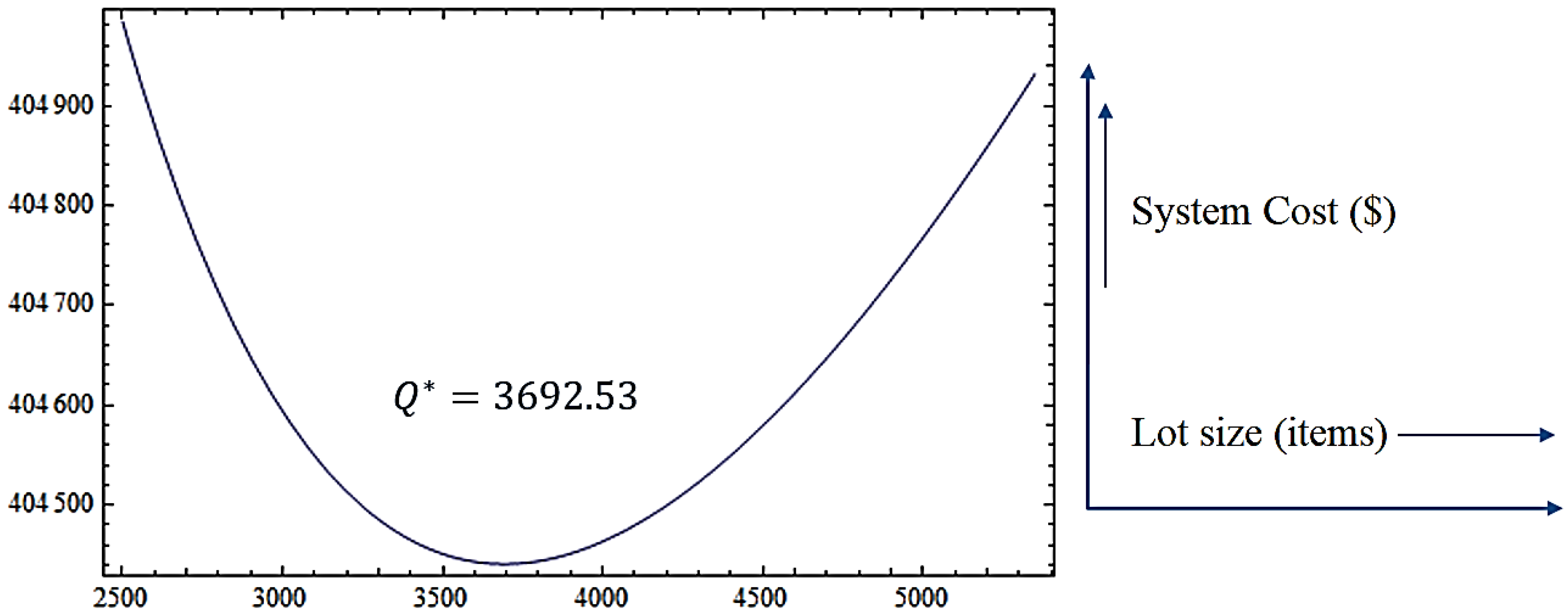
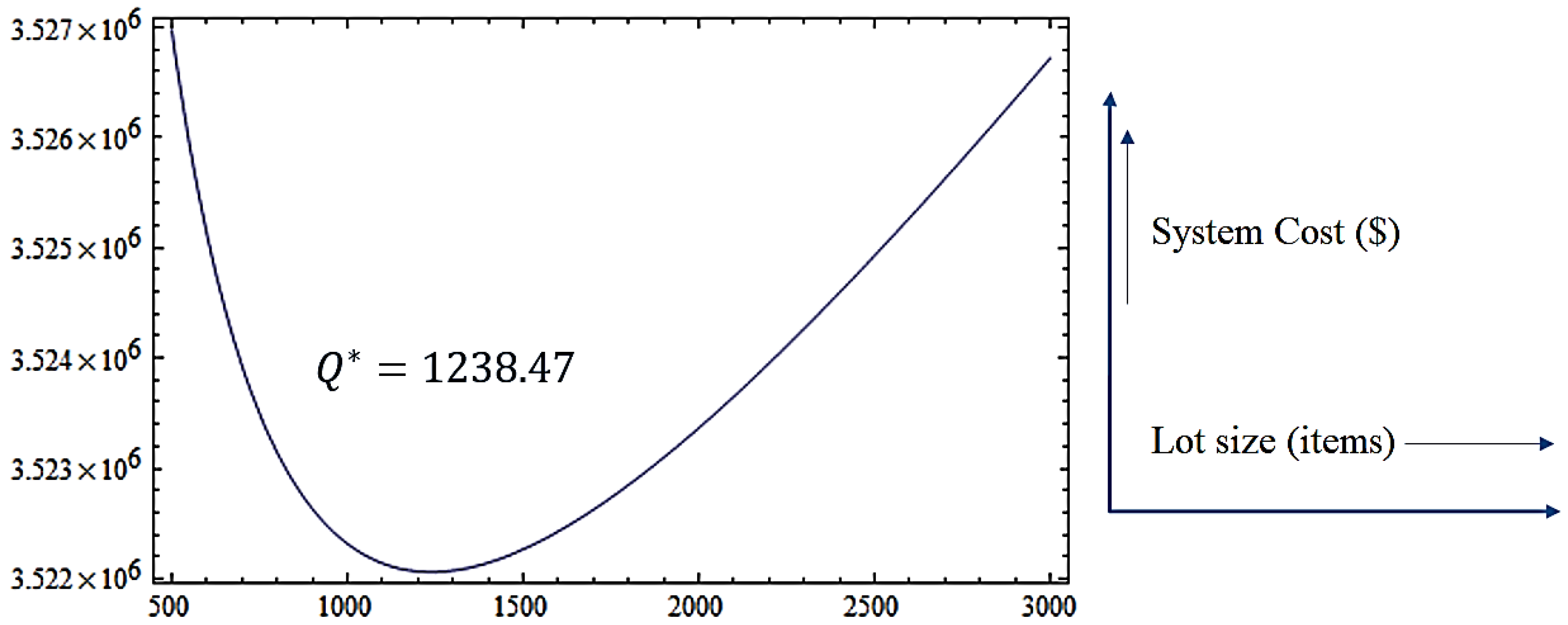
Decision makers of the multi-stage production systems can get the advantage of the proposed production model to reduce system cost in the presence of defective production and imprecise information. The proposed production model has provided global optimal results for lot size decision to achieve the minimum cost of the multi-stage production system. The detailed procedure of fuzzy theory application provided for uncertainty control can enable the managers and decision-makers to conveniently address the uncertain conditions of respective shop-floors. Each numerical example is solved for five-stage production systems and results are summarized in Table 1. Figure 6, Figure 7 and Figure 8 illustrate the convexity of minimum cost objective in each case, which verifies the robustness of the model. Optimal results indicate that the larger lot sizes provide more benefit to the production systems comprising of higher number of stages. For instance, in Example 3, optimal lot size for single-stage production system is 557.94 items and 1238.47 items for five-stage production system. Consistency in the obtained results assures that this research work has achieved the desired goal of analyzing product imperfection and imprecise information in multi-stage production modeling.
Optimal results are further evaluated for the possible variations in key parameters of the given examples. The effect of key parameters on the optimal cost function for up-to five-stage production system is summarized in Table 2, Table 3 and Table 4 for Example 1 to Example 3, respectively. The values of the parameters are varied from −50% to +50%.
  • It is evident from the change in optimal cost function that the order processing cost ( C i ) is the most sensitive factor than other parameters. One can observe that with each percentage increase in C i there exists almost similar amount of percentage increase in the system cost. For instance, regarding four-stage production system in Example 2, system cost increases by 24.17% by the increment of 25% in order of processing cost, and 48.34% increase in system cost is observed by a 50% rise in the order of processing cost.
  • Next to the effect of order processing cost is the impact of production rate ( P i ) on the system cost. It can be noted that the effect of production rate on the production system with higher number of stages is more than the system with a lower number of production stages. This illustrates the necessity of wisely adjusting production rate at each production stage to keep the system cost at its minimum value.
  • An interesting observation from the sensitivity analysis of all the numerical examples reveal that the impact of setup cost ( K i ) and the inventory holding cost ( H ) is same on the system cost for all the production systems with any number of stages. Thus, the decision makers have to make intelligent decision in putting efforts to reduce one of these costs first. Here arises the importance of lean philosophy, as Single Minute Exchange of Dyes (SMED) is the best possible solution for setup cost reduction. Therefore, managers should make efforts to apply SMED for setup cost reduction first, as it is much more beneficial than cutting down stock management equipment and inventory holding staff.
  • Inspection cost ( J i ) and defective proportion ( α i ) bear trivial impact on the system cost that gradually varies as the system moves towards a higher number of stages.
The sensitivity analysis provides important inferences for the managers to develop optimal policies that can achieve the best outcomes at their shop floors.

5. Conclusions

Agreeing to lean philosophy, high inventory levels are considered as one of the major non-value added aspect of the production system. For true implementation of lean culture, inventory as a form of non-value added activity should be reduced to its minimum. Therefore, there must be a defined optimal lot size in accordance with the input requirements of each production stage at minimum system cost. Cárdenas-Barrón [14] provided interpretation of considering defective rate in his inventory model to achieve optimal cost at the single-stage production facility. This inference is carried forward in this paper for its implication on a multi-stage production system.
This study is made-up to support production and planning managers, especially in the textile production sector where defective production and uncertain product demand are faced. It introduces an imperfect multi-stage production model with the consideration of defective proportion in the production process and uncertain product demand. Thus, the novelty of this study is the introduction of imperfect production proportion at each stage of the multi-stage production system and imprecise product demand. Fuzzy theory is applied to handle the uncertainty in demand information and center of gravity approach is utilized to defuzzify the objective function. This defuzzified cost objective is solved through the analytical optimization technique and closed form solution of the optimal lot size is obtained.
Numerical experiment comprising of three examples is conducted and optimal results are analyzed through sensitivity analysis. Optimal results indicate that as the number of stages increase, lots of larger sizes are cost effective. Sensitivity analysis indicates that the order processing cost bears the highest effect on the system cost and its effect increases slightly as the system moves towards higher number of stages. Creditably, this study can work as an elementary support in implementing lean culture in the production system. Analysis of the model illustrates the major advantage of this study by highlighting the importance of lean activities to reduce the system cost, as the results suggest application of SMED for setup cost reduction in the multi-stage production system prior to making efforts for inventory holding cost reduction.
Despite various benefits, this study has some limitations. It has considered constant defective proportion in the production system, whereas defective rate becomes imprecise in long run production processes. Secondly, the proposed model has incorporated a perfect reworking opportunity that is very rare in the real life production systems, as defective products are also produced during reworking. The analysis of the results state that the effect of order processing cost on the total system cost is highest among all other system parameters. However, this study has not provided order processing cost reduction policy to minimize system cost for future runs. Further, the model can be extended with several ideas including consideration of shortages backordered [39,65,66], variable production rate [67,68,69], trade credit policies [70,71], allocation problem [72,73], and different rework options [19]. The immediate possible extension to this paper can be the incorporation of uncertain defective rate [61,62].

Author Contributions

Conceptualization, M.T. and B.S.; Methodology, M.T.; Software, M.T.; Validation, B.S.; Formal analysis, M.T. and B.S.; Investigation, M.T.; Resources, M.T. B.S. and B.N.Y.; Data curation, M.T. and B.S.; Writing—original draft preparation, M.T.; Writing—review and editing, B.S. and B.N.Y.; Visualization, M.T. B.S. and B.N.Y.; Supervision, B.S.

Funding

This research received no external funding.

Conflicts of Interest

The authors declare no conflict of interest.

Nomenclature

Indices
kproduction stages (k = 1, 2, 3… (n − 1))
iproduction stages (i = 1, 2, 3… n)
Decision variable
Qlot size (items)
Parameters
n number of production stages
P k production rate for k t h production stage (items per unit time)
P n production rate for n t h production stage (items per unit time, where P k > P n > D )
D ˜ demand rate (fuzzy, and fulfilled at n t h production stage)
α k defective proportion at k t h production stage
α n defective proportion at n t h production stage
T k cycle time of k t h production stage (years)
T n cycle time of n t h production stage (years)
T time between production runs (total cycle time of n -stages, years)
K i setup cost of i t h production stage ($/setup)
H inventory holding cost of finished items ($/item/year)
C i order processing cost at i t h production stage ($/item/stage)
J i inspection cost at i t h production stage ($/item/stage)
ρ percentage setup time per stage
I ¯ average inventory of finished items in the system
T C ( Q ) total cost of the production system ($ per unit time)

Abbreviations

Below enlisted abbreviations are used for the multi-stage production model development in this research work.
EOQEconomic order quantity
EPQEconomic production quantity
TFNTriangular fuzzy number
FMFFuzzy membership function
SMEDSingle minute exchange of dyes

References

  1. Hodge, G.L.; Goforth Ross, K.; Joines, J.A.; Thoney, K. Adapting lean manufacturing principles to the textile industry. Prod. Plan. Control 2011, 22, 237–247. [Google Scholar] [CrossRef]
  2. Harris, F.W. How many parts to make at once. Fact. Mag. Manag. 1913, 10, 135–136. [Google Scholar] [CrossRef]
  3. Taft, E.W. The most economical production lot. Iron Age 1918, 101, 1410–1412. [Google Scholar]
  4. Lee, H.L. Lot sizing to reduce capacity utilization in a production process with defective items, process corrections, and rework. Manag. Sci. 1992, 38, 1314–1328. [Google Scholar] [CrossRef]
  5. Gupta, T.; Chakraborty, S. Looping in a multistage production system. Int. J. Prod. Res. 1984, 22, 299–311. [Google Scholar] [CrossRef]
  6. Tayi, G.K.; Ballou, D.P. An integrated production-inventory model with reprocessing and inspection. Int. J. Prod. Res. 1988, 26, 1299–1315. [Google Scholar] [CrossRef]
  7. Lee, H.H.; Chandra, M.J.; Deleveaux, V.J. Optimal batch size and investment in multistage production systems with scrap. Prod. Plan. Control 1997, 8, 586–596. [Google Scholar] [CrossRef]
  8. Glock, C.H.; Jaber, M.Y. Learning effects and the phenomenon of moving bottlenecks in a two-stage production system. Appl. Math. Model. 2013, 37, 8617–8628. [Google Scholar] [CrossRef]
  9. Lin, C.S. Integrated production-inventory models with imperfect production processes and a limited capacity for raw materials. Math. Comput. Model. 1999, 29, 81–89. [Google Scholar] [CrossRef]
  10. Salameh, M.K.; Jaber, M.Y. Economic production quantity model for items with imperfect quality. Int. J. Prod. Econ. 2000, 64, 59–64. [Google Scholar] [CrossRef]
  11. Khan, M.; Jaber, M.Y.; Guiffrida, A.L.; Zolfaghari, S. A review of the extensions of a modified EOQ model for imperfect quality items. Int. J. Prod. Econ. 2011, 132, 1–2. [Google Scholar] [CrossRef]
  12. Jaber, M.Y.; Zanoni, S.; Zavanella, L.E. Economic order quantity models for imperfect items with buy and repair options. Int. J. Prod. Econ. 2014, 155, 126–131. [Google Scholar] [CrossRef]
  13. Ouyang, L.Y.; Chen, C.K.; Chang, H.C. Quality improvement, setup cost and lead-time reductions in lot size reorder point models with an imperfect production process. Comput. Oper. Res. 2002, 29, 1701–1717. [Google Scholar] [CrossRef]
  14. Cárdenas-Barrón, L.E. Economic production quantity with rework process at a single-stage manufacturing system with planned backorders. Comput. Ind. Eng. 2009, 57, 1105–1113. [Google Scholar] [CrossRef]
  15. Eroglu, A.; Ozdemir, G. An economic order quantity model with defective items and shortages. Int. J. Prod. Econ. 2007, 106, 544–549. [Google Scholar] [CrossRef]
  16. Jaber, M.Y.; Guiffrida, A.L. Learning curves for imperfect production processes with reworks and process restoration interruptions. Eur. J. Oper. Res. 2008, 189, 93–104. [Google Scholar] [CrossRef]
  17. Ben-Daya, M. The economic production lot-sizing problem with imperfect production processes and imperfect maintenance. Int. J. Prod. Econ. 2002, 76, 257–264. [Google Scholar] [CrossRef]
  18. Jamal, A.M.; Sarker, B.R.; Mondal, S. Optimal manufacturing batch size with rework process at a single-stage production system. Comput. Ind. Eng. 2004, 47, 77–89. [Google Scholar] [CrossRef]
  19. Biswas, P.; Sarker, B.R. Optimal batch quantity models for a lean production system with in-cycle rework and scrap. Int. J. Prod. Res. 2008, 46, 6585–6610. [Google Scholar] [CrossRef]
  20. Chung, K.J. The economic production quantity with rework process in supply chain management. Comput. Math. Appl. 2011, 62, 2547–2550. [Google Scholar] [CrossRef]
  21. Taleizadeh, A.A.; Jalali-Naini, S.G.; Wee, H.M.; Kuo, T.C. An imperfect multi-product production system with rework. Sci. Iran 2013, 20, 811–823. [Google Scholar]
  22. Cárdenas-Barrón, L.E. Optimal manufacturing batch size with rework in a single-stage production system—A simple derivation. Comput. Ind. Eng. 2008, 55, 758–765. [Google Scholar] [CrossRef]
  23. Ma, W.N.; Gong, D.C.; Lin, G.C. An optimal common production cycle time for imperfect production processes with scrap. Math. Comput. Model. 2010, 52, 724–737. [Google Scholar] [CrossRef]
  24. Barzoki, M.R.; Jahanbazi, M.; Bijari, M. Effects of imperfect products on lot sizing with work in process inventory. Appl. Math. Comput. 2011, 217, 8328–8336. [Google Scholar] [CrossRef]
  25. Chiu, S.W.; Tseng, C.T.; Wu, M.F.; Sung, P.C. Multi-item EPQ model with scrap, rework and multi-delivery using common cycle policy. J. Appl. Res. Technol. 2014, 12, 615–622. [Google Scholar] [CrossRef]
  26. Chiu, S.W.; Chiu, Y.S.; Yang, J.C. Combining an alternative multi-delivery policy into economic production lot size problem with partial rework. Expert Syst. Appl. 2012, 39, 2578–2583. [Google Scholar] [CrossRef]
  27. Noorollahi, E.; Karimi-Nasab, M.; Aryanezhad, M.B. An economic production quantity model with random yield subject to process compressibility. Math. Comput. Model. 2012, 56, 80–96. [Google Scholar] [CrossRef]
  28. Moussawi-Haidar, L.; Salameh, M.; Nasr, W. Production lot sizing with quality screening and rework. Appl. Math. Model. 2016, 40, 3242–3256. [Google Scholar] [CrossRef]
  29. Chiu, S.W.; Gong, D.C.; Wee, H.M. Effects of random defective rate and imperfect rework process on economic production quantity model. Jpn. J. Ind. Appl. Math. 2004, 21, 375. [Google Scholar] [CrossRef]
  30. Taleizadeh, A.A.; Cárdenas-Barrón, L.E.; Mohammadi, B. A deterministic multi product single machine EPQ model with backordering, scraped products, rework and interruption in manufacturing process. Int. J. Prod. Econ. 2014, 150, 9–27. [Google Scholar] [CrossRef]
  31. Chiu, S.W.; Ting, C.K.; Chiu, Y.S. Optimal production lot sizing with rework, scrap rate, and service level constraint. Math. Comput. Model. 2007, 46, 535–549. [Google Scholar] [CrossRef]
  32. Taleizadeh, A.A.; Wee, H.M.; Jalali-Naini, S.G. Economic production quantity model with repair failure and limited capacity. Appl. Math. Model. 2013, 37, 2765–2774. [Google Scholar] [CrossRef]
  33. Sana, S.S. A production–inventory model in an imperfect production process. Eur. J. Oper. Res. 2010, 200, 451–464. [Google Scholar] [CrossRef]
  34. Sarkar, B.; Moon, I. An EPQ model with inflation in an imperfect production system. Appl. Math. Comput. 2011, 217, 6159–6167. [Google Scholar] [CrossRef]
  35. Yoo, S.H.; Kim, D.; Park, M.S. Lot sizing and quality investment with quality cost analyses for imperfect production and inspection processes with commercial return. Int. J. Prod. Econ. 2012, 140, 922–933. [Google Scholar] [CrossRef]
  36. Chakraborty, T.; Giri, B.C. Joint determination of optimal safety stocks and production policy for an imperfect production system. Appl. Math. Model. 2012, 36, 712–722. [Google Scholar] [CrossRef]
  37. Wee, H.M.; Wang, W.T.; Yang, P.C. A production quantity model for imperfect quality items with shortage and screening constraint. Int. J. Prod. Res. 2013, 51, 1869–1884. [Google Scholar] [CrossRef]
  38. Chiu, S.W.; Chou, C.L.; Wu, W.K. Optimizing replenishment policy in an EPQ-based inventory model with nonconforming items and breakdown. Econ. Model. 2013, 35, 330–337. [Google Scholar] [CrossRef]
  39. Sarkar, B.; Cárdenas-Barrón, L.E.; Sarkar, M.; Singgih, M.L. An economic production quantity model with random defective rate, rework process and backorders for a single stage production system. J. Manuf. Syst. 2014, 33, 423–435. [Google Scholar] [CrossRef]
  40. Dang, J.F.; Hong, I.H. The Cournot game under a fuzzy decision environment. Comput. Math. Appl. 2010, 59, 3099–3109. [Google Scholar] [CrossRef]
  41. Zadeh, L.A. Fuzzy sets as a basis for a theory of possibility. Fuzzy Set Syst. 1999, 100, 9–34. [Google Scholar] [CrossRef]
  42. Petrovic, D.; Sweeney, E. Fuzzy knowledge-based approach to treating uncertainty in inventory control. Comput. Integr. Manuf. Syst. 1994, 7, 147–152. [Google Scholar] [CrossRef] [Green Version]
  43. Roy, T.K.; Maiti, M. Multi-objective inventory models of deteriorating items with some constraints in a fuzzy environment. Comput. Oper. Res. 1998, 25, 1085–1095. [Google Scholar] [CrossRef]
  44. Yao, J.S.; Chang, S.C.; Su, J.S. Fuzzy inventory without backorder for fuzzy order quantity and fuzzy total demand quantity. Comput. Oper. Res. 2000, 27, 935–962. [Google Scholar] [CrossRef]
  45. Chang, H.C.; Yao, J.S.; Ouyang, L.Y. Fuzzy mixture inventory model involving fuzzy random variable lead time demand and fuzzy total demand. Eur. J. Oper. Res. 2006, 169, 65–80. [Google Scholar] [CrossRef]
  46. Mahata, G.C.; Goswami, A. Fuzzy inventory models for items with imperfect quality and shortage backordering under crisp and fuzzy decision variables. Comput. Ind. Eng. 2013, 64, 190–199. [Google Scholar] [CrossRef]
  47. De, S.K.; Goswami, A.; Sana, S.S. An interpolating by pass to Pareto optimality in intuitionistic fuzzy technique for a EOQ model with time sensitive backlogging. Appl. Math. Comput. 2014, 230, 664–674. [Google Scholar] [CrossRef]
  48. Chang, S.Y.; Yeh, T.Y. A two-echelon supply chain of a returnable product with fuzzy demand. Appl. Math. Model. 2013, 37, 4305–4315. [Google Scholar] [CrossRef]
  49. Sadeghi, J.; Niaki, S.T. Two parameter tuned multi-objective evolutionary algorithms for a bi-objective vendor managed inventory model with trapezoidal fuzzy demand. Appl. Soft Comput. 2015, 30, 567–576. [Google Scholar] [CrossRef]
  50. Lin, J.; Hung, K.C.; Julian, P. Technical note on inventory model with trapezoidal type demand. Appl. Math. Model. 2014, 38, 4941–4948. [Google Scholar] [CrossRef]
  51. Coşgun, Ö.; Ekinci, Y.; Yanık, S. Fuzzy rule-based demand forecasting for dynamic pricing of a time company. Knowl. Based Syst. 2014, 70, 88–96. [Google Scholar] [CrossRef]
  52. Sadeghi, J.; Mousavi, S.M.; Niaki, S.T. Optimizing an inventory model with fuzzy demand, backordering, and discount using a hybrid imperialist competitive algorithm. Appl. Math. Model. 2016, 40, 7318–7335. [Google Scholar] [CrossRef]
  53. Rong, M.; Maiti, M. On an EOQ model with service level constraint under fuzzy-stochastic demand and variable lead-time. Appl. Math. Model. 2015, 39, 5230–5240. [Google Scholar] [CrossRef]
  54. Zhang, B.; Lu, S.; Zhang, D.; Wen, K. Supply chain coordination based on a buyback contract under fuzzy random variable demand. Fuzzy Set Syst. 2014, 255, 1–6. [Google Scholar] [CrossRef]
  55. Moghaddam, K.S. Fuzzy multi-objective model for supplier selection and order allocation in reverse logistics systems under supply and demand uncertainty. Expert Syst. Appl. 2015, 42, 6237–6254. [Google Scholar] [CrossRef]
  56. Huang, M.; Song, M.; Leon, V.J.; Wang, X. Dentralized capacity allocation of a single-facility with fuzzy demand. J. Manuf. Syst. 2014, 33, 7–15. [Google Scholar] [CrossRef]
  57. Taleizadeh, A.A.; Niaki, S.T.; Nikousokhan, R. Constraint multiproduct joint-replenishment inventory control problem using uncertain programming. Appl. Soft Comput. 2011, 11, 5143–5154. [Google Scholar] [CrossRef]
  58. Jana, D.K.; Das, B.; Maiti, M. Multi-item partial backlogging inventory models over random planninghorizon in random fuzzy environment. Appl. Soft Comput. 2014, 21, 12–27. [Google Scholar] [CrossRef]
  59. Das, B.C.; Das, B.; Mondal, S.K. An integrated production inventory model under interactive fuzzy credit period for deteriorating item with several kets. Appl. Soft Comput. 2015, 28, 453–465. [Google Scholar] [CrossRef]
  60. Ku, R.S.; Goswami, A. A fuzzy random EPQ model for imperfect quality items with possibility and necessity constraints. Appl. Soft Comput. 2015, 34, 838–850. [Google Scholar]
  61. Tayyab, M.; Sarkar, B. Optimal batch quantity in a cleaner multi-stage lean production system with random defective rate. J. Clean. Prod. 2016, 139, 922–934. [Google Scholar] [CrossRef]
  62. Kim, M.S.; Sarkar, B. Multi-stage cleaner production process with quality improvement and lead time dependent ordering cost. J. Clean. Prod. 2017, 144, 572–590. [Google Scholar] [CrossRef]
  63. Kaufman, A.; Gupta, M.M. Introduction to Fuzzy Arithmetic; Van Nostrand Reinhold Company: New York, NY, USA, 1991. [Google Scholar]
  64. Zimmermann, H.J. Fuzzy control. In Fuzzy Set Theory—And Its Applications; Springer: Dordrecht, The Netherlands, 1996; pp. 203–240. [Google Scholar]
  65. Sarkar, B.; Moon, I. Improved quality, setup cost reduction, and variable backorder costs in an imperfect production process. Int. J. Prod. Econ. 2014, 155, 204–213. [Google Scholar] [CrossRef]
  66. Sarkar, B. A production-inventory model with probabilistic deterioration in two-echelon supply chain management. Appl. Math. Model. 2013, 37, 3138–3151. [Google Scholar] [CrossRef]
  67. Sarkar, B.; Sana, S.S.; Chaudhuri, K. Optimal reliability, production lotsize and safety stock: An economic manufacturing quantity model. Int. J. Manag. Sci. Eng. Manag. 2010, 5, 192–202. [Google Scholar] [CrossRef]
  68. Moon, I.; Shin, E.; Sarkar, B. Min–max distribution free continuous-review model with a service level constraint and variable lead time. Appl. Math. Comput. 2014, 229, 310–315. [Google Scholar] [CrossRef]
  69. Shin, D.; Guchhait, R.; Sarkar, B.; Mittal, M. Controllable lead time, service level constraint, and transportation discounts in a continuous review inventory model. Rairo-Oper. Res. 2016, 50, 921–934. [Google Scholar] [CrossRef]
  70. Sarkar, B.; Ahmed, W.; Kim, N. Joint effects of variable carbon emission cost and multi-delay-in-payments under single-setup-multiple-delivery policy in a global sustainable supply chain. J. Clean. Prod. 2018, 185, 421–445. [Google Scholar] [CrossRef]
  71. Sarkar, B.; Sana, S.S.; Chaudhuri, K. An inventory model with finite replenishment rate, trade credit policy and price-discount offer. J. Ind. Eng. 2013, 1–18. [Google Scholar] [CrossRef]
  72. Ahmed, W.; Sarkar, B. Impact of carbon emissions in a sustainable supply chain management for a second generation biofuel. J. Clean. Prod. 2018, 186, 807–820. [Google Scholar] [CrossRef]
  73. Cárdenas-barrón, L.E.; Sarkar, B.; Treviño-garza, G. Easy and improved algorithms to joint determination of the replenishment lot size and number of shipments for an EPQ model with rework. Math. Comput. Appl. 2013, 18, 132–138. [Google Scholar] [CrossRef]
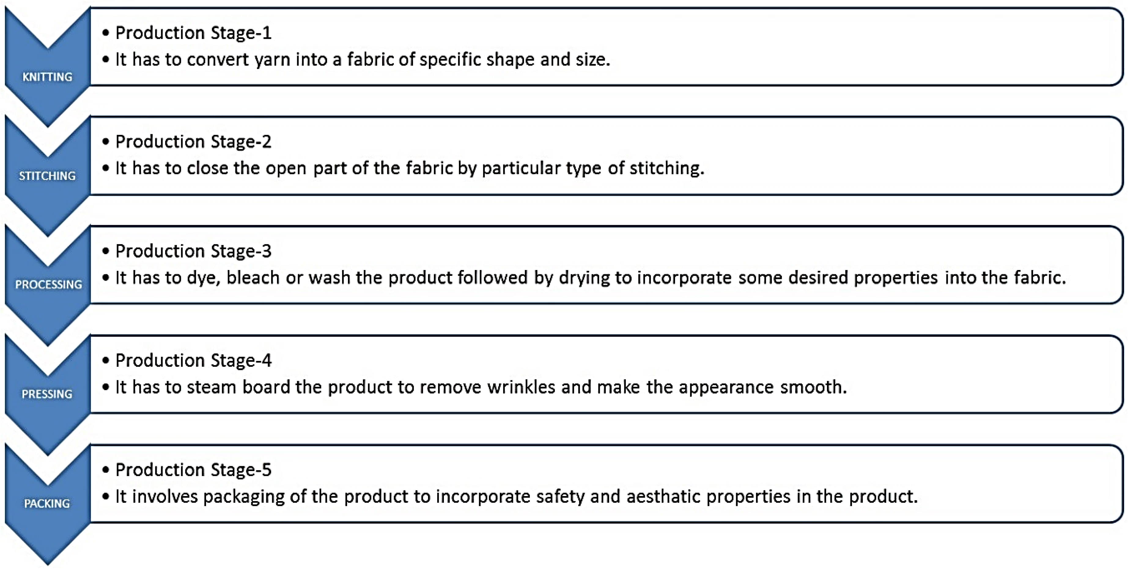
Figure 1. General production flow of an apparel manufacturing industry.
Mathematics 07 00013 g001
Figure 2. Inventory diagram of k t h production stage.
Mathematics 07 00013 g002
Figure 3. Inventory diagram of n t h production stage.
Mathematics 07 00013 g003
Figure 4. Triangular fuzzy number D ˜ .
Mathematics 07 00013 g004
Figure 5. Triangular fuzzy number T C ( Q ) ( D ˜ ) .
Mathematics 07 00013 g005
Figure 6. Objective function convexity diagram for Example 1 (Five-stage production system).
Mathematics 07 00013 g006
Figure 7. Objective function convexity diagram for Example 2 (Five-stage production system).
Mathematics 07 00013 g007
Figure 8. Objective function convexity diagram for Example 3 (Five-stage production system).
Mathematics 07 00013 g008
Table 1. Optimal results of the numerical experiments.
Production StagesExample 1Example 2Example 3
Q* (items)TC* ($)Q* (items)TC* ($)Q* (items)TC* ($)
Single-stage1664.93159,5521984.44552,648557.941,236,016
Two-stage2346.56252,0802795.5905,477786.792,051,893
Three-stage2867.7316,0703414.821,160,906961.722,652,656
Four-stage3306.35364,8083935.671,360,7731108.923,127,405
Five-stage3692.53404,4414393.981,525,9501238.473,522,058
Table 2. Sensitivity analysis of key parameters for Example 1.
ParametersChange (%) Percentage Change in TC(Q)*
Single-Stage ProcessTwo-Stage ProcessThree-Stage ProcessFour-Stage ProcessFive-Stage Process
P i −50−0.73−17.09−24.92−29.53−32.57
−25−0.23−6.41−9.94−12.24−13.85
+25+0.13+4.27+7.09+9.13+10.67
+50+0.21+7.33+12.40+16.20+19.15
K i −50−1.11−0.80−0.65−0.57−0.51
−25−0.51−0.36−0.30−0.26−0.23
+25+0.45+0.32+0.26+0.23+0.21
+50+0.85+0.61+0.50+0.44+0.39
C i −50−47.79−48.32−48.56−48.70−48.80
−25−23.89−24.16−24.28−24.35−24.40
+25+23.89+24.16+24.28+24.35+24.40
+50+47.79+48.32+48.56+48.70+48.80
J i −50−0.32−0.32−0.32−0.32−0.33
−25−0.16−0.16−0.16−0.16−0.16
+25+0.16+0.16+0.16+0.16+0.16
+50+0.32+0.32+0.32+0.32+0.33
H −50−1.11−0.80−0.65−0.57−0.51
−25−0.51−0.36−0.30−0.26−0.23
+25+0.45+0.32+0.26+0.23+0.21
+50+0.85+0.61+0.50+0.44+0.39
α i −50−0.47−0.38−0.32−0.28−0.25
−25−0.24−0.19−0.16−0.14−0.12
+25+0.24+0.19+0.16+0.14+0.12
+50+0.47+0.38+0.32+0.28+0.25
Table 3. Sensitivity analysis of key parameters for Example 2.
ParametersChange (%) Percentage Change in TC(Q)*
Single-Stage ProcessTwo-Stage ProcessThree-Stage ProcessFour-Stage ProcessFive-Stage Process
P i −50−0.17−15.12−22.75−27.42−30.57
−25−0.05−5.61−8.95−11.20−12.81
+25+0.03+3.70+6.28+8.20+9.69
+50+0.05+6.33+10.94+14.48+17.28
K i −50−0.32−0.23−0.19−0.16−0.15
−25−0.15−0.10−0.09−0.07−0.07
+25+0.13+0.09+0.08+0.07+0.06
+50+0.25+0.18+0.14+0.12+0.11
C i −50−48.08−48.23−48.30−48.34−48.37
−25−24.04−24.12−24.15−24.17−24.18
+25+24.04+24.12+24.15+24.17+24.18
+50+48.08+48.23+48.30+48.34+48.37
J i −50−1.37−1.38−1.38−1.38−1.38
−25−0.69−0.69−0.69−0.69−0.69
+25+0.69+0.69+0.69+0.69+0.69
+50+1.37+1.38+1.38+1.38+1.38
H −50−0.32−0.23−0.19−0.16−0.15
−25−0.15−0.10−0.09−0.07−0.07
+25+0.13+0.09+0.08+0.07+0.06
+50+0.25+0.18+0.14+0.12+0.11
α i −50−0.49−0.40−0.35−0.31−0.27
−25−0.24−0.20−0.17−0.15−0.14
+25+0.24+0.20+0.17+0.15+0.14
+50+0.49+0.40+0.35+0.30+0.27
Table 4. Sensitivity analysis of key parameters for Example 3.
ParametersChange (%) Percentage Change in TC(Q)*
Single-Stage ProcessTwo-Stage ProcessThree-Stage ProcessFour-Stage ProcessFive-Stage Process
P i −50−0.10−14.38−21.92−26.61−29.80
−25−0.03−5.31−8.57−10.79−12.41
+25+0.02+3.48+5.97+7.84+9.31
+50+0.03+5.95+10.37+13.80+16.55
K i −50−0.21−0.15−0.12−0.10−0.09
−25−0.09−0.07−0.05−0.05−0.04
+25+0.08+0.06+0.05+0.04+0.04
+50+0.16+0.11+0.09+0.08+0.07
C i −50−49.40−49.50−49.55−49.58−49.59
−25−24.70−24.75−24.77−24.79−24.80
+25+24.70+24.75+24.77+24.79+24.80
+50+49.40+49.50+49.55+49.58+49.59
J i −50−0.25−0.25−0.25−0.25−0.25
−25−0.12−0.12−0.12−0.12−0.12
+25+0.12+0.12+0.12+0.12+0.12
+50+0.25+0.25+0.25+0.25+0.25
H −50−0.21−0.15−0.12−0.10−0.09
−25−0.09−0.07−0.05−0.05−0.04
+25+0.08+0.06+0.05+0.04+0.04
+50+0.16+0.11+0.09+0.08+0.07
α i −50−0.49−0.41−0.35−0.31−0.28
−25−0.25−0.20−0.18−0.16−0.14
+25+0.25+0.20+0.18+0.16+0.14
+50+0.49+0.41+0.35+0.31+0.28