Stability Analysis of Quaternion-Valued Neutral-Type Neural Networks with Time-Varying Delay

Abstract

This paper addresses the problem of global $\mu$-stability for quaternion-valued neutral-type neural networks (QVNTNNs) with time-varying delays. First, QVNTNNs are transformed into two complex-valued systems by using a transformation to reduce the complexity of the computation generated by the non-commutativity of quaternion multiplication. A new convex inequality in a complex field is introduced. In what follows, the condition for the existence and uniqueness of the equilibrium point is primarily obtained by the homeomorphism theory. Next, the global stability conditions of the complex-valued systems are provided by constructing a novel Lyapunov–Krasovskii functional, using an integral inequality technique, and reciprocal convex combination approach. The gained global $\mu$-stability conditions can be divided into three different kinds of stability forms by varying the positive continuous function $\mu \left(t\right)$. Finally, three reliable examples and a simulation are given to display the effectiveness of the proposed methods.

1. Introduction

As is well known, with the rapid development of electronic information science, complex-valued signals appear frequently in engineering practice. The application fields of complex-valued neural networks (CVNNs) are also becoming increasingly extensive: for instance, automatic control, eddy current defect detection, image processing, object recognition, frequency-domain blind source separation, and signal processing (see, e.g., [1,2,3,4,5,6]). Hence, many scholars are directing much attention to studying the dynamic behavior of CVNNs, and lots of important results have been reported in the literature. The exponential stability of complex-valued BAM neural networks was studied based on the differential inclusion theory and the properties of homeomorphism [7]. The synchronization problem for CVNNs with time delays was discussed in [8,9]. Following these results, in [10,11], the problem of extended dissipative synchronization of CVNNs was also discussed. In [12], the Lagrange stability of CVNNs was studied by using a transformation in which the CVNN is rewritten as a first-order differential system. In [13,14,15,16], the authors studied the impact of impulses on the stability of CVNNs with time-varying delays, and they obtained ample conditions for the CVNNs to ensure exponential convergence. Moreover, fractional complex-valued neural networks (FCVNNs) have certain advantages when describing dynamical properties. In [17], Huang studied local asymptotical stability and Hopf bifurcation, and the condition for the emergence of bifurcation was obtained.

In fact, the quaternion as an extension of a complex-valued system can also be applied to engineering practices. This issue has aroused the interest of scholars. After an active exploration, scholars found that the quaternion can also play a very important role in engineering, mainly on the basis of its advantages in rotation and direction modeling. For example, a data covariance model using a quaternion form was proposed to estimate its wavenumber and polarization parameters, similar to a music algorithm [18]. In addition, quaternions are used to define Fourier transforms that are suitable for color images. It was also shown that the transformation can be calculated using two standard complex fast Fourier transforms [19].

In recent years, it has become gradually more common to discuss the quaternion-valued neural network (QVNN) as an extension of the CVNN because of the following facts. On the basis of Liouville’s theorem [20], each bounded function must be constant, i.e., the activation function of CVNNs cannot have boundaries and be analytic at the same time unless it is a constant. However, the activation function of QVNNs can be bounded and analytic at the same time, as applied in [21], but how to choose the activation function of QVNN is a difficult problem. The analyticity of general quaternion-valued functions has not been rigorously examined in the quaternion field. To ensure that the class of quaternion-valued functions is analyzed, strict Cauchy–Riemann–Fueter (CRF) and generalized Cauchy–Riemann (GCR) conditions only pledge that the global analysis of quaternion-valued functions is a linear function and a constant, respectively. To overcome this difficulty, References [22,23] give some very important conditions for a partial change to the Cauchy–Riemann–Fueter condition and the local analysis condition—namely, the local analyticity condition (LAC)—to ensure that the quaternion-valued functions are bounded and analytic at the same time. This technique, which provides more flexibility in choosing the activation function of QVNNs, is significant progress. Until now, quaternion algebra has been successfully applied to communications problems and signal processing, such as color image processing [24] and wind forecasting [25]. Since then, numerous scholars have produced many excellent results in the field of QVNNs (see, e.g., [26,27,28,29] and literature referenced therein). QVNN was changed into two complex-valued systems by using a simple transformation, and [26] reduced the complexity of computation generated by the non-commutativity of quaternion multiplication. With homeomorphism theory, Reference [27] proved the existence of the equilibrium point of QVNNs and provided ample conditions for global robust stability. In [28], the pseudo-major period synchronization problem of quaternion-valued cellular neural networks (QVCNNs) was also studied. The existence of pseudo almost periodic functions was proved, and the global exponential synchronization of QVCNNs was obtained by designing the controller and combining Lyapunov functions.

On the other hand, the neutral-type systems not only consider the past state but also specifically involve the influence of changes in past states on the current state. Due to this feature, neutral-type systems have become the subject of extensive research by many scholars (see [30,31,32,33,34,35,36,37,38]). Furthermore, neutral systems have many applications in practical engineering, including heat exchangers, population ecology, and so on (see [39,40]). Many neural networks can be regarded as special cases of neutral neural networks, and most of the neural networks can be transformed into neutral neural networks for research (see [41,42,43]). It can be seen that the neutral neural network has great research value and potential significance. Nevertheless, to the best of the authors’ knowledge, for QVNNs with time-varying delays, there is no research in the literature for the global $\mu$-stability of quaternion-valued neutral-type neural networks (QVNTNNs) at this time.

All of the above factors motivate our research. This article is intended to discuss the $\mu$-stability of QVNTNNs. The remainder is divided into the following sections to elaborate. In the second part, the fundamental definition of quaternion is given. In the third part, we first introduce the QVNTNN model. Then, some important definitions and lemmas are provided, and the new extended convex inequality is obtained for the first time in this paper. In the fourth part, using the homeomorphism theory, we firstly obtain a new condition for the existence and uniqueness of the equilibrium point, and the global $\mu$-stability criterion for QVNTNNs is provided using the Lyapunov functional theory combined with some inequality techniques. Based on the obtained stability results, power-stability, log-stability, and exponential stability are given as corollaries. In the fifth part, the effectiveness and feasibility of the method in this paper are illustrated by three examples. In the sixth part, we draw conclusions of the article.

Notations: Some significant symbols used throughout this paper are considerably standard. ${\mathfrak{R}}^{\mathfrak{n}\times \mathfrak{m}}$ denotes the collection of all $\mathfrak{n}\times \mathfrak{m}$ real-valued matrices. ${\mathfrak{C}}^{\mathfrak{n}\times \mathfrak{m}}$ denotes the collection of all $\mathfrak{n}\times \mathfrak{m}$ complex-valued matrices. ${\mathfrak{Q}}^{\mathfrak{n}\times \mathfrak{m}}$ denotes the collection of all $\mathfrak{n}\times \mathfrak{m}$ quaternion-valued matrices. $\mathrm{diag}(\cdots )$ denotes a block-diagonal matrix. $\parallel ·\parallel$ denotes the Euclidean vector norm. $\mathbf{S}{\mathbf{C}}_n\left(\mathfrak{Q}\right)$ denotes the collection of all quaternion positive matrices and quaternion self-conjugate matrices. p denotes a quaternion-valued function, and $\overline{p}$ denotes the conjugate of p. The superscript ∗ denotes the transpose of a matrix or a vector. For any matrix $\mathbf{G}$, ${\lambda }_{max}\left(\mathbf{G}\right)\left({\lambda }_{min}\left(\mathbf{G}\right)\right)$ denotes the largest (smallest) eigenvalue of $\mathbf{G}$.

2. Definition of Quaternion

The quaternion consists of four parts, one of which is a real number and three of which are imaginary numbers, ($\mathrm{i}$, $\mathrm{j}$, and $\mathrm{k}$). Generally, the quaternion is defined by a vector q, where q belongs to the four-dimensional vector space. We use the following form to represent the quaternion

$$q=q_0+q_1\mathrm{i}+q_2\mathrm{j}+q_3\mathrm{k},$$

where $q_v(v=0,1,2,3)$ are real numbers and $\mathrm{i}$, $\mathrm{j}$, $\mathrm{k}$ satisfy the multiplication table formed by

$${\mathrm{i}}^2={\mathrm{j}}^2={\mathrm{k}}^2=-1;\mathrm{i}\mathrm{j}=-\mathrm{j}\mathrm{i}=\mathrm{k};\mathrm{k}\mathrm{j}=-\mathrm{j}\mathrm{k}=\mathrm{i};\mathrm{i}\mathrm{k}=-\mathrm{k}\mathrm{i}=\mathrm{j}.$$

The above representations are said to be the Hamilton rule. We see that the multiplication of the quaternion is not interchangeable.

Similar to the definition of complex, $\overline{q}$ is defined as the conjugate of the quaternion $q\in {\mathfrak{Q}}^{\mathfrak{n}}$.

$$\begin{array}{c}\hfill \overline{q}=q_0-q_1\mathrm{i}-q_2\mathrm{j}-q_3\mathrm{k},\end{array}$$

For any $q\in {\mathfrak{Q}}^{\mathfrak{n}}$, $\left|q\right|=\sqrt{q\overline{q}}=\sqrt{q_0^2+q_1^2+q_2^2+q_3^2}$. q can be expressed as $q={\mathfrak{c}}_1+{\mathfrak{c}}_2\mathrm{j}$ with each $q\in {\mathfrak{Q}}^{\mathfrak{n}}$, where ${\mathfrak{c}}_1,{\mathfrak{c}}_2\in {\mathfrak{C}}^{\mathfrak{n}}$.

3. Problem Statement and Preliminaries

Firstly, the delayed QVNTNN is introduced by the following

$$\dot{y}\left(t\right)-\mathcal{C}\dot{y}(t-\nu \left(t\right))=-\mathcal{D}y\left(t\right)+\mathcal{A}p\left(y\left(t\right)\right)+\mathcal{B}p\left(y(t-\nu \left(t\right))\right)+\kappa .$$

(1)

where $y\left(t\right)={(y_1\left(t\right),y_2\left(t\right),\dots ,y_n\left(t\right))}^{*}\in {\mathfrak{Q}}^{\mathfrak{n}}$ is the state vector, and $p(★)={(p(★),\dots ,p_n(★))}^{*}\in {\mathfrak{Q}}^{\mathfrak{n}}$ is the feedback function of a neuron. $\kappa ={({\kappa }_1,{\kappa }_2,\dots ,{\kappa }_n)}^{*}\in {\mathfrak{Q}}^{\mathfrak{n}}$ is the external input function. $\mathcal{D}=\mathrm{diag}({\mathfrak{d}}_1,{\mathfrak{d}}_2,\dots ,{\mathfrak{d}}_n)\in {\mathfrak{R}}^{\mathfrak{n}\times \mathfrak{n}}$ is the diagonal matrix with ${\mathfrak{d}}_i>0(i=1,2,\dots ,n)$. $\mathcal{C}={\left({\mathbf{c}}_{ij}\right)}_{\mathfrak{n}\times \mathfrak{n}}\in {\mathfrak{Q}}^{\mathfrak{n}\times \mathfrak{n}}$ is the suitable dimensional quaternion matrix. $\mathcal{A}={\left({\mathbf{a}}_{ij}\right)}_{\mathfrak{n}\times \mathfrak{n}}{\mathfrak{Q}}^{\mathfrak{n}\times \mathfrak{n}}$, $\mathcal{B}={\left({\mathbf{b}}_{ij}\right)}_{\mathfrak{n}\times \mathfrak{n}}\in {\mathfrak{Q}}^{\mathfrak{n}\times \mathfrak{n}}$ stand for the connection weight matrix and delayed connection weight matrix, respectively. $\nu \left(t\right)$ represents the time-varying delay and satisfies $0\le \nu \left(t\right)\le \nu$, $\dot{\nu }\left(t\right)\le \varsigma$. The initial condition of the QVNTNNs (Equation (1)) is $y\left(t\right)=\psi \left(t\right)$, $t\in [-\nu ,0]$, where $\psi \left(t\right)\in {\mathfrak{Q}}^{\mathfrak{n}}$.

Assumption 1.

For any $y\in \mathfrak{Q}$, y can be expressed as

$$\begin{array}{c}\hfill y=y_{11}+\mathrm{i}{y}_{12}+\mathrm{j}{y}_{21}+\mathrm{k}{y}_{22}=y_1+y_2\mathrm{j},\end{array}$$

where $y_1=y_{11}+\mathrm{i}{y}_{12},y_2=y_{21}+\mathrm{i}{y}_{22}$.

Similarly,

$$\begin{array}{c}\mathcal{A}={\mathcal{A}}_1+{\mathcal{A}}_2\mathrm{j},\mathcal{B}={\mathcal{B}}_1+{\mathcal{B}}_2\mathrm{j},\mathcal{C}={\mathcal{C}}_1+{\mathcal{C}}_2\mathrm{j},p\left(y\left(t\right)\right)=p_1\left(y_1\left(t\right)\right)+p_2\left(y_2\left(t\right)\right)\mathrm{j},\hfill \\ p\left(y(t-\nu \left(t\right))\right)=p_1\left(y_1(t-\nu \left(t\right))\right)+p_2\left(y_2(t-\nu \left(t\right))\right)\mathrm{j},\overline{p}\left(y\left(t\right)\right)={\overline{p}}_1\left(y_1\left(t\right)\right)+{\overline{p}}_2\left(y_2\left(t\right)\right)\mathrm{j},\hfill \\ \overline{p}\left(y(t-\nu \left(t\right))\right)={\overline{p}}_1\left(y_1(t-\nu \left(t\right))\right)+{\overline{p}}_2\left(y_2(t-\nu \left(t\right))\right)\mathrm{j}.\hfill \end{array}$$

where ${\mathcal{A}}_1={\mathcal{A}}_1^R+\mathrm{i}{\mathcal{A}}_1^I$, ${\mathcal{B}}_1={\mathcal{B}}_1^R+\mathrm{i}{\mathcal{B}}_1^I$, ${\mathcal{C}}_1={\mathcal{C}}_1^R+\mathrm{i}{\mathcal{C}}_1^I$. Note that ${(·)}^R$ on behalf of $Re(·)$, ${(·)}^I$ on behalf of $Im(·)$. $p_v(·)\in {\mathfrak{C}}^{\mathfrak{n}}$$(v=1,2)$, ${\overline{p}}_v(·)\in {\mathfrak{C}}^{\mathfrak{n}}$$(v=1,2)$. Particularly, $\mathrm{j}\mathcal{T}=\overline{\mathcal{T}}\mathrm{j}$ or $\mathrm{j}\mathcal{T}\mathrm{j}=\overline{\mathcal{T}}$ for any complex matrix $\mathcal{T}\in {\mathfrak{C}}^{\mathfrak{n}\times \mathfrak{n}}$.

Assumption 2.

The neuron activation function $p_v(·)$ and ${\overline{p}}_v\left(y(·)\right)$$(v=1,2)$ satisfy the Lipschitz condition for any $y,y^{{}^{\prime }}\in {\mathfrak{C}}^{\mathfrak{n}}$, $y\ne y^{{}^{\prime }}$. There exist constants $L_{\gamma }(\gamma =1,2,\dots ,\mathfrak{n})$ such that

$$\begin{array}{c}\hfill \parallel p_v\left(y\right)-p_v\left(y^{{}^{\prime }}\right)\parallel \le L_{\gamma }\parallel y-y^{{}^{\prime }}\parallel ,\parallel {\overline{p}}_v\left(y\right)-{\overline{p}}_v\left(y^{{}^{\prime }}\right)\parallel \le L_{\gamma }\parallel y-y^{{}^{\prime }}\parallel .\end{array}$$

Assumption 3.

According to the stability of the theorem in [44] for neutral systems, we assume that the radius of $\mathcal{C}$ is smaller than 1.

Definition 1

([45]). The QVNTNNs (Equation (1)) is called μ-stable. For a function $\mu \left(t\right)$, which is positive and continuous, $\mu \left(t\right)\to +\infty$ when $t\to +\infty$. Then, there exists a positive constant φ such that the following inequality holds:

$$\begin{array}{c}\hfill \parallel y\left(t\right)\parallel \le \frac{\phi }{\mu \left(t\right)},\end{array}$$

for all $t>0$.

Remark 1.

The gained μ-stable conditions can be transformed as power-stability, log-stability, and exponential stability by varying the positive continuous function $\mu \left(t\right)$.

Definition 2

([45]). For a function $e^{\varpi t}$, which is positive and continuous, let $t\to +\infty$; it is clear that $e^{\varpi t}\to +\infty$. Then, there exists a positive constant φ for all $t>0$ such that the following inequality holds:

$$\begin{array}{c}\hfill \parallel y\left(t\right)\parallel \le \frac{\phi }{e^{\varpi t}},\end{array}$$

and the QVNTNN (Equation (1)) is called exponentially stable.

Definition 3

([45]). For a function $t^{\varpi }$, which is positive and continuous, let $t\to +\infty$; it is clear that $t^{\varpi }\to +\infty$ if there exists a constant $\phi >0$ such that the following inequality holds:

$$\begin{array}{c}\hfill \parallel y\left(t\right)\parallel \le \frac{\phi }{t^{\varpi }},(t>0)\end{array}$$

and the QVNTNN (Equation (1)) is power-stable.

Definition 4

([45]). There exists a positive constant φ and a positive and continuous function $ln(\varpi t+1)$. While $t\to +\infty$, we have $ln(\varpi t+1)\to +\infty$ such that the following inequality holds:

$$\begin{array}{c}\hfill \parallel y\left(t\right)\parallel \le \frac{\phi }{ln(\varpi t+1)},(t>0)\end{array}$$

and the QVNTNN (Equation (1)) is called log-stable.

Lemma 1

([46]). For given a Hermitian matrix $\mathcal{W}>0$, the following inequality holds for all continuously differentiable functions ϕ in $[\mathrm{f},\mathrm{g}]\to {\mathfrak{C}}^{\mathfrak{n}\times \mathfrak{n}}$:

$$\begin{array}{c}\hfill {\int }_{\mathrm{f}}^{\mathrm{g}}{\dot{\varphi }}^{*}\left(u\right)\mathcal{W}\dot{\varphi }\left(u\right)du\ge \frac{1}{\mathrm{g}-\mathrm{f}}{(\varphi \left(\mathrm{g}\right)-\varphi \left(\mathrm{f}\right))}^{*}\mathcal{W}(\varphi \left(\mathrm{g}\right)-\varphi \left(\mathrm{f}\right))+\frac{3}{\mathrm{g}-\mathrm{f}}{\Xi }^{*}\mathcal{W}\Xi ,\end{array}$$

where

$$\begin{array}{c}\hfill \Xi =\varphi \left(\mathrm{g}\right)+\varphi \left(\mathrm{f}\right)-\frac{2}{\mathrm{g}-\mathrm{f}}{\int }_{\mathrm{f}}^{\mathrm{g}}\varphi \left(u\right)du.\end{array}$$

Lemma 2

([26]). If each given matrix $\mathbf{G}\in \mathbf{S}{\mathbf{C}}_n\left(\mathbb{Q}\right)$, then each eigenvalue of matrix $\mathbf{G}$ is real.

Lemma 3

([47]). If there exists a continuous mapping $\mathbb{M}\left(y\right)$: ${\mathfrak{C}}^{\mathfrak{n}}\to {\mathfrak{C}}^{\mathfrak{n}}$ and it satisfies the following conditions

(1) 

$\mathbb{M}\left(y\right)$: ${\mathfrak{C}}^{\mathfrak{n}}\to {\mathfrak{C}}^{\mathfrak{n}}$ is an injective mapping,

(2) 

while $\parallel y\parallel \to \infty$, then $\parallel \mathbb{M}\left(y\right)\parallel \to \infty$,

then, $\parallel \mathbb{M}\left(y\right)\parallel \to$ is called a homeomorphism of ${\mathfrak{C}}^{\mathfrak{n}}$.

Lemma 4.

For ${\rho }_i\left(t\right)\in [0,1]$, ${\sum }_{i=1}^n{\rho }_i\left(t\right)=1$, and vectors ${\xi }_i$ which satisfy ${\xi }_i=0$, with ${\rho }_i\left(t\right)=0$, matrices ${\mathcal{M}}_i>0$, ${\mathcal{M}}_i\in {\mathfrak{C}}^{\mathfrak{n}\times \mathfrak{n}}$, if there exist Hermitian matrices ${\mathcal{S}}_{ij}(i=1,2,\dots ,\mathfrak{m}-1,j=i+1,\dots ,\mathfrak{m})$, ${\mathcal{S}}_{ij}\in {\mathfrak{C}}^{\mathfrak{n}\times \mathfrak{n}}$ satisfying

$$\begin{array}{c}\hfill \left[\begin{array}{cc}{\mathcal{M}}_i& {\mathcal{S}}_{ij}\\ {\mathcal{S}}_{ij}^{*}& {\mathcal{M}}_i\end{array}\right]\ge 0,\end{array}$$

then, the following inequality holds:

$$\begin{array}{c}\hfill \sum _{i=1}^{\mathfrak{n}}\frac{1}{{\rho }_i\left(t\right)}{\xi }_i^{*}{\mathcal{M}}_i{\xi }_i\ge {\left[\begin{array}{c}{\xi }_i\\ ⋮\\ {\xi }_i\end{array}\right]}^{*}\left[\begin{array}{ccc}{\mathcal{M}}_i& \dots & {\mathcal{S}}_{ij}\\ *& \ddots & ⋮\\ *& *& {\mathcal{M}}_i\end{array}\right]\left[\begin{array}{c}{\xi }_i\\ ⋮\\ {\xi }_i\end{array}\right]\end{array}$$

Proof. 

For $i=2$, it is easy to see that the following inequality

$$\begin{array}{c}\hfill {\left[\begin{array}{c}\sqrt{\frac{{\rho }_2\left(t\right)}{{\rho }_1\left(t\right)}}{\xi }_1\\ -\sqrt{\frac{{\rho }_1\left(t\right)}{{\rho }_2\left(t\right)}}{\xi }_2\end{array}\right]}^{*}\left[\begin{array}{cc}{\mathcal{M}}_i& {\mathcal{S}}_{ij}\\ {\mathcal{S}}_{ij}^{*}& {\mathcal{M}}_i\end{array}\right]\left[\begin{array}{c}\sqrt{\frac{{\rho }_2\left(t\right)}{{\rho }_1\left(t\right)}}{\xi }_1\\ -\sqrt{\frac{{\rho }_1\left(t\right)}{{\rho }_2\left(t\right)}}{\xi }_2\end{array}\right]\ge 0\end{array}$$

always holds. Then, one has

$$\begin{array}{cc}& \frac{1}{{\rho }_1\left(t\right)}{\xi }_1^{*}{\mathcal{M}}_1{\xi }_1+\frac{1}{{\rho }_2\left(t\right)}{\xi }_2^{*}{\mathcal{M}}_2{\xi }_2=\frac{1}{{\rho }_1\left(t\right)}{\xi }_1^{*}({\rho }_1\left(t\right)+{\rho }_2\left(t\right)){\mathcal{M}}_1{\xi }_1+\frac{1}{{\rho }_2\left(t\right)}{\xi }_2^{*}({\rho }_1\left(t\right)+{\rho }_2\left(t\right)){\mathcal{M}}_2{\xi }_2\hfill \\ \hfill =& {\xi }_1^{*}{\mathcal{M}}_1{\xi }_1+{\xi }_2^{*}{\mathcal{M}}_2{\xi }_2+\frac{{\rho }_2\left(t\right)}{{\rho }_1\left(t\right)}{\xi }_1^{*}{\mathcal{M}}_1{\xi }_1+\frac{{\rho }_1\left(t\right)}{{\rho }_2\left(t\right)}{\xi }_2^{*}{\mathcal{M}}_2{\xi }_2\ge {\xi }_1^{*}{\mathcal{M}}_1{\xi }_1+{\xi }_2^{*}{\mathcal{M}}_2{\xi }_2+{\xi }_1^{*}{\mathcal{S}}_{ij}{\xi }_2+{\xi }_2^{*}{\mathcal{S}}_{ij}^{*}{\xi }_1\hfill \\ \hfill =& {\left[\begin{array}{c}{\xi }_1\\ {\xi }_2\end{array}\right]}^{*}\left[\begin{array}{cc}{\mathcal{M}}_i& {\mathcal{S}}_{ij}\\ {\mathcal{S}}_{ij}^{*}& {\mathcal{M}}_i\end{array}\right]\left[\begin{array}{c}{\xi }_1\\ {\xi }_2\end{array}\right].\hfill \end{array}$$

The situation of $i=\mathfrak{n}$ can also be established with a similar method. Here, the proof processing is omitted.  □

Remark 2.

Clearly, Lemma 4 is an extension of Lemma 2 in [48], which just considers the application in the real number field. Lemma 4 can be applied to the complex field. Therefore, the range of application of Lemma 4 is wider than that given in [48]. This paper is further extended by the literature [48] so that it can be applied to the complex number field. Thus, one can conclude that the range of application for Lemma 4 is wider and more practical.

4. Main Results

In the following content, we first present the condition for the existence and uniqueness of the equilibrium point for the system in Equation (1).

Theorem 1.

On the basis of Assumptions 1 and 2, the system in Equation (1) has a unique equilibrium point if there exists a positive diagonal matrix ${\mathcal{V}}_i(i=1,2,\dots ,6)$ and the following LMIs are satisfied

$$\begin{array}{c}\hfill {\Xi }_{8\times 8}<0\end{array}$$

(2)

where

$$\begin{array}{c}{\Xi }_{1,1}={\mathcal{D}}^{*}\mathcal{D}-2\mathcal{D}{\mathcal{V}}_1+L_1^{*}{V}_3{L}_1+L_3^{*}{V}_5{L}_3,{\Xi }_{1,3}=2{\mathcal{V}}_1({\mathcal{A}}_1+{\mathcal{B}}_1)-{\mathcal{D}}^{*}({\mathcal{A}}_1+{\mathcal{B}}_1),\hfill \\ {\Xi }_{1,6}={\mathcal{D}}^{*}({\mathcal{A}}_2+{\mathcal{B}}_2)-2{\mathcal{V}}_2({\mathcal{A}}_2+{\mathcal{B}}_2),{\Xi }_{1,7}=2\mathcal{C}{\mathcal{V}}_1-{\mathcal{D}}^{*}\mathcal{C},{\Xi }_{2,2}={\mathcal{D}}^{*}\mathcal{D}-2\mathcal{D}{\mathcal{V}}_2+L_2^{*}{V}_4{L}_2+L_4^{*}{V}_6{L}_4,\hfill \\ {\Xi }_{2,4}=2{\mathcal{V}}_2({\mathcal{A}}_1+{\mathcal{B}}_1)-{\mathcal{D}}^{*}({\mathcal{A}}_1+{\mathcal{B}}_1),{\Xi }_{2,5}=2{\mathcal{V}}_2({\mathcal{A}}_2+{\mathcal{B}}_2)-{\mathcal{D}}^{*}({\mathcal{A}}_2+{\mathcal{B}}_2),{\Xi }_{2,8}=2\mathcal{C}{\mathcal{V}}_2-{\mathcal{D}}^{*}\mathcal{C},\hfill \\ {\Xi }_{3,3}=({\mathcal{A}}_1^{*}+{\mathcal{B}}_1^{*})({\mathcal{A}}_1+{\mathcal{B}}_1)-{\mathcal{V}}_3,{\Xi }_{3,6}=-({\mathcal{A}}_1^{*}+{\mathcal{B}}_1^{*})({\mathcal{A}}_2+{\mathcal{B}}_2),{\Xi }_{3,7}=({\mathcal{A}}_1^{*}+{\mathcal{B}}_1^{*})\mathcal{C},\hfill \\ {\Xi }_{4,4}=({\mathcal{A}}_1^{*}+{\mathcal{B}}_1^{*})({\mathcal{A}}_1+{\mathcal{B}}_1)-{\mathcal{V}}_4,{\Xi }_{4,5}=({\mathcal{A}}_1^{*}+{\mathcal{B}}_1^{*})({\mathcal{A}}_2+{\mathcal{B}}_2),{\Xi }_{4,8}=({\mathcal{A}}_1^{*}+{\mathcal{B}}_1^{*})\mathcal{C},\hfill \\ {\Xi }_{5,5}=({\mathcal{A}}_2^{*}+{\mathcal{B}}_2^{*})({\mathcal{A}}_2+{\mathcal{B}}_2)-{\mathcal{V}}_5,{\Xi }_{5,8}=({\mathcal{A}}_2^{*}+{\mathcal{B}}_2^{*})\mathcal{C},{\Xi }_{6,6}=({\mathcal{A}}_2^{*}+{\mathcal{B}}_2^{*})({\mathcal{A}}_2+{\mathcal{B}}_2)-{\mathcal{V}}_6,\hfill \\ {\Xi }_{6,7}=-({\mathcal{A}}_2^{*}+{\mathcal{B}}_2^{*})\mathcal{C},{\Xi }_{7,7}={\mathcal{C}}^{*}\mathcal{C}-I,{\Xi }_{8,8}={\mathcal{C}}^{*}\mathcal{C}-I.\hfill \end{array}$$

Proof. 

According to Assumption 1, Equation (1) can be rewritten in the following form

$$\begin{array}{c}\hfill \left\{\begin{array}{c}{\dot{y}}_1\left(t\right)=-\mathcal{D}{y}_1\left(t\right)+\mathcal{C}{\dot{y}}_1(t-\nu \left(t\right))+{\mathcal{A}}_1{p}_1\left(y_1\left(t\right)\right)-{\mathcal{A}}_2{\overline{p}}_2\left(y_2\left(t\right)\right)+{\mathcal{B}}_1{p}_1(y_1(t-\nu \left(t\right))-{\mathcal{B}}_2{\overline{p}}_2(y_2(t-\nu \left(t\right))+{\kappa }_1,\hfill \\ {\dot{y}}_2\left(t\right)=-\mathcal{D}{y}_2\left(t\right)+\mathcal{C}{\dot{y}}_2(t-\nu \left(t\right))+{\mathcal{A}}_1{p}_2\left(y_2\left(t\right)\right)+{\mathcal{A}}_2{\overline{p}}_1\left(y_1\left(t\right)\right)+{\mathcal{B}}_1{p}_2(y_2(t-\nu \left(t\right))+{\mathcal{B}}_2{\overline{p}}_1(y_1(t-\nu \left(t\right))+{\kappa }_2.\hfill \end{array}\right.\end{array}$$

(3)

To prove the existence and uniqueness of the solution, we need to construct a mapping which combines the information of the system in Equation (3), and it can be written as follows:

$$\begin{array}{c}\hfill \mathbb{M}(y_1,y_2)=\left[\begin{array}{c}-\mathcal{D}{y}_1+\mathcal{C}{\mathbb{M}}_1^{\nu }(y_1,y_2)+{\mathcal{A}}_1{p}_1\left(y_1\right)-{\mathcal{A}}_2{\overline{p}}_2\left(y_2\right)+{\mathcal{B}}_1{p}_1\left(y_1\right)-{\mathcal{B}}_2{\overline{p}}_2\left(y_2\right)+{\kappa }_1\\ -\mathcal{D}{y}_2+\mathcal{C}{\mathbb{M}}_2^{\nu }(y_1,y_2)+{\mathcal{A}}_1{p}_2\left(y_2\right)+{\mathcal{A}}_2{\overline{p}}_1\left(y_1\right)+{\mathcal{B}}_1{p}_2\left(y_2\right)+{\mathcal{B}}_2{\overline{p}}_1\left(y_1\right)+{\kappa }_2\end{array}\right]\end{array}$$

(4)

where

$$\begin{array}{c}\mathbb{M}(y_1,y_2)={({\mathbb{M}}_1(y_1,y_2),{\mathbb{M}}_2(y_1,y_2))}^{*},\hfill \\ {\mathbb{M}}_1(y_1,y_2)=-\mathcal{D}{y}_1+\mathcal{C}{\mathbb{M}}_1^{\nu }(y_1,y_2)+{\mathcal{A}}_1{p}_1\left(y_1\right)-{\mathcal{A}}_2{\overline{p}}_2\left(y_2\right)+{\mathcal{B}}_1{p}_1\left(y_1\right)-{\mathcal{B}}_2{\overline{p}}_2\left(y_2\right)+{\kappa }_1,\hfill \\ {\mathbb{M}}_2(y_1,y_2)=-\mathcal{D}{y}_2+\mathcal{C}{\mathbb{M}}_2^{\nu }(y_1,y_2)+{\mathcal{A}}_1{p}_2\left(y_2\left(t\right)\right)+{\mathcal{A}}_2{\overline{p}}_1\left(y_1\right)+{\mathcal{B}}_1{p}_2\left(y_2\right)+{\mathcal{B}}_2{\overline{p}}_1\left(y_1\right)+{\kappa }_2.\hfill \end{array}$$

If $\breve{y}$ is an equilibrium point of the system in Equation (1), in light of Assumptions 1 and 3, let $\breve{y}={\breve{y}}_1+{\breve{y}}_2\mathrm{j}$; then, $\breve{y}$ satisfies the following equation

$$\begin{array}{cc}\hfill \left[\begin{array}{c}0\\ 0\end{array}\right]=& \left[\begin{array}{c}-\mathcal{D}{\breve{y}}_1+{\mathcal{A}}_1{p}_1\left({\breve{y}}_1\right)-{\mathcal{A}}_2{\overline{p}}_2\left({\breve{y}}_2\right)+{\mathcal{B}}_1{p}_1\left({\breve{y}}_1\right)-{\mathcal{B}}_2{\overline{p}}_2\left({\breve{y}}_2\right)+{\kappa }_1\\ -\mathcal{D}{\breve{y}}_2+{\mathcal{A}}_1{p}_2\left({\breve{y}}_2\right)+{\mathcal{A}}_2{\overline{p}}_1\left({\breve{y}}_1\right)+{\mathcal{B}}_1{p}_2\left({\breve{y}}_2\right)+{\mathcal{B}}_2{\overline{p}}_1\left({\breve{y}}_1\right)+{\kappa }_2\end{array}\right]\hfill \end{array}$$

(5)

In light of Lemma 4, if $\mathbb{M}\left(y\right)$ satisfies the homeomorphic mapping on ${\mathfrak{C}}^{\mathfrak{n}}$, then we can find conditions to guarantee that there exists a unique equilibrium point for the system in Equation (1).

Next, the proof is divided into two sections.

In the first place, we need to prove that $\mathbb{M}(y_1,y_2)$ is an injective. If we choose two points, ${(y_1,y_2)}^{*},{(y_1^{{}^{\prime }},y_2^{{}^{\prime }})}^{*}\in {\mathfrak{C}}^{\mathfrak{n}}$ and $(y_1,y_2)\ne (y_1^{{}^{\prime }},y_2^{{}^{\prime }})$, in light of the definition of the activation function given by Assumption 2, we have $p(y_1,y_2)\ne p(y_1^{{}^{\prime }},y_2^{{}^{\prime }})$.

From Equation (4), we have

$$\begin{array}{c}\hfill \mathbb{M}(y_1,y_2)-\mathbb{M}(y_1^{{}^{\prime }},y_2^{{}^{\prime }})=\left[\begin{array}{c}-\mathcal{D}(y_1-y_1^{{}^{\prime }})+\mathcal{C}({\mathbb{M}}_1(y_1,y_2)-{\mathbb{M}}_1(y_1^{{}^{\prime }},y_2^{{}^{\prime }}))+{\mathcal{A}}_1(p_1\left(y_1\right)-p_1\left(y_1^{{}^{\prime }}\right))\\ -{\mathcal{A}}_2({\overline{p}}_2\left(y_2\right)-{\overline{p}}_2\left(y_2^{{}^{\prime }}\right))+{\mathcal{B}}_1(p_1\left(y_1\right)-p_1\left(y_1^{{}^{\prime }}\right))-{\mathcal{B}}_2({\overline{p}}_2\left(y_2\right)-{\overline{p}}_2\left(y_2^{{}^{\prime }}\right))\\ -\mathcal{D}(y_2-y_2^{{}^{\prime }})+\mathcal{C}({\mathbb{M}}_2(y_1,y_2)-{\mathbb{M}}_2(y_1^{{}^{\prime }},y_2^{{}^{\prime }}))+{\mathcal{A}}_1(p_2\left(y_2\right)-p_2\left(y_2^{{}^{\prime }}\right))\\ +{\mathcal{A}}_2({\overline{p}}_1\left(y_1\right)-{\overline{p}}_1\left(y_1^{{}^{\prime }}\right))+{\mathcal{B}}_1(p_2\left(y_2\right)-p_2\left(y_2^{{}^{\prime }}\right))+{\mathcal{B}}_2({\overline{p}}_1\left(y_1\right)-{\overline{p}}_1\left(y_1^{{}^{\prime }}\right))\end{array}\right]\end{array}$$

(6)

Let us multiply both sides of Equation (6) by

$$\begin{array}{c}\hfill \left\{2\left[{(y_1-y_1^{{}^{\prime }})}^{*}{(y_2-y_2^{{}^{\prime }})}^{*}\right]\left[\begin{array}{cc}{\mathcal{V}}_1& 0\\ 0& {\mathcal{V}}_2\end{array}\right]+\left[{({\mathbb{M}}_1(y_1,y_2)-{\mathbb{M}}_1(y_1^{{}^{\prime }},y_2^{{}^{\prime }}))}^{*}{({\mathbb{M}}_2(y_1,y_2)-{\mathbb{M}}_2(y_1^{{}^{\prime }},y_2^{{}^{\prime }}))}^{*}\right]\right\}.\end{array}$$

(7)

We can get

$$\begin{array}{c}\left\{2\left[{(y_1-y_1^{{}^{\prime }})}^{*}{(y_2-y_2^{{}^{\prime }})}^{*}\right]\left[\begin{array}{cc}{\mathcal{V}}_1& 0\\ 0& {\mathcal{V}}_2\end{array}\right]+\left[{({\mathbb{M}}_1(y_1,y_2)-{\mathbb{M}}_1(y_1^{{}^{\prime }},y_2^{{}^{\prime }}))}^{*}{({\mathbb{M}}_2(y_1,y_2)-{\mathbb{M}}_2(y_1^{{}^{\prime }},y_2^{{}^{\prime }}))}^{*}\right]\right\}\hfill \\ \times \left[\mathbb{M}(y_1,y_2)-\mathbb{M}(y_1^{{}^{\prime }},y_2^{{}^{\prime }})\right]\hfill \\ =2\left[{(y_1-y_1^{{}^{\prime }})}^{*}{(y_2-y_2^{{}^{\prime }})}^{*}\right]\left[\begin{array}{cc}{\mathcal{V}}_1& 0\\ 0& {\mathcal{V}}_2\end{array}\right]\left[\mathbb{M}(y_1,y_2)-\mathbb{M}(y_1^{{}^{\prime }},y_2^{{}^{\prime }})\right]\hfill \end{array}$$

(8)

$$\begin{array}{c}\hfill +\left[{({\mathbb{M}}_1(y_1,y_2)-{\mathbb{M}}_1(y_1^{{}^{\prime }},y_2^{{}^{\prime }}))}^{*}{({\mathbb{M}}_2(y_1,y_2)-{\mathbb{M}}_2(y_1^{{}^{\prime }},y_2^{{}^{\prime }}))}^{*}\right]\left[\mathbb{M}(y_1,y_2)-\mathbb{M}(y_1^{{}^{\prime }},y_2^{{}^{\prime }})\right].\end{array}$$

For the sake of providing a clean and succinct representation of the equation, some symbols are defined as follows:

$$\begin{array}{c}{ϝ}_1=\left[{\mathrm{e}}_1^{*}{\mathrm{e}}_2^{*}{\mathrm{e}}_3^{*}{\mathrm{e}}_4^{*}{\mathrm{e}}_5^{*}{\mathrm{e}}_6^{*}{\mathrm{e}}_7^{*}{\mathrm{e}}_8^{*}\right],{\mathrm{e}}_1=y_1-y_1^{{}^{\prime }},{\mathrm{e}}_2=y_2-y_2^{{}^{\prime }},{\mathrm{e}}_3=p_1\left(y_1\right)-p_1\left(y_1^{{}^{\prime }}\right),\hfill \\ {\mathrm{e}}_4=p_2\left(y_2\right)-p_2\left(y_2^{{}^{\prime }}\right),{\mathrm{e}}_5={\overline{p}}_1\left(y_1\right)-{\overline{p}}_1\left(y_1^{{}^{\prime }}\right),{\mathrm{e}}_6={\overline{p}}_2\left(y_2\right)-{\overline{p}}_2\left(y_2^{{}^{\prime }}\right),{\mathrm{e}}_7={\mathbb{M}}_1(y_1,y_2)-{\mathbb{M}}_1(y_1^{{}^{\prime }},y_2^{{}^{\prime }}),\hfill \\ {\mathrm{e}}_8={\mathbb{M}}_2(y_1,y_2)-{\mathbb{M}}_2(y_1^{{}^{\prime }},y_2^{{}^{\prime }}).\hfill \end{array}$$

(9)

To make a transformation for Equation (8), we have

$$\begin{array}{cc}\hfill & 2\left[{\mathrm{e}}_1^{*}{\mathrm{e}}_2^{*}\right]\left[\begin{array}{cc}{\mathcal{V}}_1& 0\\ 0& {\mathcal{V}}_2\end{array}\right]\left[\mathbb{M}(y_1,y_2)-\mathbb{M}(y_1^{{}^{\prime }},y_2^{{}^{\prime }})\right]\hfill \\ \hfill =& 2{\mathrm{e}}_1^{*}{\mathcal{V}}_1{\mathrm{e}}_7^{*}+2{\mathrm{e}}_2^{*}{\mathcal{V}}_2{\mathrm{e}}_8^{*}+\left[{\mathrm{e}}_7^{*}{\mathrm{e}}_8^{*}\right]\left[\mathbb{M}(y_1,y_2)-\mathbb{M}(y_1^{{}^{\prime }},y_2^{{}^{\prime }})\right]-\left[{\mathrm{e}}_7^{*}{\mathrm{e}}_8^{*}\right]\left[\mathbb{M}(y_1,y_2)-\mathbb{M}(y_1^{{}^{\prime }},y_2^{{}^{\prime }})\right]\hfill \\ \hfill =& -{\mathrm{e}}_7^{*}{\mathrm{e}}_7-{\mathrm{e}}_8^{*}{\mathrm{e}}_8+2{\mathrm{e}}_1^{*}{\mathcal{V}}_1[-\mathcal{D}{\mathrm{e}}_1+\mathcal{C}{\mathrm{e}}_7+{\mathcal{A}}_1{\mathrm{e}}_3-{\mathcal{A}}_2{\mathrm{e}}_6+{\mathcal{B}}_1{\mathrm{e}}_3-{\mathcal{B}}_2{\mathrm{e}}_6]+2{\mathrm{e}}_2^{*}{\mathcal{V}}_2[-\mathcal{D}{\mathrm{e}}_2+\mathcal{C}{\mathrm{e}}_8+{\mathcal{A}}_1{\mathrm{e}}_4\hfill \\ & +{\mathcal{A}}_2{\mathrm{e}}_5+{\mathcal{B}}_1{\mathrm{e}}_4+{\mathcal{B}}_2{\mathrm{e}}_5]+{[-\mathcal{D}{\mathrm{e}}_1+\mathcal{C}{\mathrm{e}}_7+{\mathcal{A}}_1{\mathrm{e}}_3-{\mathcal{A}}_2{\mathrm{e}}_6+{\mathcal{B}}_1{\mathrm{e}}_3-{\mathcal{B}}_2{\mathrm{e}}_6]}^{*}[-\mathcal{D}{\mathrm{e}}_1+\mathcal{C}{\mathrm{e}}_7+{\mathcal{A}}_1{\mathrm{e}}_3-{\mathcal{A}}_2{\mathrm{e}}_6\hfill \\ & +{\mathcal{B}}_1{\mathrm{e}}_3-{\mathcal{B}}_2{\mathrm{e}}_6]+{[-\mathcal{D}{\mathrm{e}}_2+\mathcal{C}{\mathrm{e}}_8+{\mathcal{A}}_1{\mathrm{e}}_4+{\mathcal{A}}_2{\mathrm{e}}_5+{\mathcal{B}}_1{\mathrm{e}}_4+{\mathcal{B}}_2{\mathrm{e}}_5]}^{*}[-\mathcal{D}{\mathrm{e}}_2+\mathcal{C}{\mathrm{e}}_8+{\mathcal{A}}_1{\mathrm{e}}_4+{\mathcal{A}}_2{\mathrm{e}}_5+{\mathcal{B}}_1{\mathrm{e}}_4\hfill \\ & +B_2{\mathrm{e}}_5].\hfill \end{array}$$

(10)

$$\begin{array}{cc}\hfill =& -{\mathrm{e}}_7^{*}{\mathrm{e}}_7-{\mathrm{e}}_8^{*}{\mathrm{e}}_8-2{\mathrm{e}}_1^{*}{\mathcal{V}}_1\mathcal{D}{\mathrm{e}}_1+2{\mathrm{e}}_1^{*}{\mathcal{V}}_1\mathcal{C}{\mathrm{e}}_7+2{\mathrm{e}}_1^{*}{\mathcal{V}}_1{\mathcal{A}}_1{\mathrm{e}}_3-2{\mathrm{e}}_1^{*}{\mathcal{V}}_1{\mathcal{A}}_2{\mathrm{e}}_6+2{\mathrm{e}}_1^{*}{\mathcal{V}}_1{\mathcal{B}}_1{\mathrm{e}}_3-2{\mathrm{e}}_1^{*}{\mathcal{V}}_1{\mathcal{B}}_2{\mathrm{e}}_6\hfill \\ & -2{\mathrm{e}}_2^{*}{\mathcal{V}}_2\mathcal{D}{\mathrm{e}}_2+2{\mathrm{e}}_2^{*}{\mathcal{V}}_2\mathcal{C}{\mathrm{e}}_8+2{\mathrm{e}}_2^{*}{\mathcal{V}}_2{\mathcal{A}}_1{\mathrm{e}}_4+2{\mathrm{e}}_2^{*}{\mathcal{V}}_2{\mathcal{A}}_2{\mathrm{e}}_5+2{\mathrm{e}}_2^{*}{\mathcal{V}}_2{\mathcal{B}}_1{\mathrm{e}}_4+2{\mathrm{e}}_2^{*}{\mathcal{V}}_2{\mathcal{B}}_2{\mathrm{e}}_5+{\mathrm{e}}_1^{*}{\mathcal{D}}^{*}\mathcal{D}{\mathrm{e}}_1\hfill \\ & -{\mathrm{e}}_1^{*}{\mathcal{D}}^{*}({\mathcal{A}}_1+{\mathcal{B}}_1){\mathrm{e}}_3+{\mathrm{e}}_1^{*}{\mathcal{D}}^{*}({\mathcal{A}}_2+{\mathcal{B}}_2){\mathrm{e}}_6-{\mathrm{e}}_1^{*}{\mathcal{D}}^{*}\mathcal{C}{\mathrm{e}}_7-{\mathrm{e}}_3^{*}({\mathcal{A}}_1^{*}+{\mathcal{B}}_1^{*})\mathcal{D}{\mathrm{e}}_1+{\mathrm{e}}_3^{*}({\mathcal{A}}_1^{*}+{\mathcal{B}}_1^{*})({\mathcal{A}}_1+{\mathcal{B}}_1){\mathrm{e}}_3\hfill \\ & -{\mathrm{e}}_3^{*}({\mathcal{A}}_1^{*}+{\mathcal{B}}_1^{*})({\mathcal{A}}_2+{\mathcal{B}}_2){\mathrm{e}}_6+{\mathrm{e}}_3^{*}({\mathcal{A}}_1^{*}+{\mathcal{B}}_1^{*})\mathcal{C}{\mathrm{e}}_7+{\mathrm{e}}_6^{*}({\mathcal{A}}_2^{*}+{\mathcal{B}}_2^{*})\mathcal{D}{\mathrm{e}}_1-{\mathrm{e}}_6^{*}({\mathcal{A}}_2^{*}+{\mathcal{B}}_2^{*})({\mathcal{A}}_1+{\mathcal{B}}_1){\mathrm{e}}_3\hfill \\ & +{\mathrm{e}}_6^{*}({\mathcal{A}}_2^{*}+{\mathcal{B}}_2^{*})({\mathcal{A}}_2+{\mathcal{B}}_2){\mathrm{e}}_6-{\mathrm{e}}_6^{*}({\mathcal{A}}_2^{*}+{\mathcal{B}}_2^{*})\mathcal{C}{\mathrm{e}}_7-{\mathrm{e}}_7^{*}{\mathcal{C}}^{*}\mathcal{D}{\mathrm{e}}_1+{\mathrm{e}}_7^{*}{\mathcal{C}}^{*}({\mathcal{A}}_1+{\mathcal{B}}_1){\mathrm{e}}_3-{\mathrm{e}}_7^{*}{\mathcal{C}}^{*}({\mathcal{A}}_2+{\mathcal{B}}_2){\mathrm{e}}_6\hfill \\ & +{\mathrm{e}}_7^{*}{\mathcal{C}}^{*}\mathcal{C}{\mathrm{e}}_7+{\mathrm{e}}_2^{*}{\mathcal{D}}^{*}\mathcal{D}{\mathrm{e}}_2-{\mathrm{e}}_2^{*}{\mathcal{D}}^{*}({\mathcal{A}}_1+{\mathcal{B}}_1){\mathrm{e}}_4+{\mathrm{e}}_2^{*}{\mathcal{D}}^{*}({\mathcal{A}}_2+{\mathcal{B}}_2){\mathrm{e}}_5-{\mathrm{e}}_2^{*}{\mathcal{D}}^{*}\mathcal{C}{\mathrm{e}}_8-{\mathrm{e}}_4^{*}({\mathcal{A}}_1^{*}+{\mathcal{B}}_1^{*})\mathcal{D}{\mathrm{e}}_2\hfill \\ & +{\mathrm{e}}_4^{*}({\mathcal{A}}_1^{*}+{\mathcal{B}}_1^{*})({\mathcal{A}}_1+{\mathcal{B}}_1){\mathrm{e}}_4+{\mathrm{e}}_4^{*}({\mathcal{A}}_1^{*}+{\mathcal{B}}_1^{*})({\mathcal{A}}_2+{\mathcal{B}}_2){\mathrm{e}}_5+{\mathrm{e}}_4^{*}({\mathcal{A}}_1^{*}+{\mathcal{B}}_1^{*})\mathcal{C}{\mathrm{e}}_8+{\mathrm{e}}_5^{*}({\mathcal{A}}_2^{*}+{\mathcal{B}}_2^{*})\mathcal{D}{\mathrm{e}}_2\hfill \\ & +{\mathrm{e}}_5^{*}({\mathcal{A}}_2^{*}+{\mathcal{B}}_2^{*})({\mathcal{A}}_1+{\mathcal{B}}_1){\mathrm{e}}_4+{\mathrm{e}}_5^{*}({\mathcal{A}}_2^{*}+{\mathcal{B}}_2^{*})({\mathcal{A}}_2+{\mathcal{B}}_2){\mathrm{e}}_5+{\mathrm{e}}_5^{*}({\mathcal{A}}_2^{*}+{\mathcal{B}}_2^{*})\mathcal{C}{\mathrm{e}}_8-{\mathrm{e}}_8^{*}{\mathcal{C}}^{*}\mathcal{D}{\mathrm{e}}_2+{\mathrm{e}}_8^{*}{\mathcal{C}}^{*}({\mathcal{A}}_1+{\mathcal{B}}_1){\mathrm{e}}_4\hfill \\ & +{\mathrm{e}}_8^{*}{\mathcal{C}}^{*}({\mathcal{A}}_2+{\mathcal{B}}_2){\mathrm{e}}_5+{\mathrm{e}}_8^{*}{\mathcal{C}}^{*}\mathcal{C}{\mathrm{e}}_8.\hfill \end{array}$$

(11)

On the basis of Assumption 2, for diagonal matrices $V_i>0(i=3,4,5,6)$, we can obtain

$$\begin{array}{cc}\hfill & 0\le {\mathrm{e}}_1^{*}{L}_1^{*}{\mathcal{V}}_3{L}_1{\mathrm{e}}_1-{\mathrm{e}}_3^{*}{\mathcal{V}}_3{\mathrm{e}}_3,0\le {\mathrm{e}}_2^{*}{L}_2^{*}{\mathcal{V}}_4{L}_2{\mathrm{e}}_2-{\mathrm{e}}_4^{*}{\mathcal{V}}_4{\mathrm{e}}_4,\hfill \\ \hfill & 0\le {\mathrm{e}}_1^{*}{L}_3^{*}{\mathcal{V}}_5{L}_3{\mathrm{e}}_1-{\mathrm{e}}_5^{*}{\mathcal{V}}_5{\mathrm{e}}_5,0\le {\mathrm{e}}_2^{*}{L}_4^{*}{\mathcal{V}}_6{L}_4{\mathrm{e}}_2-{\mathrm{e}}_6^{*}{\mathcal{V}}_6{\mathrm{e}}_6.\hfill \end{array}$$

(12)

Combining Equation (10) with Equation (12), one can obtain

$$\begin{array}{cc}& 2\left[{\mathrm{e}}_1^{*}{\mathrm{e}}_2^{*}\right]\left[\begin{array}{cc}{\mathcal{V}}_1& 0\\ 0& {\mathcal{V}}_2\end{array}\right]\left[\mathbb{M}(y_1,y_2)-\mathbb{M}(y_1^{{}^{\prime }},y_2^{{}^{\prime }})\right]\hfill \\ \hfill \le & {\mathrm{e}}_1^{*}({\mathcal{D}}^{*}\mathcal{D}-2\mathcal{D}{\mathcal{V}}_1+L_1^{*}{V}_3{L}_1+L_3^{*}{V}_5{L}_3){\mathrm{e}}_1+{\mathrm{e}}_1^{*}[2{\mathcal{V}}_1({\mathcal{A}}_1+{\mathcal{B}}_1)-{\mathcal{D}}^{*}({\mathcal{A}}_1+{\mathcal{B}}_1)]{\mathrm{e}}_3+{\mathrm{e}}_1^{*}[{\mathcal{D}}^{*}({\mathcal{A}}_2+{\mathcal{B}}_2)\hfill \\ & -2{\mathcal{V}}_2({\mathcal{A}}_2+{\mathcal{B}}_2)]{\mathrm{e}}_6+{\mathrm{e}}_1^{*}(2\mathcal{C}{\mathcal{V}}_1-{\mathcal{D}}^{*}\mathcal{C}){\mathrm{e}}_7+{\mathrm{e}}_2^{*}({\mathcal{D}}^{*}\mathcal{D}-2\mathcal{D}{\mathcal{V}}_2+L_2^{*}{V}_4{L}_2+L_4^{*}{V}_6{L}_4){\mathrm{e}}_2+{\mathrm{e}}_2^{*}[2{\mathcal{V}}_2({\mathcal{A}}_1+{\mathcal{B}}_1)\hfill \\ & -{\mathcal{D}}^{*}({\mathcal{A}}_1+{\mathcal{B}}_1)]{\mathrm{e}}_4+{\mathrm{e}}_2^{*}[2{\mathcal{V}}_2({\mathcal{A}}_2+{\mathcal{B}}_2)-{\mathcal{D}}^{*}({\mathcal{A}}_2+{\mathcal{B}}_2)]{\mathrm{e}}_5+{\mathrm{e}}_2^{*}(2\mathcal{C}{\mathcal{V}}_2-{\mathcal{D}}^{*}\mathcal{C}){\mathrm{e}}_8+{\mathrm{e}}_3^{*}[({\mathcal{A}}_1^{*}+{\mathcal{B}}_1^{*})({\mathcal{A}}_1+{\mathcal{B}}_1)\hfill \\ & -{\mathcal{V}}_3]{\mathrm{e}}_3-{\mathrm{e}}_3^{*}\left[({\mathcal{A}}_1^{*}+{\mathcal{B}}_1^{*})({\mathcal{A}}_2+{\mathcal{B}}_2)\right]{\mathrm{e}}_6+{\mathrm{e}}_3^{*}\left[({\mathcal{A}}_1^{*}+{\mathcal{B}}_1^{*})\mathcal{C}\right]{\mathrm{e}}_7+{\mathrm{e}}_4^{*}[({\mathcal{A}}_1^{*}+{\mathcal{B}}_1^{*})({\mathcal{A}}_1+{\mathcal{B}}_1)-{\mathcal{V}}_4]{\mathrm{e}}_4\hfill \\ & +{\mathrm{e}}_4^{*}\left[({\mathcal{A}}_1^{*}+{\mathcal{B}}_1^{*})({\mathcal{A}}_2+{\mathcal{B}}_2)\right]{\mathrm{e}}_5+{\mathrm{e}}_4^{*}\left[({\mathcal{A}}_1^{*}+{\mathcal{B}}_1^{*})\mathcal{C}\right]{\mathrm{e}}_8+{\mathrm{e}}_5^{*}[({\mathcal{A}}_2^{*}+{\mathcal{B}}_2^{*})({\mathcal{A}}_2+{\mathcal{B}}_2)-{\mathcal{V}}_5]{\mathrm{e}}_5+{\mathrm{e}}_5^{*}\left[({\mathcal{A}}_2^{*}+{\mathcal{B}}_2^{*})\mathcal{C}\right]{\mathrm{e}}_8\hfill \\ & +{\mathrm{e}}_6^{*}[({\mathcal{A}}_2^{*}+{\mathcal{B}}_2^{*})({\mathcal{A}}_2+{\mathcal{B}}_2)-{\mathcal{V}}_6]{\mathrm{e}}_6-{\mathrm{e}}_6^{*}\left[({\mathcal{A}}_2^{*}+{\mathcal{B}}_2^{*})\mathcal{C}\right]{\mathrm{e}}_7+{\mathrm{e}}_7^{*}({\mathcal{C}}^{*}\mathcal{C}-I){\mathrm{e}}_7+{\mathrm{e}}_8^{*}({\mathcal{C}}^{*}\mathcal{C}-I){\mathrm{e}}_8\hfill \end{array}$$

$$={ϝ}_1^{*}\Xi {ϝ}_1.$$

In light of Theorem 1 and $(y_1,y_2)\ne (y_1^{{}^{\prime }},y_2^{{}^{\prime }})$, the following inequality is established

$$\begin{array}{c}2\left[{\mathrm{e}}_1^{*}{\mathrm{e}}_2^{*}\right]\left[\begin{array}{cc}{\mathcal{V}}_1& 0\\ 0& {\mathcal{V}}_2\end{array}\right]\left[\mathbb{M}(y_1,y_2)-\mathbb{M}(y_1^{{}^{\prime }},y_2^{{}^{\prime }})\right]<0\hfill \end{array}$$

One can draw the conclusion that $\mathbb{M}(y_1,y_2)\ne \mathbb{M}(y_1^{{}^{\prime }},y_2^{{}^{\prime }})$ for all $(y_1,y_2)\ne (y_1^{{}^{\prime }},y_2^{{}^{\prime }})$. Accordingly, $\mathbb{M}(y_1,y_2)$ is an injective.

In the second place, we need to prove that $\parallel \mathbb{M}(y_1,y_2)\parallel \to \infty$ as $(y_1,y_2)\to \infty$. Let $(y_1^{{}^{\prime }},y_2^{{}^{\prime }})=(0,0)$; then, we have

$$\begin{array}{c}\hfill -2\left[y_1^{*}{y}_2^{*}\right]\left[\begin{array}{cc}{\mathcal{V}}_1& 0\\ 0& {\mathcal{V}}_2\end{array}\right]\left[\mathbb{M}(y_1,y_2)-\mathbb{M}(0,0)\right]\ge {\lambda }_{min}(-\Xi )\parallel (y_1,y_2){\parallel }^2\end{array}$$

From the Cauchy–Schwarz inequality, we have

$$\begin{array}{c}\hfill 2\parallel (y_1,y_2)\parallel \parallel {\mathcal{V}}_1\parallel \parallel {\mathcal{V}}_2\parallel (\parallel \mathbb{M}(y_1,y_2)\parallel +\parallel \mathbb{M}(0,0)\parallel )\ge {\lambda }_{min}(-\Xi )\parallel (y_1,y_2){\parallel }^2\end{array}$$

while $(y_1,y_2)\ne 0$. So, we have

$$\begin{array}{c}\hfill \parallel \mathbb{M}(y_1,y_2)\parallel \ge \frac{{\lambda }_{min}(-\Xi )\parallel (y_1,y_2)\parallel }{2\parallel {\mathcal{V}}_1\parallel \parallel {\mathcal{V}}_2\parallel }-\parallel \mathbb{M}(0,0)\parallel \end{array}$$

Therefore, we clearly know that $\parallel \mathbb{M}(y_1,y_2)\parallel \to \infty$ as $\parallel (y_1,y_2)\parallel \to \infty$. Thus, the conditions of Lemma 3 are satisfied, and $\parallel \mathbb{M}(y_1,y_2)\parallel$ is a homeomorphism mapping. Hence, from Corollary 1 in [49], the condition for the existence of a unique equilibrium point of the system in Equation (1) is proved.

In the following content, we present the conditions for global $\mu$-stability criteria for the system in Equation (1). Firstly, suppose that $\check{y}$ is the unique equilibrium point of the QVNTNN (Equation (1)), where $\check{y}={(\check{y},\check{y},\dots ,\check{y})}^{*}$. According to Assumption 1 and the transformation $\tilde{y}=y-\check{y}$, the system in Equation (1) can be rewritten as the following:

$$\begin{array}{c}\hfill \left\{\begin{array}{cc}{\dot{\tilde{y}}}_1\left(t\right)=\hfill & -\mathcal{D}{\tilde{y}}_1\left(t\right)+\mathcal{C}{\dot{\tilde{y}}}_1(t-\nu \left(t\right))+{\mathcal{A}}_1(p_1({\tilde{y}}_1\left(t\right)+{\breve{y}}_1)-p_1\left({\breve{y}}_1\right))-{\mathcal{A}}_2({\overline{p}}_2({\tilde{y}}_2\left(t\right)+{\breve{y}}_2)-\overline{p_2}\left({\breve{y}}_2\right))\\ & +{\mathcal{B}}_1(p_1({\tilde{y}}_1(t-\nu \left(t\right))+{\breve{y}}_1)-p_1\left({\breve{y}}_1\right))-{\mathcal{B}}_2({\overline{p}}_2({\tilde{y}}_2(t-\nu \left(t\right))+{\breve{y}}_2)-\overline{p_2}\left({\breve{y}}_2\right)),\hfill \\ {\dot{\tilde{y}}}_2\left(t\right)=\hfill & -\mathcal{D}{\tilde{y}}_2\left(t\right)+\mathcal{C}{\dot{\tilde{y}}}_2(t-\nu \left(t\right))+{\mathcal{A}}_1(p_2({\tilde{y}}_2\left(t\right)+{\breve{y}}_2)-p_2\left({\breve{y}}_2\right))+{\mathcal{A}}_2({\overline{p}}_1({\tilde{y}}_1\left(t\right)+{\breve{y}}_1)-\overline{p_1}\left({\breve{y}}_1\right))\\ & +{\mathcal{B}}_1(p_2({\tilde{y}}_2(t-\nu \left(t\right))+{\breve{y}}_2)-p_2\left({\breve{y}}_2\right))+{\mathcal{B}}_2({\overline{p}}_1({\tilde{y}}_1(t-\nu \left(t\right))+{\breve{y}}_1)-p_1\left({\breve{y}}_1\right)).\hfill \end{array}\right.\end{array}$$

(13)

For the sake of convenience, in this paper, some symbols are defined as follows:

$$\begin{array}{c}{\daleth }_1={\left[{\mathcal{I}}_1^{*}{\mathcal{I}}_2^{*}{\mathcal{I}}_3^{*}{\mathcal{I}}_4^{*}{\mathcal{I}}_5^{*}{\mathcal{I}}_6^{*}{\mathcal{I}}_7^{*}{\mathcal{I}}_8^{*}{\mathcal{I}}_9^{*}{\mathcal{I}}_{10}^{*}{\mathcal{I}}_{11}^{*}{\mathcal{I}}_{12}^{*}\right]}^{*},\hfill \\ {\daleth }_2={\left[{\mathfrak{h}}_1^{*}{\mathfrak{h}}_2^{*}{\mathfrak{h}}_3^{*}{\mathfrak{h}}_4^{*}{\mathfrak{h}}_5^{*}{\mathfrak{h}}_6^{*}{\mathfrak{h}}_7^{*}{\mathfrak{h}}_8^{*}{\mathfrak{h}}_9^{*}{\mathfrak{h}}_{10}^{*}{\mathfrak{h}}_{11}^{*}{\mathfrak{h}}_{12}^{*}\right]}^{*},\hfill \\ {\mathcal{I}}_1={\tilde{y}}_1\left(t\right),{\mathcal{I}}_2={\tilde{y}}_1(t-\nu \left(t\right)),{\mathcal{I}}_3=(p_1({\tilde{y}}_1\left(t\right)+{\breve{y}}_1)-p_1\left({\breve{y}}_1\right)),\hfill \\ {\mathcal{I}}_4=({\overline{p}}_2({\tilde{y}}_2\left(t\right)+{\breve{y}}_2)-\overline{p_2}\left({\breve{y}}_2\right)),{\mathcal{I}}_5=(p_1({\tilde{y}}_1(t-\nu \left(t\right))+{\breve{y}}_1)-p_1\left({\breve{y}}_1\right)),\hfill \\ {\mathcal{I}}_6=({\overline{p}}_2({\tilde{y}}_2(t-\nu \left(t\right))+{\breve{y}}_2)-\overline{p_2}\left({\breve{y}}_2\right)),{\mathcal{I}}_7={\dot{\tilde{y}}}_1(t-\nu \left(t\right)),{\mathcal{I}}_8={\dot{\tilde{y}}}_1\left(t\right),\hfill \\ {\mathcal{I}}_9={\tilde{y}}_1(t-\nu ),{\mathcal{I}}_{10}=\frac{2}{\nu \left(t\right)}{\int }_{t-\nu \left(t\right)}^t{\tilde{y}}_1\left(u\right)du,{\mathcal{I}}_{11}=\frac{2}{\nu -\nu \left(t\right)}{\int }_{t-\nu }^{t-\nu \left(t\right)}{\tilde{y}}_1\left(u\right)du,\hfill \\ {\mathcal{I}}_{12}=(p_1({\tilde{y}}_1(t-\nu )+{\breve{y}}_1)-p_1\left({\breve{y}}_1\right)),{\mathfrak{h}}_1={\tilde{y}}_2\left(t\right),{\mathfrak{h}}_2={\tilde{y}}_2(t-\nu \left(t\right)),\hfill \\ {\mathfrak{h}}_3=(p_2({\tilde{y}}_2\left(t\right)+{\breve{y}}_2)-p_2\left({\breve{y}}_2\right)),{\mathfrak{h}}_4=({\overline{p}}_1({\tilde{y}}_1\left(t\right)+{\breve{y}}_1)-\overline{p_1}\left({\breve{y}}_1\right)),\hfill \\ {\mathfrak{h}}_5=(p_2({\tilde{y}}_2(t-\nu \left(t\right))+{\breve{y}}_2)-f_2\left({\breve{y}}_2\right)),{\mathfrak{h}}_6=({\overline{p}}_1({\tilde{y}}_1(t-\nu \left(t\right))+{\breve{y}}_1)-\overline{p_1}\left({\breve{y}}_1\right)),\hfill \\ {\mathfrak{h}}_7={\dot{\tilde{y}}}_2(t-\nu \left(t\right)),{\mathfrak{h}}_8={\dot{\tilde{y}}}_2\left(t\right),{\mathfrak{h}}_9={\tilde{y}}_2(t-\nu ),{\mathfrak{h}}_{10}=\frac{2}{\nu \left(t\right)}{\int }_{t-\nu \left(t\right)}^t{\tilde{y}}_2\left(u\right)du,\hfill \\ {\mathfrak{h}}_{11}=\frac{2}{\nu -\nu \left(t\right)}{\int }_{t-\nu }^{t-\nu \left(t\right)}{\tilde{y}}_2\left(u\right)du,{\mathfrak{h}}_{12}=(p_2({\tilde{a}}_2(t-\nu )+{\breve{y}}_2)-p_2\left({\breve{y}}_2\right)).\hfill \end{array}$$

Now, we present our main results in the following theorem. □

Theorem 2.

Assume that Assumptions 1 and 2 hold. For a given positive constant ν, the equilibrium point of QVNTNNs (Equation (1)) is μ-stable if there exist positive definite Hermitian matrices $\mathcal{P}\in {\mathfrak{C}}^{\mathfrak{n}\times \mathfrak{n}}$, $\mathcal{Q}\in {\mathfrak{C}}^{\mathfrak{n}\times \mathfrak{n}}$, $\mathcal{R}\in {\mathfrak{C}}^{\mathfrak{n}\times \mathfrak{n}}$, $\mathcal{S}\in {\mathfrak{C}}^{\mathfrak{n}\times \mathfrak{n}}$, $\mathcal{W}\in {\mathfrak{C}}^{\mathfrak{n}\times \mathfrak{n}}$, $\mathcal{X}\in {\mathfrak{C}}^{\mathfrak{n}\times \mathfrak{n}}$, $\mathcal{Y}\in {\mathfrak{C}}^{\mathfrak{n}\times \mathfrak{n}}$, constants ${\beta }_1\ge 0$, ${\beta }_2\ge 0$, positive definite real diagonal matrices ${\mathcal{N}}_i(i=1,2,\dots ,6)$, and if $\mu \left(t\right)$ is a nonnegative function which belongs to ${\mathbb{L}}_2[0,\infty )$ for all $t>0$.

$$\begin{array}{c}\hfill \frac{\dot{\mu }\left(t\right)}{\mu \left(t\right)}\le {\beta }_1,min\left\{\frac{\mu (t-\nu (t\left)\right)}{\mu \left(t\right)},\frac{\mu (t-\nu )}{\mu \left(t\right)}\right\}\ge {\beta }_2\end{array}$$

such that the following LMIs hold

$$\begin{array}{c}\hfill {\overline{\mathcal{S}}}_i>0(i=1,2),{\Phi }_{12\times 12}<0,{\Omega }_{12\times 12}<0.\end{array}$$

(14)

where

$${\Phi }_{1,1}=\mathcal{Q}+\mathcal{X}+{\beta }_1\mathcal{P}-4{\beta }_{2}S-\mathcal{D}{\mathcal{N}}_6^{*}-{\mathcal{N}}_6{\mathcal{D}}^{*}+{\Lambda }_1{\mathcal{N}}_1+{\Lambda }_5{\mathcal{N}}_3,$$

$${\Phi }_{1,2}=-{\beta }_2{\mathcal{U}}_1-{\beta }_2{\mathcal{U}}_2-{\beta }_2{\mathcal{U}}_4-{\beta }_2{\mathcal{U}}_2^{*}-2{\beta }_2\mathcal{S},{\Phi }_{1,3}={\mathcal{A}}_1{\mathcal{N}}_6^{*},{\Phi }_{1,4}=-{\mathcal{A}}_2{\mathcal{N}}_6^{*},$$

$${\Phi }_{1,5}={\mathcal{B}}_1{\mathcal{N}}_6^{*},{\Phi }_{1,6}=-{\mathcal{B}}_2{\mathcal{N}}_6^{*},{\Phi }_{1,7}=\mathcal{C}{\mathcal{N}}_6^{*},{\Phi }_{1,8}=\mathcal{P}-{\mathcal{N}}_6^{*}-{\mathcal{N}}_5{\mathcal{D}}^{*},$$

$${\Phi }_{1,9}={\beta }_2{\mathcal{U}}_1-{\beta }_2{\mathcal{U}}_2-{\beta }_2{\mathcal{U}}_4+{\beta }_2{\mathcal{U}}_2^{*},{\Phi }_{1,10}=3{\beta }_2\mathcal{S},{\Phi }_{1,11}={\beta }_2{\mathcal{U}}_2+2{\beta }_2{\mathcal{U}}_4$$

$${\Phi }_{2,2}={\beta }_2{\mathcal{U}}_1-{\beta }_2{\mathcal{U}}_4+{\beta }_2{\mathcal{U}}_1^{*}-{\beta }_2{\mathcal{U}}_4^{*}-8{\beta }_2\mathcal{S}-{\beta }_2\mathcal{X}+(\varsigma -1){\beta }_2\mathcal{Q}+{\Lambda }_3{\beta }_2{\mathcal{N}}_2+{\Lambda }_7{\beta }_2{\mathcal{N}}_4,$$

$${\Phi }_{2,9}={\beta }_2{\mathcal{U}}_2-{\beta }_2{\mathcal{U}}_1-{\beta }_2{\mathcal{U}}_4+{\beta }_2{\mathcal{U}}_2^{*}-2{\beta }_2\mathcal{S},{\Phi }_{2,10}={\beta }_2{\mathcal{U}}_2+{\beta }_2{\mathcal{U}}_4^{*}+3{\beta }_2\mathcal{S},$$

$${\Phi }_{2,11}={\beta }_2{\mathcal{U}}_4-{\beta }_2{\mathcal{U}}_2+3{\beta }_2\mathcal{S},{\Phi }_{3,3}=\mathcal{R}+\mathcal{Y}-{\mathcal{N}}_3,{\Phi }_{3,8}={\mathcal{N}}_5{\mathcal{A}}_1^{*},{\Phi }_{4,4}=-{\mathcal{N}}_1,$$

$${\Phi }_{4,8}=-{\mathcal{N}}_5{\mathcal{A}}_2^{*},{\Phi }_{5,5}=(\varsigma -1){\beta }_2\mathcal{R}-{\mathcal{N}}_4,{\Phi }_{5,8}={\mathcal{N}}_5{\mathcal{B}}_1^{*},{\Phi }_{6,6}=-{\beta }_2{\mathcal{N}}_2,{\Phi }_{6,8}=-{\mathcal{N}}_5{\mathcal{B}}_2^{*},$$

$${\Phi }_{7,7}=-{\beta }_2\mathcal{W},{\Phi }_{7,8}={\mathcal{N}}_5{\mathcal{C}}^{*},{\Phi }_{8,8}=\mathcal{W}-{\mathcal{N}}_5-{\mathcal{N}}_5^{*}+{\nu }^2\mathcal{S},{\Phi }_{9,9}=-4{\beta }_2\mathcal{S},{\Phi }_{9,10}={\beta }_2{\mathcal{U}}_4^{*}-2{\beta }_2{\mathcal{U}}_2,$$

$${\Phi }_{9,11}=3{\beta }_2\mathcal{S},{\Phi }_{10,10}=-3{\beta }_2\mathcal{S},{\Phi }_{10,11}=-4{\beta }_2{\mathcal{U}}_4,{\Phi }_{11,11}=-3{\beta }_2\mathcal{S},{\Phi }_{12,12}=-{\beta }_2\mathcal{Y},$$

$${\Omega }_{1,1}=\mathcal{Q}+\mathcal{X}+{\beta }_1\mathcal{P}-4{\beta }_2\mathcal{S}-\mathcal{D}{\mathcal{N}}_6^{*}-{\mathcal{N}}_6{\mathcal{D}}^{*}+{\Lambda }_2{\mathcal{N}}_1+{\Lambda }_6{\mathcal{N}}_3,$$

$${\Omega }_{1,2}=-{\beta }_2{\mathcal{U}}_5-{\beta }_2{\mathcal{U}}_6-{\beta }_2{\mathcal{U}}_8-{\beta }_2{\mathcal{U}}_6^{*}-2{\beta }_2\mathcal{S},{\Omega }_{1,3}={\mathcal{A}}_1{\mathcal{N}}_6^{*},{\Omega }_{1,4}={\mathcal{A}}_2{\mathcal{N}}_6^{*},$$

$${\Omega }_{1,5}={\mathcal{B}}_1{\mathcal{N}}_6^{*},{\Omega }_{1,6}={\mathcal{B}}_2{\mathcal{N}}_6^{*},{\Omega }_{1,7}=\mathcal{C}{\mathcal{N}}_6^{*},{\Omega }_{1,8}=\mathcal{P}-{\mathcal{N}}_6^{*}-{\mathcal{N}}_5{\mathcal{D}}^{*},$$

$${\Omega }_{1,9}={\beta }_2{\mathcal{U}}_5-{\beta }_2{\mathcal{U}}_6-{\beta }_2{\mathcal{U}}_8+{\beta }_2{\mathcal{U}}_6^{*},{\Omega }_{1,10}=3{\beta }_2\mathcal{S},{\Omega }_{1,11}={\beta }_2{\mathcal{U}}_6+{\beta }_2{\mathcal{U}}_8,$$

$${\Omega }_{2,2}={\beta }_2{\mathcal{U}}_5-{\beta }_2{\mathcal{U}}_8+{\beta }_2{\mathcal{U}}_5^{*}-{\beta }_2{\mathcal{U}}_8^{*}-8{\beta }_2\mathcal{S}-{\beta }_2\mathcal{X}+{\beta }_2(\varsigma -1)\mathcal{Q}+{\beta }_2{\Lambda }_4{\mathcal{N}}_2+{\beta }_2{\Lambda }_8{\mathcal{N}}_4,$$

$${\Omega }_{2,9}={\beta }_2{\mathcal{U}}_6-{\beta }_2{\mathcal{U}}_5-{\beta }_2{\mathcal{U}}_8+{\beta }_2{\mathcal{U}}_6^{*}-2{\beta }_2\mathcal{S},{\Omega }_{2,10}={\beta }_2{\mathcal{U}}_6+{\beta }_2{\mathcal{U}}_8^{*}+3{\beta }_2\mathcal{S},$$

$${\Omega }_{2,11}={\beta }_2{\mathcal{U}}_8-{\beta }_2{\mathcal{U}}_6+3{\beta }_2\mathcal{S},{\Omega }_{3,3}=\mathcal{R}+\mathcal{Y}-{\mathcal{N}}_3,{\Omega }_{3,8}={\mathcal{N}}_5{\mathcal{A}}_1^{*},{\Omega }_{4,4}=-{\mathcal{N}}_1,$$

$${\Omega }_{4,8}={\mathcal{N}}_5{\mathcal{A}}_2^{*},{\Omega }_{5,5}={\beta }_2(\varsigma -1)\mathcal{R}-{\mathcal{N}}_4,{\Omega }_{5,8}={\mathcal{N}}_5{\mathcal{B}}_1^{*},{\Omega }_{6,6}=-{\beta }_2{\mathcal{N}}_2,{\Omega }_{6,8}=-{\mathcal{N}}_5{\mathcal{B}}_2^{*},$$

$${\Omega }_{7,7}=-{\beta }_2\mathcal{W},{\Omega }_{7,8}={\mathcal{N}}_5{\mathcal{C}}^{*},{\Omega }_{8,8}=\mathcal{W}-{\mathcal{N}}_5-{\mathcal{N}}_5^{*}+{\nu }^2\mathcal{S},{\Omega }_{9,9}=-4{\beta }_2\mathcal{S},{\Omega }_{9,10}={\beta }_2{\mathcal{U}}_8^{*}-{\beta }_2{\mathcal{U}}_6,$$

$${\Omega }_{9,11}=3\mathcal{S}{\beta }_2,{\Omega }_{10,10}=-3{\beta }_2\mathcal{S},{\Omega }_{10,11}=-{\beta }_2{\mathcal{U}}_8,{\Omega }_{11,11}=-3{\beta }_2\mathcal{S},{\Omega }_{12,12}=-{\beta }_2\mathcal{Y},$$

$${\overline{\mathcal{S}}}_1=\left[\begin{array}{cc}diag\{{\mathcal{S}}_1,3{\mathcal{S}}_3\}& {\overline{\mathcal{U}}}_1\\ {{\overline{\mathcal{U}}}_1}^{*}& diag\{{\mathcal{S}}_1,3{\mathcal{S}}_3\}\end{array}\right],{\overline{\mathcal{U}}}_1=\left[\begin{array}{cc}{\mathcal{U}}_1& {\mathcal{U}}_2\\ {\mathcal{U}}_2^{*}& {\mathcal{U}}_4\end{array}\right],$$

$${\overline{\mathcal{S}}}_2=\left[\begin{array}{cc}diag\{{\mathcal{S}}_1,3{\mathcal{S}}_3\}& {\overline{\mathcal{U}}}_2\\ {{\overline{\mathcal{U}}}_2}^{*}& diag\{{\mathcal{S}}_1,3{\mathcal{S}}_3\}\end{array}\right],{\overline{\mathcal{U}}}_2=\left[\begin{array}{cc}{\mathcal{U}}_5& {\mathcal{U}}_6\\ {\mathcal{U}}_6^{*}& {\mathcal{U}}_8\end{array}\right].$$

Proof. 

Let us choose a new Lyapunov–Krasovskii functional for the system in Equation (13) as follows:

$$\begin{array}{c}\hfill V\left(\tilde{y}\left(t\right)\right)=\sum _{i=1}^4{V}_i\left(\tilde{y}\left(t\right)\right),\end{array}$$

(15)

where

$$V_1\left(\tilde{y}\left(t\right)\right)=\mu \left(t\right){\tilde{y}}_1^{*}\left(t\right)\mathcal{P}{\tilde{y}}_1\left(t\right)+\mu \left(t\right){{\tilde{y}}_2}^{*}\left(t\right)\mathcal{P}{\tilde{y}}_2\left(t\right),$$

$$V_2\left(\tilde{y}\left(t\right)\right)={\int }_{t-\nu \left(t\right)}^t\mu \left(u\right){\tilde{y}}_1^{*}\left(u\right)\mathcal{Q}{\tilde{y}}_1\left(u\right)du+{\int }_{t-\nu \left(t\right)}^t\mu \left(u\right){\tilde{y}}_2^{*}\left(u\right)\mathcal{Q}{\tilde{y}}_2\left(u\right)du$$

$$+{\int }_{t-\nu \left(t\right)}^t\mu \left(u\right){(p_1({\tilde{y}}_1\left(u\right)+{\breve{y}}_1)-p_1\left({\breve{y}}_1\right))}^{*}\mathcal{R}(p_1({\tilde{y}}_1\left(u\right)+{\breve{y}}_1)-p_1\left({\breve{y}}_1\right))du$$

$$+{\int }_{t-\nu \left(t\right)}^t\mu \left(u\right){(p_2({\tilde{y}}_2\left(u\right)+{\breve{y}}_2)-p_2\left({\breve{y}}_2\right))}^{*}\mathcal{R}(p_2({\tilde{y}}_2\left(u\right)+{\breve{y}}_2)-p_2\left({\breve{y}}_2\right))du$$

$$+{\int }_{t-\nu }^t\mu \left(u\right){\tilde{y}}_1^{*}\left(u\right)\mathcal{X}{\tilde{y}}_1\left(u\right)du+{\int }_{t-\nu }^t\mu \left(u\right){\tilde{y}}_2^{*}\left(u\right)\mathcal{X}{\tilde{y}}_2\left(u\right)du$$

$$+{\int }_{t-\nu }^t\mu \left(u\right){(p_1({\tilde{y}}_1\left(u\right)+{\breve{y}}_1)-p_1\left({\breve{y}}_1\right))}^{*}\mathcal{Y}(p_1({\tilde{y}}_1\left(u\right)+{\breve{y}}_1)-p_1\left({\breve{y}}_1\right))du$$

$$+{\int }_{t-\nu }^t\mu \left(u\right){(p_2({\tilde{y}}_2\left(u\right)+{\breve{y}}_2)-p_2\left({\breve{y}}_2\right))}^{*}\mathcal{Y}(p_2({\tilde{y}}_2\left(u\right)+{\breve{y}}_2)-p_2\left({\breve{y}}_2\right))du,$$

$$V_3\left(\tilde{y}\left(t\right)\right)={\int }_{t-\nu \left(t\right)}^t\mu \left(u\right){\dot{\tilde{y}}}_1^{*}\left(u\right)\mathcal{W}{\dot{\tilde{y}}}_1\left(u\right)du+{\int }_{t-\nu \left(t\right)}^t\mu \left(u\right){\dot{\tilde{y}}}_2^{*}\left(u\right)\mathcal{W}{\dot{\tilde{y}}}_2\left(u\right)du,$$

$$V_4\left(\tilde{y}\left(t\right)\right)=\nu {\int }_{-\nu }^0{\int }_{t+\theta }^t\mu \left(u\right){\dot{\tilde{y}}}_1^{*}\left(u\right)\mathcal{S}{\dot{\tilde{y}}}_1\left(u\right)dud\theta +\nu {\int }_{-\nu }^0{\int }_{t+\theta }^t\mu \left(u\right){\dot{\tilde{y}}}_2^{*}\left(u\right)\mathcal{S}{\dot{\tilde{y}}}_2\left(u\right)dud\theta .$$

Differentiating $V\left(t\right)$ leads to

$${\dot{V}}_1\left(\tilde{y}\left(t\right)\right)=\dot{\mu }\left(t\right){\mathcal{I}}_1^{*}\mathcal{P}{\mathcal{I}}_1+\dot{\mu }\left(t\right){\mathfrak{h}}_1^{*}\mathcal{P}{\mathfrak{h}}_1+\mu \left(t\right){\mathcal{I}}_8^{*}\mathcal{P}{\mathcal{I}}_1+\mu \left(t\right){\mathfrak{h}}_8^{*}\mathcal{P}{\mathfrak{h}}_1+\mu \left(t\right){\mathcal{I}}_1^{*}\mathcal{P}{\mathcal{I}}_8+\mu \left(t\right){\mathfrak{h}}_8^{*}\mathcal{P}{\mathfrak{h}}_1,$$

$${\dot{V}}_2\left(\tilde{y}\left(t\right)\right)=\mu \left(t\right){\mathcal{I}}_1^{*}\mathcal{Q}{\mathcal{I}}_1-\mu (t-\nu \left(t\right))(1-\varsigma ){\mathcal{I}}_2^{*}\mathcal{Q}{\mathcal{I}}_2+\mu \left(t\right){\mathfrak{h}}_1^{*}\mathcal{Q}{\mathfrak{h}}_1-\mu (t-\nu \left(t\right))(1-\varsigma ){\mathfrak{h}}_2^{*}\mathcal{Q}{\mathfrak{h}}_2$$

$$+\mu \left(t\right){\mathcal{I}}_3^{*}\mathcal{R}{\mathcal{I}}_3-\mu (t-\nu \left(t\right))(1-\varsigma ){\mathfrak{h}}_6^{*}\mathcal{R}{\mathfrak{h}}_6+\mu \left(t\right){\mathfrak{h}}_3^{*}\mathcal{R}{\mathfrak{h}}_3-\mu (t-\nu \left(t\right))(1-\varsigma ){\mathcal{I}}_6^{*}\mathcal{R}{\mathcal{I}}_6$$

$$+\mu \left(t\right){\mathcal{I}}_1^{*}\mathcal{X}{\mathcal{I}}_1-\mu (t-\nu ){\mathcal{I}}_9^{*}\mathcal{X}{\mathcal{I}}_9+\mu \left(t\right){\mathfrak{h}}_1^{*}\mathcal{X}{\mathfrak{h}}_1-\mu (t-\nu ){\mathfrak{h}}_9^{*}\mathcal{X}{\mathfrak{h}}_9+\mu \left(t\right){\mathcal{I}}_3^{*}\mathcal{Y}{\mathcal{I}}_3$$

$$-\mu (t-\nu ){\mathcal{I}}_{12}^{*}\mathcal{Y}{\mathcal{I}}_{12}+\mu \left(t\right){\mathfrak{h}}_3^{*}\mathcal{Y}{\mathfrak{h}}_3-\mu (t-\nu ){\mathfrak{h}}_{12}^{*}\mathcal{Y}{\mathfrak{h}}_{12},$$

$${\dot{V}}_3\left(\tilde{y}\left(t\right)\right)=\mu \left(t\right){\mathcal{I}}_8^{*}\mathcal{W}{\mathcal{I}}_8-\mu (t-\nu \left(t\right)){\mathcal{I}}_7^{*}\mathcal{W}{\mathcal{I}}_7+\mu \left(t\right){\mathfrak{h}}_8^{*}\mathcal{W}{\mathfrak{h}}_8-\mu (t-\nu \left(t\right)){\mathfrak{h}}_7^{*}\mathcal{W}{\mathfrak{h}}_7,$$

$$\begin{array}{cc}\hfill {\dot{V}}_4\left(\tilde{y}\left(t\right)\right)=& {\nu }^2\mu \left(t\right){\mathcal{I}}_8^{*}\mathcal{S}{\mathcal{I}}_8+{\nu }^2\mu \left(t\right){\mathfrak{h}}_8^{*}\mathcal{S}{\mathfrak{h}}_8-\nu {\int }_{t-\nu }^t\mu \left(u\right){\dot{\tilde{y}}}_1^{*}\left(u\right)\mathcal{S}{\dot{\tilde{y}}}_1\left(u\right)du-\nu {\int }_{t-\nu }^t\mu \left(u\right){\dot{\tilde{y}}}_2^{*}\left(u\right)\mathcal{S}{\dot{\tilde{y}}}_2\left(u\right)du.\hfill \\ \hfill \le & {\nu }^2\mu \left(t\right){\mathcal{I}}_8^{*}\mathcal{S}{\mathcal{I}}_8+{\nu }^2\mu \left(t\right){\mathfrak{h}}_8^{*}\mathcal{S}{\mathfrak{h}}_8-\nu \mu (t-\nu ){\int }_{t-\nu }^t{\dot{\tilde{y}}}_1^{*}\left(u\right)\mathcal{S}{\dot{\tilde{y}}}_1\left(u\right)du-\nu \mu (t-\nu ){\int }_{t-\nu }^t{\dot{\tilde{y}}}_2^{*}\left(u\right)\mathcal{S}{\dot{\tilde{y}}}_2\left(u\right)du\hfill \\ \hfill =& {\nu }^2\mu \left(t\right){\mathcal{I}}_8^{*}\mathcal{S}{\mathcal{I}}_8+{\nu }^2\mu \left(t\right){\mathfrak{h}}_8^{*}\mathcal{S}{\mathfrak{h}}_8+\mu (t-\nu )\left(-\nu {\int }_{t-\nu }^t{\dot{\tilde{y}}}_1^{*}\left(u\right)\mathcal{S}{\dot{\tilde{y}}}_1\left(u\right)du-\nu {\int }_{t-\nu }^t{\dot{\tilde{y}}}_2^{*}\left(u\right)\mathcal{S}{\dot{\tilde{y}}}_2\left(u\right)du\right).\hfill \end{array}$$

(16)

Applying Lemma 1 to the integral term in Equation (16) yields

$$-\nu {\int }_{t-\nu }^t{\dot{\tilde{y}}}_1^{*}\left(u\right)\mathcal{S}{\dot{\tilde{y}}}_1\left(u\right)du$$

$$=-\nu {\int }_{t-\nu \left(t\right)}^t{\dot{\tilde{y}}}_1^{*}\left(u\right)\mathcal{S}{\dot{\tilde{y}}}_1\left(u\right)du-\nu {\int }_{t-\nu }^{t-\nu \left(t\right)}{\dot{\tilde{y}}}_1^{*}\left(u\right)\mathcal{S}{\dot{\tilde{y}}}_1\left(u\right)du$$

$$\le -\frac{\nu }{\nu \left(t\right)}[E_1^{*}\mathcal{S}{E}_1+3E_2^{*}\mathcal{S}{E}_2]-\frac{\nu }{\nu -\nu \left(t\right)}[E_3^{*}\mathcal{S}{E}_3+3E_4^{*}\mathcal{S}{E}_4]$$

$$=-\frac{\nu }{\nu \left(t\right)}{\left[\begin{array}{c}{E}_1\\ E_2\end{array}\right]}^{*}\left[\begin{array}{cc}\mathcal{S}& 0\\ 0& 3\mathcal{S}\end{array}\right]\left[\begin{array}{c}{E}_1\\ E_2\end{array}\right]-\frac{\nu }{\nu -\nu \left(t\right)}{\left[\begin{array}{c}{E}_3\\ E_4\end{array}\right]}^{*}\left[\begin{array}{cc}\mathcal{S}& 0\\ 0& 3\mathcal{S}\end{array}\right]\left[\begin{array}{c}{E}_3\\ E_4\end{array}\right],$$

$$-\nu {\int }_{t-\nu }^t{\dot{\tilde{y}}}_2^{*}\left(u\right)\mathcal{S}{\dot{\tilde{y}}}_2\left(u\right)du$$

$$=-\nu {\int }_{t-\nu \left(t\right)}^t{\dot{\tilde{y}}}_2^{*}\left(u\right)\mathcal{S}{\dot{\tilde{y}}}_2\left(u\right)du-\nu {\int }_{t-\nu }^{t-\nu \left(t\right)}{\dot{\tilde{y}}}_2^{*}\left(u\right)\mathcal{S}{\dot{\tilde{y}}}_2\left(u\right)du$$

$$\le -\frac{\nu }{\nu \left(t\right)}[E_5^{*}\mathcal{S}{E}_5+3E_6^{*}\mathcal{S}{E}_6]-\frac{\nu }{\nu -\nu \left(t\right)}[E_7^{*}\mathcal{S}{E}_7+3E_8^{*}\mathcal{S}{E}_8]$$

$$=-\frac{\nu }{\nu \left(t\right)}{\left[\begin{array}{c}{E}_5\\ E_6\end{array}\right]}^{*}\left[\begin{array}{cc}\mathcal{S}& 0\\ 0& 3\mathcal{S}\end{array}\right]\left[\begin{array}{c}{E}_5\\ E_6\end{array}\right]-\frac{\nu }{\nu -\nu \left(t\right)}{\left[\begin{array}{c}{E}_7\\ E_8\end{array}\right]}^{*}\left[\begin{array}{cc}\mathcal{S}& 0\\ 0& 3\mathcal{S}\end{array}\right]\left[\begin{array}{c}{E}_7\\ E_8\end{array}\right],$$

where

$$E_1={\mathcal{I}}_1-{\mathcal{I}}_2,E_2={\mathcal{I}}_1+{\mathcal{I}}_2-{\mathcal{I}}_{10},E_3={\mathcal{I}}_2-{\mathcal{I}}_9,E_4={\mathcal{I}}_2+{\mathcal{I}}_9-{\mathcal{I}}_{11},$$

$$E_5={\mathfrak{h}}_1-{\mathfrak{h}}_2,E_6={\mathfrak{h}}_1+{\mathfrak{h}}_2-{\mathfrak{h}}_{10}{E}_7={\mathfrak{h}}_2-{\mathfrak{h}}_9,E_8={\mathfrak{h}}_2+{\mathfrak{h}}_9-{\mathfrak{h}}_{11}.$$

Furthermore, due to ${\overline{\mathcal{S}}}_i\ge 0(i=1,2)$, according to Lemma 4, we can easily get

$$\begin{array}{c}\hfill -\nu {\int }_{t-\nu }^t{\dot{\tilde{y}}}_1^{*}\left(u\right)\mathcal{S}{\dot{\tilde{y}}}_1\left(u\right)du\le -\widetilde{E_1^{*}}\overline{{\mathcal{S}}_1}\widetilde{E_1},-\nu {\int }_{t-\nu }^t{\dot{\tilde{y}}}_2^{*}\left(u\right)\mathcal{S}{\dot{\tilde{y}}}_2\left(u\right)du\le -\widetilde{E_2^{*}}\overline{{\mathcal{S}}_2}\widetilde{E_2},\end{array}$$

with

$$\begin{array}{c}\hfill \widetilde{E_1}={\left[\begin{array}{cccc}{E}_1^{*}& E_2^{*}& E_3^{*}& E_4^{*}\end{array}\right]}^{*},\widetilde{E_2}={\left[\begin{array}{cccc}{E}_5^{*}& E_6^{*}& E_7^{*}& E_8^{*}\end{array}\right]}^{*}.\end{array}$$

On the other hand, for any diagonal matrices ${\mathcal{N}}_i\ge 0(i=1,2,3,4)$, it follows from Assumption 2 that

$$\begin{array}{c}\hfill \left\{\begin{array}{c}\mu \left(t\right){\mathcal{I}}_1^{*}{\Lambda }_1{\mathcal{N}}_1{\mathcal{I}}_1-\mu \left(t\right){\mathfrak{h}}_4^{*}{\mathcal{N}}_1{\mathfrak{h}}_4\ge 0,\mu \left(t\right){\mathfrak{h}}_1^{*}{\Lambda }_2{\mathcal{N}}_1{\mathfrak{h}}_1-\mu \left(t\right){\mathcal{I}}_4^{*}{\mathcal{N}}_1{\mathcal{I}}_4\ge 0,\hfill \\ \mu (t-\nu \left(t\right)){\mathcal{I}}_2^{*}{\Lambda }_3{\mathcal{N}}_2{\mathcal{I}}_2-\mu (t-\nu \left(t\right)){\mathfrak{h}}_6^{*}{\mathcal{N}}_2{\mathfrak{h}}_6\ge 0,\mu (t-\nu \left(t\right)){\mathfrak{h}}_2^{*}{\Lambda }_4{\mathcal{N}}_2{\mathfrak{h}}_2-\mu (t-\nu \left(t\right)){\mathcal{I}}_6^{*}{\mathcal{N}}_2{\mathcal{I}}_6\ge 0,\hfill \\ \mu \left(t\right){\mathcal{I}}_1^{*}{\Lambda }_5{\mathcal{N}}_3{\mathcal{I}}_1-\mu \left(t\right){\mathcal{I}}_3^{*}{\mathcal{N}}_3{\mathcal{I}}_3\ge 0,\mu \left(t\right){\mathfrak{h}}_1^{*}{\Lambda }_6{\mathcal{N}}_3{\mathfrak{h}}_1-\mu \left(t\right){\mathfrak{h}}_3^{*}{\mathcal{N}}_3{\mathfrak{h}}_3\ge 0,\hfill \\ \mu (t-\nu \left(t\right)){\mathcal{I}}_2^{*}{\Lambda }_7{\mathcal{N}}_4{\mathcal{I}}_2-\mu (t-\nu \left(t\right)){\mathcal{I}}_5^{*}{\mathcal{N}}_4{\mathcal{I}}_5\ge 0,\mu (t-\nu \left(t\right)){\mathfrak{h}}_2^{*}{\Lambda }_8{\mathcal{N}}_4{\mathfrak{h}}_2-\mu (t-\nu \left(t\right)){\mathfrak{h}}_5^{*}{\mathcal{N}}_4{\mathfrak{h}}_5\ge 0.\hfill \end{array}\right.\end{array}$$

(17)

with ${\Lambda }_i=diag({\Lambda }_{1i},{\Lambda }_{2i},\dots ,{\Lambda }_{ni})(i=1,2,\dots ,8)$. The following zero inequalities are introduced with appropriate dimensional complex-valued matrices ${\mathcal{N}}_5\ge 0$ and ${\mathcal{N}}_6\ge 0$:

$$\begin{array}{c}\hfill \left\{\begin{array}{c}0=\mu \left(t\right)[{\mathcal{I}}_8^{*}{\mathcal{N}}_5+{\mathcal{I}}_1^{*}{\mathcal{N}}_6][-{\mathcal{I}}_8-\mathcal{D}{\mathcal{I}}_1+\mathcal{C}{\mathcal{I}}_7+{\mathcal{A}}_1{\mathcal{I}}_3-{\mathcal{A}}_2{\mathcal{I}}_4+{\mathcal{B}}_1{\mathcal{I}}_5-{\mathcal{B}}_2{\mathcal{I}}_6]\hfill \\ +\mu \left(t\right){[-{\mathcal{I}}_8-\mathcal{D}{\mathcal{I}}_1+\mathcal{C}{\mathcal{I}}_7+{\mathcal{A}}_1{\mathcal{I}}_3-{\mathcal{A}}_2{\mathcal{I}}_4+{\mathcal{B}}_1{\mathcal{I}}_5-{\mathcal{B}}_2{\mathcal{I}}_6]}^{*}[{\mathcal{I}}_8{\mathcal{N}}_5+{\mathcal{I}}_1{\mathcal{N}}_6],\hfill \\ 0=\mu \left(t\right)[{\mathfrak{h}}_8^{*}{\mathcal{N}}_5+{\mathfrak{h}}_1^{*}{\mathcal{N}}_6][-{\mathfrak{h}}_8-\mathcal{D}{\mathfrak{h}}_1+\mathcal{C}{\mathfrak{h}}_7+{\mathcal{A}}_1{\mathfrak{h}}_3+{\mathcal{A}}_2{\mathfrak{h}}_4+{\mathcal{B}}_1{\mathfrak{h}}_5+{\mathcal{B}}_2{\mathfrak{h}}_6]\hfill \\ +\mu \left(t\right){[-{\mathfrak{h}}_8-\mathcal{D}{\mathfrak{h}}_1+\mathcal{C}{\mathfrak{h}}_7+{\mathcal{A}}_1{\mathfrak{h}}_3+{\mathcal{A}}_2{\mathfrak{h}}_4+{\mathcal{B}}_1{\mathfrak{h}}_5+{\mathcal{B}}_2{\mathfrak{h}}_6]}^{*}[{\mathfrak{h}}_8{\mathcal{N}}_5+{\mathfrak{h}}_1{\mathcal{N}}_6].\hfill \end{array}\right.\end{array}$$

(18)

Combining ${\sum }_{i=1}^4{\dot{V}}_i$ with Equations (17) and (18), we can easily get that

$$\dot{V}\left(\tilde{y}\left(t\right)\right)\le \dot{\mu }\left(t\right){\mathcal{I}}_1^{*}\mathcal{P}{\mathcal{I}}_1+\dot{\mu }\left(t\right){\mathfrak{h}}_1^{*}\mathcal{P}{\mathfrak{h}}_1+\mu \left(t\right){\mathcal{I}}_8^{*}\mathcal{P}{\mathcal{I}}_1+\mu \left(t\right){\mathfrak{h}}_8^{*}\mathcal{P}{\mathfrak{h}}_1+\mu \left(t\right){\mathcal{I}}_1^{*}\mathcal{P}{\mathcal{I}}_8+\mu \left(t\right){\mathfrak{h}}_8^{*}\mathcal{P}{\mathfrak{h}}_1+\mu \left(t\right){\mathcal{I}}_1^{*}\mathcal{Q}{\mathcal{I}}_1$$

$$-\mu (t-\nu \left(t\right))(1-\varsigma ){\mathcal{I}}_2^{*}\mathcal{Q}{\mathcal{I}}_2+\mu \left(t\right){\mathfrak{h}}_1^{*}\mathcal{Q}{\mathfrak{h}}_1-\mu (t-\nu \left(t\right))(1-\varsigma ){\mathfrak{h}}_2^{*}\mathcal{Q}{\mathfrak{h}}_2+\mu \left(t\right){\mathcal{I}}_3^{*}\mathcal{R}{\mathcal{I}}_3$$

$$-\mu (t-\nu \left(t\right))(1-\varsigma ){\mathfrak{h}}_6^{*}\mathcal{R}{\mathfrak{h}}_6+\mu \left(t\right){\mathfrak{h}}_3^{*}\mathcal{R}{\mathfrak{h}}_3-\mu (t-\nu \left(t\right))(1-\varsigma ){\mathcal{I}}_6^{*}\mathcal{R}{\mathcal{I}}_6+\mu \left(t\right){\mathcal{I}}_1^{*}\mathcal{X}{\mathcal{I}}_1-\mu (t-\nu ){\mathcal{I}}_9^{*}\mathcal{X}{\mathcal{I}}_9$$

$$+\mu \left(t\right){\mathfrak{h}}_1^{*}\mathcal{X}{\mathfrak{h}}_1-\mu (t-\nu ){\mathfrak{h}}_9^{*}\mathcal{X}{\mathfrak{h}}_9+\mu \left(t\right){\mathcal{I}}_3^{*}\mathcal{Y}{\mathcal{I}}_3-\mu (t-\nu ){\mathcal{I}}_{12}^{*}\mathcal{Y}{\mathcal{I}}_{12}+\mu \left(t\right){\mathfrak{h}}_3^{*}\mathcal{Y}{\mathfrak{h}}_3-\mu (t-\nu ){\mathfrak{h}}_{12}^{*}\mathcal{Y}{\mathfrak{h}}_{12}$$

$$+\mu \left(t\right){\mathcal{I}}_8^{*}\mathcal{W}{\mathcal{I}}_8-\mu (t-\nu \left(t\right)){\mathcal{I}}_7^{*}\mathcal{W}{\mathcal{I}}_7+\mu \left(t\right){\mathfrak{h}}_8^{*}\mathcal{W}{\mathfrak{h}}_8-\mu (t-\nu \left(t\right)){\mathfrak{h}}_7^{*}\mathcal{W}{\mathfrak{h}}_7+{\nu }^2\mu \left(t\right){\mathcal{I}}_8^{*}\mathcal{S}{\mathcal{I}}_8$$

$$+{\nu }^2\mu \left(t\right){\mathfrak{h}}_8^{*}\mathcal{S}{\mathfrak{h}}_8+\mu (t-\nu )(-\frac{\nu }{\nu \left(t\right)}{\left[\begin{array}{c}{E}_1\\ E_2\end{array}\right]}^{*}\left[\begin{array}{cc}\mathcal{S}& 0\\ 0& 3\mathcal{S}\end{array}\right]\left[\begin{array}{c}{E}_1\\ E_2\end{array}\right]-\frac{\nu }{\nu -\nu \left(t\right)}{\left[\begin{array}{c}{E}_3\\ E_4\end{array}\right]}^{*}\left[\begin{array}{cc}\mathcal{S}& 0\\ 0& 3\mathcal{S}\end{array}\right]\left[\begin{array}{c}{E}_3\\ E_4\end{array}\right]$$

$$-\frac{\nu }{\nu \left(t\right)}{\left[\begin{array}{c}{E}_5\\ E_6\end{array}\right]}^{*}\left[\begin{array}{cc}\mathcal{S}& 0\\ 0& 3\mathcal{S}\end{array}\right]\left[\begin{array}{c}{E}_5\\ E_6\end{array}\right]-\frac{\nu }{\nu -\nu \left(t\right)}{\left[\begin{array}{c}{E}_7\\ E_8\end{array}\right]}^{*}\left[\begin{array}{cc}\mathcal{S}& 0\\ 0& 3\mathcal{S}\end{array}\right]\left[\begin{array}{c}{E}_7\\ E_8\end{array}\right])+\mu \left(t\right){\mathcal{I}}_1^{*}{\Lambda }_1{\mathcal{N}}_1{\mathcal{I}}_1-\mu \left(t\right){\mathfrak{h}}_4^{*}{\mathcal{N}}_1{\mathfrak{h}}_4$$

$$+\mu \left(t\right){\mathfrak{h}}_1^{*}{\Lambda }_2{\mathcal{N}}_1{\mathfrak{h}}_1-\mu \left(t\right){\mathcal{I}}_4^{*}{\mathcal{N}}_1{\mathcal{I}}_4+\mu (t-\nu \left(t\right)){\mathcal{I}}_2^{*}{\Lambda }_3{\mathcal{N}}_2{\mathcal{I}}_2-\mu (t-\nu \left(t\right)){\mathfrak{h}}_6^{*}{\mathcal{N}}_2{\mathfrak{h}}_6+\mu (t-\nu \left(t\right)){\mathfrak{h}}_2^{*}{\Lambda }_4{\mathcal{N}}_2{\mathfrak{h}}_2$$

$$-\mu (t-\nu \left(t\right)){\mathcal{I}}_6^{*}{\mathcal{N}}_2{\mathcal{I}}_6+\mu \left(t\right){\mathcal{I}}_1^{*}{\Lambda }_5{\mathcal{N}}_3{\mathcal{I}}_1-\mu \left(t\right){\mathcal{I}}_3^{*}{\mathcal{N}}_3{\mathcal{I}}_3+\mu \left(t\right){\mathfrak{h}}_1^{*}{\Lambda }_6{\mathcal{N}}_3{\mathfrak{h}}_1-\mu \left(t\right){\mathfrak{h}}_3^{*}{\mathcal{N}}_3{\mathfrak{h}}_3$$

$$+\mu (t-\nu \left(t\right)){\mathcal{I}}_2^{*}{\Lambda }_7{\mathcal{N}}_4{\mathcal{I}}_2-\mu (t-\nu \left(t\right)){\mathcal{I}}_5^{*}{\mathcal{N}}_4{\mathcal{I}}_5+\mu (t-\nu \left(t\right)){\mathfrak{h}}_2^{*}{\Lambda }_8{\mathcal{N}}_4{\mathfrak{h}}_2-\mu (t-\nu \left(t\right)){\mathfrak{h}}_5^{*}{\mathcal{N}}_4{\mathfrak{h}}_5$$

$$+\mu \left(t\right)[{\mathcal{I}}_8^{*}{\mathcal{N}}_5+{\mathcal{I}}_1^{*}{\mathcal{N}}_6][-{\mathcal{I}}_8-\mathcal{D}{\mathcal{I}}_1+\mathcal{C}{\mathcal{I}}_7+{\mathcal{A}}_1{\mathcal{I}}_3-{\mathcal{A}}_2{\mathcal{I}}_4+{\mathcal{B}}_1{\mathcal{I}}_5-{\mathcal{B}}_2{\mathcal{I}}_6]$$

$$+\mu \left(t\right){[-{\mathcal{I}}_8-\mathcal{D}{\mathcal{I}}_1+\mathcal{C}{\mathcal{I}}_7+{\mathcal{A}}_1{\mathcal{I}}_3-{\mathcal{A}}_2{\mathcal{I}}_4+{\mathcal{B}}_1{\mathcal{I}}_5-{\mathcal{B}}_2{\mathcal{I}}_6]}^{*}[{\mathcal{I}}_8{\mathcal{N}}_5+{\mathcal{I}}_1{\mathcal{N}}_6],$$

$$+\mu \left(t\right)[{\mathfrak{h}}_8^{*}{\mathcal{N}}_5+{\mathfrak{h}}_1^{*}{\mathcal{N}}_6][-{\mathfrak{h}}_8-\mathcal{D}{\mathfrak{h}}_1+\mathcal{C}{\mathfrak{h}}_7+{\mathcal{A}}_1{\mathfrak{h}}_3+{\mathcal{A}}_2{\mathfrak{h}}_4+{\mathcal{B}}_1{\mathfrak{h}}_5+{\mathcal{B}}_2{\mathfrak{h}}_6]$$

$$+\mu \left(t\right){[-{\mathfrak{h}}_8-\mathcal{D}{\mathfrak{h}}_1+\mathcal{C}{\mathfrak{h}}_7+{\mathcal{A}}_1{\mathfrak{h}}_3+{\mathcal{A}}_2{\mathfrak{h}}_4+{\mathcal{B}}_1{\mathfrak{h}}_5+{\mathcal{B}}_2{\mathfrak{h}}_6]}^{*}[{\mathfrak{h}}_8{\mathcal{N}}_5+{\mathfrak{h}}_1{\mathcal{N}}_6]$$

$$\le \mu \left(t\right)\{\frac{\dot{\mu }\left(t\right)}{\mu \left(t\right)}{\mathcal{I}}_1^{*}\mathcal{P}{\mathcal{I}}_1+\frac{\dot{\mu }\left(t\right)}{\mu \left(t\right)}{\mathfrak{h}}_1^{*}\mathcal{P}{\mathfrak{h}}_1+{\mathcal{I}}_8^{*}\mathcal{P}{\mathcal{I}}_1+{\mathfrak{h}}_8^{*}\mathcal{P}{\mathfrak{h}}_1+{\mathcal{I}}_1^{*}\mathcal{P}{\mathcal{I}}_8+{\mathfrak{h}}_8^{*}\mathcal{P}{\mathfrak{h}}_1+{\mathcal{I}}_1^{*}\mathcal{Q}{\mathcal{I}}_1$$

$$-\frac{\mu (t-\nu (t\left)\right)(1-\varsigma )}{\mu \left(t\right)}{\mathcal{I}}_2^{*}\mathcal{Q}{\mathcal{I}}_2+{\mathfrak{h}}_1^{*}\mathcal{Q}{\mathfrak{h}}_1-\frac{\mu (t-\nu (t\left)\right)(1-\varsigma )}{\mu \left(t\right)}{\mathfrak{h}}_2^{*}\mathcal{Q}{\mathfrak{h}}_2+{\mathcal{I}}_3^{*}\mathcal{R}{\mathcal{I}}_3$$

$$-\frac{\mu (t-\nu (t\left)\right)(1-\varsigma )}{\mu \left(t\right)}{\mathfrak{h}}_6^{*}\mathcal{R}{\mathfrak{h}}_6+{\mathfrak{h}}_3^{*}\mathcal{R}{\mathfrak{h}}_3-\frac{\mu (t-\nu (t\left)\right)(1-\varsigma )}{\mu \left(t\right)}{\mathcal{I}}_6^{*}\mathcal{R}{\mathcal{I}}_6+{\mathcal{I}}_1^{*}\mathcal{X}{\mathcal{I}}_1-\frac{\mu (t-\nu )}{\mu \left(t\right)}{\mathcal{I}}_9^{*}\mathcal{X}{\mathcal{I}}_9$$

$$+{\mathfrak{h}}_1^{*}\mathcal{X}{\mathfrak{h}}_1-\frac{\mu (t-\nu )}{\mu \left(t\right)}{\mathfrak{h}}_9^{*}\mathcal{X}{\mathfrak{h}}_9+{\mathcal{I}}_3^{*}\mathcal{Y}{\mathcal{I}}_3-\frac{\mu (t-\nu )}{\mu \left(t\right)}{\mathcal{I}}_{12}^{*}\mathcal{Y}{\mathcal{I}}_{12}+{\mathfrak{h}}_3^{*}\mathcal{Y}{\mathfrak{h}}_3-\frac{\mu (t-\nu )}{\mu \left(t\right)}{\mathfrak{h}}_{12}^{*}\mathcal{Y}{\mathfrak{h}}_{12}$$

$$+{\mathcal{I}}_8^{*}\mathcal{W}{\mathcal{I}}_8-\frac{\mu (t-\nu (t\left)\right)}{\mu \left(t\right)}{\mathcal{I}}_7^{*}\mathcal{W}{\mathcal{I}}_7+{\mathfrak{h}}_8^{*}\mathcal{W}{\mathfrak{h}}_8-\frac{\mu (t-\nu (t\left)\right)}{\mu \left(t\right)}{\mathfrak{h}}_7^{*}\mathcal{W}{\mathfrak{h}}_7+{\nu }^2{\mathcal{I}}_8^{*}\mathcal{S}{\mathcal{I}}_8$$

$$+{\nu }^2{\mathfrak{h}}_8^{*}\mathcal{S}{\mathfrak{h}}_8+\frac{\mu (t-\nu )}{\mu \left(t\right)}(-\frac{\nu }{\nu \left(t\right)}{\left[\begin{array}{c}{E}_1\\ E_2\end{array}\right]}^{*}\left[\begin{array}{cc}\mathcal{S}& 0\\ 0& 3\mathcal{S}\end{array}\right]\left[\begin{array}{c}{E}_1\\ E_2\end{array}\right]-\frac{\nu }{\nu -\nu \left(t\right)}{\left[\begin{array}{c}{E}_3\\ E_4\end{array}\right]}^{*}\left[\begin{array}{cc}\mathcal{S}& 0\\ 0& 3\mathcal{S}\end{array}\right]\left[\begin{array}{c}{E}_3\\ E_4\end{array}\right]$$

$$-\frac{\nu }{\nu \left(t\right)}{\left[\begin{array}{c}{E}_5\\ E_6\end{array}\right]}^{*}\left[\begin{array}{cc}\mathcal{S}& 0\\ 0& 3\mathcal{S}\end{array}\right]\left[\begin{array}{c}{E}_5\\ E_6\end{array}\right]-\frac{\nu }{\nu -\nu \left(t\right)}{\left[\begin{array}{c}{E}_7\\ E_8\end{array}\right]}^{*}\left[\begin{array}{cc}\mathcal{S}& 0\\ 0& 3\mathcal{S}\end{array}\right]\left[\begin{array}{c}{E}_7\\ E_8\end{array}\right])+{\mathcal{I}}_1^{*}{\Lambda }_1{\mathcal{N}}_1{\mathcal{I}}_1-{\mathfrak{h}}_4^{*}{\mathcal{N}}_1{\mathfrak{h}}_4$$

$$+{\mathfrak{h}}_1^{*}{\Lambda }_2{\mathcal{N}}_1{\mathfrak{h}}_1-{\mathcal{I}}_4^{*}{\mathcal{N}}_1{\mathcal{I}}_4+\frac{\mu (t-\nu (t\left)\right)}{\mu \left(t\right)}{\mathcal{I}}_2^{*}{\Lambda }_3{\mathcal{N}}_2{\mathcal{I}}_2-\frac{\mu (t-\nu (t\left)\right)}{\mu \left(t\right)}{\mathfrak{h}}_6^{*}{\mathcal{N}}_2{\mathfrak{h}}_6+\frac{\mu (t-\nu (t\left)\right)}{\mu \left(t\right)}{\mathfrak{h}}_2^{*}{\Lambda }_4{\mathcal{N}}_2{\mathfrak{h}}_2$$

$$-\frac{\mu (t-\nu (t\left)\right)}{\mu \left(t\right)}{\mathcal{I}}_6^{*}{\mathcal{N}}_2{\mathcal{I}}_6+{\mathcal{I}}_1^{*}{\Lambda }_5{\mathcal{N}}_3{\mathcal{I}}_1-{\mathcal{I}}_3^{*}{\mathcal{N}}_3{\mathcal{I}}_3+{\mathfrak{h}}_1^{*}{\Lambda }_6{\mathcal{N}}_3{\mathfrak{h}}_1-{\mathfrak{h}}_3^{*}{\mathcal{N}}_3{\mathfrak{h}}_3$$

$$+\frac{\mu (t-\nu (t\left)\right)}{\mu \left(t\right)}{\mathcal{I}}_2^{*}{\Lambda }_7{\mathcal{N}}_4{\mathcal{I}}_2-\frac{\mu (t-\nu (t\left)\right)}{\mu \left(t\right)}{\mathcal{I}}_5^{*}{\mathcal{N}}_4{\mathcal{I}}_5+\frac{\mu (t-\nu (t\left)\right)}{\mu \left(t\right)}{\mathfrak{h}}_2^{*}{\Lambda }_8{\mathcal{N}}_4{\mathfrak{h}}_2-\frac{\mu (t-\nu (t\left)\right)}{\mu \left(t\right)}{\mathfrak{h}}_5^{*}{\mathcal{N}}_4{\mathfrak{h}}_5$$

$$+[{\mathcal{I}}_8^{*}{\mathcal{N}}_5+{\mathcal{I}}_1^{*}{\mathcal{N}}_6][-{\mathcal{I}}_8-\mathcal{D}{\mathcal{I}}_1+\mathcal{C}{\mathcal{I}}_7+{\mathcal{A}}_1{\mathcal{I}}_3-{\mathcal{A}}_2{\mathcal{I}}_4+{\mathcal{B}}_1{\mathcal{I}}_5-{\mathcal{B}}_2{\mathcal{I}}_6]$$

$$+{[-{\mathcal{I}}_8-\mathcal{D}{\mathcal{I}}_1+\mathcal{C}{\mathcal{I}}_7+{\mathcal{A}}_1{\mathcal{I}}_3-{\mathcal{A}}_2{\mathcal{I}}_4+{\mathcal{B}}_1{\mathcal{I}}_5-{\mathcal{B}}_2{\mathcal{I}}_6]}^{*}[{\mathcal{I}}_8{\mathcal{N}}_5+{\mathcal{I}}_1{\mathcal{N}}_6],$$

$$+[{\mathfrak{h}}_8^{*}{\mathcal{N}}_5+{\mathfrak{h}}_1^{*}{\mathcal{N}}_6][-{\mathfrak{h}}_8-\mathcal{D}{\mathfrak{h}}_1+\mathcal{C}{\mathfrak{h}}_7+{\mathcal{A}}_1{\mathfrak{h}}_3+{\mathcal{A}}_2{\mathfrak{h}}_4+{\mathcal{B}}_1{\mathfrak{h}}_5+{\mathcal{B}}_2{\mathfrak{h}}_6]$$

$$+{[-{\mathfrak{h}}_8-\mathcal{D}{\mathfrak{h}}_1+\mathcal{C}{\mathfrak{h}}_7+{\mathcal{A}}_1{\mathfrak{h}}_3+{\mathcal{A}}_2{\mathfrak{h}}_4+{\mathcal{B}}_1{\mathfrak{h}}_5+{\mathcal{B}}_2{\mathfrak{h}}_6]}^{*}[{\mathfrak{h}}_8{\mathcal{N}}_5+{\mathfrak{h}}_1{\mathcal{N}}_6]\}$$

$$\le \mu \left(t\right){\daleth }_1^{*}\Phi {\daleth }_1+\mu \left(t\right){\daleth }_2^{*}\Omega {\daleth }_2.$$

where $\Phi$, $\Omega$, ${\overline{\mathcal{S}}}_1$, and ${\overline{\mathcal{S}}}_2$ are defined in Theorem 2.

Consequently, according to Equation (14), we have

$$\begin{array}{c}\hfill \dot{V}\left(\tilde{y}\left(t\right)\right)\le 0.\end{array}$$

(19)

Combined with Lemma 2, we claim that ${\Lambda }_{min}\left(\mathcal{P}\right)$ is constant. Then, from Equation (15), one can get

$$\begin{array}{c}\hfill V\left(0\right)\ge V\left(\tilde{y}\left(t\right)\right)\ge \mu \left(t\right){\Lambda }_{min}\left(\mathcal{P}\right){\parallel \tilde{y}\left(t\right)\parallel }^2,\end{array}$$

(20)

for $0\le t_0\le t$, and we have

$$\begin{array}{c}\hfill \parallel \tilde{y}{\left(t\right)\parallel }^2\le \frac{\wp }{\mu \left(t\right)},\end{array}$$

(21)

where $\wp =\frac{V\left(0\right)}{{\Lambda }_{min}\left(\mathcal{P}\right)}$. By the above derivation, it is obvious that Definition 1 is satisfied, and the origin point of QVNTNNs (Equation (1)) is $\mu$-stable.  □

Corollary 1.

Assume that Assumptions 1 and 2 hold. Given a positive constant ν, the equilibrium point of QVNTNNs (Equation (1)) is globally exponentially stable if there exist positive definite Hermitian matrices $\mathcal{P}\in {\mathfrak{C}}^{\mathfrak{n}\times \mathfrak{n}}$, $\mathcal{Q}\in {\mathfrak{C}}^{\mathfrak{n}\times \mathfrak{n}}$, $\mathcal{R}\in {\mathfrak{C}}^{\mathfrak{n}\times \mathfrak{n}}$, $\mathcal{S}\in {\mathfrak{C}}^{\mathfrak{n}\times \mathfrak{n}}$, $\mathcal{W}\in {\mathfrak{C}}^{\mathfrak{n}\times \mathfrak{n}}$, $\mathcal{X}\in {\mathfrak{C}}^{\mathfrak{n}\times \mathfrak{n}}$, $\mathcal{Y}\in {\mathfrak{C}}^{\mathfrak{n}\times \mathfrak{n}}$, constants ${\beta }_1\ge 0$, ${\beta }_2\ge 0$, positive definite real diagonal matrices ${\mathcal{N}}_i(i=1,2,\dots ,6)$, and if $\mu \left(t\right)$ is a nonnegative function which belongs to ${\mathbb{L}}_2[0,\infty )$ such that Φ, Ω, and ${\overline{\mathcal{S}}}_i(i=1,2)$ in Theorem 2 hold, where ${\beta }_1=\varpi$, ${\beta }_2=e^{-\varpi \nu }$.

Proof. 

Taking $\mu \left(t\right)=e^{\varpi t}$, we can obtain

$$\begin{array}{c}\hfill \frac{\dot{\mu }\left(t\right)}{\mu \left(t\right)}=\varpi ={\beta }_1,min\left\{\frac{\mu (t-\nu (t\left)\right)}{\mu \left(t\right)},\frac{\mu (t-\nu )}{\mu \left(t\right)}\right\}=e^{-\varpi \nu }={\beta }_2.\end{array}$$

(22)

On the basis of the above discussion, it is clear that the results are derived directly via Theorem 2. This proof is immediately completed.  □

Corollary 2.

Assume that Assumptions 1 and 2 hold. Given a positive constant ν, the equilibrium point of QVNTNNs (Equation (1)) is globally power-stable if there exist positive definite Hermitian matrices $\mathcal{P}\in {\mathfrak{C}}^{\mathfrak{n}\times \mathfrak{n}}$, $\mathcal{Q}\in {\mathfrak{C}}^{\mathfrak{n}\times \mathfrak{n}}$, $\mathcal{R}\in {\mathfrak{C}}^{\mathfrak{n}\times \mathfrak{n}}$, $\mathcal{S}\in {\mathfrak{C}}^{\mathfrak{n}\times \mathfrak{n}}$, $\mathcal{W}\in {\mathfrak{C}}^{\mathfrak{n}\times \mathfrak{n}}$, $\mathcal{X}\in {\mathfrak{C}}^{\mathfrak{n}\times \mathfrak{n}}$, $\mathcal{Y}\in {\mathfrak{C}}^{\mathfrak{n}\times \mathfrak{n}}$, two constants ${\beta }_1\ge 0$, ${\beta }_2\ge 0$, positive definite real diagonal matrices ${\mathcal{N}}_i(i=1,2,\dots ,6)$, and if $\mu \left(t\right)$ is a nonnegative function which belongs to ${\mathbb{L}}_2[0,\infty )$ such that Φ, Ω, and ${\overline{\mathcal{S}}}_i(i=1,2)$ in Theorem 2 hold, where ${\beta }_1=\frac{\varpi }{2\nu }$, ${\beta }_2=\frac{1}{2^{\varpi }}$.

Proof. 

Taking $\mu \left(t\right)=t^{\varpi }$, for any $t\ge 2max\{1,\nu \}$, we can obtain

$$\begin{array}{c}\hfill \frac{\dot{\mu }\left(t\right)}{\mu \left(t\right)}\le \frac{\varpi }{2\nu }={\beta }_1,min\left\{\frac{\mu (t-\nu (t\left)\right)}{\mu \left(t\right)},\frac{\mu (t-\nu )}{\mu \left(t\right)}\right\}\ge \frac{1}{2^{\varpi }}={\beta }_2.\end{array}$$

(23)

By the above computation, it is concluded that the conditions in Theorem 2 are still satisfied. The proof is completed.  □

Corollary 3.

Assume that Assumptions 1 and 2 hold. Given a positive constant ν, the equilibrium point of QVNTNNs (Equation (1)) is globally log-stable if there exist positive definite Hermitian matrices $\mathcal{P}\in {\mathfrak{C}}^{\mathfrak{n}\times \mathfrak{n}}$, $\mathcal{Q}\in {\mathfrak{C}}^{\mathfrak{n}\times \mathfrak{n}}$, $\mathcal{R}\in {\mathfrak{C}}^{\mathfrak{n}\times \mathfrak{n}}$, $\mathcal{S}\in {\mathfrak{C}}^{\mathfrak{n}\times \mathfrak{n}}$, $\mathcal{W}\in {\mathfrak{C}}^{\mathfrak{n}\times \mathfrak{n}}$, $\mathcal{X}\in {\mathfrak{C}}^{\mathfrak{n}\times \mathfrak{n}}$, $\mathcal{Y}\in {\mathfrak{C}}^{\mathfrak{n}\times \mathfrak{n}}$, constants ${\beta }_1\ge 0$, ${\beta }_2\ge 0$, positive definite real diagonal matrices ${\mathcal{N}}_i(i=1,2,\dots ,6)$, and if $\mu \left(t\right)$ is a nonnegative function which belongs to ${\mathbb{L}}_2[0,\infty )$ such that Φ, Ω, and ${\overline{\mathcal{S}}}_i(i=1,2)$ in Theorem 2 hold, where ${\beta }_1=\frac{\varpi }{e}$, ${\beta }_2=\frac{1}{ln(e+\varpi \nu )}$.

Proof. 

Taking $\mu \left(t\right)=ln(\varpi t+1)$, for any $t\ge \left(\frac{e-1}{\varpi }\right)+\nu$, we have

$$\begin{array}{c}\hfill \frac{\dot{\mu }\left(t\right)}{\mu \left(t\right)}\le \frac{\varpi }{e}={\beta }_1,min\left\{\frac{\mu (t-\nu (t\left)\right)}{\mu \left(t\right)},\frac{\mu (t-\nu )}{\mu \left(t\right)}\right\}\ge \frac{1}{ln(e+\varpi \nu )}={\beta }_2.\end{array}$$

(24)

From the above expressions, and based on the Theorem 2, one can conclude that the conditions in Corollary 3 can be easily achieved. Thus, this completes the proof.  □

Remark 3.

Compared with the existing literature (see, e.g., [27,28,30]), we use the reciprocal convex combination approach combined with the free-weighting matrix method for getting Theorem 2. In this way, the time-delay information is fully explored and can be a reduced conservative result.

Remark 4.

By Theorem 2, we obtain the stability criterion of global μ-stability, and then we can generalize the results to the global exponential stability, global power-stability, and global log-stability.

Remark 5.

Since the delay-dependent stability conditions are always less conservative than the delay-independent stability conditions, this paper mainly considered the delay-dependent stability for the systems with bounded time-varying delays. In fact, the stability conditions of QVNTNNs that are unbounded time-varying can also established with a similar method. Moreover, the stability conditions in this paper are also suitable for unbounded time-varying delays depending on the properties of the QVNTNN itself.

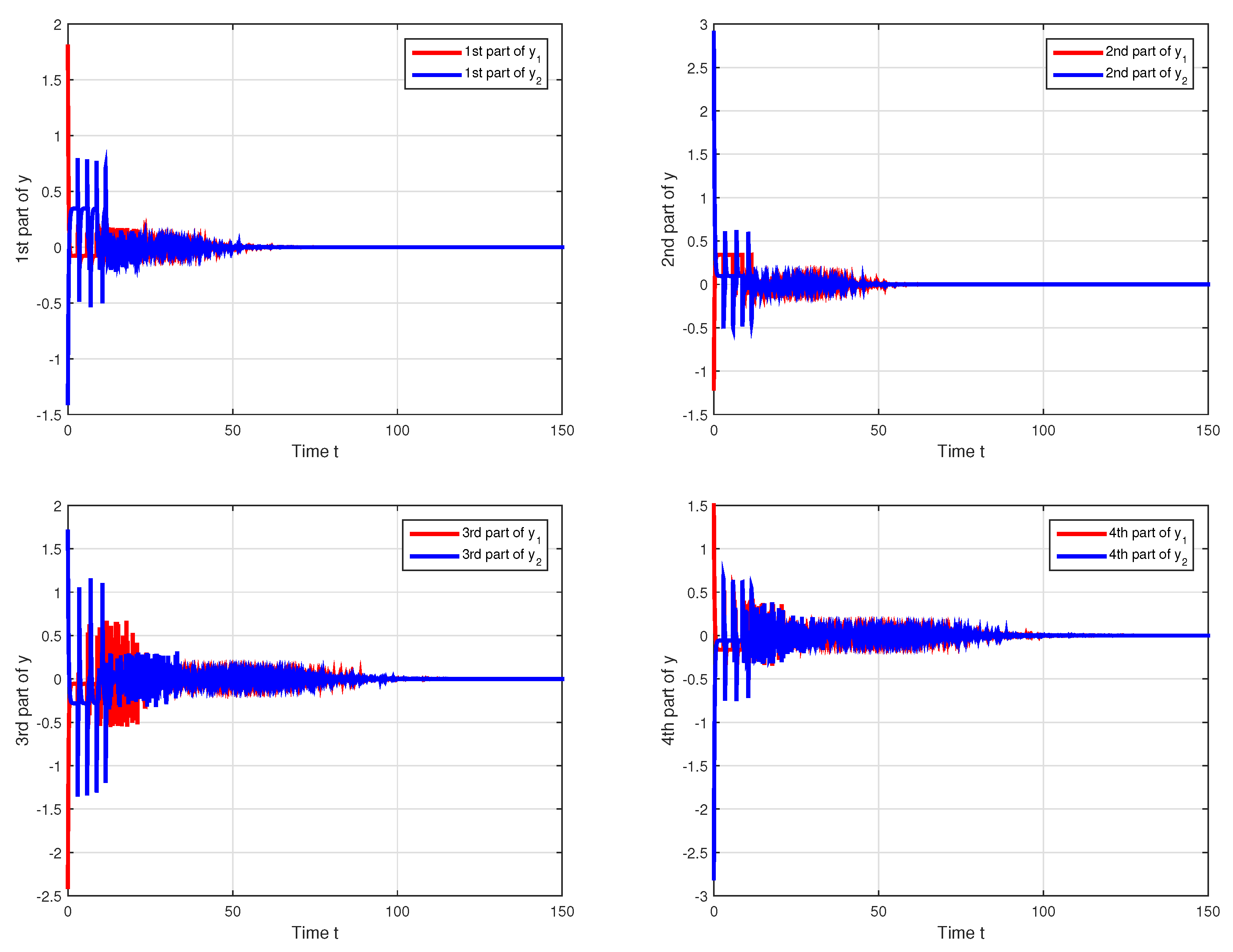
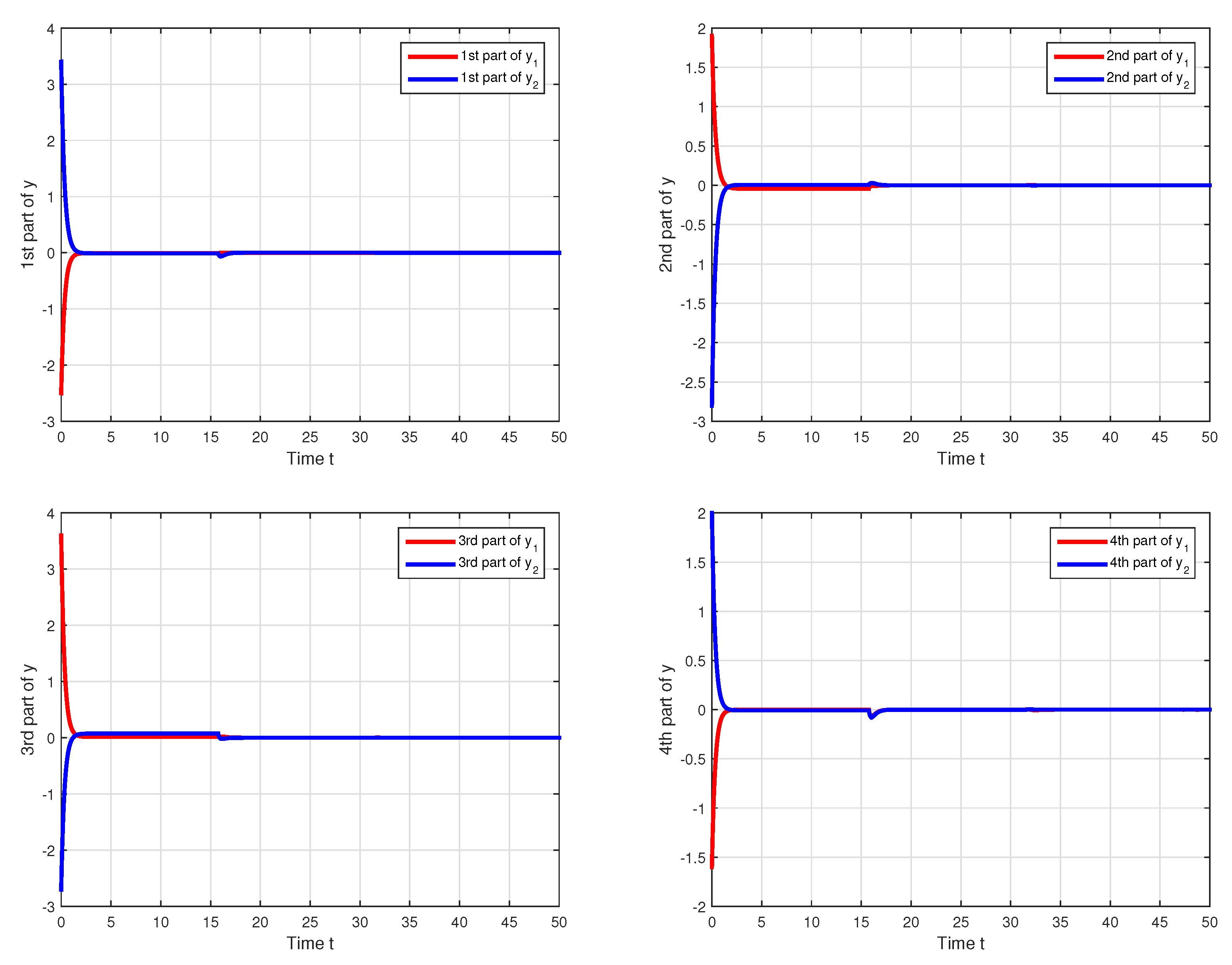
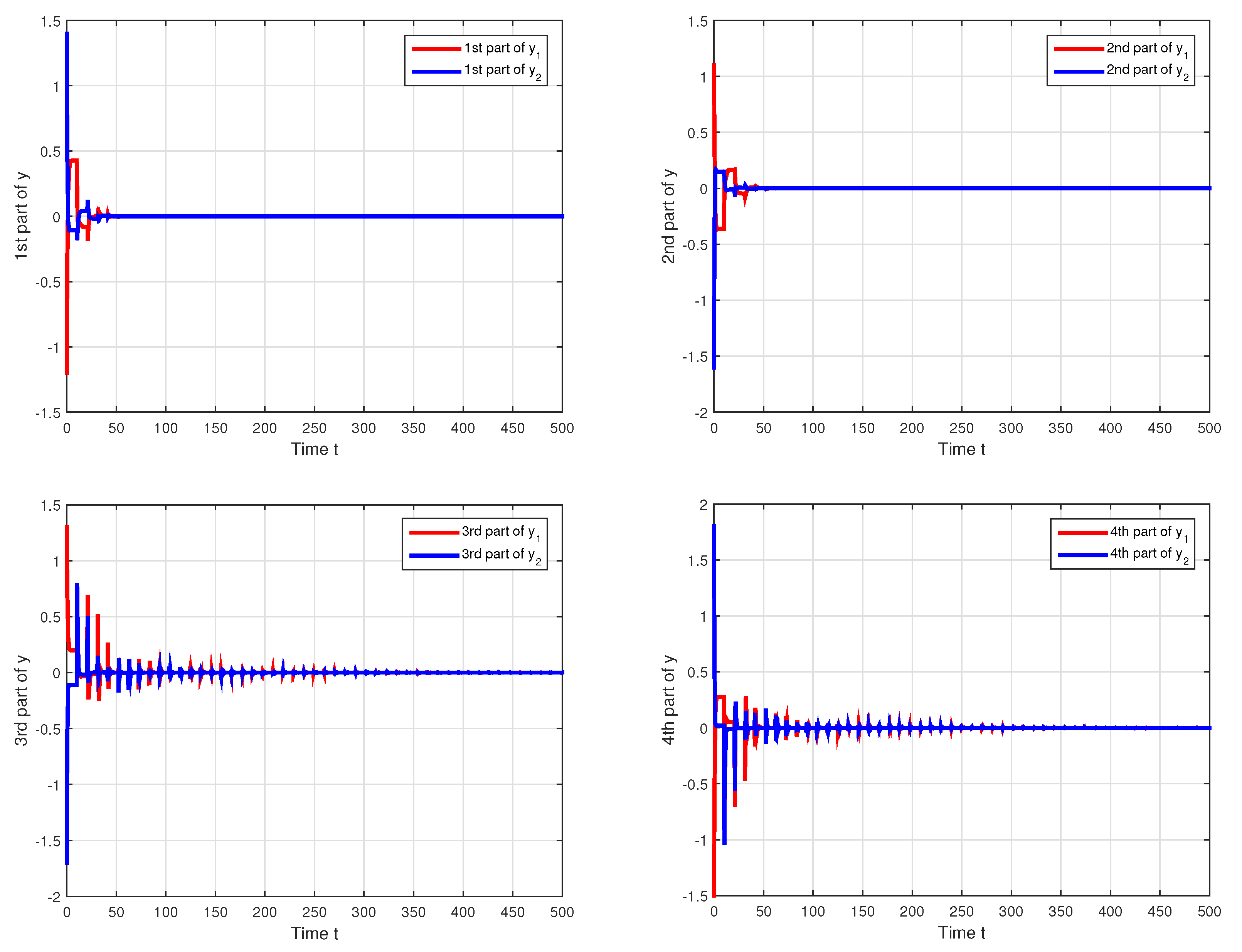
5. Numerical Example

In order to show the effectiveness and advantages of the proposed method, three interesting numerical examples are given as follows.

Example 1.

The delayed QVNTNN (Equation (1)) is rewritten as follows:

$$\dot{y}\left(t\right)-\mathcal{C}\dot{y}(t-\nu \left(t\right))=-\mathcal{D}y\left(t\right)+\mathcal{A}p\left(y\left(t\right)\right)+\mathcal{B}p\left(y(t-\nu \left(t\right))\right)+\kappa .$$

where $y=y_{11}+\mathrm{i}{y}_{12}+\mathrm{j}{y}_{21}+\mathrm{k}{y}_{22}\in {\mathfrak{Q}}^{2\times 1}$, and

$$\mathcal{A}=\left(\begin{array}{cc}0.2+0.5\mathrm{i}-0.5\mathrm{j}+0.1\mathrm{k}& 0.4+0.4\mathrm{i}-0.6\mathrm{j}+0.1\mathrm{k}\\ -0.5+0.2\mathrm{i}-0.1\mathrm{j}+0.5\mathrm{k}& 0.3+0.4\mathrm{i}+0.1\mathrm{j}+0.6\mathrm{k}\end{array}\right)$$

$$=\left(\begin{array}{cc}0.2+0.5\mathrm{i}& 0.4+0.4\mathrm{i}\\ -0.5+0.2\mathrm{i}& 0.3+0.4\mathrm{i}\end{array}\right)+\left(\begin{array}{cc}-0.5+0.1\mathrm{i}& -0.6+0.1\mathrm{i}\\ -0.1+0.5\mathrm{i}& 0.1+0.6\mathrm{i}\end{array}\right)\mathrm{j}$$

$$={\mathcal{A}}_1+{\mathcal{A}}_2\mathrm{j},$$

$$\mathcal{B}=\left(\begin{array}{cc}-0.3+0.4\mathrm{i}-0.5\mathrm{j}+0.2\mathrm{k}& 0.6-0.2\mathrm{i}-0.3\mathrm{j}-0.5\mathrm{k}\\ 0.2+0.8\mathrm{i}+0.2\mathrm{j}+0.5\mathrm{k}& -0.4-0.3\mathrm{i}-0.5\mathrm{j}-0.3\mathrm{k}\end{array}\right)$$

$$=\left(\begin{array}{cc}-0.3+0.4\mathrm{i}& 0.6-0.2\mathrm{i}\\ 0.2+0.8\mathrm{i}& -0.4-0.3\mathrm{i}\end{array}\right)+\left(\begin{array}{cc}-0.5+0.2\mathrm{i}& -0.3-0.5\mathrm{i}\\ 0.2+0.5\mathrm{i}& -0.5-0.3\mathrm{i}\end{array}\right)\mathrm{j}$$

$$={\mathcal{B}}_1+{\mathcal{B}}_2\mathrm{j},$$

$$\mathcal{C}=\left(\begin{array}{cc}0.1+0.05\mathrm{i}+0.2\mathrm{j}+0.05\mathrm{k}& 0.2+0.04\mathrm{i}+0.4\mathrm{j}+0.04\mathrm{k}\\ -0.1+0.04\mathrm{i}-0.5\mathrm{j}+0.02\mathrm{k}& 0.2+0.04\mathrm{i}+0.03\mathrm{j}+0.04\mathrm{k}\end{array}\right)$$

$$=\left(\begin{array}{cc}0.1+0.05\mathrm{i}& 0.2+0.04\mathrm{i}\\ -0.1+0.04\mathrm{i}& 0.2+0.04\mathrm{i}\end{array}\right)+\left(\begin{array}{cc}0.2+0.05\mathrm{i}& 0.4+0.04\mathrm{i}\\ -0.5+0.02\mathrm{i}& 0.03+0.04\mathrm{i}\end{array}\right)\mathrm{j}$$

$$={\mathcal{C}}_1+{\mathcal{C}}_2\mathrm{j},$$

$$\mathcal{D}=\left(\begin{array}{cc}5& 0\\ 0& 5\end{array}\right),\kappa ={(0,0)}^{*}.$$

In this example, we take the activation functions as $p\left(u\right)=0.5\left(\right|u+1|-|u-1\left|\right)+0.5\left(\right|u+1|-|u-1\left|\right)j$. Clearly, it can be confirmed that Assumption 2 satisfies ${\Lambda }_i=diag(0.01,0.01)(i=1,2,\dots ,8)$. Assume the time-varying delay satisfies $\nu \left(t\right)=12.1566\left|sin\right(t\left)\right|$; then, obviously, it can be computed that $\varsigma =0.5$, $\nu =12.1566$. In addition, let $\varpi =0.1$. It is easy to calculated that ${\beta }_1=0.1$, ${\beta }_2=e^{-0.05}$. By using the Yalmip toolbox to solve Corollary 1, we can obtain the following feasible solutions.

$$\mathcal{P}=\left(\begin{array}{cc}7.1417+0.0000\mathrm{i}& 1.0375+0.1874\mathrm{i}\\ 1.0375-0.1874\mathrm{i}& 6.9721+0.0000\mathrm{i}\end{array}\right)\times {10}^2,\mathcal{Q}=\left(\begin{array}{cc}2.9401+0.0000\mathrm{i}& 1.1097+0.2555\mathrm{i}\\ 1.1097-0.2555\mathrm{i}& 2.4352+0.0000\mathrm{i}\end{array}\right)\times {10}^3,$$

$$\mathcal{R}=\left(\begin{array}{cc}83.3051+0.0000\mathrm{i}& -18.2915+11.0733\mathrm{i}\\ -18.2915-11.0733\mathrm{i}& 82.7744+0.0000\mathrm{i}\end{array}\right),\mathcal{S}=\left(\begin{array}{cc}0.6318+0.0000\mathrm{i}& -0.0028+0.0653\mathrm{i}\\ -0.0028-0.0653\mathrm{i}& 0.6254+0.0000\mathrm{i}\end{array}\right),$$

$$\mathcal{W}=\left(\begin{array}{cc}51.2573+0.0000\mathrm{i}& 15.4123-1.1918\mathrm{i}\\ 15.4123+1.1918\mathrm{i}& 53.7044+0.0000\mathrm{i}\end{array}\right),{\mathcal{N}}_1=\left(\begin{array}{cc}1.2019& 0\\ 0& 1.2376\end{array}\right)\times {10}^3,$$

$${\mathcal{N}}_2=\left(\begin{array}{cc}923.8130& 0\\ 0& 866.7363\end{array}\right),{\mathcal{N}}_3=\left(\begin{array}{cc}462.6568& 0\\ 0& 479.7606\end{array}\right),{\mathcal{N}}_4=\left(\begin{array}{cc}1.1404& 0\\ 0& 1.0782\end{array}\right)\times {10}^3,$$

$${\mathcal{N}}_5=\left(\begin{array}{cc}1.1850+0.2537\mathrm{i}& 0.2186+0.3304\mathrm{i}\\ 0.1780+0.2630\mathrm{i}& 1.2111+0.2945\mathrm{i}\end{array}\right)\times {10}^2,{\mathcal{N}}_6=\left(\begin{array}{cc}3.7716+1.1880\mathrm{i}& 0.7546+1.5896\mathrm{i}\\ 1.0880+1.2376\mathrm{i}& 3.0510+1.4867\mathrm{i}\end{array}\right)\times {10}^2,$$

$${\mathcal{U}}_1=\left(\begin{array}{cc}0.0273+0.0000\mathrm{i}& -0.0052+0.0019\mathrm{i}\\ -0.0052-0.0019\mathrm{i}& 0.0200+0.0000\mathrm{i}\end{array}\right),{\mathcal{U}}_2=\left(\begin{array}{cc}0.7157+0.0000\mathrm{i}& 0.1415+0.1018\mathrm{i}\\ 0.1415-0.1018\mathrm{i}& 0.6476+0.0000\mathrm{i}\end{array}\right)\times {10}^3,$$

$${\mathcal{U}}_4=\left(\begin{array}{cc}-0.0131+0.0000\mathrm{i}& -0.0035-0.0007\mathrm{i}\\ -0.0035+0.0007\mathrm{i}& -0.0124+0.0000\mathrm{i}\end{array}\right),{\mathcal{U}}_5=\left(\begin{array}{cc}0.0264+0.0000\mathrm{i}& -0.0050+0.0019\mathrm{i}\\ -0.0050-0.0019\mathrm{i}& 0.0192+0.0000\mathrm{i}\end{array}\right),$$

$${\mathcal{U}}_6=\left(\begin{array}{cc}0.0012+0.0000\mathrm{i}& -0.0003+0.0002\mathrm{i}\\ -0.0003-0.0002\mathrm{i}& 0.0009+0.0000\mathrm{i}\end{array}\right),{\mathcal{U}}_8=\left(\begin{array}{cc}0.0024+0.0000\mathrm{i}& -0.0210-0.0019\mathrm{i}\\ -0.0210+0.0019\mathrm{i}& -0.0049+0.0000\mathrm{i}\end{array}\right),$$

$$\mathcal{X}=\left(\begin{array}{cc}-6.0218+0.0000\mathrm{i}& -4.6899-1.0333\mathrm{i}\\ -4.6899+1.0333\mathrm{i}& -3.9657+0.0000\mathrm{i}\end{array}\right)\times {10}^2,\mathcal{Y}=\left(\begin{array}{cc}1.4287+0.0000\mathrm{i}& -0.2653+0.1715\mathrm{i}\\ -0.2653-0.1715\mathrm{i}& 1.4202+0.0000\mathrm{i}\end{array}\right)\times {10}^2.$$

Thus, the equilibrium point of QVNTNNs (Equation (1)) is globally exponentially stable. Figure 1 shows four parts of the state responses of the QVNTNNs (Equation (1)).

Example 2.

The delayed QVNTNN (Equation (1)) is rewritten as follows

$$\dot{y}\left(t\right)-\mathcal{C}\dot{y}(t-\nu \left(t\right))=-\mathcal{D}y\left(t\right)+\mathcal{A}p\left(y\left(t\right)\right)+\mathcal{B}p\left(y(t-\nu \left(t\right))\right)+\kappa .$$

where $y=y_{11}+\mathrm{i}{y}_{12}+\mathrm{j}{y}_{21}+\mathrm{k}{y}_{22}\in {\mathfrak{Q}}^{2\times 1}$, and

$$\mathcal{A}=\left(\begin{array}{cc}0.4+0.3\mathrm{i}-0.5\mathrm{j}+0.4\mathrm{k}& -0.7+0.7\mathrm{i}-0.6\mathrm{j}+0.14\mathrm{k}\\ -0.6-0.4\mathrm{i}+0.14\mathrm{j}+0.53\mathrm{k}& 0.7+0.3\mathrm{i}+0.1\mathrm{j}+0.6\mathrm{k}\end{array}\right)$$

$$=\left(\begin{array}{cc}0.4+0.3\mathrm{i}& -0.7+0.7\mathrm{i}\\ -0.6-0.4\mathrm{i}& 0.7+0.3\mathrm{i}\end{array}\right)+\left(\begin{array}{cc}-0.5+0.4\mathrm{i}& -0.6+0.14\mathrm{i}\\ 0.14+0.53\mathrm{i}& 0.1+0.6\mathrm{i}\end{array}\right)\mathrm{j}$$

$$={\mathcal{A}}_1+{\mathcal{A}}_2\mathrm{j},$$

$$\mathcal{B}=\left(\begin{array}{cc}0.7\mathrm{j}+0.1\mathrm{k}& 0.5-0.3\mathrm{i}+0.6\mathrm{j}-0.1\mathrm{k}\\ 0.7\mathrm{i}+0.2\mathrm{j}+0.6\mathrm{k}& -0.1+0.6\mathrm{i}-0.3\mathrm{j}-0.3\mathrm{k}\end{array}\right)$$

$$=\left(\begin{array}{cc}0& 0.5-0.3\mathrm{i}\\ 0.7\mathrm{i}& -0.1+0.6\mathrm{i}\end{array}\right)+\left(\begin{array}{cc}0.7+0.1\mathrm{i}& 0.6-0.1\mathrm{i}\\ 0.2+0.6\mathrm{i}& -0.3-0.3\mathrm{i}\end{array}\right)\mathrm{j}$$

$$={\mathcal{B}}_1+{\mathcal{B}}_2\mathrm{j},$$

$$\mathcal{C}=\left(\begin{array}{cc}0.07+0.05\mathrm{i}-0.06\mathrm{j}+0.03\mathrm{k}& 0.06+0.02\mathrm{i}-0.04\mathrm{j}-0.02\mathrm{k}\\ 0.04+0.04\mathrm{i}+0.01\mathrm{j}+0.04\mathrm{k}& 0.06+0.04\mathrm{i}-0.02\mathrm{j}-0.03\mathrm{k}\end{array}\right)$$

$$=\left(\begin{array}{cc}0.07+0.05\mathrm{i}& 0.06+0.02\mathrm{i}\\ 0.04+0.04\mathrm{i}& 0.06+0.04\mathrm{i}\end{array}\right)+\left(\begin{array}{cc}-0.06+0.03\mathrm{i}& -0.04-0.02\mathrm{i}\\ 0.01+0.04\mathrm{i}& -0.02-0.03\mathrm{i}\end{array}\right)\mathrm{j}$$

$$={\mathcal{C}}_1+{\mathcal{C}}_2\mathrm{j},$$

$$\mathcal{D}=\left(\begin{array}{cc}3& 0\\ 0& 3\end{array}\right),\kappa ={(0,0)}^{*}.$$

Here, we use $p\left(u\right)=\frac{1}{25}\left(\right|u+1|-|u-1\left|\right)+\frac{1}{10}\left(\right|u+1|-|u-1\left|\right)\mathrm{j}$ as the activation function. Clearly, it can be confirmed that Assumption 2 satisfies ${\Lambda }_1={\Lambda }_3={\Lambda }_5={\Lambda }_7=diag(0.08,0.08)$, ${\Lambda }_2={\Lambda }_4={\Lambda }_6={\Lambda }_8=diag(0.2,0.2)$. Assuming that the time-varying delay satisfies $\nu \left(t\right)=1+15.7508sin\left(t\right)$, it can be obviously computed that $\varsigma =0.2$, $\nu =15.7506$. In addition, let $\varpi =0.1$; then, it is easy to calculate that ${\beta }_1=\frac{1}{20\nu }$, ${\beta }_2={0.2}^{0.1}$. Using the Yalmip toolbox, Corollary 2 can be solved. After calculation, a feasible solution is obtained.

$$\mathcal{P}=\left(\begin{array}{cc}8.1305+0.0000\mathrm{i}& 1.6705-1.3097\mathrm{i}\\ 1.6705+1.3097\mathrm{i}& 7.0427+0.0000\mathrm{i}\end{array}\right)\times {10}^2,\mathcal{Q}=\left(\begin{array}{cc}1.7466+0.0000\mathrm{i}& 0.6000-0.3775\mathrm{i}\\ 0.6000+0.3775\mathrm{i}& 1.6290+0.0000\mathrm{i}\end{array}\right)\times {10}^3,$$

$$\mathcal{R}=\left(\begin{array}{cc}1.3109+0.0000\mathrm{i}& 0.2807-0.2632\mathrm{i}\\ 0.2807+0.2632\mathrm{i}& 1.3281+0.0000\mathrm{i}\end{array}\right)\times {10}^2,\mathcal{S}=\left(\begin{array}{cc}0.7719+0.0000\mathrm{i}& 0.1719-0.1559\mathrm{i}\\ 0.1719+0.1559\mathrm{i}& 0.6759+0.0000\mathrm{i}\end{array}\right),$$

$$\mathcal{W}=\left(\begin{array}{cc}74.2120+0.0000\mathrm{i}& 23.1226-14.6231\mathrm{i}\\ 23.1226+14.6231\mathrm{i}& 63.5486+0.0000\mathrm{i}\end{array}\right),{\mathcal{N}}_1=\left(\begin{array}{cc}1.5729& 0\\ 0& 1.4706\end{array}\right)\times {10}^3,$$

$${\mathcal{N}}_2=\left(\begin{array}{cc}1.3224& 0\\ 0& 1.2860\end{array}\right)\times {10}^3,{\mathcal{N}}_3=\left(\begin{array}{cc}1.0368& 0\\ 0& 1.0848\end{array}\right)\times {10}^3,{\mathcal{N}}_4=\left(\begin{array}{cc}1.2418& 0\\ 0& 1.1836\end{array}\right)\times {10}^3,$$

$${\mathcal{N}}_5=\left(\begin{array}{cc}2.4691+0.6137\mathrm{i}& 0.3724+0.2442\mathrm{i}\\ 0.2087+0.6044\mathrm{i}& 2.1374+0.3713\mathrm{i}\end{array}\right)\times {10}^2,{\mathcal{N}}_6=\left(\begin{array}{cc}5.1458+1.1580\mathrm{i}& 0.5341+0.9446\mathrm{i}\\ 0.5025+1.4435\mathrm{i}& 4.6514+1.0152\mathrm{i}\end{array}\right)\times {10}^2,$$

$${\mathcal{U}}_1=\left(\begin{array}{cc}-0.0232+0.0000\mathrm{i}& -0.0684+0.0823\mathrm{i}\\ -0.0684-0.0823\mathrm{i}& 0.0371+0.0000\mathrm{i}\end{array}\right),{\mathcal{U}}_2=\left(\begin{array}{cc}0.0050+0.0000\mathrm{i}& 0.0029-0.0023\mathrm{i}\\ 0.0029+0.0023\mathrm{i}& 0.0037+0.0000\mathrm{i}\end{array}\right),$$

$${\mathcal{U}}_4=\left(\begin{array}{cc}-0.0518+0.0000\mathrm{i}& -0.0300+0.0223\mathrm{i}\\ -0.0300-0.0223\mathrm{i}& -0.0392+0.0000\mathrm{i}\end{array}\right),{\mathcal{U}}_5=\left(\begin{array}{cc}-0.0228+0.0000\mathrm{i}& -0.0500+0.0575\mathrm{i}\\ -0.0500-0.0575\mathrm{i}& 0.0186+0.0000\mathrm{i}\end{array}\right),$$

$${\mathcal{U}}_6=\left(\begin{array}{cc}0.6729+0.0000\mathrm{i}& 0.0180-0.0231\mathrm{i}\\ 0.0180+0.0231\mathrm{i}& 0.6275+0.0000\mathrm{i}\end{array}\right)\times {10}^3,{\mathcal{U}}_8=\left(\begin{array}{cc}-0.0658+0.0000\mathrm{i}& -0.0529+0.0383\mathrm{i}\\ -0.0529-0.0383\mathrm{i}& -0.0454+0.0000\mathrm{i}\end{array}\right),$$

$$\mathcal{X}=\left(\begin{array}{cc}-2.1273+0.0000\mathrm{i}& -2.7733+1.6689\mathrm{i}\\ -2.7733-1.6689\mathrm{i}& -1.9530+0.0000\mathrm{i}\end{array}\right)\times {10}^2,\mathcal{Y}=\left(\begin{array}{cc}3.2197+0.0000\mathrm{i}& 0.4433-0.6310\mathrm{i}\\ 0.4433+0.6310\mathrm{i}& 3.2625+0.0000\mathrm{i}\end{array}\right)\times {10}^2.$$

Thus, the equilibrium point of QVNTNNs (Equation (1)) is globally power-stable. Figure 2 shows four parts of the state responses of the QVNTNNs (Equation (1)).

We have listed the maximal allowable bounds of $\nu$ for QVNNs and QVNTNNs in

Table 1. The maximal allowable bounds of $\nu$.

Condition	$\mathit{QVNN}$	QVNTNN
global exponential stability	$13.9447$	$12.1566$
global power-stability	$15.7909$	$15.7508$
global log-stability	$15.0446$	$10.3423$

. From the comparison of QVNNs and QVNTNNs, we can see that the maximal delay bounds are bigger than those of QVNTNNs.

Example 3.

The delayed QVNTNN (Equation (1)) is rewritten as follows:

$$\dot{y}\left(t\right)-\mathcal{C}\dot{y}(t-\nu \left(t\right))=-\mathcal{D}y\left(t\right)+\mathcal{A}p\left(y\left(t\right)\right)+\mathcal{B}p\left(y(t-\nu \left(t\right))\right)+\kappa .$$

where $y=y_{11}+\mathrm{i}{y}_{12}+\mathrm{j}{y}_{21}+\mathrm{k}{y}_{22}\in {\mathfrak{Q}}^{2\times 1}$, and

$$\mathcal{A}=\left(\begin{array}{cc}0.7+1\mathrm{i}-0.2\mathrm{j}+0.4\mathrm{k}& 0.3+1.2\mathrm{i}-0.4\mathrm{j}+0.3\mathrm{k}\\ 0.3-0.2\mathrm{i}+0.2\mathrm{j}+0.1\mathrm{k}& 1+\mathrm{i}-0.2\mathrm{j}+0.4\mathrm{k}\end{array}\right)$$

$$=\left(\begin{array}{cc}0.7+1\mathrm{i}& 0.3+1.2\mathrm{i}\\ 0.3-0.2\mathrm{i}& 1+1\mathrm{i}\end{array}\right)+\left(\begin{array}{cc}-0.2+0.4\mathrm{i}& -0.4+0.3\mathrm{i}\\ 0.2+0.1\mathrm{i}& -0.2+0.4\mathrm{i}\end{array}\right)\mathrm{j}$$

$$={\mathcal{A}}_1+{\mathcal{A}}_2\mathrm{j},$$

$$\mathcal{B}=\left(\begin{array}{cc}-0.4+0.7\mathrm{i}+0.2\mathrm{j}+0.5\mathrm{k}& 1+0.5\mathrm{i}+0.3\mathrm{j}-0.5\mathrm{k}\\ 0.3+0.2\mathrm{i}-0.2\mathrm{j}+0.1\mathrm{k}& -0.5+0.5\mathrm{i}+0.2\mathrm{j}+0.4\mathrm{k}\end{array}\right)$$

$$=\left(\begin{array}{cc}-0.4+0.7\mathrm{i}& 1+0.5\mathrm{i}\\ 0.3+0.2\mathrm{i}& -0.5+0.5\mathrm{i}\end{array}\right)+\left(\begin{array}{cc}0.2+0.5\mathrm{i}& 0.3-0.5\mathrm{i}\\ -0.2+0.1\mathrm{i}& 0.2+0.4\mathrm{i}\end{array}\right)\mathrm{j}$$

$$={\mathcal{B}}_1+{\mathcal{B}}_2\mathrm{j},$$

$$\mathcal{C}=\left(\begin{array}{cc}0.2+0.08\mathrm{i}+0.3\mathrm{j}+0.05\mathrm{k}& 0.5+0.08\mathrm{i}+0.8\mathrm{j}+0.01\mathrm{k}\\ -0.3-0.02\mathrm{i}-0.5\mathrm{j}+0.02\mathrm{k}& -0.2+0.04\mathrm{i}+1\mathrm{j}+0.02\mathrm{k}\end{array}\right)$$

$$=\left(\begin{array}{cc}0.2+0.08\mathrm{i}& 0.5+0.08\mathrm{i}\\ -0.3-0.02\mathrm{i}& -0.2+0.04\mathrm{i}\end{array}\right)+\left(\begin{array}{cc}0.3+0.05\mathrm{i}& 0.8+0.01\mathrm{i}\\ -0.5+0.02\mathrm{i}& 1+0.02\mathrm{i}\end{array}\right)\mathrm{j}$$

$$={\mathcal{C}}_1+{\mathcal{C}}_2\mathrm{j},$$

$$\mathcal{D}=\left(\begin{array}{cc}1.8& 0\\ 0& 2.8\end{array}\right),\kappa ={(0,0)}^{*}.$$

For this example, the activation function is chosen as $p\left(u\right)=0.5tanh\left(u\right)+0.5tanh\left(u\right)\mathrm{j}$. Clearly, it can be verified that Assumption 2 is satisfied with ${\Lambda }_1={\Lambda }_3={\Lambda }_5={\Lambda }_7=diag(0.07,0.07)$, ${\Lambda }_2={\Lambda }_4={\Lambda }_6={\Lambda }_8=diag(0.3,0.3)$. Assuming that the time-varying delay satisfies $\nu \left(t\right)=10.3423\left|sin\right(t\left)\right|$, it can be obviously computed that $\varsigma =0.5$, $\nu =10.3423$. In addition, let $\varpi =0.1$; then, it is easy to calculate that ${\beta }_1=\frac{1}{10e}$, ${\beta }_2=\frac{1}{ln(e+0.1\nu )}$. By using the Yalmip toolbox, Corollary 3 can be solved. The following feasible solutions were calculated by us:

$$\mathcal{P}=\left(\begin{array}{cc}3.6113+0.0000\mathrm{i}& -0.1457-0.3895\mathrm{i}\\ -0.1457+0.3895\mathrm{i}& 2.2912+0.0000\mathrm{i}\end{array}\right)\times {10}^2,\mathcal{Q}=\left(\begin{array}{cc}1.0170+0.0000\mathrm{i}& -0.1735-0.1745\mathrm{i}\\ -0.1735+0.1745\mathrm{i}& 1.3937+0.0000\mathrm{i}\end{array}\right)\times {10}^2,$$

$$\mathcal{R}=\left(\begin{array}{cc}1.5034+0.0000\mathrm{i}& -0.6070-0.4689\mathrm{i}\\ -0.6070+0.4689\mathrm{i}& 1.0799+0.0000\mathrm{i}\end{array}\right)\times {10}^2,\mathcal{S}=\left(\begin{array}{cc}1.3172+0.0000\mathrm{i}& -0.0604-0.1931\mathrm{i}\\ -0.0604+0.1931\mathrm{i}& 0.5848+0.0000\mathrm{i}\end{array}\right),$$

$$\mathcal{W}=\left(\begin{array}{cc}41.0682+0.0000\mathrm{i}& -1.8619-5.9645\mathrm{i}\\ -1.8619+5.9645\mathrm{i}& 18.7619+0.0000\mathrm{i}\end{array}\right),{\mathcal{N}}_1=\left(\begin{array}{cc}780.2274& 0\\ 0& 619.7779\end{array}\right),$$

$${\mathcal{N}}_2=\left(\begin{array}{cc}663.6841& 0\\ 0& 381.4323\end{array}\right),{\mathcal{N}}_3=\left(\begin{array}{cc}1.0702& 0\\ 0& 0.6026\end{array}\right)\times {10}^3,{\mathcal{N}}_4=\left(\begin{array}{cc}629.9553& 0\\ 0& 528.2100\end{array}\right),$$

$${\mathcal{N}}_5=\left(\begin{array}{cc}1.8379+0.2680\mathrm{i}& 0.0879+0.1924\mathrm{i}\\ 0.1497+0.1378\mathrm{i}& 0.7496+0.1278\mathrm{i}\end{array}\right)\times {10}^2,{\mathcal{N}}_6=\left(\begin{array}{cc}3.6887+0.4126\mathrm{i}& 0.1864+0.5835\mathrm{i}\\ 0.2439+0.1794\mathrm{i}& 1.4943+0.2445\mathrm{i}\end{array}\right)\times {10}^2,$$

$${\mathcal{U}}_1=\left(\begin{array}{cc}-0.1033+0.0000\mathrm{i}& -0.0089-0.0339\mathrm{i}\\ -0.0089+0.0339\mathrm{i}& -0.2079+0.0000\mathrm{i}\end{array}\right),{\mathcal{U}}_2=\left(\begin{array}{cc}0.0075+0.0000\mathrm{i}& 0.0005-0.0002\mathrm{i}\\ 0.0005+0.0002\mathrm{i}& 0.0018+0.0000\mathrm{i}\end{array}\right),$$

$${\mathcal{U}}_4=\left(\begin{array}{cc}-0.0712+0.0000\mathrm{i}& -0.0021+0.0060\mathrm{i}\\ -0.0021-0.0060\mathrm{i}& -0.0327+0.0000\mathrm{i}\end{array}\right),{\mathcal{U}}_5=\left(\begin{array}{cc}-0.0460+0.0000\mathrm{i}& -0.0147+0.0212\mathrm{i}\\ -0.0147-0.0212\mathrm{i}& 0.0285+0.0000\mathrm{i}\end{array}\right),$$

$${\mathcal{U}}_6=\left(\begin{array}{cc}0.0175+0.0000\mathrm{i}& 0.0005-0.0017\mathrm{i}\\ 0.0005+0.0017\mathrm{i}& 0.0026+0.0000\mathrm{i}\end{array}\right),{\mathcal{U}}_8=\left(\begin{array}{cc}0.0543+0.0000\mathrm{i}& -0.0027-0.0120\mathrm{i}\\ -0.0027+0.0120\mathrm{i}& -0.0099+0.0000\mathrm{i}\end{array}\right),$$

$$\mathcal{X}=\left(\begin{array}{cc}3.7674+0.0000\mathrm{i}& -0.0512-0.0312\mathrm{i}\\ -0.0512+0.0312\mathrm{i}& 2.8247+0.0000\mathrm{i}\end{array}\right)\times {10}^2,\mathcal{Y}=\left(\begin{array}{cc}1.7454+0.0000\mathrm{i}& -0.6159-0.3628\mathrm{i}\\ -0.6159+0.3628\mathrm{i}& 1.3755+0.0000\mathrm{i}\end{array}\right)\times {10}^2.$$

Thus, the equilibrium point of QVNTNNs (Equation (1)) is globally log-stable. Figure 3 shows four parts of the state responses of the QVNTNNs (Equation (1)).

6. Conclusions

In this paper, the global $\mu$-stability problem of QVNTNNs with time-varying delays is discussed. Firstly, the QVNTNNs are transformed into two complex-valued systems by using a transformation to reduce the complexity of the computation generated by the non-commutativity of quaternion multiplication. A new convex inequality in the complex field is introduced. Secondly, the conditions for the existence and uniqueness of the equilibrium point are obtained by primarily applying the homeomorphism theory. Thirdly, the global stability conditions of the complex-valued systems are provided by constructing a novel Lyapunov–Krasovskii functional, using an integral inequality technique, and reciprocal convex combination approach. The gained global $\mu$-stability conditions are divided into three different kinds of stability forms by varying the positive continuous function $\mu \left(t\right)$. In the end, three reliable examples and a simulation are provided to guarantee the validity of the obtained LMIs conditions. In the future, the problem of the stability, stochasticity, and synchronization of QVNTNNs with time delays and the QVNTNN with Markovian switching will be considered based on the results in this article.

References

1. Birx, D.L.; Pipenberg, S.J. A complex mapping network for phase sensitive classification. IEEE Trans. Neural Netw. 1993, 4, 127–135. [Google Scholar] [CrossRef] [PubMed]
2. Forster, B. Five Good Reasons for Complex-Valued Transforms in Image Processing; Springer International Publishing: Cham, Switzerland, 2014. [Google Scholar]
3. Arima, Y. Envelope-detection Millimeter-wave Active Imaging System using Complex-Valued Self-Organizing Map Image Processing. Water Resour. Res. 2015, 50, 1846. [Google Scholar]
4. Filliat, D.; Battesti, E.; Bazeille, S. RGBD object recognition and visual texture classification for indoor semantic mapping. In Proceedings of the IEEE International Conference on Technologies for Practical Robot Applications, Woburn, MA, USA, 23–24 April 2012. [Google Scholar]
5. Hirose, A.; Eckmiller, R. Behavior control of coherent-type neural networks by carrier-frequency modulation. IEEE Trans. Neural Netw. 1996, 7, 1032–1034. [Google Scholar] [CrossRef] [PubMed]
6. Xu, D.S.; Tan, M.C. Delay-independent stability criteria for complex-valued BAM neutral-type neural networks with time delays. Nonlinear Dyn. 2017, 89, 819–832. [Google Scholar] [CrossRef]
7. Guo, R.; Zhang, Z.; Liu, X.; Lin, C. Existence, uniqueness, and exponential stability analysis for complex-valued memristor-based BAM neural networks with time delays. Appl. Math. Comput. 2017, 311, 100–117. [Google Scholar] [CrossRef]
8. Liu, D.; Zhu, S.; Ye, E. Synchronization stability of memristor-based complex-valued neural networks with time delays. Neural Netw. 2017, 96, 115–127. [Google Scholar] [CrossRef] [PubMed]
9. Zhang, H.; Wang, X.Y. Complex projective synchronization of complex-valued neural network with structure identification. J. Frankl. Inst. 2017, 354, 5011–5025. [Google Scholar] [CrossRef]
10. Ali, M.S.; Yogambigai, J. Extended dissipative synchronization of complex dynamical networks with additive time-varying delay and discrete-time information. J. Comput. Appl. Math. 2019, 348, 28–341. [Google Scholar]
11. Zhang, L.; Yang, X.; Xu, C. Exponential synchronization of complex-valued complex networks with time-varying delays and stochastic perturbations via time-delayed impulsive control. Appl. Math. Comput. 2017, 306, 22–30. [Google Scholar] [CrossRef]
12. Wang, J.F.; Tian, L.X. Global Lagrange stability for inertial neural networks with mixed time-varying delays. Neurocomputing 2017, 235, 140–146. [Google Scholar] [CrossRef]
13. Tang, Q.; Jian, J.G. Matrix measure based exponential stabilization for complex-valued inertial neural networks with time-varying delays using impulsive control. Neurocomputing 2018, 273, 251–259. [Google Scholar] [CrossRef]
14. Li, X.F.; Fang, J.A.; Li, H.Y. Master-slave exponential synchronization of delayed complex-valued memristor-based neural networks via impulsive control. Neural Netw. 2017, 93, 165–175. [Google Scholar] [CrossRef] [PubMed]
15. Song, Q.K.; Zhao, Z.J.; Liu, Y.R. Impulsive effects on stability of discrete-time complex-valued neural networks with both discrete and distributed time-varying delays. Neurocomputing 2015, 168, 1044–1050. [Google Scholar] [CrossRef]
16. Jian, J.G.; Wan, P. Global exponential convergence of fuzzy complex-valued neural networks with time-varying delays and impulsive effects. Fuzzy Sets Syst. 2018, 338, 23–39. [Google Scholar] [CrossRef]
17. Huang, C.D.; Cao, J.D.; Xiao, M.; Alsaedi, A.; Haya, T. Bifurcations in a delayed fractional complex-valued neural network. Appl. Math. Comput. 2017, 292, 210–227. [Google Scholar] [CrossRef]
18. Miron, S.; Le Bihan, N.; Mars, J.I. Quaternion-music for vector-sensor array processing. IEEE Trans. Signal Process. 2006, 54, 1218–1229. [Google Scholar] [CrossRef]
19. Ell, T.; Sangwine, S.J. Hypercomplex fourier transforms of color images. IEEE Trans. Image Process. 2007, 16, 22–35. [Google Scholar] [CrossRef]
20. Took, C.C.; Strbac, G.; Aihara, K.; Mandic, D.P. Quaternion-valued short-term joint forecasting of three-dimensional wind and atmospheric parameters. Renew. Energy 2011, 36, 1754–1760. [Google Scholar] [CrossRef]
21. Isokawa, T.; Kusakabe, T.; Matsui, N.; Peper, F. Quaternion Neural Network and It’s Application. In Knowledge-Based Intelligent Information and Engineering Systems; Springer: Berlin/Heidelberg, Germany, 2003; pp. 318–324. [Google Scholar]
22. Mandic, D.P.; Jahanchahi, C.; Took, C.C. A quaternion gradient operator and it is applications. IEEE Trans. Signal Process. Lett. 2011, 18, 47–50. [Google Scholar] [CrossRef]
23. Sudbery, A. Quaternionic analysis. Math. Proc. Camb. Philos. Soc. 1979, 85, 199–225. [Google Scholar] [CrossRef]
24. Bihan, N.L.; Sangwine, S.J. Quaternion principal component analysis of color images. In Proceeding of the IEEE International Conference on Image Processing, Barcelona, Spain, 14–17 September 2003. [Google Scholar]
25. Mandic, D.P.; Goh, V.S.L. Complex Valued Nonlinear Adaptive Filters: Noncircularity; Widely Linear and Neural Models; Wiley Publishing: Hoboken, NJ, USA, 2009. [Google Scholar]
26. Liu, Y.; Zhang, D.D.; Lu, J.Q. Global μ-stability criteria for quaternion-valued neural networks with unbounded time-varying delays. Inf. Sci. 2016, 360, 273–288. [Google Scholar] [CrossRef]
27. Chen, X.; Li, Z.; Song, Q. Robust stability analysis of quaternion-valued neural networks with time delays and parameter uncertainties. Neural Netw. 2017, 91, 55–65. [Google Scholar] [CrossRef] [PubMed]
28. Li, Y.; Li, B.; Yao, S. The global exponential pseudo almost periodic synchronization of quaternion-valued cellular neural networks with time-varying delays. Neurocomputing 2018, 303, 75–87. [Google Scholar] [CrossRef]
29. Liu, Y.; Zhang, D.D.; Lou, J.Q.; Cao, J.D. Stability analysis of quaternion-valued neural networks: decomposition and direct approaches. IEEE Trans. Neural Netw. Learn. Syst. 2018, 29, 4201–4211. [Google Scholar] [PubMed]
30. Ali, M.S.; Saravanakumar, R.; Cao, J. New passivity criteria for memristor-based neutral-type stochastic BAM neural networks with mixed time-varying delays. Neurocomputing 2016, 171, 1533–1547. [Google Scholar]
31. Zhou, H.; Zhou, Z.; Jiang, W. Almost periodic solutions for neutral type BAM neural networks with distributed leakage delays on time scales. Neurocomputing 2015, 157, 223–230. [Google Scholar] [CrossRef]
32. Lakshmanan, S.; Lim, C.P.; Prakash, M.; Nahavandi, S.; Balasubramaniam, P. Neutral-type of delayed inertial neural networks and their stability analysis using the LMI Approach. Neurocomputing 2016, 230, 243–250. [Google Scholar] [CrossRef]
33. Wang, Y.; Zhang, X.; Zhang, X. Neutral-delay-range-dependent absolute stability criteria for neutral-type Lur’e systems with time-varying delays. J. Frankl. Inst. 2016, 353, 5025–5039. [Google Scholar] [CrossRef]
34. Wu, T.; Xiong, L.L.; Cao, J.D.; Liu, Z.X.; Zhang, H.Y. New stability and stabilization conditions for stochastic neural networks of neutral type with Markovian jumping parameters. J. Frankl. Inst. 2018, 355, 8462–8483. [Google Scholar] [CrossRef]
35. Xiong, L.L.; Zhang, H.Y.; Li, Y.K.; Liu, Z.X. Improved stability and H∞ performance for neutral systems with uncertain Markovian jump. Nonlinear Anal. Hybrid Syst. 2016, 19, 13–25. [Google Scholar] [CrossRef]
36. Xiong, L.L.; Tian, J.K.; Liu, X.Z. Stability analysis for neutral Markovian jump systems with partially unknown transition probabilities. J. Frankl. Inst. 2012, 349, 2193–2214. [Google Scholar] [CrossRef]
37. Wu, T.; Cao, J.D.; Xiong, L.L.; Ahmad, B. Exponential passivity conditions on neutral stochastic neural networks with leakage delay and partially unknown transition probabilities in Markovian jump. Adv. Differ. Eq. 2018, 2018, 317. [Google Scholar] [CrossRef]
38. Xiong, L.L.; Cheng, J.; Liu, X.Z.; Wu, T. Improved conditions for neutral delay systems with novel inequalities. J. Nonlinear Sci. Appl. 2017, 10, 2309–2317. [Google Scholar] [CrossRef] [Green Version]
39. Ghadiri, H.; Motlagh, M.R.J.; Yazdi, M.B. Robust stabilization for uncertain switched neutral systems with interval time-varying mixed delays. Nonlinear Anal. Hybrid Syst. 2014, 13, 2–21. [Google Scholar] [CrossRef]
40. Salamon, D. Control and Observation of Neutral Systems; Pitman Advanced Publishing Program: Boston, MA, USA, 1984. [Google Scholar]
41. Xiong, W.J.; Liang, J.L. Novel stability criteria for neutral systems with multiple time-delays. Chaos Solitons Fractals 2007, 32, 1735–1741. [Google Scholar] [CrossRef]
42. Xu, S.; Lam, J.; Ho, D.W.C.; Zou, Y. Delay-dependent exponential stability for a class of neural networks with time delays. J. Comput. Appl. Math. 2005, 183, 16–28. [Google Scholar] [CrossRef] [Green Version]
43. Zuo, Z.Q.; Wang, Y. Novel Delay-Dependent Exponential Stability Analysis for a Class of Delayed Neural Networks. In Proceedings of the International Conference on Intelligent Computing, Kunming, China, 16–19 August 2006; pp. 216–226. [Google Scholar]
44. Hale, J.K. The Theory of Functional Differential Equations; Applied Mathematical Sciences; Springer-Verlag: New York, NY, USA, 1977. [Google Scholar]
45. Velmurugan, G.; Rakkiyappan, R.; Cao, J. Further analysis of global μ-stability of complex-valued neural networks with unbounded time-varying delays. Neural Netw. 2015, 67, 14–27. [Google Scholar] [CrossRef] [PubMed]
46. Chen, X.; Song, Q. Global stability of complex-valued neural networks with both leakage time delay and discrete time delay on time scales. Neurocomputing 2013, 121, 254–264. [Google Scholar] [CrossRef]
47. Li, J.D.; Huang, N.J. Asymptotical Stability for a Class of Complex-Valued Projective Neural Network. J. Optim. Theory Appl. 2018, 177, 261–270. [Google Scholar] [CrossRef]
48. Xiao, N.; Jia, Y. New approaches on stability criteria for neural networks with two additive time-varying delay components. Neurocomputing 2013, 118, 150–156. [Google Scholar] [CrossRef]
49. Forti, M. New condition for global stability of neural networks with application to linear and quadratic programming problems. IEEE Trans. Circuits Syst. Fundam. Theory Appl. 1995, 42, 354–366. [Google Scholar] [CrossRef]
Figure 1. The four parts of the state trajectories for the quaternion-valued neutral-type neural networks (QVNTNNs) (Equation (1)) in Example 1.
Mathematics 07 00101 g001
Figure 2. The four parts of the state trajectories for the QVNTNNs (Equation (1)) in Example 2.
Mathematics 07 00101 g002
Figure 3. The four parts of the state trajectories for the QVNTNNs (Equation (1)) in Example 3.
Mathematics 07 00101 g003