Article

Computing Eccentricity Based Topological Indices of Octagonal Grid O n m

by
Xiujun Zhang
1,
Muhammad Kamran Siddiqui
2,
Muhammad Naeem
3,* and
Abdul Qudair Baig
3
1
School of Information Science and Engineering, Chengdu University, Chengdu 610106, China
2
Department of Mathematics, COMSATS University Islamabad, Sahiwal Campus, Sahiwal 57000, Pakistan
3
Department of Mathematics, The University of Lahore, Pakpattan Campus, Pakpattan 57400, Pakistan
*
Author to whom correspondence should be addressed.
Mathematics 2018, 6(9), 153; https://doi.org/10.3390/math6090153
Submission received: 11 July 2018 / Revised: 25 August 2018 / Accepted: 27 August 2018 / Published: 31 August 2018

Abstract

:
Graph theory is successfully applied in developing a relationship between chemical structure and biological activity. The relationship of two graph invariants, the eccentric connectivity index and the eccentric Zagreb index are investigated with regard to anti-inflammatory activity, for a dataset consisting of 76 pyrazole carboxylic acid hydrazide analogs. The eccentricity ε v of vertex v in a graph G is the distance between v and the vertex furthermost from v in a graph G. The distance between two vertices is the length of a shortest path between those vertices in a graph G. In this paper, we consider the Octagonal Grid O n m . We compute Connective Eccentric index C ξ ( G ) = v V ( G ) d v / ε v , Eccentric Connective Index ξ ( G ) = v V ( G ) d v ε v and eccentric Zagreb index of Octagonal Grid O n m , where d v represents the degree of the vertex v in G.

1. Introduction

Chemical graph theory is broadly utilized in the branch of scientific science and a few people say that chemical graph hypothesis and this hypothesis are connected with the commonsense utilizations of chart hypothesis for tackling the atomic issues. In Arithmetic, a model of synthetic framework depicts a substance chart of arrangements to clarify the relations between its fragments, for example, its particles, bonds between iotas, bunch of particles or atoms.
An associated basic graph G = ( V ( G ) E ( G ) ) is a chart comprising of n nodes and m joint line segment in which there is path between any of two distinct nodes. A system is simply an associated diagram comprising of no numerous edges and circles. The degree of a node q in G is the quantity of line segment which is occurrence to the node q and spoken to by d q . In a chart G, if there is no reiteration of vertices in ( p q ) path then such sort of path is called ( p q ) way. The quantity of line segment in ( p q ) way is called its length.
The separation d ( w , y ) from node w to node y is the length of a briefest ( w y ) way in a diagram G where w , y G . In a associated diagram G, the eccentricity ε v of a node w is the separation amongst w and a node uttermost from w in G. Along these lines, ε w = max w V ( G ) d ( w , y ) . Along these lines, the greatest capriciousness over all nodes of G is the width of G which is meant by D ( G ) .
A diagram can be perceived by an alternate sort of a number, a polynomial, an arrangement of nodes or a grid. A topological list is a real number that is related with a chart which describes the topology of diagram and is investigated under diagram automorphism. From last two, topological lists, for example, Wiener record, Balaban’s list [1,2,3], Hosoya file [4,5], Randić index [6] et cetera, have been considered widely; as of late, the exploration here has increased exponentially.
There are some real classes of topological lists, for example, distance based topological lists, unusualness based topological files, degree based topological lists and tallying related polynomials and files of charts. In this article, we consider the eccentricity based indices. In [7], the creators presented the total eccentricity of the chart G, which is characterized as add up of eccentricities of all nodes of a given diagram G and meant by ζ ( G ) . It is anything but difficult to see that for a k-standard diagram G one has ζ ( G ) = k ζ ( G ) .
Another very relevant and special eccentricity based topological index is Connective Eccentric index C ξ ( G ) that was proposed by Gupta et al. [8]. The Connective Eccentric index is defined as:
C ξ ( G ) = v V ( G ) d v ε v
where d v denotes degree of the vertex v and ε v denotes the eccentricity of the vertex v. The readers are referred to [9,10] for more information on Connective Eccentric index.
A very important eccentricity based topological index of a graph G is the eccentric connectivity index ξ ( G ) which is defined as:
ξ ( G ) = v V ( G ) d v ε v
This topological index is used as a mathematical model to predict biological activities of diverse nature [11,12]. For more mathematical properties of this index, we encourage the reader to refer to [13,14,15,16].
In 2012, Ghorbani and Hosseinzadeh [17] defined new versions of eccentric Zagreb indices, one of which is as follows:
M 1 ( G ) = u V ( G ) ( ϵ u ) 2
The eccentric connectivity polynomial is the polynomial version of the eccentric-connectivity index which is introduced in [18] and ξ ( G ) is defined as:
E C P ( G , x ) = v V ( G ) d v x ε v
In this article, we consider G to be a connected graph with vertex set V ( G ) and edge set E ( G ) , and compute the C ξ ( G ) , ξ ( G ) and M 1 ( G ) of the Octagonal grid O n m .

2. Methods

For the computation of our results, we utilized a strategy for combinatorial registering, a vertex partition strategy, an edge partition technique, graph hypothetical instruments, scientific systems, a degree-counting strategy, and a degrees of neighbors strategy.

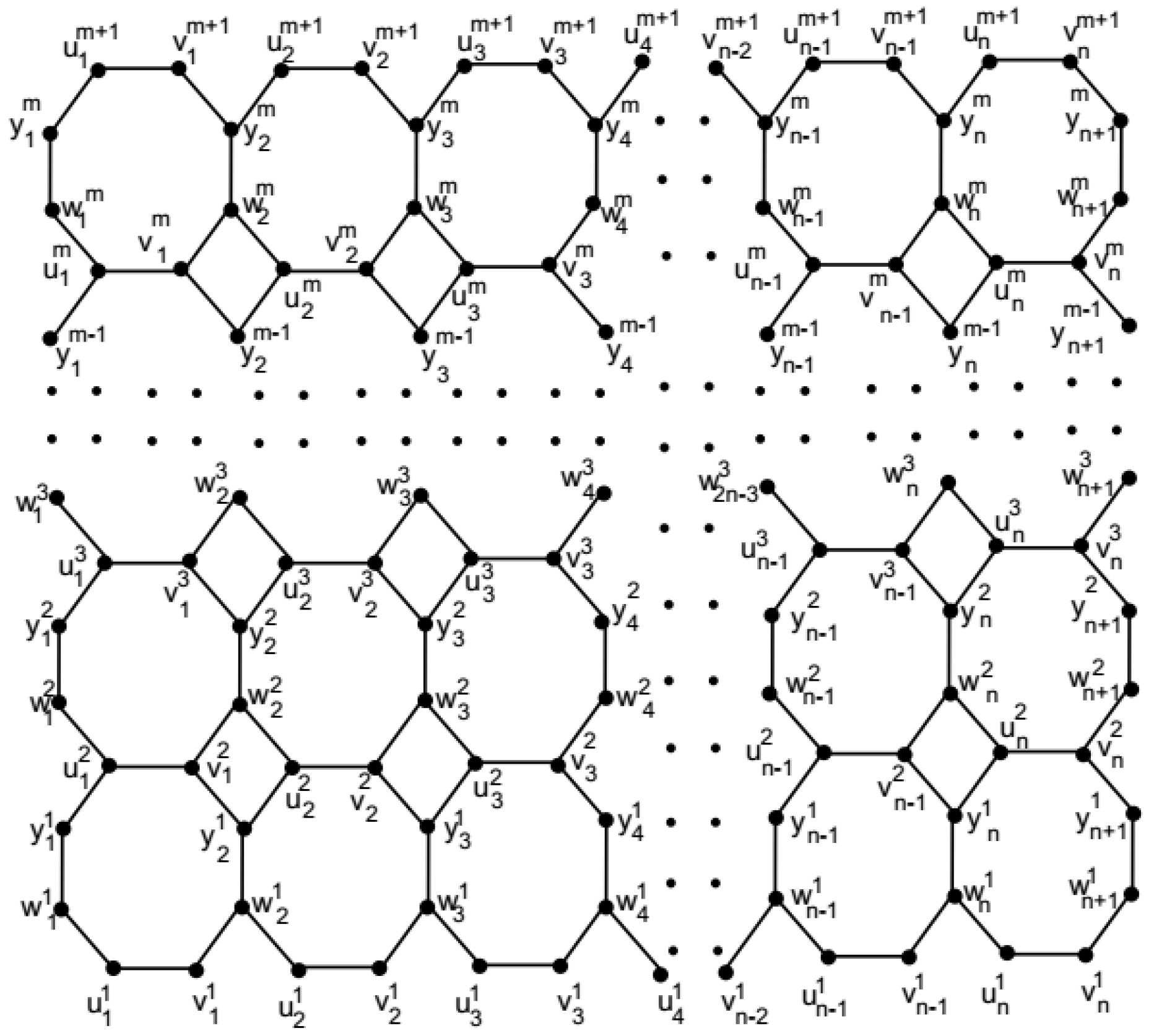
3. The Octagonal Grid O n m

In [19,20], Diudea et al. constructed a C 4 C 8 net as a trivalent decoration made by alternating squares C 4 and octagons C 8 in two different ways. One is by alternating squares C 4 and octagons C 8 in different ways denoted by C 4 C 8 ( S ) and the other is by alternating rhombus and octagons in different ways denoted by C 4 C 8 ( R ) . We denote C 4 C 8 ( R ) by O n m (see Figure 1). In [21,22], they also called it the Octagonal grid.
For n , m 3 , the Octagonal grid O n m is the grid with m rows and n columns of octagons. The symbols V ( O n m ) and E ( O n m ) denote the vertex set and the edge set of O n m , respectively.
V ( O n m ) = { u s t : 1 s n , 1 t m + 1 } { v s t : 1 s n ; 1 t m + 1 } { w s t : 1 s n + 1 , 1 t m } { y s t : 1 s n + 1 , 1 t m } .
E ( O n m ) = { u s t v s t : 1 s n , 1 t m + 1 } { u s t w s t : 1 s n , 1 t m } { w s t y s t : 1 s n + 1 , 1 t m } { v s t w s + 1 t : 1 s n , 1 t m } { v s t y s + 1 t 1 : 1 s n , 2 t m + 1 } { u s t + 1 y s t : 1 s n , 2 t m } .
In this paper, we consider O n m with n = m . and we compute Connective Eccentric index C ξ ( G ) , Eccentric connectivity index ξ ( G ) and eccentric Zagreb indices of O n m . For this, we discuss two cases of n, when n 0 ( m o d 2 ) and when n 1 ( m o d 2 ) .
Theorem 1.
For every n 4 and n 0 ( m o d 2 ) , consider the graph of G O n m , with n = m . Then, the Connective Eccentric index of G is equal to:
C ξ ( G ) = 32 14 n + 1 7 n ( 7 n + 1 ) + 16 s = 1 n 2 1 1 4 n + 1 s + 2 7 n + 2 s + s = 1 n 2 t = s + 1 n 2 + 1 12 4 n 3 ( s 1 ) t + s = 2 n 2 t = 2 s 12 4 ( n + 1 ) s 3 t + s = n 2 + 1 n 1 t = 2 n s + 1 12 3 ( n t ) + s + 2 + s = n 2 + 2 n t = n s + 2 n 2 + 1 12 n + 3 s t 1 + s = 1 n 2 1 t = n 2 + 2 n s + 1 12 3 ( n s ) + t + 1 + s = 2 n 2 t = n + 2 s n 12 n s + 3 t 2 + s = n 2 + 2 n t = n 2 + 2 s 12 4 s + t n 3 + s = n 2 + 1 n 1 t = s + 1 n 12 s + 3 t 4 .
Proof. 
Let G be the graph of O n m . Note that graph of O n m is a symmetric about reflection and rotation at right angles. Thus, the eccentricities ε u s t = ε v n + 1 s t and from the symmetry at right angles we can obtain that the eccentricities ε y s t = ε u t s , ε w s t = ε v t s . Therefore, from Equation (1), the Connective Eccentric index of O n m is equal to
C ξ ( O n m ) = 4 u s t V ( G ) d u s t ε u s t
By using the values in Table 1, we get
C ξ ( O n m ) = 4 2 s = 1 n 2 + 1 2 4 n + 1 s + 2 s = n 2 + 2 n 2 3 n + s 1 + 4 [ s = 1 n 2 t = s + 1 n 2 + 1 3 4 n 3 ( s 1 ) t + s = 2 n 2 t = 2 s 3 4 ( n + 1 ) s 3 t + s = n 2 + 1 n 1 t = 2 n s + 1 3 3 ( n t ) + s + 2 + s = 1 n 2 1 t = n 2 + 2 n s + 1 3 3 ( n s ) + t + 1 + s = 2 n 2 t = n + 2 s n 3 n s + 3 t 2 + s = n 2 + 2 n t = n 2 + 2 s 3 4 s + t n 3 + s = n 2 + 1 n 1 t = s + 1 n 3 s + 3 t 4 ] + s = n 2 + 2 n t = n s + 2 n 2 + 1 3 n + 3 s t 1 .
After an easy computation, we get
C ξ ( G ) = 32 14 n + 1 7 n ( 7 n + 1 ) + 16 s = 1 n 2 1 1 4 n + 1 s + 2 7 n + 2 s + s = 1 n 2 t = s + 1 n 2 + 1 12 4 n 3 ( s 1 ) t + s = 2 n 2 t = 2 s 12 4 ( n + 1 ) s 3 t + s = n 2 + 1 n 1 t = 2 n s + 1 12 3 ( n t ) + s + 2 + s = n 2 + 2 n t = n s + 2 n 2 + 1 12 n + 3 s t 1 + s = 1 n 2 1 t = n 2 + 2 n s + 1 12 3 ( n s ) + t + 1 + s = 2 n 2 t = n + 2 s n 12 n s + 3 t 2 + s = n 2 + 2 n t = n 2 + 2 s 12 4 s + t n 3 + s = n 2 + 1 n 1 t = s + 1 n 12 s + 3 t 4 .
 ☐
Theorem 2.
For every n 3 and n 1 ( m o d 2 ) , consider the graph of G O n m , with n = m . Then, the Connective Eccentric index of G is equal to
C ξ ( G ) = 32 7 n + 1 + 16 s = 1 n + 1 2 1 1 4 n + 1 s + 2 5 n 2 s 3 + s = 1 n + 1 2 1 t = s + 1 n + 1 2 12 4 n 3 ( s 1 ) t + s = 2 n + 1 2 t = 2 s 12 4 ( n + 1 ) s 3 t + s = n + 1 2 + 1 n 1 t = 2 n s + 1 12 3 ( n t ) + s + 2 + s = n + 1 2 + 1 n t = n s + 2 n + 1 2 12 n + 3 s t 1 v + s = 1 n + 1 2 1 t = n + 1 2 + 1 n s + 1 12 3 ( n s ) + t + 1 + s = 2 n + 1 2 t = n + 2 s n 12 n s + 3 t 2 + s = n + 1 2 + 1 n t = n + 1 2 + 1 s 12 4 s + t n 3 + s = n + 1 2 + 1 n 1 t = s + 1 n 12 s + 3 t 4 .
Proof. 
Let G be the graph of O n m and n 3 is odd. As above noted, the graph of O n m is a symmetric about reflection and rotation at right angles. Thus, the eccentricities ε u s t = ε v n + 1 s t and from the symmetry at right angles we can obtain that the eccentricities ε y s t = ε u t s , ε w s t = ε v t s . Therefore, from Equation (1), the Connective Eccentric index of O n m is equal to
C ξ ( O n m ) = 4 u s t V ( G ) d u s t ε u s t
By using the values in Table 2, we get
C ξ ( G ) = C ξ ( O n m ) = 4 2 s = 1 n + 1 2 2 4 n + 1 s + 2 s = n + 1 2 + 1 n 2 3 n + s 1 + 4 [ s = 1 n + 1 2 1 t = s + 1 n + 1 2 3 4 n 3 ( s 1 ) t + s = 2 n + 1 2 t = 2 s 3 4 ( n + 1 ) s 3 t + s = n + 1 2 + 1 n 1 t = 2 n s + 1 3 3 ( n t ) + s + 2 + s = n + 1 2 + 1 n t = n s + 2 n + 1 2 3 n + 3 s t 1 + s = 1 n + 1 2 1 t = n + 1 2 + 1 n s + 1 3 3 ( n s ) + t + 1 + s = 2 n + 1 2 t = n + 2 s n 3 n s + 3 t 2 + s = n + 1 2 + 1 n t = n + 1 2 + 1 s 3 4 s + t n 3 + s = n + 1 2 + 1 n 1 t = s + 1 n 3 s + 3 t 4 ] .
After an easy computation, we get
C ξ ( G ) = 32 7 n + 1 + 16 s = 1 n + 1 2 1 1 4 n + 1 s + 2 5 n 2 s 3 + s = 1 n + 1 2 1 t = s + 1 n + 1 2 12 4 n 3 ( s 1 ) t + s = 2 n + 1 2 t = 2 s 12 4 ( n + 1 ) s 3 t + s = n + 1 2 + 1 n 1 t = 2 n s + 1 12 3 ( n t ) + s + 2 + s = n + 1 2 + 1 n t = n s + 2 n + 1 2 12 n + 3 s t 1 + s = 1 n + 1 2 1 t = n + 1 2 + 1 n s + 1 12 3 ( n s ) + t + 1 + s = 2 n + 1 2 t = n + 2 s n 12 n s + 3 t 2 + s = n + 1 2 + 1 n t = n + 1 2 + 1 s 12 4 s + t n 3 + s = n + 1 2 + 1 n 1 t = s + 1 n 12 s + 3 t 4 .
 ☐
Theorem 3.
For every n 4 and n 0 ( m o d 2 ) , consider the graph of G O n m , with n = m . Then, the Eccentric Connectivity index of G is equal to
ξ ( G ) = 60 n 2 + s = 1 n 2 t = s + 1 n 2 + 1 12 { 4 n 3 ( s 1 ) t } + s = 2 n 2 t = 2 s 12 { 4 ( n + 1 ) s 3 t } + s = n 2 + 1 n 1 t = 2 n s + 1 12 { 3 ( n t ) + s + 2 } + s = n 2 + 2 n t = n s + 2 n 2 + 1 12 { n + 3 s t 1 } + s = 1 n 2 1 t = n 2 + 2 n s + 1 12 { 3 ( n s ) + t + 1 } + s = 2 n 2 t = n + 2 s n 12 { n s + 3 t 2 } + s = n 2 + 2 n t = n 2 + 2 s 12 { 4 s + t n 3 } + s = n 2 + 1 n 1 t = s + 1 n 12 { s + 3 t 4 } .
Proof. 
By using the arguments in the proof of Theorem 1, the values in Table 1 and Equation (2), we get
ξ ( G ) = ξ ( O n m ) = 4 2 s = 1 n 2 + 1 2 { 4 n + 1 s } + 2 s = n 2 + 2 n 2 { 3 n + s 1 } + 4 [ s = 1 n 2 t = s + 1 n 2 + 1 3 { 4 n 3 ( s 1 ) t } + s = 2 n 2 t = 2 s 3 { 4 ( n + 1 ) s 3 t } + s = n 2 + 1 n 1 t = 2 n s + 1 3 { 3 ( n t ) + s + 2 } + s = n 2 + 2 n t = n s + 2 n 2 + 1 3 { n + 3 s t 1 } + s = 1 n 2 1 t = n 2 + 2 n s + 1 3 { 3 ( n s ) + t + 1 } + s = 2 n 2 t = n + 2 s n 3 { n s + 3 t 2 } + s = n 2 + 2 n t = n 2 + 2 s 3 { 4 s + t n 3 } + s = n 2 + 1 n 1 t = s + 1 n 3 { s + 3 t 4 } ] .
After some easy calculations, we get
ξ ( G ) = 60 n 2 + s = 1 n 2 t = s + 1 n 2 + 1 12 { 4 n 3 ( s 1 ) t } + s = 2 n 2 t = 2 s 12 { 4 ( n + 1 ) s 3 t } + s = n 2 + 1 n 1 t = 2 n s + 1 12 { 3 ( n t ) + s + 2 } + s = n 2 + 2 n t = n s + 2 n 2 + 1 12 { n + 3 s t 1 } + s = 1 n 2 1 t = n 2 + 2 n s + 1 12 { 3 ( n s ) + t + 1 } + s = 2 n 2 t = n + 2 s n 12 { n s + 3 t 2 } + s = n 2 + 2 n t = n 2 + 2 s 12 { 4 s + t n 3 } + s = n 2 + 1 n 1 t = s + 1 n 12 { s + 3 t 4 } .
 ☐
Theorem 4.
For every n 3 and n 1 ( m o d 2 ) , consider the graph of G O n m , with n = m . Then, the Eccentric Connectivity index of G is equal to
ξ ( G ) = 60 n 2 32 n + 10 + s = 1 n + 1 2 1 t = s + 1 n + 1 2 12 { 4 n 3 ( s 1 ) t } + s = 2 n + 1 2 t = 2 s 12 { 4 ( n + 1 ) s 3 t } + s = n + 1 2 + 1 n 1 t = 2 n s + 1 12 { 3 ( n t ) + s + 2 } + s = n + 1 2 + 1 n t = n s + 2 n + 1 2 12 { n + 3 s t 1 } + s = 1 n + 1 2 1 t = n + 1 2 + 1 n s + 1 12 { 3 ( n s ) + t + 1 } + s = 2 n + 1 2 t = n + 2 s n 12 { n s + 3 t 2 } + s = n + 1 2 + 1 n t = n + 1 2 + 1 s 12 { 4 s + t n 3 } + s = n + 1 2 + 1 n 1 t = s + 1 n 12 { s + 3 t 4 } .
Proof. 
By using the arguments in the proof of Theorem 2, the values in Table 2 and Equation (2), we get
ξ ( G ) = ξ ( O n m ) = 4 2 s = 1 n + 1 2 2 { 4 n + 1 s } + 2 s = n + 1 2 + 1 n 2 { 3 n + s 1 } + 4 [ s = 1 n + 1 2 1 t = s + 1 n + 1 2 3 { 4 n 3 ( s 1 ) t } + s = 2 n + 1 2 t = 2 s 3 { 4 ( n + 1 ) s 3 t } + s = n + 1 2 + 1 n 1 t = 2 n s + 1 3 { 3 ( n t ) + s + 2 } + s = n + 1 2 + 1 n t = n s + 2 n + 1 2 3 { n + 3 s t 1 } + s = 1 n + 1 2 1 t = n + 1 2 + 1 n s + 1 3 { 3 ( n s ) + t + 1 } + s = 2 n + 1 2 t = n + 2 s n 3 { n s + 3 t 2 } + s = n + 1 2 + 1 n t = n + 1 2 + 1 s 3 { 4 s + t n 3 } + s = n + 1 2 + 1 n 1 t = s + 1 n 3 { s + 3 t 4 } ] .
After some easy calculations, we get
ξ ( G ) = 60 n 2 32 n + 10 + s = 1 n + 1 2 1 t = s + 1 n + 1 2 12 { 4 n 3 ( s 1 ) t } + s = 2 n + 1 2 t = 2 s 12 { 4 ( n + 1 ) s 3 t } + s = n + 1 2 + 1 n 1 t = 2 n s + 1 12 { 3 ( n t ) + s + 2 } + s = n + 1 2 + 1 n t = n s + 2 n + 1 2 12 { n + 3 s t 1 } + s = 1 n + 1 2 1 t = n + 1 2 + 1 n s + 1 12 { 3 ( n s ) + t + 1 } + s = 2 n + 1 2 t = n + 2 s n 12 { n s + 3 t 2 } + s = n + 1 2 + 1 n t = n + 1 2 + 1 s 12 { 4 s + t n 3 } + s = n + 1 2 + 1 n 1 t = s + 1 n 12 { s + 3 t 4 } .
 ☐
Theorem 5.
For every n 4 and n 0 ( m o d 2 ) , consider the graph of G O n m , with n = m . Then, the eccentric Zagreb index of G is equal to
M 1 ( O n m ) = 338 3 n 3 + 4 n 3 + 4 [ s = 1 n 2 t = s + 1 n 2 + 1 ( 4 n 3 ( s 1 ) t ) 2 + s = 2 n 2 t = 2 s ( 4 ( n + 1 ) s 3 t ) 2 + s = n 2 + 1 n 1 t = 2 n s + 1 ( 3 ( n t ) + s + 2 ) 2 + s = n 2 + 2 n t = n s + 2 n 2 + 1 ( n + 3 s t 1 ) 2 + s = 1 n 2 1 t = n 2 + 2 n s + 1 ( 3 ( n s ) + t + 1 ) 2 + s = 2 n 2 t = n + 2 s n ( n s + 3 t 2 ) 2 + s = n 2 + 2 n t = n 2 + 2 s ( 4 s + t n 3 ) 2 + s = n 2 + 1 n 1 t = s + 1 n ( s + 3 t 4 ) 2 ] .
Proof. 
By using the arguments in the proof of Theorem 1, the values in Table 1 and the following equation, we get
M 1 ( G ) = u V ( G ) ( ϵ u ) 2 ,
M 1 ( O n m ) = 4 u s t V ( G ) ( ε u s t ) 2 = 4 2 s = 1 n 2 + 1 ( 4 n + 1 s ) 2 + 2 s = n 2 + 2 n ( 3 n + s 1 ) 2 + 4 [ s = 1 n 2 t = s + 1 n 2 + 1 ( 4 n 3 ( s 1 ) t ) 2 + s = 2 n 2 t = 2 s ( 4 ( n + 1 ) s 3 t ) 2 + s = n 2 + 1 n 1 t = 2 n s + 1 ( 3 ( n t ) + s + 2 ) 2 + s = n 2 + 2 n t = n s + 2 n 2 + 1 ( n + 3 s t 1 ) 2 + s = 1 n 2 1 t = n 2 + 2 n s + 1 ( 3 ( n s ) + t + 1 ) 2 + s = 2 n 2 t = n + 2 s n ( n s + 3 t 2 ) 2 + s = n 2 + 2 n t = n 2 + 2 s ( 4 s + t n 3 ) 2 + s = n 2 + 1 n 1 t = s + 1 n ( s + 3 t 4 ) 2 ] .
After some easy calculations, we get
M 1 ( O n m ) = 338 3 n 3 + 4 n 3 + 4 [ s = 1 n 2 t = s + 1 n 2 + 1 ( 4 n 3 ( s 1 ) t ) 2 + s = 2 n 2 t = 2 s ( 4 ( n + 1 ) s 3 t ) 2 + s = n 2 + 1 n 1 t = 2 n s + 1 ( 3 ( n t ) + s + 2 ) 2 + s = n 2 + 2 n t = n s + 2 n 2 + 1 ( n + 3 s t 1 ) 2 + s = 1 n 2 1 t = n 2 + 2 n s + 1 ( 3 ( n s ) + t + 1 ) 2 + s = 2 n 2 t = n + 2 s n ( n s + 3 t 2 ) 2 + s = n 2 + 2 n t = n 2 + 2 s ( 4 s + t n 3 ) 2 + s = n 2 + 1 n 1 t = s + 1 n ( s + 3 t 4 ) 2 ] .
 ☐
Theorem 6.
For every n 3 and n 1 ( m o d 2 ) , consider the graph of G O n m , with n = m . Then, the eccentric Zagreb index of G is equal to
M 1 ( O n m ) = 338 3 n 3 + 46 n 3 + 4 [ s = 1 n + 1 2 1 t = s + 1 n + 1 2 ( 4 n 3 ( s 1 ) t ) 2 + s = 2 n + 1 2 t = 2 s ( 4 ( n + 1 ) s 3 t ) 2 + s = n + 1 2 + 1 n 1 t = 2 n s + 1 ( 3 ( n t ) + s + 2 ) 2 + s = n + 1 2 + 1 n t = n s + 2 n + 1 2 ( n + 3 s t 1 ) 2 + s = 1 n + 1 2 1 t = n + 1 2 + 1 n s + 1 ( 3 ( n s ) + t + 1 ) 2 + s = 2 n + 1 2 t = n + 2 s n ( n s + 3 t 2 ) 2 + s = n + 1 2 + 1 n t = n + 1 2 + 1 s ( 4 s + t n 3 ) 2 + s = n + 1 2 + 1 n 1 t = s + 1 n ( s + 3 t 4 ) 2 ]
Proof. 
By using the arguments in the proof of Theorem 1, the values in Table 2 and the following equation, we get
M 1 ( G ) = u V ( G ) ( ϵ u ) 2 ,
M 1 ( O n m ) = 4 u s t V ( G ) ( ε u s t ) 2 = 4 2 s = 1 n + 1 2 ( 4 n + 1 s ) 2 + 2 s = n + 1 2 + 1 n ( 3 n + s 1 ) 2 + 4 [ s = 1 n + 1 2 1 t = s + 1 n + 1 2 ( 4 n 3 ( s 1 ) t ) 2 + s = 2 n + 1 2 t = 2 s ( 4 ( n + 1 ) s 3 t ) 2 + s = n + 1 2 + 1 n 1 t = 2 n s + 1 ( 3 ( n t ) + s + 2 ) 2 + s = n + 1 2 + 1 n t = n s + 2 n + 1 2 ( n + 3 s t 1 ) 2 + s = 1 n + 1 2 1 t = n + 1 2 + 1 n s + 1 ( 3 ( n s ) + t + 1 ) 2 + s = 2 n + 1 2 t = n + 2 s n ( n s + 3 t 2 ) 2 + s = n + 1 2 + 1 n t = n + 1 2 + 1 s ( 4 s + t n 3 ) 2 + s = n + 1 2 + 1 n 1 t = s + 1 n ( s + 3 t 4 ) 2 ] .
After some easy calculations, we get
M 1 ( O n m ) = 338 3 n 3 + 46 n 3 + 4 [ s = 1 n + 1 2 1 t = s + 1 n + 1 2 ( 4 n 3 ( s 1 ) t ) 2 + s = 2 n + 1 2 t = 2 s ( 4 ( n + 1 ) s 3 t ) 2 + s = n + 1 2 + 1 n 1 t = 2 n s + 1 ( 3 ( n t ) + s + 2 ) 2 + s = n + 1 2 + 1 n t = n s + 2 n + 1 2 ( n + 3 s t 1 ) 2 + s = 1 n + 1 2 1 t = n + 1 2 + 1 n s + 1 ( 3 ( n s ) + t + 1 ) 2 + s = 2 n + 1 2 t = n + 2 s n ( n s + 3 t 2 ) 2 + s = n + 1 2 + 1 n t = n + 1 2 + 1 s ( 4 s + t n 3 ) 2 + s = n + 1 2 + 1 n 1 t = s + 1 n ( s + 3 t 4 ) 2 ] .
 ☐
Theorem 7.
For every n 4 and n 0 ( m o d 2 ) , consider the graph of G O n m , with n = m . Then, the Eccentric Connectivity Polynomial of G is equal to
E C P ( O n m , x ) = 1 ( x 1 ) 16 x ( 7 n 2 + 1 ) + 16 x ( 4 n + 1 ) + 16 1 x n 2 + 16 x 4 n + 4 [ s = 1 n 2 t = s + 1 n 2 + 1 3 x ( 4 n 3 ( s 1 ) t ) + s = 2 n 2 t = 2 s 3 x ( 4 ( n + 1 ) s 3 t ) + s = n 2 + 1 n 1 t = 2 n s + 1 3 x ( 3 ( n t ) + s + 2 ) + s = n 2 + 2 n t = n s + 2 n 2 + 1 3 x ( n + 3 s t 1 ) + s = 1 n 2 1 t = n 2 + 2 n s + 1 3 x ( 3 ( n s ) + t + 1 ) + s = 2 n 2 t = n + 2 s n 3 x ( n s + 3 t 2 ) + s = n 2 + 2 n t = n 2 + 2 s 3 x ( 4 s + t n 3 ) + s = n 2 + 1 n 1 t = s + 1 n 3 x ( s + 3 t 4 ) ] .
Proof. 
By using the arguments in the proof of Theorem 1, the values in Table 1 and Equation (4) we get
E C P ( O n m , x ) = 4 2 s = 1 n 2 + 1 2 x ( 4 n + 1 s ) + 2 s = n 2 + 2 n 2 x ( 3 n + s 1 ) + 4 [ s = 1 n 2 t = s + 1 n 2 + 1 3 x ( 4 n 3 ( s 1 ) t ) + s = 2 n 2 t = 2 s 3 x ( 4 ( n + 1 ) s 3 t ) + s = n 2 + 1 n 1 t = 2 n s + 1 3 x ( 3 ( n t ) + s + 2 ) + s = n 2 + 2 n t = n s + 2 n 2 + 1 3 x ( n + 3 s t 1 ) + s = 1 n 2 1 t = n 2 + 2 n s + 1 3 x ( 3 ( n s ) + t + 1 ) + s = 2 n 2 t = n + 2 s n 3 x ( n s + 3 t 2 ) + s = n 2 + 2 n t = n 2 + 2 s 3 x ( 4 s + t n 3 ) + s = n 2 + 1 n 1 t = s + 1 n 3 x ( s + 3 t 4 ) ] .
After some easy calculations, we get
E C P ( O n m , x ) = 1 ( x 1 ) 16 x ( 7 n 2 + 1 ) + 16 x ( 4 n + 1 ) + 16 1 x n 2 + 16 x 4 n + 4 [ s = 1 n 2 t = s + 1 n 2 + 1 3 x ( 4 n 3 ( s 1 ) t ) + s = 2 n 2 t = 2 s 3 x ( 4 ( n + 1 ) s 3 t ) + s = n 2 + 1 n 1 t = 2 n s + 1 3 x ( 3 ( n t ) + s + 2 ) + s = n 2 + 2 n t = n s + 2 n 2 + 1 3 x ( n + 3 s t 1 ) + s = 1 n 2 1 t = n 2 + 2 n s + 1 3 x ( 3 ( n s ) + t + 1 ) + s = 2 n 2 t = n + 2 s n 3 x ( n s + 3 t 2 ) + s = n 2 + 2 n t = n 2 + 2 s 3 x ( 4 s + t n 3 ) + s = n 2 + 1 n 1 t = s + 1 n 3 x ( s + 3 t 4 ) ] .
 ☐
Theorem 8.
For every n 3 and n 1 ( m o d 2 ) , consider the graph of G O n m , with n = m . Then, the Eccentric Connectivity Polynomial of G is equal to
E C P ( O n m , x ) = 1 ( x 1 ) 32 x ( 7 n + 1 2 ) + 16 x ( 4 n + 1 ) + 16 x ( 4 n ) + 4 [ s = 1 n + 1 2 1 t = s + 1 n + 1 2 3 x ( 4 n 3 ( s 1 ) t ) + s = 2 n + 1 2 t = 2 s 3 x ( 4 ( n + 1 ) s 3 t ) + s = n + 1 2 + 1 n 1 t = 2 n s + 1 3 x ( 3 ( n t ) + s + 2 ) + s = n + 1 2 + 1 n t = n s + 2 n + 1 2 3 x ( n + 3 s t 1 ) + s = 1 n + 1 2 1 t = n + 1 2 + 1 n s + 1 3 x ( 3 ( n s ) + t + 1 ) + s = 2 n + 1 2 t = n + 2 s n 3 x ( n s + 3 t 2 ) + s = n + 1 2 + 1 n t = n + 1 2 + 1 s 3 x ( 4 s + t n 3 ) + s = n + 1 2 + 1 n 1 t = s + 1 n 3 x ( s + 3 t 4 ) ] .
Proof. 
By using the arguments in the proof of Theorem 1, the values in Table 2 and Equation (4), we get
E C P ( O n m , x ) = 4 2 s = 1 n + 1 2 2 x ( 4 n + 1 s ) + 2 s = n + 1 2 + 1 n 2 x ( 3 n + s 1 ) + 4 [ s = 1 n + 1 2 1 t = s + 1 n + 1 2 3 x ( 4 n 3 ( s 1 ) t ) + s = 2 n + 1 2 t = 2 s 3 x ( 4 ( n + 1 ) s 3 t ) + s = n + 1 2 + 1 n 1 t = 2 n s + 1 3 x ( 3 ( n t ) + s + 2 ) + s = n + 1 2 + 1 n t = n s + 2 n + 1 2 3 x ( n + 3 s t 1 ) + s = 1 n + 1 2 1 t = n + 1 2 + 1 n s + 1 3 x ( 3 ( n s ) + t + 1 ) + s = 2 n + 1 2 t = n + 2 s n 3 x ( n s + 3 t 2 ) + s = n + 1 2 + 1 n t = n + 1 2 + 1 s 3 x ( 4 s + t n 3 ) + s = n + 1 2 + 1 n 1 t = s + 1 n 3 x ( s + 3 t 4 ) ] .
After some easy calculations, we get
E C P ( O n m , x ) = 1 ( x 1 ) 32 x ( 7 n + 1 2 ) + 16 x ( 4 n + 1 ) + 16 x ( 4 n ) + 4 [ s = 1 n + 1 2 1 t = s + 1 n + 1 2 3 x ( 4 n 3 ( s 1 ) t ) + s = 2 n + 1 2 t = 2 s 3 x ( 4 ( n + 1 ) s 3 t ) + s = n + 1 2 + 1 n 1 t = 2 n s + 1 3 x ( 3 ( n t ) + s + 2 ) + s = n + 1 2 + 1 n t = n s + 2 n + 1 2 3 x ( n + 3 s t 1 ) + s = 1 n + 1 2 1 t = n + 1 2 + 1 n s + 1 3 x ( 3 ( n s ) + t + 1 ) + s = 2 n + 1 2 t = n + 2 s n 3 x ( n s + 3 t 2 ) + s = n + 1 2 + 1 n t = n + 1 2 + 1 s 3 x ( 4 s + t n 3 ) + s = n + 1 2 + 1 n 1 t = s + 1 n 3 x ( s + 3 t 4 ) ] .
 ☐

4. Conclusions

In this paper, we discuss the Octagonal Grid and compute the eccentric connectivity index, eccentricity Zagreb index, connective eccentric index and eccentric connectivity polynomial of the Octagonal grid of O n m . Since eccentricity based indices have various applications in nanomedicine and materials science, these theoretical results could have applications in medical science.

Author Contributions

X.Z. contributed for supervision, project administration, funding and analyzed the data curation. M.K.S. contributed for designing the experiments, validation, conceptualization, formal analysing experiments, resources, software and some computations. M.N. and A.Q.B. contributed for Investigation, Methodology wrote the initial draft of the paper. M.K.S. investigated and wrote the final draft. All authors read and approved the final version of the paper.

Funding

This work was supported by Applied Basic Research (Key Project) of the Sichuan Province under grant 2017JY0095, the key project of the Sichuan Provincial Department of Education under grant 17ZA0079 and 18ZA0118, the Soft Scientific Research Foundation of Sichuan Provincial Science and Technology Department (18RKX1048).

Conflicts of Interest

The authors declare no conflicts of interest.

References

  1. Wiener, H. Correlation of heat of isomerization and difierence in heat of vaporization of isomers among paran hydrocaibons. J. Am. Chem. Soc. 1947, 69, 2636–2638. [Google Scholar] [CrossRef]
  2. Wiener, H. Influence of interatomic forces on para–n properties. J. Chem. Phys. 1947, 15, 766–767. [Google Scholar] [CrossRef]
  3. Wiener, H. Vapour-pressure-temperature relations among the branched para–n hydrocarbons. J. Chem. Phys. 1948, 15, 425–430. [Google Scholar] [CrossRef]
  4. Hosoya, H. Topological index. Newly proposed quautity characterizing the topological nature of structure of isomers of saturated hydrocarbons. Bull. Chem. Soc. Jpn. 1971, 44, 2332–2337. [Google Scholar] [CrossRef]
  5. Hosoya, H. Topological index as strong sorting device for coding chemical structure. J. Chem. Doc. 1972, 12, 181–183. [Google Scholar] [CrossRef]
  6. Randić, M. On characterization of molecular branching. J. Am. Chem. Soc. 1975, 97, 6609–6615. [Google Scholar]
  7. Došlić, T.; Saheli, M. Eccentric connectivity index of composite graphs. Util. Math. 2014, 95, 3–22. [Google Scholar]
  8. Gupta, S.; Singh, M.; Madan, A.K. Connective eccentricity index: A novel topological descriptor for predicting biological activity. J. Mol. Graph. Model. 2000, 18, 18–28. [Google Scholar] [CrossRef]
  9. Yu, G.; Qu, H.; Tang, L.; Feng, L. On the connective eccentricity index of trees and unicyclic graphs with given diameter. J. Math. Anal. Appl. 2014, 420, 1776–1786. [Google Scholar] [CrossRef]
  10. Huo, Y.; Liu, J.B.; Baig, A.Q.; Sajjad, W.; Farahani, M.R. Connective Eccentric Index of N A n m Nanotube. J. Comput. Theor. Nanosci. 2017, 14, 1832–1836. [Google Scholar] [CrossRef]
  11. Siddiqui, M.K.; Gharibi, W. On Zagreb Indices, Zagreb Polynomials of Mesh Derived Networks. J. Comput. Theor. Nanosci. 2016, 13, 8683–8688. [Google Scholar] [CrossRef]
  12. Siddiqui, M.K.; Imran, M.; Ahmad, A. On Zagreb indices, Zagreb polynomials of some nanostar dendrimers. Appl. Math. Comput. 2016, 280, 132–139. [Google Scholar] [CrossRef]
  13. Gao, W.; Siddiqui, M.K. Molecular Descriptors of Nanotube, Oxide, Silicate, and Triangulene networks. J. Chem. 2017, 2017, 1–10. [Google Scholar] [CrossRef]
  14. Gao, W.; Siddiqui, M.K.; Naeem, M.; Rehman, N.A. Topological Characterization of Carbon Graphite and Crystal Cubic Carbon Structures. Molecules 2017, 22, 1496. [Google Scholar] [CrossRef] [PubMed]
  15. Idrees, N.; Naeem, M.N.; Hussain, F.; Sadiq, A.; Siddiqui, M.K. Molecular Descriptors of Benzenoid System. Quim. Nova 2017, 40, 143–145. [Google Scholar] [CrossRef]
  16. Zhou, B.; Du, Z. On eccentric connectivity index. MATCH Commun. Math. Comput. Chem. 2010, 63, 181–198. [Google Scholar]
  17. Ghorbani, M.; Hosseinzadeh, M.A. A New Version of Zagreb Indices. Filomat 2012, 26, 93–100. [Google Scholar] [CrossRef]
  18. Alaeiyan, M.; Mojarad, R.; Asadpour, J. A new method for computing eccentric connectivity polynomial of an infinite family of linear polycene parallelogram benzenod. Optoelectron. Adv. Mater.-Rapid Commun. 2011, 5, 761–763. [Google Scholar]
  19. Diudea, M.V. Nanostructures: Novel Architecture; Nova Science Publishers: New York, NY, USA, 2005; pp. 203–242. [Google Scholar]
  20. Stefu, M.; Diudea, M.V. Wiener index of C4C8 nanotubes. MATCH Commun. Math. Comput. Chem. 2004, 50, 133–143. [Google Scholar]
  21. Siddiqui, M.K.; Naeem, M.; Rahman, N.A.; Imran, M. Computing topological indices of certain networks. J. Optoelctron. Adv. Mater. 2016, 18, 884–892. [Google Scholar]
  22. Siddiqui, M.K.; Miller, M.; Ryan, J. Total edge irregularity strength of octagonal grid graph. Util. Math. 2017, 103, 277–287. [Google Scholar]
Figure 1. The Octagonal grid O n m .
Mathematics 06 00153 g001
Table 1. Partition of vertices of the type u s t of O n m based on degree and eccentricity of each vertex when n 0 ( m o d 2 ) .
RepresentativeDegreeEccentricityRangeFrequency
u s t 2 4 n s + 1 t = 1 , n + 1 , 2 ( n + 2 2 )
1 s n 2 + 1
u s t 2 3 n + s 1 t = 1 , n + 1 , 2 ( n 2 2 )
n 2 + 2 s n
u s t 3 4 n 3 ( s 1 ) t 1 s n 2 , n 4 ( n 2 + 1 )
s + 1 t n 2 + 1
u s t 3 4 ( n + 1 ) s 3 t 2 s n 2 , n 4 ( n 2 + 1 )
2 t s
u s t 3 3 n + s 3 t + 2 n 2 + 1 s n 1 , n 4 ( n 2 1 )
2 t n + 1 s
u s t 3 n + 3 s t 1 n 2 + 2 s n , n 4 ( n 2 1 )
n s + 2 t n 2 + 1
u s t 3 3 ( n s ) + t + 1 1 s n 2 1 , 1 2 ( n 2 2 ) ( n 2 1 )
n 2 + 2 t n s + 1
u s t 3 n s + 3 t 2 2 s n 2 , 1 2 ( n 2 2 ) ( n 2 1 )
n s + 2 t n
u s t 3 4 s n + t 3 n 2 + 2 s n , n 4 ( n 2 1 )
n 2 + 2 t s
u s t 3 s + 3 t 4 n 2 + 1 s n 1 , n 4 ( n 2 1 )
s + 1 t n
Table 2. Partition of vertices of the type u s t of O n m based on degree and eccentricity of each vertex when n 1 ( m o d 2 ) .
RepresentativeDegreeEccentricityRangeFrequency
u s t 2 4 n s + 1 t = 1 , n + 1 , 2 ( n + 1 2 )
1 s n + 1 2
u s t 2 3 n + s 1 t = 1 , n + 1 , 2 ( n 1 2 )
n + 1 2 + 1 s n
u s t 3 4 n 3 ( s 1 ) t 1 s n + 1 2 1 , n + 1 4 ( n + 1 2 1 )
s + 1 t n + 1 2
u s t 3 4 ( n + 1 ) s 3 t 2 s n + 1 2 , n + 1 4 ( n + 1 2 1 )
2 t s
u s t 3 3 n + s 3 t + 2 n + 1 2 + 1 s n 1 , n 1 4 ( n 1 2 1 )
2 t n + 1 s
u s t 3 n + 3 s t 1 n + 1 2 + 1 s n , n 1 4 ( n 1 2 + 1 )
n s + 2 t n + 1 2
u s t 3 3 ( n s ) + t + 1 1 s n + 1 2 1 , n + 1 4 ( n + 1 2 1 )
n + 1 2 + 1 t n s + 1
u s t 3 n s + 3 t 2 2 s n + 1 2 , n + 1 4 ( n + 1 2 1 )
n s + 2 t n
u s t 3 4 s n + t 3 n + 1 2 + 1 s n , n 1 4 ( n + 1 2 )
n + 1 2 + 1 t s
u s t 3 s + 3 t 4 n + 1 2 + 1 s n 1 , n 1 4 ( n 1 2 1 )
s + 1 t n

