Approximate Dynamic Programming Based Control of Proppant Concentration in Hydraulic Fracturing

Abstract

Hydraulic fracturing has played a crucial role in enhancing the extraction of oil and gas from deep underground sources. The two main objectives of hydraulic fracturing are to produce fractures with a desired fracture geometry and to achieve the target proppant concentration inside the fracture. Recently, some efforts have been made to accomplish these objectives by the model predictive control (MPC) theory based on the assumption that the rock mechanical properties such as the Young’s modulus are known and spatially homogenous. However, this approach may not be optimal if there is an uncertainty in the rock mechanical properties. Furthermore, the computational requirements associated with the MPC approach to calculate the control moves at each sampling time can be significantly high when the underlying process dynamics is described by a nonlinear large-scale system. To address these issues, the current work proposes an approximate dynamic programming (ADP) based approach for the closed-loop control of hydraulic fracturing to achieve the target proppant concentration at the end of pumping. ADP is a model-based control technique which combines a high-fidelity simulation and function approximator to alleviate the “curse-of-dimensionality” associated with the traditional dynamic programming (DP) approach. A series of simulations results is provided to demonstrate the performance of the ADP-based controller in achieving the target proppant concentration at the end of pumping at a fraction of the computational cost required by MPC while handling the uncertainty in the Young’s modulus of the rock formation.

1. Introduction

Petroleum and natural gas remain an important part of the global energy supply. Recently, the extraction of underground resources such as shale gas and oil, which are trapped in low porosity and ultra-low permeability formations, has become economically feasible due to the application of well-stimulation techniques such as hydraulic fracturing [1] and directional drilling [2]. Since its introduction in the 1940s, hydraulic fracturing has gradually developed as a standard practice and has been applied to various types of reservoir formations, and thus it has made significant contributions to the oil and gas industry [3].

In hydraulic fracturing, the ultimate goal is to enhance the productivity of a stimulated (i.e., fractured) well. The process begins with a step referred to as “perforation”, in which small explosives are set off at spaced intervals at the wellbore to create initial fracture paths. Next, a fluid called pad is injected at a high pressure to initiate fractures of the rock at the perforated sites. Subsequently, a fracturing fluid called dirty volume consisting of water, additives, and proppant is pumped into the wellbore at sufficiently high pressure and flow rate to further propagate the fracture in the rock formation. Finally, the pumping is stopped, and the fractures are closed due to the natural stress of the rock formation. During the closure process, the remaining fluid seeps into the reservoir and the proppant is trapped inside the fracture. At the end of pumping, the concentration of the proppant should be uniform along the fracture to achieve a highly conductive channel which will result in effective extraction of oil and gas from the reservoir. The overall efficiency of the hydraulic fracturing process depends on (1) the uniformity of proppant concentration across the fracture at the end of pumping and (2) the final fracture geometry.

To produce a fracture with uniform proppant concentration across the fracture and the desired fracture geometry, it is important to generate an optimal pumping schedule. Several efforts in this direction were initially made by Nolte [4], Gu and Desroches [5] and Dontsov and Peirce [6]. Specifically, Nolte [4] developed a power-law type pumping schedule based on the conservation of fluid volume; Gu and Desroches [5] proposed a pumping schedule design technique using a detailed forward numerical simulator; and Dontsov and Peirce [6] designed a pumping schedule by taking into account proppant transport in their forward model.

The aforementioned techniques viewed hydraulic fracturing processes as an open-loop problem. Motivated by some advances in real-time measurement techniques such as downhole pressure analysis and microseismic monitoring, several attempts have recently been made to employ model predictive control (MPC) theory to regulate the fracture geometry and proppant concentration. Specifically, the limited availability of real-time measurements has been addressed by utilizing state estimators [7,8,9], and several model order-reduction (MOR) techniques [10,11,12] have been developed to handle the large computational requirements due to dynamic simulation of multiple highly-coupled partial differential equations (PDEs) defined over moving boundaries to describe the hydraulic fracturing process. However, there are two unresolved issues with the MPC approach. First, it is necessary to handle a potentially exorbitant online computational requirement due to the simulation of a nonlinear large-scale system at each sampling time (which is usually the case in hydraulic fracturing) and the use of a long prediction/control horizon to ensure satisfactory performance [13,14,15]. Second, the conventional MPC solves a deterministic open-loop optimal control problem at each sampling time. Therefore, it ignores the uncertainty and the feedback at future sampling times [16,17].

The above-mentioned limitations of MPC formulation can be handled by the approximate dynamic programming (ADP) approach [18], particularly circumventing the “curse-of-dimensionality” of the traditional dynamic programming (DP) approach. ADP is a model-based control technique and can be employed to derive an improved control policy, starting with some sub-optimal control policies (or, alternatively, closed-loop identification data). In recent years, ADP has been successfully applied to several applications such as a complex microbial cell reactor characterized by multiple steady states [19], Van de Vusse reaction in an isothermal CSTR [20], integrated plants with a reactor and a distillation column with a recycle [21], and systems described by hyperbolic PDEs [22,23,24]. Motivated by these earlier efforts, we present an ADP-based control framework for the closed-loop operation of a hydraulic fracturing process to achieve uniform proppant concentration across the fracture at the end of pumping.

The organization of this paper is as follows: first, a brief introduction of ADP is presented. Second, a high-fidelity model of hydraulic fracturing is constructed based on first-principles. Finally, we discuss the application of ADP to a hydraulic fracturing process and present a series of simulation results that demonstrates the superiority of the ADP-based controller over the standard MPC system in achieving uniform proppant concentration at the end of pumping, which is directly related to the overall productivity of a fractured well.

2. Approximate Dynamic Programming

Consider an optimal control problem with the set of all possible states and inputs represented by $\mathcal{X}\subset {\mathbb{R}}^{n_x}$ and $\mathcal{U}\subset {\mathbb{R}}^{n_u}$, respectively, where $n_x$ and $n_u$ are the number of state and manipulated input variables, respectively. For a deterministic state space system, an optimal state feedback policy can be determined by formulating an optimization problem as follows:

$$\begin{array}{cc}\hfill \underset{\mu \in \Pi }{min}& \sum _{k=0}^{\infty }\Phi (x\left(t_k\right),u\left(t_k\right))\hfill \end{array}$$

(1a)

$$\begin{array}{cc}\hfill \mathrm{s}.\mathrm{t}.& u\left(t_k\right)=\mu \left(x\left(t_k\right)\right)\hfill \end{array}$$

(1b)

$$\begin{array}{c}g(x\left(t_k\right),u\left(t_k\right))\ge 0k=0,1,\cdots \hfill \end{array}$$

(1c)

$$\begin{array}{c}x\left(t_{k+1}\right)=f(x\left(t_k\right),u\left(t_k\right))\hfill \end{array}$$

(1d)

where $x\left(t_k\right)\in \mathcal{X}$ is the system state vector and $u\left(t_k\right)\in \mathcal{U}$ is the manipulated input vector at $t=t_k$ (i.e., $k^{th}$ sampling time), $\mu$ is the function mapping $x\left(t_k\right)$ to $u\left(t_k\right)$, $\Pi$ is the set of all valid policies over which optimal $\mu$ is to be found, f is the model describing the time evolution of the system states, and $\Phi (x\left(t_k\right),u\left(t_k\right))$ is the single-stage cost incurred at state $x\left(t_k\right)$ at $t=t_k$ while implementing the control move $u\left(t_k\right)$.

DP is an alternative approach for solving multi-stage optimal control problems [25]. In DP, we define “cost-to-go” function, denoted by $J^{\mu }\left(x\right)$, of a starting state x as a sum of single-stage costs incurred from the state x under the control policy $\mu$ over the infinite horizon:

$$J^{\mu }\left(x\right)=\sum _{k=0}^{\infty }\Phi (x\left(t_k\right),u\left(t_k\right)),x\left(t_0\right)=x$$

(2)

where it is assumed that $J^{\mu }\left(x\right)$ is well-defined over the entire $\mathcal{X}$. The objective of DP is to obtain the infinite horizon optimal cost-to-go function $\left(J^{opt}\right)$ that satisfies the following Bellman equation:

$$J^{opt}\left(x\left(t_k\right)\right)=\underset{u\left(t_k\right)\in \mathcal{U}}{min}[\Phi (x\left(t_k\right),u\left(t_k\right))+J^{opt}\left(x\left(t_{k+1}\right)\right)],\forall x\in \mathcal{X}$$

(3)

Once the optimal cost-to-go function $J^{opt}$ is obtained, it can be subsequently employed to find the optimal input profile by solving the following point-wise single-stage optimization at every sampling time $t_k$:

$${\mu }^{opt}\left(x\left(t_k\right)\right)=\arg \underset{u\left(t_k\right)\in \mathcal{U}}{min}[\Phi (x\left(t_k\right),u\left(t_k\right))+J^{opt}\left(x\left(t_{k+1}\right)\right)]$$

(4)

There are very few problems such as linear quadratic (Gaussian) optimal control problem for which the Bellman equation can be solved analytically. Alternatively, numerical approaches such as “value iteration” or “policy iteration” can be employed. For systems with continuous state space, these numerical approaches can be employed either by discretizing the state space, or by using a finite dimensional parameterization. However, this can lead to potentially exorbitant computational requirements as the state dimension increases, which is referred to as “curse-of-dimensionality”. Therefore, DP has been considered largely impractical for almost all the problems of practical interest.

The curse-of-dimensionality problem of DP can be handled by the ADP approach [18]. In contrast to the numerical approach to compute solutions for DP, which obtains the optimal cost-to-go function for the entire continuous state space, the ADP approach limits the control law calculations to only the relevant regions of the state space. These relevant regions are identified by performing closed-loop simulations of the system under some known heuristics or sub-optimal control policies. From the principle of optimality of DP, an improved control policy can be derived by solving the Bellman equation in a recursive manner within the sampled domain of the state space (which is a discrete set consisting of sampled states, and denoted by $X_{sample}$). For a system with continuous state space, it is not feasible to restrict the Bellman iterations to a set of discrete sampled states only. Therefore, a function approximator (denoted by $\tilde{J}\left(x\right)$) is used to interpolate cost-to-go values within the sampled states to approximate cost-to-go values in the original continuous state space. In this work, we used K-nearest neighbors (KNN) as a function approximator. In KNN, the cost-to-go at any query point $x^0$ is computed as a distance-weighted average of its K-nearest neighbors:

$$\tilde{J}\left(x^0\right)=\sum _{j=1}^K{w}_j\tilde{J}\left(x_j\right)$$

(5)

where

$$w_j=\frac{1/d_j}{{\sum }_{i=1}^{K}1/d_i}$$

(6)

and $d_1\le d_2\le \cdots$ are the Euclidean distances of $x_1,x_2,\cdots$ from the query point. $x_1$ is the closest point from $x^0$, followed by $x_2$, and so on.

3. Application of Approximate Dynamic Programming to a Hydraulic Fracturing Process

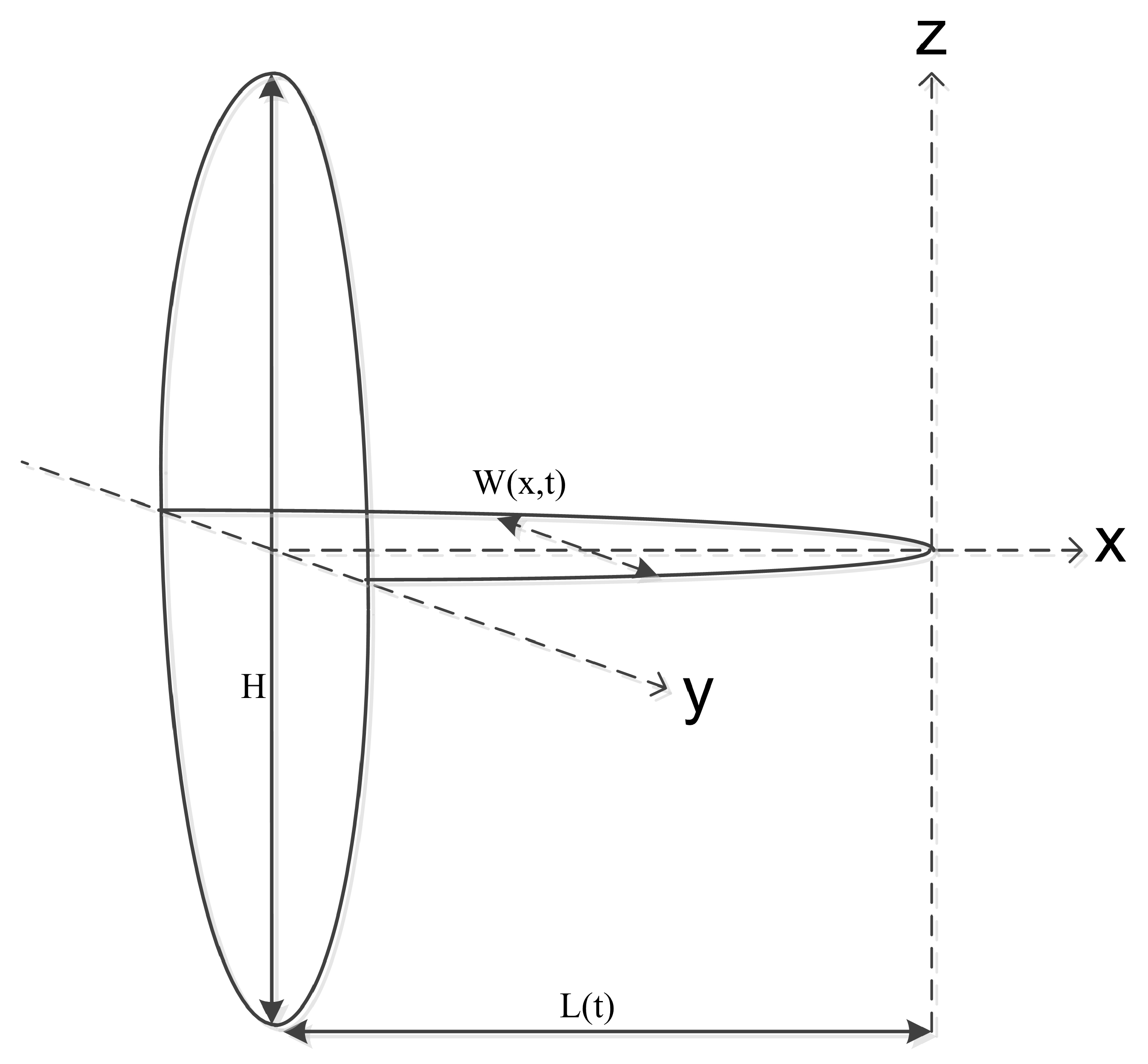
3.1. Dynamic Modeling of Hydraulic Fracturing

In this work, a large-scale process model of hydraulic fracturing is developed by adopting the following assumptions: (1) fracture propagation is described by Perkins, Kern, and Nordgren (PKN) model as shown in Figure 1 [26]; (2) the layers above and below have sufficiently large stresses such that the vertical fracture is confined within a single horizontal rock layer; (3) the fracture length is much greater than fracture width; (4) the fluid pressure is constant in the vertical direction; and (5) the fracture is surrounded by an isotropic homogenous elastic material.

The dynamic modeling of hydraulic fracturing involves two sub-processes: fracture propagation and proppant transport. A brief description of the governing equations is presented below. The fluid flow rate in the horizontal direction is determined by the following equation for flow of a Newtonian fluid in an elliptical section [2,27]:

$$\frac{dP}{dx}=-\frac{64\mu Q}{\pi H{W}^3}$$

(7)

where P is the net pressure, $x\in [0,L(t\left)\right]$ is the time-dependent spatial coordinate in the horizontal direction, $\mu$ is the fluid viscosity, Q is the fluid flow rate in the horizontal direction, H is the predefined fracture height, and W is the fracture width.

For a crack under constant normal pressure, the fracture shape is elliptical as shown in Figure 1. The relationship between the maximum fracture width (i.e., the minor axis of the ellipse) and the net pressure is given as follows [28,29]:

$$W=\frac{2PH(1-{\nu }^2)}{E}$$

(8)

where $\nu$ is the Poisson ratio of the formation, and E is the Young’s modulus of the formation.

By taking into account the fracture volume changes and the fluid leak-off into the reservoir, the continuity equation for an incompressible fluid flow inside the fracture is given by [27]:

$$\frac{\partial A}{\partial t}+\frac{\partial Q}{\partial x}+HU=0$$

(9)

where $A=\pi WH/4$ is the cross-sectional area of the elliptic fracture, and U is the fluid leak-off per unit height accounting for both fracture walls, which is determined by the following expression [2,30]:

$$U=\frac{2C_{leak}}{\sqrt{t-\tau \left(x\right)}}$$

(10)

where $C_{leak}$ is the overall leak-off coefficient, t is the elapsed time since fracturing was initiated, and $\tau \left(x\right)$ is the time at which the fracture propagation has arrived at x for the first time.

Plugging Equations (7) and (8) into Equation (9) results in the following nonlinear parabolic PDE:

$$\frac{\pi H}{4}\frac{\partial W}{\partial t}-\frac{\pi E}{128\mu (1-{\nu }^2)}\left[3W^2{\left(\frac{\partial W}{\partial x}\right)}^2+W^3\frac{{\partial }^{2}W}{\partial x^2}\right]+HU=0$$

(11)

The initial condition for solving the above equations is that the fracture is closed, that is $W(x,0)=0$. In addition, the two boundary conditions are considered as follows:

• At the wellbore, the fluid flow rate is specified by $Q(x,t)=Q_0\left(t\right)$, where $Q_0\left(t\right)$ is the fluid injection rate (i.e., the manipulated variable).
• At the fracture tip, $x=L\left(t\right)$, the fracture is always closed, that is $W\left(L\right(t),t)=0$.

The modeling of the injected proppant transport is based on the following assumptions: (1) along the horizontal direction, the injected proppant will travel at the fracturing fluid’s velocity; (2) the suspended proppant will settle towards the fracture bottom due to the gravitational force which will lead to the formation of a proppant bank; (3) proppant particles are sufficiently large so that the diffusive flux can be neglected when the convective flux is considered; and (4) because of low proppant concentration, the interactions between the individual particles are neglected, while the drag and gravitational forces acting on the proppant particles are still considered. Based on these assumptions, the advection of the suspended proppant can be expressed by the following equation:

$$\frac{\partial \left(WC\right)}{\partial t}+\nabla ·\left(WC{V}_p\right)=0$$

(12)

$$C(0,t)=C_0\left(t\right)\mathrm{and}C(x,0)=0$$

(13)

where C is the suspended proppant concentration, ∇ is the vector differential operator, $V_p$ is the velocity with which the proppant particles are advected, and $C_0\left(t\right)$ is the inlet proppant concentration at the wellbore (i.e., the manipulated variable).

The net velocity of the proppant particles, $V_p$, is dependent on the suspended proppant concentration, C, the fluid velocity, V, and the gravitational settling velocity, $V_s$, which is given by the following expression [31]:

$$V_p=V-(1-C)V_s$$

(14)

The gravity-induced proppant settling velocity in the fracturing fluid, $V_s$, is computed as follows [32]:

$$V_s=\frac{{(1-C)}^2}{{10}^{1.82C}}\frac{({\rho }_{sd}-{\rho }_f)g{d}^2}{18\mu }$$

(15)

where ${\rho }_{sd}$ is the proppant particle density, ${\rho }_f$ is the pure fluid density, g is the gravitational acceleration constant, d is the proppant diameter, and $\mu$ is the fracture fluid viscosity where its relation with the proppant concentration can be described by the following empirical model [33]:

$$\mu \left(C\right)={\mu }_0{\left(1-\frac{C}{C_{max}}\right)}^{-\beta }$$

(16)

where ${\mu }_0$ is the pure fluid viscosity, $\beta$ is an exponent in the range of 1.2 to 1.8, and $C_{max}$ is the theoretical maximum proppant concentration determined by $C_{max}=(1-\varphi ){\rho }_{sd}$ where $\varphi$ is the proppant bank porosity. The particles settle out of the flow to the fracture bottom and form a proppant bank. The evolution of proppant bank height, $\delta$, via the proppant settling is given as follows [34,35]:

$$(1-\varphi )\frac{d\left(\delta W\right)}{dt}=C{V}_{s}W$$

(17)

where proppant bank is initially of vanishing thickness, so the initial condition is that $\delta (x,0)=0$.

The above-mentioned PDE-ODE systems defined over time-dependent spatial domains will be solved using an in-house simulator developed by Siddhamshetty et al. [8].

3.2. Obtaining Cost-to-Go Function Offline

3.2.1. Simulation of Sub-Optimal Control Policies for ADP

In this section, a nonlinear MPC formulation is presented to obtain sub-optimal control policies for ADP. First, we employed unified fracture design (UFD) technique to obtain the optimal fracture length ($L_{opt}$) and width ($W_{opt}$) for a specific amount of proppant, $M_{prop}$, to be injected into a reservoir well [36]. Additionally, the target proppant concentration, $C_{target}$, at the end of hydraulic fracturing is calculated as follows:

$$C_{target}=\frac{M_{prop}}{H{L}_{opt}{W}_{opt}}$$

(18)

The high-fidelity process model described in Equations (7)–(17) demands high computational requirements, and thus, it cannot be directly employed for the controller design. While there are a variety of computationally efficient linear [11,37,38] and nonnlinear [10,39,40,41,42] MOR techniques available, in this work, we developed a reduced-order model (ROM) based on multivariate output error state space (MOESP) algorithm using the simulation results from the high-fidelity model as described in [8]. The developed ROM is presented as follows:

$$\begin{array}{c}x\left(t_{k+1}\right)=Ax\left(t_k\right)+Bu\left(t_k\right)\hfill \end{array}$$

(19a)

$$\begin{array}{c}y\left(t_k\right)=Hx\left(t_k\right)\hfill \end{array}$$

(19b)

where $x\left(t_k\right)$ represents the vector of states in the state space model at time instant $t_k$, A, B and H represent the system matrices, $y\left(t_k\right)={[W_0\left(t_k\right),L\left(t_k\right),C(x_1,t_k),C(x_2,t_k),C(x_3,t_k),C(x_4,t_k),C(x_5,t_k),C(x_6,t_k)]}^T$ represents the vector of output variables, $W_0\left(t_k\right)$ is the fracture width at the wellbore, $L\left(t_k\right)$ is the fracture length, $C(x_1,t_k),\cdots ,C(x_6,t_k)$ are the proppant concentrations at six different locations across the fracture, and $u\left(t_k\right)={[C_0\left(t_k\right),C_0(t_k-{\zeta }_{x_1}),C_0(t_k-{\zeta }_{x_2}),C_0(t_k-{\zeta }_{x_3}),C_0(t_k-{\zeta }_{x_4}),C_0(t_k-{\zeta }_{x_5}),C_0(t_k-{\zeta }_{x_6})]}^T$ is the inlet proppant concentration at the wellbore (i.e., the manipulated input variable), ${\zeta }_{x_i}$ is the input time-delay due to the time required for the proppant to travel from the wellbore to a particular location $x_i$.

Remark 1.

Please note the linear discrete-time state space model is good for the purpose of this study. To develop the ROM, we varied the input profile so that we can cover the entire range of operating conditions that are being considered in the oil reservoir field. Alternatively, a nonlinear ROM can be used to improve the controller performance as the governing equation is indeed a nonlinear parabolic PDE with the moving boundary.

In hydraulic fracturing, the readily available real-time measurements are limited to the fracture length and the fracture width at the wellbore, which are provided via the processed microseismic and downhole pressure data, respectively [43]. To estimate the remaining important state variables such as the proppant concentration across the fracture, we designed a Kalman filter by adding the process and measurement noise to the ROM presented in Equation (19) as described in [8]:

$$\begin{array}{c}x\left(t_{k+1}\right)=Ax\left(t_k\right)+Bu(t_k-\zeta )+v\left(t_k\right)\hfill \end{array}$$

(20a)

$$\begin{array}{c}y\left(t_k\right)=Hx\left(t_k\right)+w\left(t_k\right)\hfill \end{array}$$

(20b)

where v denotes the process noise, and w denotes the measurement noise. The process noise is assumed to be drawn from a zero mean multivariate normal distribution with covariance Q, and the measurement noise is assumed to be zero mean Gaussian white noise with covariance R.

The state estimator algorithm works in a two-step process: prediction and measurement update. Combining these two steps, the Kalman filter equations can be written as follows:

$$\begin{array}{c}\widehat{x}\left(t_{k+1}\right)=A\widehat{x}\left(t_k\right)+Bu(t_k-\zeta )+M\left(t_k\right)(y_m\left(t_k\right)-\widehat{y}\left(t_k\right))\hfill \end{array}$$

(21a)

$$\begin{array}{c}M\left(t_k\right)=P\left(t_k\right)H^T{(R\left(t_k\right)+HP\left(t_k\right)H^T)}^{-1}\hfill \end{array}$$

(21b)

$$\begin{array}{c}P\left(t_{k+1}\right)=(I-M\left(t_k\right)H)P\left(t_k\right)\hfill \end{array}$$

(21c)

where the operator $\widehat{(·)}$ is used to denote the estimated variables, $M\left(t_k\right)$ is the Kalman filter gain, and $P\left(t_k\right)$ denotes the covariance of the state estimation error.

To determine sub-optimal control policies for ADP, we employed the following MPC scheme designed by Siddhamshetty et al. [8]:

$$\begin{array}{c}\underset{C_{stage,k}}{min}{(\mathbf{C}\left(t_f\right)-C_{target}\mathbb{1})}^T{Q}_c(\mathbf{C}\left(t_f\right)-C_{target}\mathbb{1})\hfill \end{array}$$

(22a)

$$\begin{array}{c}\mathrm{s}.\mathrm{t}.\mathrm{ROM},\mathrm{Equation}\left(19\right)\hfill \end{array}$$

(22b)

$$\begin{array}{c}\mathrm{Kalman}\mathrm{filter},\mathrm{Equation}\left(19\right)\hfill \end{array}$$

(22c)

$$\begin{array}{c}{C}_{min}\mathbb{1}\le \mathbf{C}(t_k+j\Delta )\le C_{max}\mathbb{1},\forall j=0,\cdots ,10-k\hfill \end{array}$$

(22d)

$$\begin{array}{c}{C}_{stage,k-1+m}\le C_{stage,k+m}\le C_{stage,k-1+m}+4\left(\mathrm{ppga}\right),m=1,\cdots ,10-k\hfill \end{array}$$

(22e)

$$\begin{array}{c}2Q_0\Delta \left(\sum _k{C}_{stage,k}\right)=M_{prop}\hfill \end{array}$$

(22f)

$$\begin{array}{c}L\left(t_f\right)=L_{opt},W_0\left(t_f\right)\ge W_{opt}\hfill \end{array}$$

(22g)

where $t_f$ denotes the total treatment time, $Q_c$ is a positive definite matrix used to compute the weighted norm, $t_k$ is the current time, $\Delta$ is the time interval between sampling times, $\mathbf{C}\left(t_k\right)={[C_1\left(t_k\right),C_2\left(t_k\right),C_3\left(t_k\right),C_4\left(t_k\right),C_5\left(t_k\right),C_6\left(t_k\right)]}^T$ is the proppant concentration inside the fracture at six different locations at $t=t_k$, $\mathbb{1}$ is a $6\times 1$ vector whose elements are all ones, $W_0\left(t_k\right)$ and $L\left(t_k\right)$ are the only readily available real-time measurements of the fracture width at the wellbore and the fracture length at $t=t_k$, respectively, and $C_{stage,k}$ is the inlet proppant concentration (i.e., the manipulated input) corresponding to the $k^{th}$ time interval i.e., $t\in [t_k,t_{k+1})$, which can be computed by solving Equation (22) with a shrinking prediction horizon $N_p=t_f-t_k$.

In the above optimization problem, the penalty function, Equation (22a), computes the squared deviation of the proppant concentration from the set-point at 6 different locations across the fracture at the end of pumping. At every sampling time $t_k$, the Kalman filter of Equation (21) is initialized to estimate the proppant concentration $\widehat{\mathbf{C}}$ by using the real-time measurements of the fracture width at the wellbore and the fracture length. The constraint of Equation (22d) imposes limits on the concentration profiles to avoid premature termination of the hydraulic fracturing process. The constraint of Equation (22e) demands a monotonic increase in the input proppant concentration with an increment less than 4 ppga/stage, where ppga is a concentration unit used in petroleum engineering that refers to one pound of proppant added to a gallon of water. The constraint of Equation (22f) specifies the total amount of proppant to be injected. The terminal constraint of Equation (22g) employs the optimal fracture geometry, which is calculated by UFD scheme described in the preceding paragraph.

The dynamic model described in Section 3.1 was utilized to simulate the hydraulic fracturing process using the parameters listed in

Table 1. Model parameters used for the simulation.

Parameter	Symbol	Value
Leak-off coefficient	$C_{leak}$	6.3 × ${10}^{-5}$m/s${}^{1/2}$
Maximum concentration	$C_{max}$	0.64
Minimum concentration	$C_{min}$	0
Young’s modulus	E	0.5 × ${10}^{10}$ Pa
Proppant permeability	$k_f$	60,000 mD
Formation permeability	$k_r$	1.5 mD
Vertical fracture height	H	20 m
Proppant particle density	${\rho }_{sd}$	2648 kg/m${}^3$
Pure fluid density	${\rho }_f$	1000 kg/m${}^3$
Fracture fluid viscosity	$\mu$	0.56 Pa·s
Poisson ratio of formation	$\nu$	0.2

. In hydraulic fracturing, the characterization of rock mechanical properties is one of the key tasks that has to be performed prior to the model based controller design. This requires the availability of field data. Currently, in the field, a small-scale experiment called the mini-frac test is performed to collect preliminary data that can be used to characterize the geological properties. However, in this work, the model parameters utilized to simulate the hydraulic fracturing process are taken from literature [8,44]. Specifically, we considered 48,000 kg of proppant amount to be injected during the entire hydraulic fracturing process. For this fixed amount of proppant, we employed UFD scheme to obtain the corresponding optimal fracture length $L_{opt}=135$ m and width $W_{opt}=5.4$ mm, which were used as the optimal fracture geometry constraint (Equation (22g)) in the MPC formulation that has to be satisfied at the end of pumping. Then, the target proppant concentration at the end of pumping, $C_{target}=9.765$ ppga, was calculated using Equation (18). The positive definite matrix, $Q_c$, was considered to be a diagonal matrix with the diagonal entries equal to 100. The pad time, $t_p$, was fixed to be 220 s and the constant flow rate of $Q_0=0.03$ m${}^3$/s was used after the pad time. The Kalman filter and feedback control systems were initialized at the end of pad time (i.e., $t_k\ge t_p$). In the closed-loop simulation, $t_f$ and $\Delta$ were chosen to be 1220 s and 100 s, respectively. The proppant pumping schedule was divided into 10 substages and the duration of each substage was identical to $\Delta$. At each sampling time, the controller was called and the first input, $C_{stage,k}$, of the entire input profile ($C_{stage,k},C_{stage,k+1},\cdots$) obtained by solving the optimization problem over a prediction horizon length of $N_p$ was applied to the dynamic model in a sample-and-hold fashion, and this procedure was repeated at each sampling time until the end of treatment. Please note that the controller performance can be improved by increasing the number of proppant pumping substages while maintaining the number of spatial locations across the fracture, at which we want to achieve the uniform proppant concentration [8]. However, it is not viable to have a large number of substages, and hence, we selected 10 substages because we did not observe significant improvement after that.

Remark 2.

Please note that Kalman filter is applied before the MPC optimization. Specifically, at every sampling time $t_k$, the real-time measurements of the fracture width at the wellbore, $W_0\left(t_k\right)$, and the fracture length, $L\left(t_k\right)$, were obtained from the high-fidelity model, which is a virtual experiment. These measurements were then utilized by Kalman filter of Equation (21) to estimate the (unmeasurable) proppant concentration inside the fracture at $t=t_k$. Finally, the inlet proppant concentration (i.e., the manipulated input), $C_{stage,k}$, was obtained by solving the optimization problem with the cost function of Equation (22a) under the constraints described by Equations (22b) and (22d)–(22g).

The data covering the relevant regions in the continuous state space was obtained from the closed-loop simulations under the above-mentioned MPC scheme by initializing the Kalman filter and the feedback control systems with different fracture width at the wellbore and fracture length values at $t=t_p$, which were obtained by varying the flow rate $Q_0$ during the pad time—i.e., $t\in [0,t_p)$. In this work, the pad time $t_p$ was fixed, and therefore, the fracture width at the wellbore and the fracture length at the end of pad time depended only on the flow rate $Q_0$. Every different $Q_0$ profile during the pad time would result in a unique combination of the fracture width at the wellbore and the fracture length at the end of pad time that allows the feedback system to compute a control input profile, which is dissimilar to other profiles, if their $Q_0$ during the pad time is different. In each closed-loop simulation, the real-time measurements of the fracture width at the wellbore and the fracture length were taken at 10 time instants (i.e., 10 substages). At each time instant, the real-time measurement was utilized by the Kalman filter to estimate the (unmeasurable) proppant concentration inside the fracture. Each measurement can be represented as $y\left(t_k\right)={[W_0\left(t_k\right),L\left(t_k\right)]}^T$ and the corresponding estimated state can be represented as $\widehat{\mathbf{C}}\left(t_k\right)={[{\widehat{C}}_1\left(t_k\right),{\widehat{C}}_2\left(t_k\right),{\widehat{C}}_3\left(t_k\right),{\widehat{C}}_4\left(t_k\right),{\widehat{C}}_5\left(t_k\right),{\widehat{C}}_6\left(t_k\right)]}^T$ where ${\widehat{C}}_i\left(t_k\right)$ is the proppant concentration inside the fracture at a specific location i at $t=t_k$. Twenty-four closed-loop simulations were performed by initializing the Kalman filter and the feedback control systems with 24 different initial conditions, resulting in 240 real-time measurements (denoted by $X_{measure}$) and the corresponding set of 240 estimated states (denoted by $X_{est}$).

Remark 3.

In hydraulic fracturing, the real-time measurement of the proppant concentration inside the fracture is not available due to the remote subterranean location where the fracture propagates. To overcome this challenge, we used the Kalman filter to estimate the proppant concentration based on the available real-time measurements of the fracture width at the wellbore and the fracture length. Therefore, we use the term “estimated states” in Section 3 instead of “sampled states” as described in Section 2.

3.2.2. Initial Cost-to-Go Approximation

For all of the estimated states during the closed-loop simulations, the initial cost-to-go values ($J^{{\mu }^0}$) were computed as follows:

$$J^{{\mu }^0}(\widehat{\mathbf{C}}\left(t_k\right))=\sum _{j=k}^{N_t}\Phi (\widehat{\mathbf{C}}\left(t_j\right),u\left(t_j\right))$$

(23)

where $N_t=10$ is the number of time instants where the proppant concentrations are estimated by the Kalman filter during each closed-loop simulation, and $\Phi (\widehat{\mathbf{C}}(t_j),u\left(t_j\right))$ is given by the following equation:

$$\Phi (\widehat{\mathbf{C}}\left(t_j\right),u\left(t_j\right))={(\widehat{\mathbf{C}}\left(t_{j+1}\right)-C_{target}\mathbb{1})}^T{Q}_c(\widehat{\mathbf{C}}\left(t_{j+1}\right)-C_{target}\mathbb{1})$$

(24)

A function approximator, denoted as ${\tilde{J}}^{{\mu }^0}(\widehat{\mathbf{C}})$, was constructed to obtain the mapping between initial cost-to-go values and the estimated states (i.e., proppant concentration $\widehat{\mathbf{C}}$) obtained during the closed-loop simulations. We used KNN (with $K=5$) as a function approximator. In hydraulic fracturing, the real-time measurements readily available are limited to the fracture width at the wellbore and the fracture length. Therefore, we used only these two available measurements to determine the KNN. The function approximator works in the following way. Suppose there is a new measurement y. First, we determine the KNN of y from the set $X_{measure}$, which consists of 240 real-time measurements obtained during the closed-loop simulations. Let the KNN of y be $y_1,y_2,\cdots ,y_K$ with the Euclidean distances $d_1,d_2,\cdots ,d_K$, respectively, from y. Second, we select K proppant concentration vectors ${\widehat{\mathbf{C}}}_1,{\widehat{\mathbf{C}}}_2,\cdots ,{\widehat{\mathbf{C}}}_K$ from $X_{est}$ which were estimated by the Kalman filter utilizing $y_1,y_2,\cdots ,y_K$ during the closed-loop simulations, respectively. Then, the selected K proppant concentration vectors ${\widehat{\mathbf{C}}}_1,{\widehat{\mathbf{C}}}_2,\cdots ,{\widehat{\mathbf{C}}}_K$ are used in Equation (25) to determine the cost-to-go at a new state $\widehat{\mathbf{C}}$ estimated by the Kalman filter utilizing the new measurement y.

$$\tilde{J}\left(\widehat{\mathbf{C}}\right)=\sum _{j=1}^K{w}_j\tilde{J}\left({\widehat{\mathbf{C}}}_j\right)$$

(25)

where

$$w_j=\frac{1/d_j}{{\sum }_{i=1}^{K}1/d_i}$$

(26)

The schematic diagram of the above procedure is shown in Figure 2.

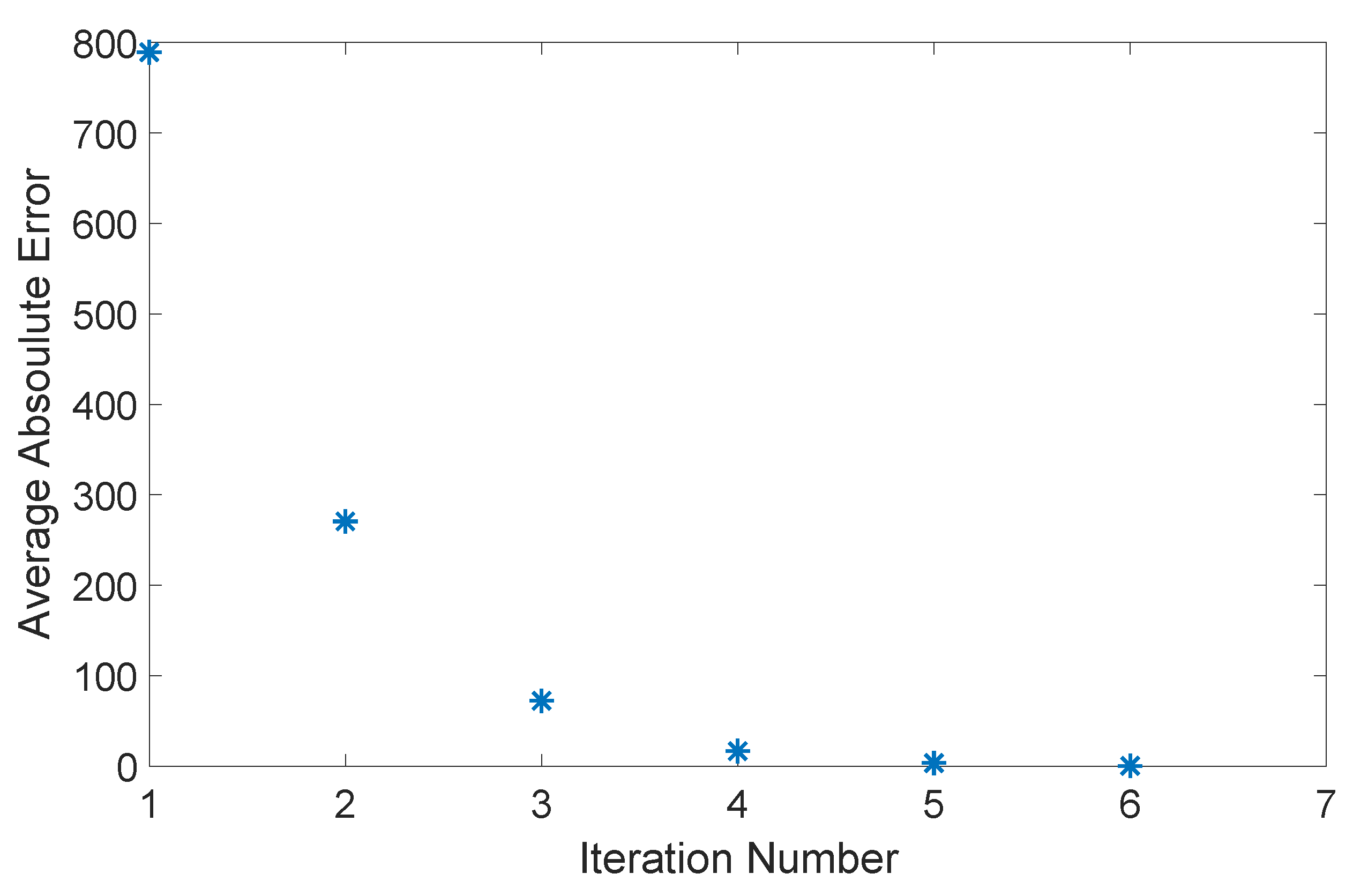
3.2.3. Bellman Iteration

Value iteration is employed for offline cost-to-go improvement. In this approach, Bellman equation (Equation (3)) is solved iteratively for every estimated state in $X_{est}$ until convergence. At each iteration step, we calculate $J^{i+1}$ for every estimated state $\widehat{\mathbf{C}}\left(t_k\right)$ by solving:

$$J^{i+1}\left(\widehat{\mathbf{C}}\left(t_k\right)\right)=\underset{u\left(t_k\right)\in \mathcal{U}}{min}[\Phi (\widehat{\mathbf{C}}\left(t_k\right),u\left(t_k\right))+{\tilde{J}}^i\left(\widehat{\mathbf{C}}\left(t_{k+1}\right)\right)]$$

(27)

where the superscript i denotes the iteration index, $J^{i+1}$ is the updated cost-to-go value for $\widehat{\mathbf{C}}\left(t_k\right)$, ${\tilde{J}}^i\left(\widehat{\mathbf{C}}\left(t_{k+1}\right)\right)$ is the estimate of cost-to-go value for the successor state $\widehat{\mathbf{C}}\left(t_{k+1}\right)$ and ${\tilde{J}}^0={\tilde{J}}^{{\mu }^0}$. After updating the cost-to-go values for all of the estimated states in $X_{est}$, we fit another function approximator to the resulting $\widehat{\mathbf{C}}$ vs. $J^{i+1}(\widehat{\mathbf{C}})$ data.

In this work, the Bellman iterations converged after six iterations with the following termination condition:

$$\frac{1}{N}\sum _{k=1}^N|J^{i+1}\left(x_k\right)-J^i\left(x_k\right)|<0.35$$

(28)

where $N=240$ is the total number of estimated states during the closed-loop simulations. Figure 3 shows how the average absolute error, $\frac{1}{N}{\sum }_{k=1}^N|J^{i+1}\left(x_k\right)-J^i\left(x_k\right)|$, changes in subsequent iterations. In ADP, the time evolution of the system states is described by employing the ROM, developed for the MPC scheme, because of the high computational effort required to solve the high-fidelity model.

Remark 4.

In the ADP approach, the data covering the relevant regions in the continuous state space can be obtained by performing closed-loop simulations of the system under any known heuristics or sub-optimal control policies. The initial cost-to-go estimates do not affect the quality of the converged cost-to-go function [45,46]. Therefore, the performance of the ADP-based controller does not heavily rely on the MPC design. In this work, we employed the MPC scheme developed by Siddhamshetty et al. [8] because it provides a good input profile compared to other available input profiles such as Nolte’s pumping schedule.

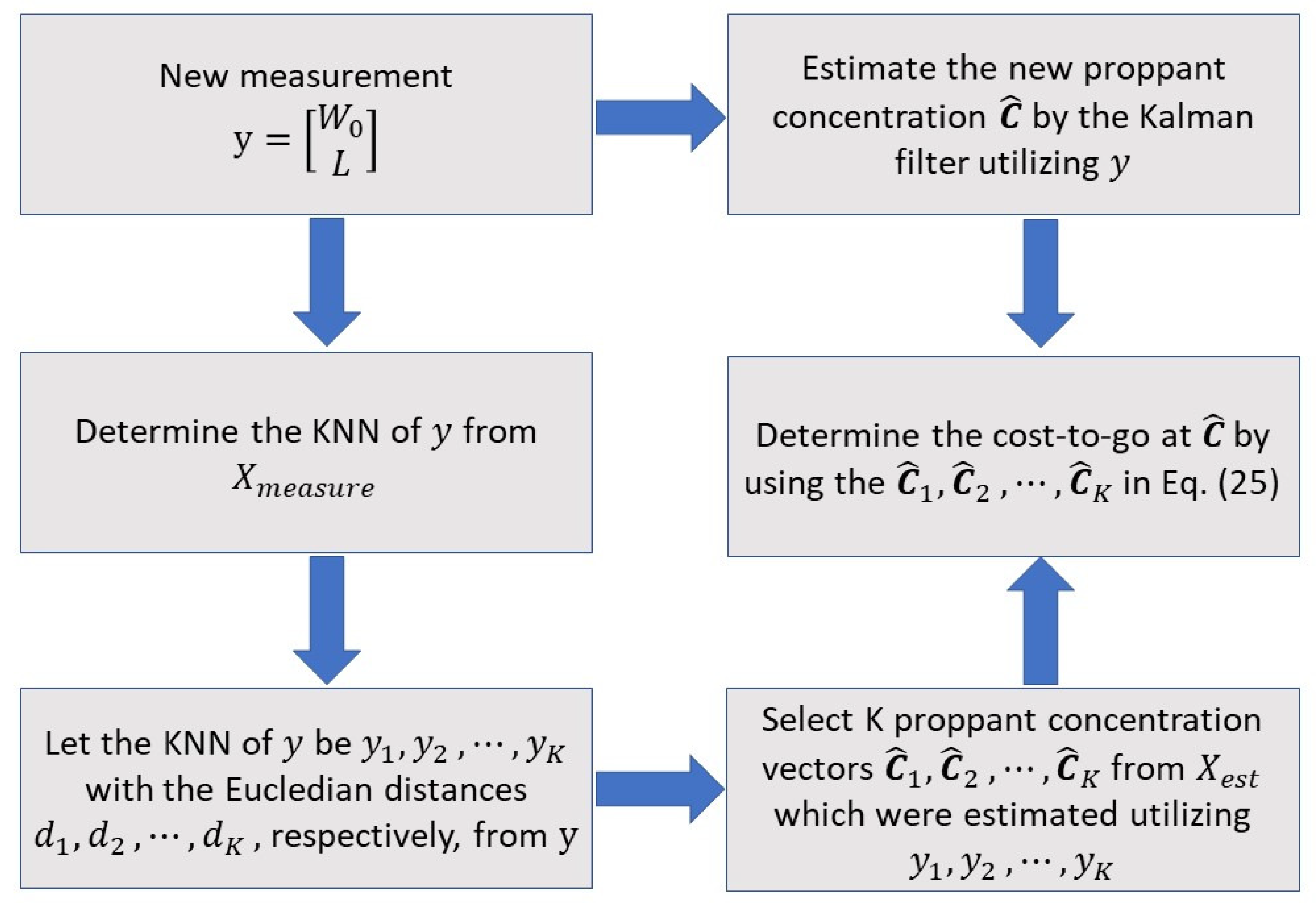
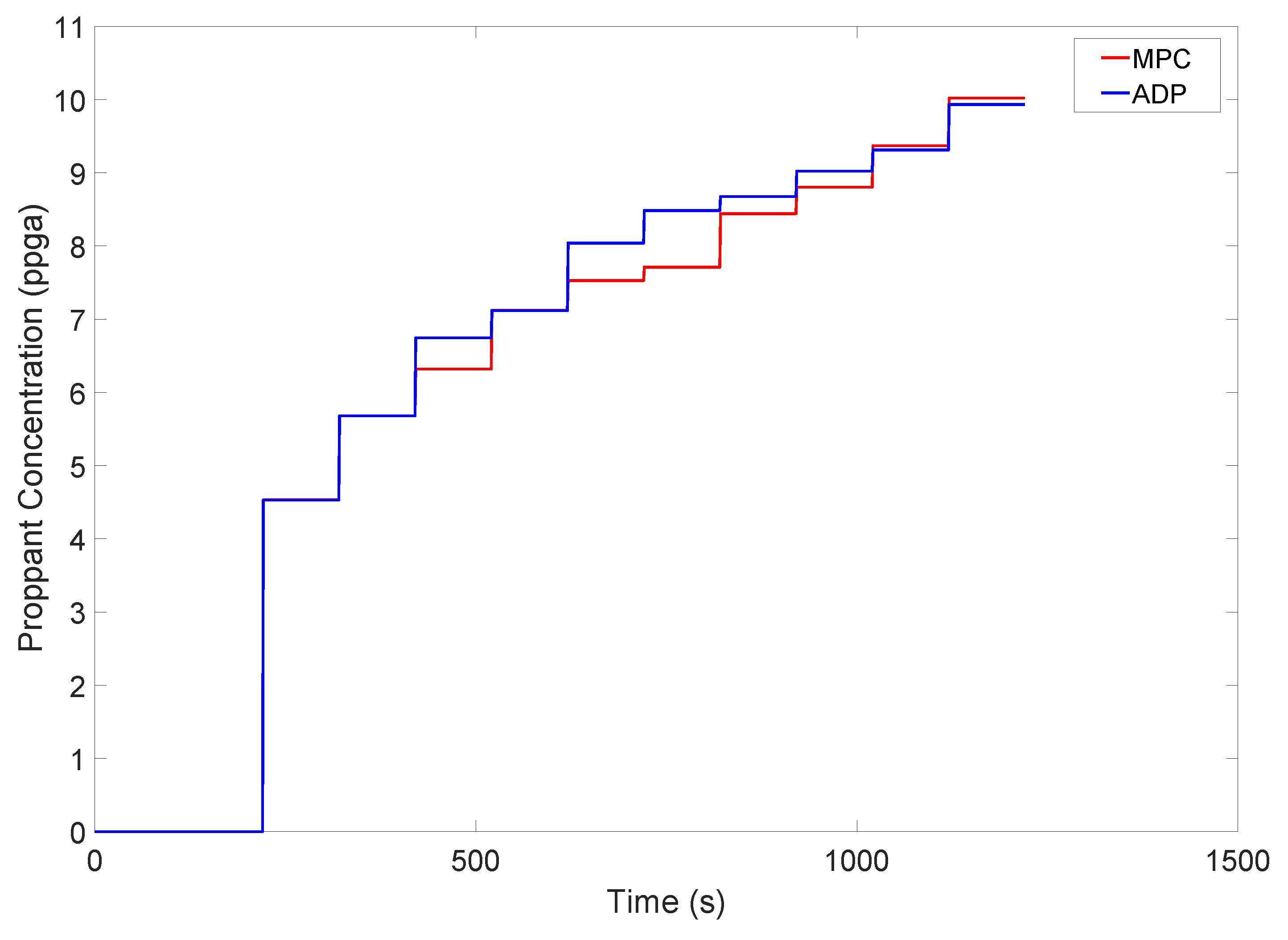
3.3. Online Optimal Control

Once the cost-to-go iteration converges, we compute the control policy online by solving the following optimization problem:

$$u\left(t_k\right)=\arg \underset{u\left(t_k\right)\in \mathcal{U}}{min}[\Phi (\widehat{\mathbf{C}}\left(t_k\right),u\left(t_k\right))+{\tilde{J}}^{N_c}(\widehat{\mathbf{C}}\left(t_{k+1}\right))]$$

(29)

where $N_c=6$ represents the number of iterations required for convergence, and ${\tilde{J}}^{N_c}$ denotes the converged cost-to-go function approximator.

The ADP-based controller is employed to achieve the uniform proppant concentration across the fracture at the end of pumping. To compare the performance of the ADP-based controller with the MPC system, we perform the closed-loop simulations under both of the control systems by initializing the Kalman filter with the fracture width at the wellbore and the fracture length values outside the “training set”. We want to note that the “training set” refers to the set of values of the fracture width at the wellbore and the fracture length used to initialize the Kalman filter during the closed-loop simulations under the MPC system as described in Section 3.2.1. The profiles of the injected proppant concentration at the wellbore (i.e., the manipulated input) and proppant concentration across the fracture at the end of pumping using ADP-based controller and the MPC system are shown in Figure 4 and Figure 5. The ADP-based controller shows an improvement over the MPC system in achieving the uniform proppant concentration across the fracture at the end of pumping. The performance of the closed-loop response can be understood based on the total cost-to-go values. Specifically, the cost-to-go values for the ADP-based controller and the MPC system are $179.66\times {10}^3$ and $181.58\times {10}^3$, respectively. Furthermore, the ADP-based controller takes less computational time than the MPC system to run a closed-loop simulation as shown in Figure 6. This is because ADP-based controller solves a single-stage optimization problem, Equation (29), whereas the MPC system solves a multi-stage optimization problem, Equation (22), at each sampling time. In MPC, the computational time required to solve the optimization problem keeps decreasing with time because the number of remaining stages to be considered keeps decreasing. However, in ADP, the computational time required at each sampling time is similar because ADP solves a single-stage optimization problem at every sampling time. Please note that the calculations were performed on a Dell workstation, powered by Intel(R) Core(TM) i74770 [email protected] GHz, running the Windows 8 operating system. We would like to highlight that the reduction in the computational time can be very beneficial to enhance the productivity of the produced wells. Specifically, despite advances in measurement techniques, it still requires interruption by experienced engineers to distinguish useful information from noise. For example, it takes about 1–3 min to post-process the microseismic data. Therefore, having a computationally efficient controller such as ADP-based controllers would compensate for the time delay due to the interruption by experienced engineers.

Remark 5.

In the ADP-based controller, we did not include the constraints directly but used the data from 24 closed-loop simulations which satisfied the constraints. Specifically, for every sampling time $t_k$, we stored 24 values of the manipulated input obtained from the 24 closed-loop simulations. Let $C_k^{LB}$ and $C_k^{UB}$ be the minimum and the maximum value of the manipulated input at time instant $t_k$ among the 24 stored values, respectively. Finally, at every sampling time $t_k$, Equations (27) and (29) were solved with $C_k^{LB}$ and $C_k^{UB}$ as the lower and the upper bound, respectively.

3.4. ADP-Based Control with Plant–Model Mismatch

We also studied the performance of the ADP-based controller when the rock mechanical properties are not available a priori. Specifically, we considered a plant–model mismatch in Young’s modulus, E, which significantly affects the controller performance with respect to achieving uniform proppant concentration across the fracture at the end of pumping [44,47].

In this case, the data covering the relevant regions in the state space was obtained from the closed-loop simulations under the MPC system described in Section 3.2.1 by considering the following five different scenarios: (1) no variation in E; (2) 15% increase in E; (3) 5% increase in E; (4) 5% decrease in E; and (5) 15% decrease in E. For each value of E, a total of five closed-loop simulations under the MPC system of Equation (22) were performed by initializing the Kalman filter with different values of the fracture width at the wellbore and the fracture length. As a result, a total of 250 estimated states were obtained from the five scenarios. For all the estimated states, the initial cost-to-go values ($J^{{\mu }^0}$) were computed using Equation (23). Then, we employed KNN (with $K=5$) as a function approximator to obtain the mapping between initial cost-to-go values and the estimated states as described in Section 3.2.2. This was followed by the value iteration step in which the Bellman iterations converged after five iterations with the following termination condition:

$$\frac{1}{N}\sum _{k=1}^N|J^{i+1}\left(x_k\right)-J^i\left(x_k\right)|<0.35$$

(30)

where $N=250$ is the total number of estimated states obtained from the five scenarios. Figure 7 shows how the average absolute error, $\frac{1}{N}{\sum }_{k=1}^N|J^{i+1}\left(x_k\right)-J^i\left(x_k\right)|$, changes in subsequent iterations. Please note that the ROM used to run the closed-loop simulations under the MPC system for five different scenarios is developed with a fixed E, which is $0.5\times {10}^{10}$ Pa (i.e., no variation in E). Therefore, it does not capture the plant–model mismatch due to uncertainty in E. In this work, the same ROM with a fixed E is used in the ADP-based controller to demonstrate its capability of handling a plant–model mismatch in E.

To test the performance of the ADP-based controller, we performed the closed-loop simulation with the converged cost-to-go function by considering 10% decrease in E and by initializing the Kalman filter with the fracture width at the wellbore and the fracture length values outside the “training set”. Note that the “training set” refers to the set of values of the fracture width at the wellbore and the fracture length used to initialize the Kalman filter during the closed-loop simulations under the MPC system for five scenarios. The profiles of the injected proppant concentration at the wellbore (i.e., the manipulated input) and proppant concentration across the fracture at the end of pumping using the ADP-based controller are shown in Figure 8 and Figure 9. It can be observed in Figure 9 that the ADP-based controller is able to achieve uniform proppant concentration across the fracture at the end of pumping. In other words, it effectively handled the plant–model mismatch in E. Please note that, even with the same rock formation, the performance of hydraulic fracturing can be significantly different [48,49]. This variability can, in part, be attributed to the spatially varying rock mechanical properties such as the Young’s modulus, E. Therefore, having a controller such as the ADP-based control framework that can handle the plant–model mismatch in E can play a crucial role in enhancing the productivity of the produced well.

Remark 6.

Please note that in robust MPC-based methods [50,51,52,53], model parameter uncertainty has been directly considered in designing MPC. However, in the proposed ADP-based controller, the uncertainty in the model parameter (i.e., Young’s modulus, E) is handled by developing an accurate cost-to-go function during the offline stage.

4. Conclusions

In this work, we developed an ADP-based strategy to regulate the proppant concentration across the fracture at the end of pumping in hydraulic fracturing. First, we performed the closed-loop simulations under the standard MPC to obtain measurable outputs, which were then used to estimate unmeasurable states by the Kalman filter, and to initialize the cost-to-go function approximation in ADP. Second, we employed the value iteration for the cost-to-go improvement by performing iterations of the Bellman equation for all the estimated states during the closed-loop simulations under the standard MPC. Lastly, the ADP-based controller with the converged cost-to-go function approximator was employed for the design of a feedback control system to achieve uniform proppant concentration across the fracture at the end of pumping. The generated pumping schedule using the proposed ADP-based control framework was able to produce a uniform proppant concentration that was closer to the target concentration than the pumping schedule generated by the standard MPC. The ADP-based controller was able to generate an online pumping schedule at a fraction of the time required for the standard MPC as we only had to solve the single-stage optimization problem at each sampling time. Furthermore, the ADP-based controller was able to handle the plant–model mismatch in the Young’s modulus of a rock formation. Therefore, this method holds promise to control the hydraulic fracturing process by handling uncertainties in the important geological properties.

References

1. Economides, M.J.; Watters, L.T.; Dunn-Normall, S. Petroleum Well Construction; Wiley: New York, NY, USA, 1998. [Google Scholar]
2. Economides, M.J.; Nolte, K.G. Reservoir Stimulation; John Wiley & Sons: New York, NY, USA, 2000. [Google Scholar]
3. Economides, M.J.; Martin, T. Modern Fracturing: Enhancing Natural Gas Production; ET Publishing: Houston, TX, USA, 2007. [Google Scholar]
4. Nolte, K.G. Determination of proppant and fluid schedules from fracturing-pressure decline. SPE Prod. Eng. 1986, 1, 255–265. [Google Scholar] [CrossRef]
5. Gu, H.; Desroches, J. New pump schedule generator for hydraulic fracturing treatment design. In Proceedings of the SPE Latin American and Caribbean Petroleum Engineering Conference, Port-of-Spain, Trinidad and Tobago, 27–30 April 2003. [Google Scholar]
6. Dontsov, E.V.; Peirce, A.P. A new technique for proppant schedule design. Hydraul. Fract. J. 2014, 1, 1–8. [Google Scholar]
7. Gu, Q.; Hoo, K.A. Model-based closed-loop control of the hydraulic fracturing Process. Ind. Eng. Chem. Res. 2015, 54, 1585–1594. [Google Scholar] [CrossRef]
8. Siddhamshetty, P.; Yang, S.; Kwon, J.S. Modeling of hydraulic fracturing and designing of online pumping schedules to achieve uniform proppant concentration in conventional oil reservoirs. Comput. Chem. Eng. 2018, 114, 306–317. [Google Scholar] [CrossRef]
9. Siddhamshetty, P.; Kwon, J.S.; Liu, S.; Valkó, P.P. Feedback control of proppant bank heights during hydraulic fracturing for enhanced productivity in shale formations. AIChE J. 2018, 64, 1638–1650. [Google Scholar] [CrossRef]
10. Narasingam, A.; Siddhamshetty, P.; Kwon, J.S. Temporal clustering for order reduction of nonlinear parabolic PDE systems with time-dependent spatial domains: Application to a hydraulic fracturing process. AIChE J. 2017, 63, 3818–3831. [Google Scholar] [CrossRef]
11. Narasingam, A.; Kwon, J.S. Development of local dynamic mode decomposition with control: Application to model predictive control of hydraulic fracturing. Comput. Chem. Eng. 2017, 106, 501–511. [Google Scholar] [CrossRef]
12. Sidhu, H.S.; Narasingam, A.; Siddhamshetty, P.; Kwon, J.S. Model order reduction of nonlinear parabolic PDE systems with moving boundaries using sparse proper orthogonal decomposition: Application to hydraulic fracturing. Comput. Chem. Eng. 2018, 112, 92–100. [Google Scholar] [CrossRef]
13. Morari, M.; Lee, J.H. Model predictive control: Past, present and future. Comput. Chem. Eng. 1999, 23, 667–682. [Google Scholar] [CrossRef]
14. Mayne, D.Q.; Rawlings, J.B.; Rao, C.V.; Scokaert, P.O. Constrained model predictive control: Stability and optimality. Automatica 2000, 36, 789–814. [Google Scholar] [CrossRef]
15. Bemporad, A.; Morari, M. Control of systems integrating logic, dynamics and constraints. Automatica 1999, 35, 407–427. [Google Scholar] [CrossRef]
16. Lee, J.H.; Cooley, B. Recent advances in model predictive control and other related areas. In AIChE Symposium Series; 1971-c2002; American Institute of Chemical Engineers: New York, NY, USA, 1997; Volume 93, pp. 201–216. [Google Scholar]
17. Chikkula, Y.; Lee, J.H. Robust adaptive predictive control of nonlinear processes using nonlinear moving average system models. Ind. Eng. Chem. Res. 2000, 39, 2010–2023. [Google Scholar] [CrossRef]
18. Lee, J.H.; Lee, J.M. Approximate dynamic programming based approach to process control and scheduling. Comput. Chem. Eng. 2006, 30, 1603–1618. [Google Scholar] [CrossRef]
19. Kaisare, N.S.; Lee, J.M.; Lee, J.H. Simulation based strategy for nonlinear optimal control: Application to a microbial cell reactor. Int. J. Robust Nonlinear Control 2003, 13, 347–363. [Google Scholar] [CrossRef]
20. Lee, J.M.; Kaisare, N.S.; Lee, J.H. Choice of approximator and design of penalty function for an approximate dynamic programming based control approach. J. Process Control 2006, 16, 135–156. [Google Scholar] [CrossRef]
21. Tosukhowong, T.; Lee, J.H. Approximate dynamic programming based optimal control applied to an integrated plant with a reactor and a distillation column with recycle. AIChE J. 2009, 55, 919–930. [Google Scholar] [CrossRef]
22. Padhi, R.; Balakrishnan, S.N. Proper orthogonal decomposition based optimal neurocontrol synthesis of a chemical reactor process using approximate dynamic programming. Neural Netw. 2003, 16, 719–728. [Google Scholar] [CrossRef]
23. Joy, M.; Kaisare, N.S. Approximate dynamic programming-based control of distributed parameter systems. Asia-Pac. J. Chem. Eng. 2011, 6, 452–459. [Google Scholar] [CrossRef]
24. Munusamy, S.; Narasimhan, S.; Kaisare, N.S. Approximate dynamic programming based control of hyperbolic PDE systems using reduced-order models from method of characteristics. Comput. Chem. Eng. 2013, 57, 122–132. [Google Scholar] [CrossRef]
25. Bellman, R.E. Dynamic Programming; Princeton University Press: Princeton, NJ, USA, 1957. [Google Scholar]
26. Perkins, T.K.; Kern, L.R. Widths of Hydraulic Fractures. J. Pet. Technol. 1961, 13, 937–949. [Google Scholar] [CrossRef]
27. Nordgren, R. Propagation of a vertical hydraulic fracture. Soc. Pet. Eng. J. 1972, 12, 306–314. [Google Scholar] [CrossRef]
28. Sneddon, L.; Elliot, H. The opening of a Griffith crack under internal pressure. Q. Appl. Math. 1946, 4, 262–267. [Google Scholar] [CrossRef] [Green Version]
29. Gudmundsson, A. Stress estimate from the length/width ratios of fractures. J. Struct. Geol. 1983, 5, 623–626. [Google Scholar] [CrossRef]
30. Howard, G.C.; Fast, C.R. Optimum fluid characteristics for fracture extension. Dril. Product. Pract. 1957, 24, 261–270. [Google Scholar]
31. Adachi, J.; Siebrits, E.; Peirce, A.; Desroches, J. Computer simulation of hydraulic fractures. Int. J. Rock Mech. Min. Sci. 2007, 44, 739–757. [Google Scholar] [CrossRef]
32. Daneshy, A. Numerical solution of sand transport in hydraulic fracturing. J. Pet. Technol. 1978, 30, 132–140. [Google Scholar] [CrossRef]
33. Barree, R.; Conway, M. Experimental and numerical modeling of convective proppant transport. J. Pet. Technol. 1995, 47, 216–222. [Google Scholar] [CrossRef]
34. Gu, Q.; Hoo, K.A. Evaluating the performance of a fracturing treatment design. Ind. Eng. Chem. Res. 2014, 53, 10491–10503. [Google Scholar] [CrossRef]
35. Novotny, E.J. Proppant transport. In Proceedings of the SPE Annual Fall Technical Conference and Exhibition (SPE 6813), Denver, CO, USA, 9–12 October 1977. [Google Scholar]
36. Daal, J.A.; Economides, M.J. Optimization of hydraulic fracture well in irregularly shape drainage areas. In Proceedings of the SPE 98047 SPE International Symposium and Exhibition of Formation Flamage Control, Lafayette, LA, USA, 15–17 February 2006; pp. 15–17. [Google Scholar]
37. Corbett, B.; Mhaskar, P. Subspace identification for data-driven modeling and quality control of batch processes. AIChE J. 2016, 62, 1581–1601. [Google Scholar] [CrossRef]
38. Meidanshahi, V.; Corbett, B.; Adams, T.A., II; Mhaskar, P. Subspace model identification and model predictive control based cost analysis of a semicontinuous distillation process. Comput. Chem. Eng. 2017, 103, 39–57. [Google Scholar] [CrossRef]
39. Pourkargar, D.B.; Armaou, A. Modification to adaptive model reduction for regulation of distributed parameter systems with fast transients. AIChE J. 2013, 59, 4595–4611. [Google Scholar] [CrossRef]
40. Pourkargar, D.B.; Armaou, A. APOD-based control of linear distributed parameter systems under sensor/controller communication bandwidth limitations. AIChE J. 2015, 61, 434–447. [Google Scholar] [CrossRef]
41. Sahraei, M.H.; Duchesne, M.A.; Yandon, R.; Majeski, A.; Hughes, R.W.; Ricardez-Sandoval, L.A. Reduced order modeling of a short-residence time gasifier. Fuel 2015, 161, 222–232. [Google Scholar] [CrossRef]
42. Sahraei, M.H.; Duchesne, M.A.; Hughes, R.W.; Ricardez-Sandoval, L.A. Dynamic reduced order modeling of an entrained-flow slagging gasifier using a new recirculation ratio correlation. Fuel 2017, 196, 520–531. [Google Scholar] [CrossRef]
43. Quirein, J.A.; Grable, J.; Cornish, B.; Stamm, R.; Perkins, T. Microseismic fracture monitoring. In Proceedings of the SPWLA 47th Annual Logging Symposium, Veracruz, Mexico, 4–7 June 2006. [Google Scholar]
44. Narasingam, A.; Siddhamshetty, P.; Kwon, J.S. Handling Spatial Heterogeneity in Reservoir Parameters Using Proper Orthogonal Decomposition Based Ensemble Kalman Filter for Model-Based Feedback Control of Hydraulic Fracturing. Ind. Eng. Chem. Res. 2018, 57, 3977–3989. [Google Scholar] [CrossRef]
45. Bertsekas, D. Dynamic Programming and Optimal Control; Athena Scientific: Belmont, MA, USA, 2005; Volume 1. [Google Scholar]
46. Lee, J.M.; Lee, J.H. An approximate dynamic programming based approach to dual adaptive control. J. Process Control 2009, 19, 859–864. [Google Scholar] [CrossRef]
47. Jafarpour, B. Sparsity-promoting solution of subsurface flow model calibration inverse problems. Adv. Hydrogeol. 2013, 73–94. [Google Scholar] [CrossRef]
48. Daniels, J.L.; Waters, G.A.; Le Calvez, J.H.; Bentley, D.; Lassek, J.T. Contacting more of the barnett shale through an integration of real-time microseismic monitoring, petrophysics, and hydraulic fracture design. In Proceedings of the SPE Annual Technical Conference and Exhibition, Anaheim, CA, USA, 11–14 November 2007. [Google Scholar]
49. King, G.E. Thirty years of gas shale fracturing: What have we learned? In Proceedings of the SPE Annual Technical Conference and Exhibition, Florence, Italy, 19–22 September 2010. [Google Scholar]
50. Lucia, S.; Finkler, T.; Engell, S. Multi-stage nonlinear model predictive control applied to a semi-batch polymerization reactor under uncertainty. J. Process Control 2013, 23, 1306–1319. [Google Scholar] [CrossRef]
51. Gutierrez, G.; Ricardez-Sandoval, L.A.; Budman, H.; Prada, C. An MPC-based control structure selection approach for simultaneous process and control design. Comput. Chem. Eng. 2014, 70, 11–21. [Google Scholar] [CrossRef]
52. Rodriguez-Perez, B.E.; Flores-Tlacuahuac, A.; Ricardez Sandoval, L.; Lozano, F.J. Optimal Water Quality Control of Sequencing Batch Reactors Under Uncertainty. Ind. Eng. Chem. Res. 2018, 57, 9571–9590. [Google Scholar] [CrossRef]
53. Lucia, S.; Tătulea-Codrean, A.; Schoppmeyer, C.; Engell, S. Rapid development of modular and sustainable nonlinear model predictive control solutions. Control Eng. Pract. 2017, 60, 51–62. [Google Scholar] [CrossRef]
Figure 1. The PKN fracture model.
Mathematics 06 00132 g001
Figure 2. Schematic flow diagram to determine the cost-to-go at a new state C ^ estimated by the Kalman filter using a new measurement y.
Mathematics 06 00132 g002
Figure 3. Profile of the average absolute error with iteration.
Mathematics 06 00132 g003
Figure 4. Comparison of the pumping schedule generated using the ADP-based controller and the MPC system.
Mathematics 06 00132 g004
Figure 5. Comparison of spatial proppant concentration profiles obtained at the end of pumping using the ADP-based controller and the MPC system.
Mathematics 06 00132 g005
Figure 6. Comparison of the computation time to solve the optimization problem at each sampling time using the ADP-based controller and the MPC system.
Mathematics 06 00132 g006
Figure 7. Profile of the average absolute error with iteration.
Mathematics 06 00132 g007
Figure 8. Pumping schedule generated using the ADP-based controller with plant–model mismatch.
Mathematics 06 00132 g008
Figure 9. Spatial proppant concentration profile obtained at the end of pumping using the ADP-based controller with plant–model mismatch.
Mathematics 06 00132 g009