Article

Linearization of the Kingman Coalescent

Computational Biology and Bioinformatics Unit, Research School of Biology, R.N. Robertson Building 46, Australian National University, Canberra, ACT 0200, Australia
Mathematics 2018, 6(5), 82; https://doi.org/10.3390/math6050082
Submission received: 5 February 2018 / Revised: 19 April 2018 / Accepted: 9 May 2018 / Published: 14 May 2018
(This article belongs to the Special Issue Progress in Mathematical Ecology)

Abstract

:
Kingman’s coalescent process is a mathematical model of genealogy in which only pairwise common ancestry may occur. Inter-arrival times between successive coalescence events have a negative exponential distribution whose rate equals the combinatorial term ( n 2 ) , where n denotes the number of lineages present in the genealogy. These two standard constraints of Kingman’s coalescent, obtained in the limit of a large population size, approximate the exact ancestral process of Wright-Fisher or Moran models under appropriate parameterization. Calculation of coalescence event probabilities with higher accuracy quantifies the dependence of sample and population sizes that adhere to Kingman’s coalescent process. The convention that probabilities of leading order N 2 are negligible provided n N is examined at key stages of the mathematical derivation. Empirically, expected genealogical parity of the single-pair restricted Wright-Fisher haploid model exceeds 99% where n 1 2 N 3 ; similarly, per expected interval where n 1 2 N / 6 . The fractional cubic root criterion is practicable, since although it corresponds to perfect parity and to an extent confounds identifiability it also accords with manageable conditional probabilities of multi-coalescence.

1. Introduction

Kingman’s coalescent process is a mathematical model of ancestral lineages that inspired a paradigmatic era in population genetics [1,2,3]. Kingman’s coalescent process [4,5,6,7] relies on negligibility of coalescence probabilities, and inter-arrival times, other than those of single pair-wise coalescence. Negligibility depends on terms of leading order N 2 or less that can be omitted from the process in the limit of a large population size. A comparative study of data generation simulators that implement Kingman’s coalescent process demonstrates the utility of this conventional approximation to the exact ancestral process [8]. Phylogenetic trees in general contain a coalescent process of ancestral lineages from the corresponding sub-population within each branch of the phylogeny. The ancestral process within the branches of a phylogeny are often modeled using Kingman’s coalescent [9] or theory of branching processes [10]. Statistical distribution theory of the Ewens’ sampling formula is derived in population genetics by superimposing unique event mutations on the genealogical structure of Kingman’s coalescent [11,12].

1.1. Coalescent Theory of Ancestral Processes

Kingman’s coalescent process can be derived in a straightforward manner based on the genealogy of a Wright-Fisher model [13]. Consider a parent and an offspring generation, where the haploid population size N is kept fixed in each generation. The probability of zero coalescence events, such that none of the offspring are direct descendants of any parent in common, equals
i = 1 n 1 ( 1 i N ) = 1 ( i = 1 n 1 i N ) + O ( N 2 ) = 1 ( n 2 ) N + O ( N 2 )
with respect to n ancestral lines. This conventional approximation defines a geometric probability distribution for the number of generations that pass until a coalescence event,
{ 1 ( n 2 ) N } j 1 ( n 2 ) N
where j = 1 , 2 , 3 , denotes the generation in which at least one coalescence occurs. Recalibrated coalescent units of time t = j N generations in Equation (2) yields a negative exponential probability distribution, Pr ( T > t ) = e ( n 2 ) t , where T denotes the waiting time until a coalescence event in the limit of a large population size. Consider Pr ( T ˘ j ) = ( 1 p ) j , where T ˘ ~ Geom ( p ) . Take p = ( n 2 ) N and j = N t to get an approximation of the geometric distribution relevant to Kingman’s coalescent process. The binomial formula ( x + y ) n = i = 0 n ( n i ) x i y n i thus yields an infinite series, in the limit of a large population size,
Pr ( T ˘ j ) = ( 1 ( n 2 ) N ) N t = 1 ( n 2 ) t + ( N t 2 ) ( ( n 2 ) N ) 2 ( N t 3 ) ( ( n 2 ) N ) 3 + = 1 ( n 2 ) t + [ ( ( n 2 ) t ) 2 2 ( n 2 ) 2 t 2 N ] [ ( ( n 2 ) t ) 3 3 ! ( n 2 ) 3 t 2 2 N + ( n 2 ) 3 t 3 N 2 ] + 1 ( n 2 ) t + ( ( n 2 ) t ) 2 2 ( ( n 2 ) t ) 3 3 ! +
Now, consider practical approximation, where t = 1 j = N and one unit of coalescent time equals N discrete generations in the geometric distribution. Thus, the negative exponential series in Equation (3) yields the conventional result, Pr ( T > t ) = e ( n 2 ) t , when the process is observed in this rewind coalescent time under the approximation of a large finite population size.
Simulation of the trade-off between n versus N had suggested that n 2 < N should ensure Kingman’s coalescent process ([14], pp. 5–6). Alternatively, a classic theoretical approximation due to R.A. Fisher yields a recursion of expected genealogical branch lengths to quantify single nucleotide polymorphisms as a function of sample size upon effective population size [15]. Further simulation study of the Kingman coalescent had suggested its validity threshold should be n 2 N [16]. Evaluations in that work compared probabilities of pair-wise, multiple pair-wise and multi-coalescence events. Exploratory analysis concludes that Kingman’s coalescent should be a robust approximation of the Wright-Fisher model in terms of genealogical timing, with external branch lengths likely to differ significantly. Another simulation study, under a similar approximation to the Kingman coalescent, calculates percentages of multi-coalescence events and statistics of mutational activity throughout a genealogy of high sample sizes with alternative demographics [17]. The results in Section 2 and Section 3 herein clearly demonstrate the region of validity for the Kingman coalescent depends on population size. Furthermore, multi-coalescence events yield sensitivity in terms of fine-scale topological variation towards the tips. The negligibility of multiple coalescence events by which the Kingman coalescent should accurately approximate the exact Wright-Fisher ancestral process tends to be indirectly addressed in the literature of applied probability modeling and evolutionary biology on multi-coalescent processes.

1.2. Coalescent Theory of Branching Processes

An active research field on extension of discrete generations Wright-Fisher models, overlapping generations Moran models, and generalizations to the Cannings model, are based on their multinomial offspring distribution variance and moments to develop multi-coalescents [18,19,20]. Derivations of alternative coalescent processes usually retain the conventional proportionality to N 2 ([21], Theorem 3.2 via Equation (5); [22], Theorem 2.1 via Equation (4)). These generalizations are in turn based on the partition structures of equivalence classes described in terms of sampling distributions not originally connected to genealogy [23,24,25]. The corresponding convergence-to-coalescent results tend to rely upon fast continuous time scales rather than generational ancestral processes. Thus, multi-coalescent processes replace a multinomial offspring distribution with a variety of continuous population frequency distributions that yield non-negligible jump transitions of lineage decrements greater than one in continuous-time Markov chains. There are alternative approaches to the development of multi-coalescents: (i) branching process theory ([26,27,28], for an application see [29]); and (ii) measure-valued diffusion theory [30,31]. Both approaches model proliferation of lineages over time. Further examples include β-coalescent [32], Λ-coalescent [33,34], Ξ-coalescent [35,36], and Galton–Watson theory [37,38]. Technical mathematical treatments tend to assume the foundations of ancestral processes. The quantitative analysis of Section 2 and Section 3 in this work clearly identifies regions of adherence and detraction from the Wright-Fisher ancestral process, in terms of transition probabilities and expected inter-arrival times, due to the linearization of Kingman’s coalescent that neglects multi-coalescence events.

2. Ancestral Process, per Generation

Error threshold is the forefront of the issue for computationally-intensive methodologies and statistical models based on Kingman’s coalescent. Six main points arise: (i) discrepancy between the exact and linearized non-coalescence probability in Equation (1); (ii) validity of the linearized coalescence probability in Equation (2); (iii) conditional probabilities of single-pair and multi-coalescences given at least one coalescence; (iv) parity of reduced ancestral processes that suppress multi-coalescences, when compared to the exact ancestral process; (v) genealogical topology; and (vi) subsequent inter-arrival times.

2.1. Zero Coalescence Events

The exact probability of k offspring genes that are descendants of k different parents, without shared ancestry in the parental generation, was given by Equation (1). The corresponding approximation derives from the product in Equation (1), where expansion yields
1 N 1 i = 1 n 1 i + N 2 i = 1 n 2 i j = i + 1 n 1 j N 3 i = 1 n 3 i j = i + 1 n 2 j k = j + 1 n 1 k + N 4 i = 1 n 4 i j = i + 1 n 3 j k = j + 1 n 2 k l = k + 1 n 1 l + + ( 1 ) n 2 N ( n 2 ) ( n 1 ) ! i = 1 n 1 1 i + ( 1 ) n 1 N ( n 1 ) ( n 1 ) ! .
In Equation (4), calculate the summation of the quadratic term, N 2 , to get a coefficient
[ n ( n 1 ) ( n 2 ) ( 3 n 1 ) ] / 24 .
Similarly, the summation of the cubic term, N 3 , yields a coefficient
[ n 2 ( n 1 ) 2 ( n 2 ) ( n 3 ) ] / 48 .
Derivation of Equations (5) and (6) are deferred to Appendix A.
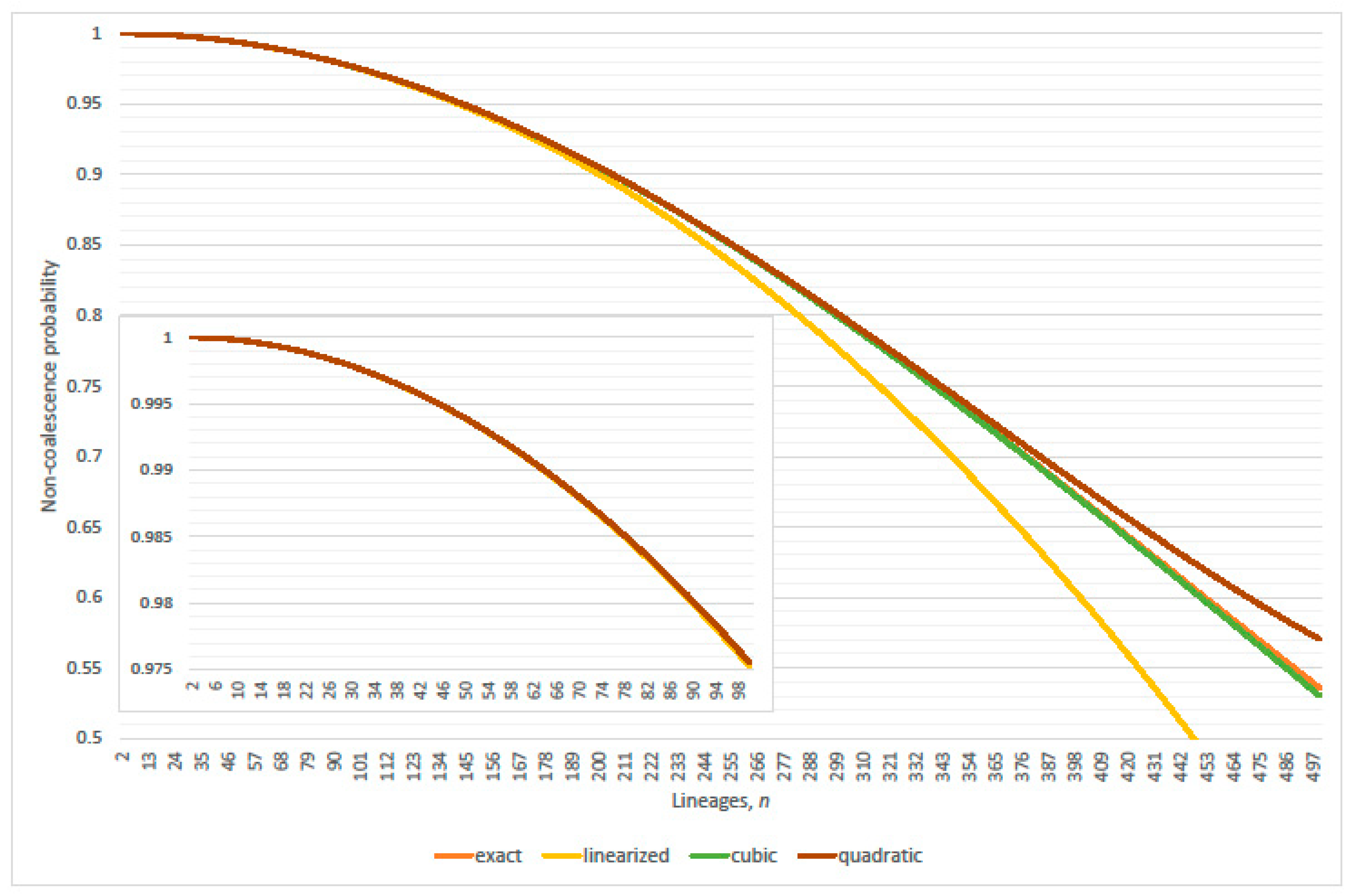
The default population size in this work is set at N = 2 × 10 5 , unless otherwise stated, then the exponent increased and decreased by one or two to verify generality for criterion that are expressed as functions of N. Refer to Figure 1 that compares the first and third order approximation non-coalescence probabilities. The criterion 2 N [16] sets the error tolerance down to where the linearized non-coalescence probability, per generation, goes negative at n = 633 ; clearly, negativity must occur at n ( n 1 ) > 2 N . The criterion N [14] sets the error tolerance greater than 15%, and the corresponding proportion of the exact probability equals 0.825979 at n = 447 . Reduction to precisely 1% error tolerance occurs at n = 233 . Exact non-coalescence probability can be compared to its linearized, quadratic and cubic approximation; refer to Figure 2 and Figure 3. The difference between the quadratic and cubic terms of Equation (4) determines the error of the linearization, since non-linear terms of higher degree do not significantly affect the exact value even with many lineages present in the genealogy; refer to Figure 4. Evaluation of the non-coalescence probability suggests a criterion of 1% proportional error after round-up be N / 3 .
Remark 1.
In this case, coalescence probability absolute error, linearized minus exact value, yields an empirical criterion for greater than (precisely) 99% expected genealogical parity; n 33 . The Wright-Fisher ancestral process restricted to single-pair coalescence thus yields n 34 . The total linearization error of the Kingman coalescent, which includes non-coalescence error, thus yields n 26 . Refer to the exposition of parity in Section 4 for the details of these criteria.

2.2. Single Pair Coalescence Events

Identically to Equation (1), precisely two lineages with the same parent occurs with probability
( n 2 ) N i = 1 n 2 ( 1 i N ) .
The form of Equation (7) can be explained by analogy to Equation (1). Common ancestry among two lineages occurs with probability 1 · 1 N , since the same individual must be picked uniformly at random from the parent generation by two individuals from the offspring generation in a population of fixed size N. Exchangeability renders a combinatorial term ( n 2 ) , since any single pair of the n lineages from the offspring generation participate in such a common ancestry event. There is no common ancestry among the remaining n – 2 lineages in the offspring generation, which yields the corresponding product of ( N i ) / N for i = 1 , 2 , , n 2 .
Compare the linearized probability of at least one coalescence 1 2 n ( n 1 ) N 1 from Equation (2) and the exact pair-wise coalescence probability of Equation (7). Clearly, the linearization omits the corresponding non-coalescence probability product.
Remark 2.
The single-pair coalescence restriction is questionable prima facie with respect to the exact coalescence probabilities, since the complimentary event to non-coalescence in Equation (1) describes at least one coalescence. This includes combinations of single-pairs or multi-coalescence. The N 1 term of Equation (4) linearizes the probability of at least one coalescence, which is to be distinguished from the probability of single pair coalescence.
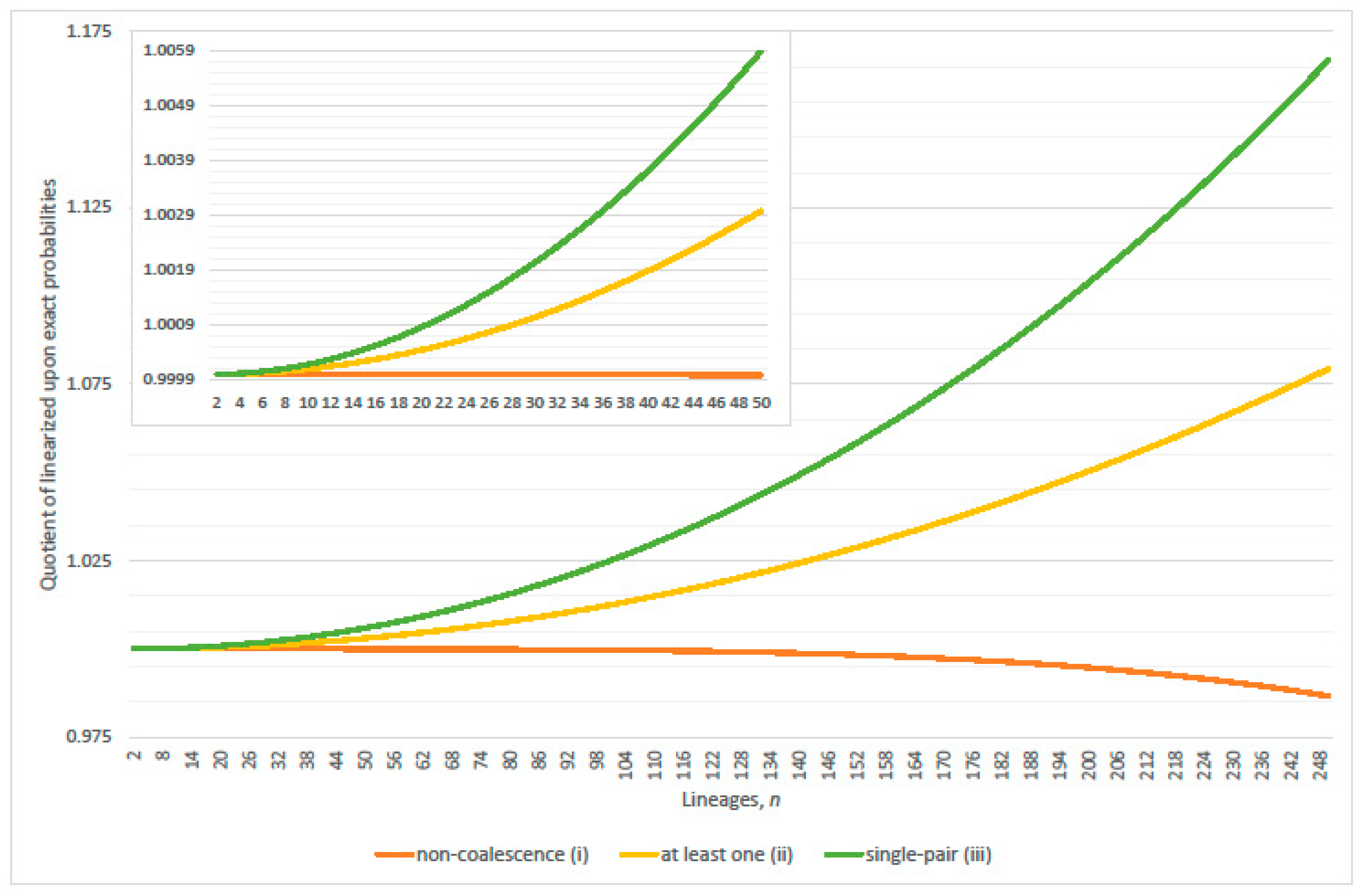
The differences between the corresponding linearized and exact probabilities cancel out as equal and opposite, whereas the relative proportions yield asymmetric linearized substitutions; refer to Figure 5. Both substitutions equal the exact value at n = 2; as n increases, linearized non-coalescence probability underestimates and linearized coalescence probability overestimates. Although the absolute errors have zero sum, linearization exaggerates coalescence transition probabilities and by comparison slightly reduces non-coalescence transition probabilities; refer to Section 2.3. Thus, Kingman’s coalescent detracts from the exact ancestral process.
Table 1 quantifies decreased accuracy of coalescence probability linearization, in Figure 5 (ii), for alternative population sizes, N.
Remark 3.
Does the conventional substitution correspond to omission of the multi-coalescence probabilities, or constraint of emergent coalescence events by suppression of multi-coalescence and replacement with single pair coalescence? Answer: The latter, since the probability of at least one coalescence is linearized in Equation (1).
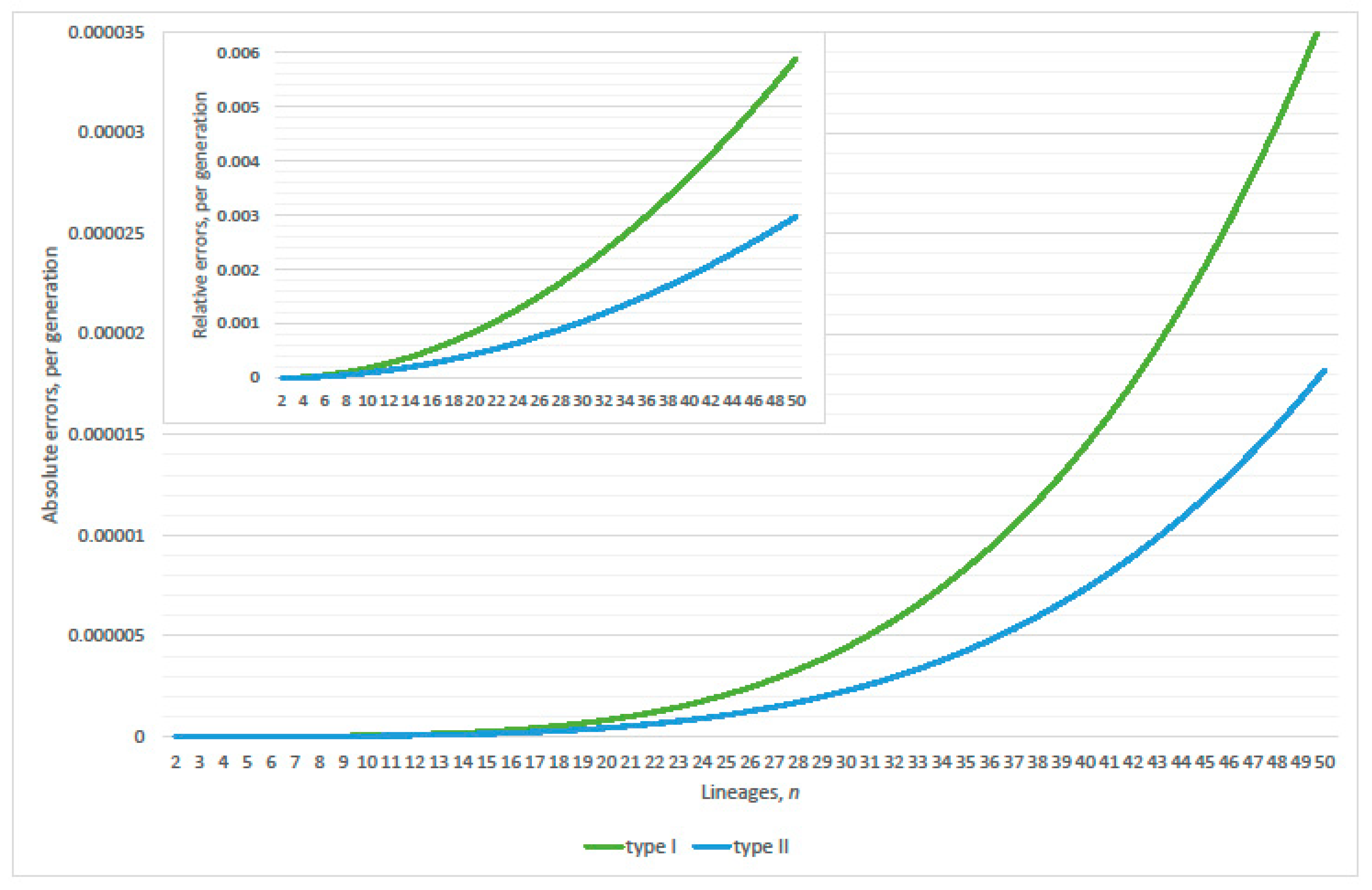
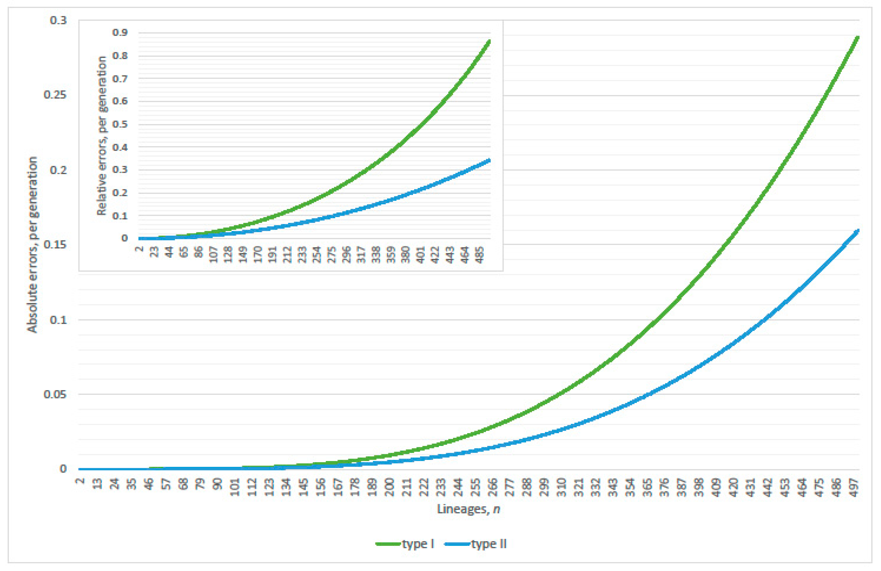
Define the absolute error (type I) as the difference between linearized and exact single pair coalescence probabilities; ( n 2 ) / N minus Equation (7). The quotient of the absolute error (type I) upon the exact single pair coalescence probability defines the relative error (type I). After cancellation, when n lineages remain, this equals the quotient of exact probabilities for at least one coalescence upon non-coalescence from n 2 lineages. Alternatively, define absolute error (type II) as the difference between linearized and exact at least one coalescence probabilities; ( n 2 ) / N minus the probability of the complimentary event to Equation (1). The quotient of the absolute error (type II) upon the exact at least one coalescence probability defines the relative error (type II). Refer to Equations (14) and (16) in Section 4 for further explanation.
The absolute and relative errors heighten a probability structure that would be invisible otherwise; refer to Figure 6 and Figure 7. Thus, the robustness of the Kingman coalescent gets a qualitative measure. The quotient of relative errors illustrates their comparative proportional growth as n increases; refer to Figure 8. In this case, a minmax transition occurs around n = 20 between two gradient phases that correspond to the quotients of relative error type I upon type II. Intuitively, the two types of relative errors follow maximum and minimum detraction, respectively; type I corresponds to suppression of multi-coalescence altogether, whereas type II corresponds to replacement of multi-coalescence events with a single-pair, which accords to the Kingman coalescent. The single-pair and at least one coalescence probabilities for small to moderate numbers of lineages look equivalent; refer to Figure 9 in Section 2.3.
Relative error (type II), per generation, does not exceed precisely 1% where n 90 , in this case.

2.3. Multiple Coalescence Events

There is no implementation of multiple coalescence events in fastsimcoal, version 2.6 (fsc26), according to their online documentation [39,40,41]. Extension of an original SimCoal package [42] simulates genetic data serially sampled, Serial SimCoal [43], and implements a heuristic double-pair coalescence transition probability (software and documentation available online: http://web.stanford.edu/group/hadleylab/ssc/index.html).
Consider the ancestral process in which at coalescence a decrement of two lineages can occur; double-pair or triplet coalescence. Precisely two pairs of lineages, with a different parent in common for each pair, occurs with probability
1 2 ( n 2 ) ( n 2 2 ) N 2 i = 1 n 3 ( 1 i N ) ,
since discounting permutation of both pairs yields a factor one half. Similar with Equation (7), precisely one pair-wise common ancestry event occurs with probability ( n 2 ) / N , since this event involves any two of the n lineages present in the offspring generation. The second pair-wise common ancestry event picks a different common parent to the first pair and this occurs with probability ( N 1 N ) 1 N ( n 2 2 ) . Permutation of the first and second pairs does not count due to the exchangeability of lineages in the ancestral process and requires the factor ½. There is no common ancestry among the remaining n − 4 lineages in the offspring generation, which yields the corresponding product of ( N i ) / N for i = 2 , 3 , , n 3 .
Three lineages with the same parent occurs with probability
( n 3 ) N 2 i = 1 n 3 ( 1 i N ) .
Common ancestry among three lineages occurs with probability 1 · 1 N · 1 N , since the same individual from the parent generation is picked uniformly at random by three individuals from the offspring generation in a population of fixed size N. Exchangeability renders a combinatorial term ( n 3 ) , since any triplet of the n lineages from the offspring generation participate in such a common ancestry event. There is no common ancestry among the remaining n 3 lineages in the offspring generation, which yields the corresponding product of ( N i ) / N for i = 1 , 2 , , n 3 .
Consider the ancestral process in which at coalescence a decrement of three lineages can occur; triple-pair, both a single-pair and a triplet, or quadruplet coalescence. Three pairs of lineages, with a different parent in common for each pair, occurs with probability
1 3 ! ( n 2 ) ( n 2 2 ) ( n 4 2 ) N 3 i = 1 n 4 ( 1 i N ) ,
since discounting permutation of the triple-pair yields a factor one sixth. Similar with Equation (8), the first pair-wise common ancestry event occurs with probability ( n 2 ) / N . The second pair-wise common ancestry event picks a different common parent to the first pair and this occurs with probability ( N 1 N ) ( n 2 2 ) / N . The third pair-wise common ancestry event picks a different common parent to the first and second pairs and this occurs with probability ( N 2 N ) ( n 4 2 ) / N . Permutation of the first, second and third pairs does not count due to the exchangeability of lineages in the ancestral process and requires the factor ⅙. There is no common ancestry among the remaining n 6 lineages in the offspring generation, which yields the corresponding product of ( N i ) / N for i = 3 , 4 , , n 4 .
One single-pair and one triplet of lineages, with a different parent in common, occurs with probability
1 2 ( n 2 ) ( n 2 3 ) N 3 i = 1 n 4 ( 1 i N ) ,
since discounting permutation of the pair and the triplet yields a factor one half. The pair-wise common ancestry event occurs with probability ( n 2 ) / N . Similar with Equation (9), the triplet common ancestry event now picks a different common parent to the pair and this occurs with probability ( N 1 N ) 1 N 1 N ( n 2 3 ) . The alternative combinatorial product ( n 3 ) ( n 2 2 ) yields the same function of n as in Equation (11). In this sense, the two alternatives cannot be distinguished. However, the usual permutation discount of simultaneous common ancestry events, one single pair and one triplet, applies with the factor ½ due to exchangeability. There is no common ancestry among the remaining n − 5 lineages in the offspring generation, which yields the corresponding product of ( N i ) / N for i = 2 , 3 , , n 4 .
Precisely four lineages with the same parent occurs with probability
( n 4 ) N 3 i = 1 n 4 ( 1 i N ) .
Common ancestry among four lineages occurs with probability 1 · 1 N · 1 N · 1 N , since the same individual from the parent generation is picked uniformly at random by four individuals from the offspring generation in a population of fixed size N. Exchangeability renders a combinatorial term ( n 4 ) , since any quadruplet of the n lineages from the offspring generation participate in such a common ancestry event. There is no common ancestry among the remaining n − 4 lineages in the offspring generation, which yields the corresponding product of ( N i ) / N for i = 1 , 2 , , n 4 .
The probabilities of Equations (7)–(12) constitute a subset of all possible types of coalescences and therefore yield a restricted ancestral process. These probabilities correspond in every generation until a coalescence event occurs, with those of certain multi-coalescences equal to zero for small n. That is, such probabilities apply from one generation to the next among the offspring while n lineages remain. At coalescence, adjust n accordingly and continue the ancestral process, until eventually absorption occurs with a most recent common ancestor of the entire initial sample.
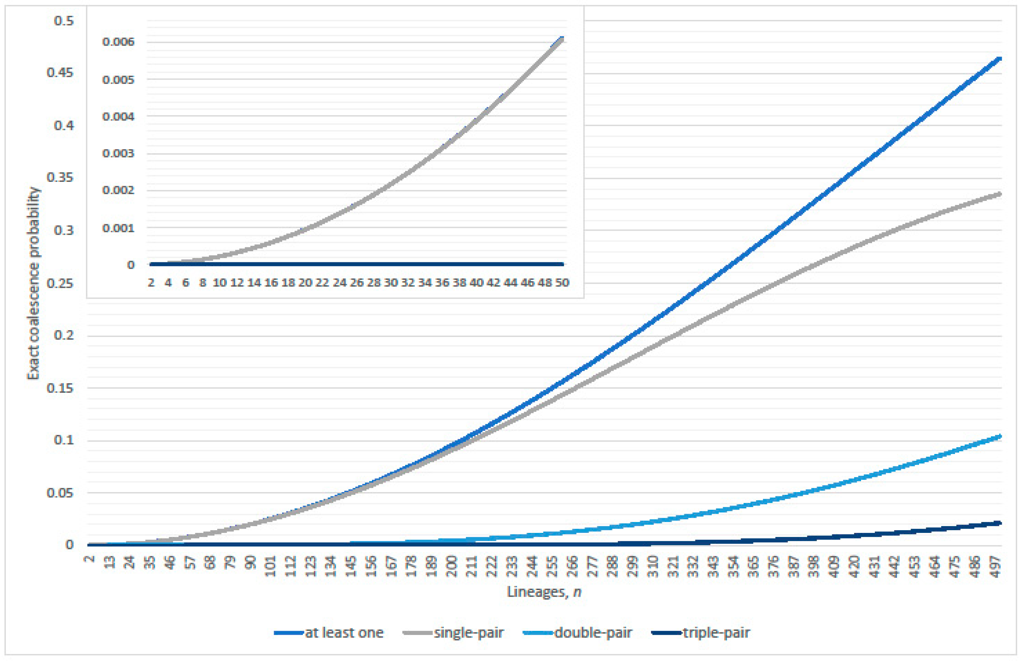
The exact at least one coalescence probability, compliment to Equation (1), and multiple exact coalescence probabilities of Equations (8) and (10) evaluated for small, moderate and larger numbers of lineages demonstrate their region of negligibility; refer to Figure 9.
The significance of coalescence probabilities of Equations (7)–(12) is of direct relevance to computer simulation and importance sampling methodology of the ancestral Markov chain, particularly as linearization errors accumulate. For the present purpose, quantitative analysis of conditional coalescence probability given the event of at least one coalescence, compliment to Equation (1), occupies Section 3.1.

3. Genealogical Topology and Expected Inter-Arrival Generations

Realization of the entire ancestral process yields one resultant genealogy. Statistical inference of genealogical time, for instance importance sampling methodologies, should be robust under a subset of ancestral transitions restricted to lineage decrements of one unless other genetic or exogenic processes act to emphasize the external branches.

3.1. Conditional Probabilities of Multi-Coalescence

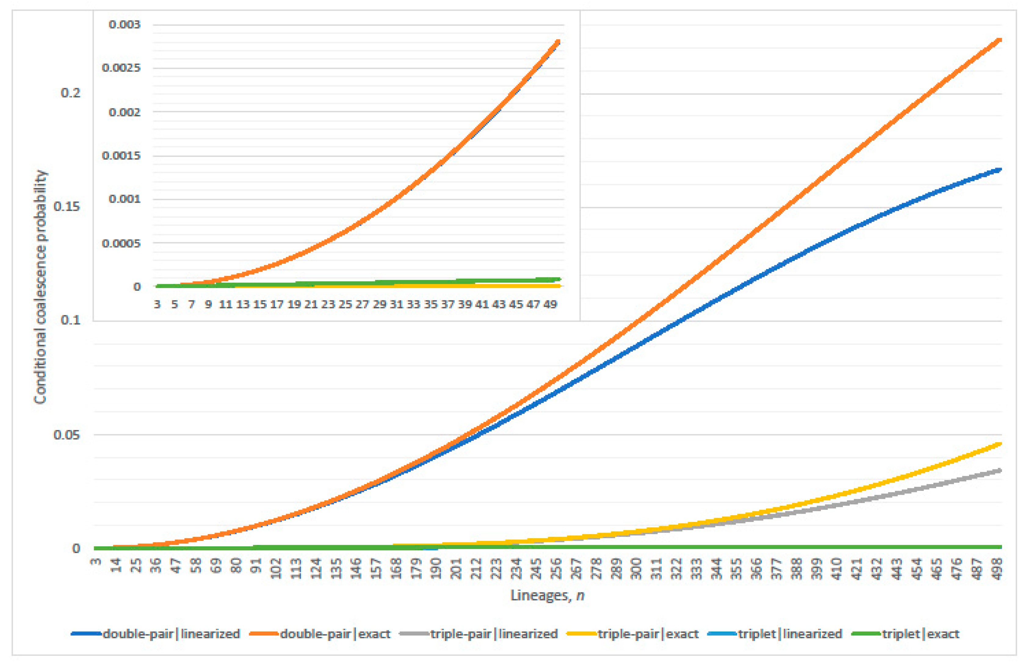
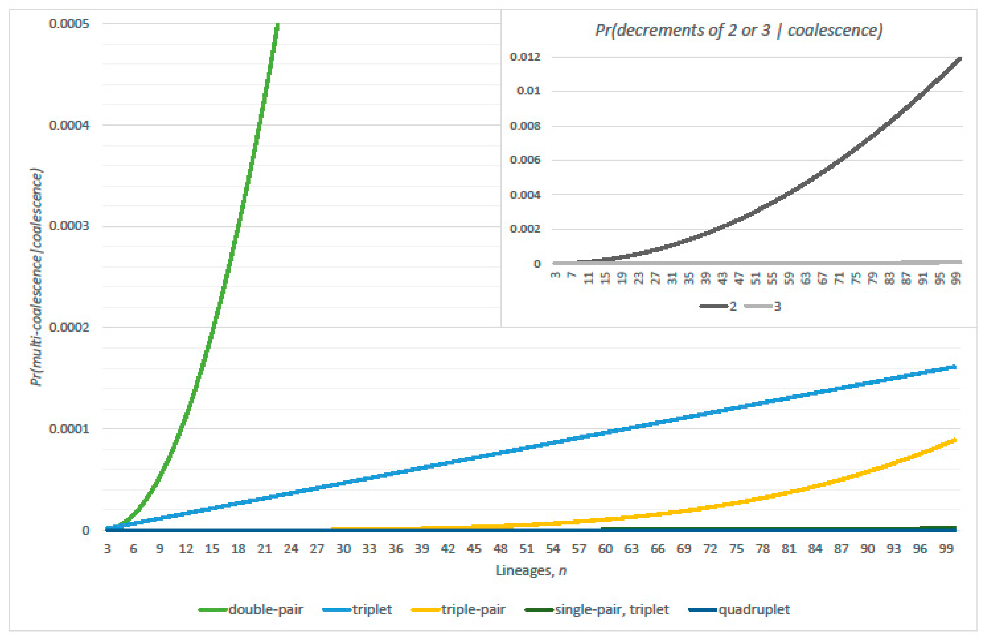
The conditional probability of multi-coalescences given a coalescence event determine the genealogical topology in realization of the ancestral process. Refer to Figure 10, where conditional probability is given the event of at least one coalescence, either linearized or exact. Given exact coalescence: when n = 10, Pr(double-pair | coalescence) < 1/14,286, Pr(triplet | coalescence) < 1/75,003 and Pr(triple-pair | coalescence) < 1/571,428,571. When n = 20, 1/2615, 1/33,344 and 1/13,071,895, respectively. Thus, in the region of most significance to timing, such multi-coalescence events rarely occur under genealogical stochastic reiteration.
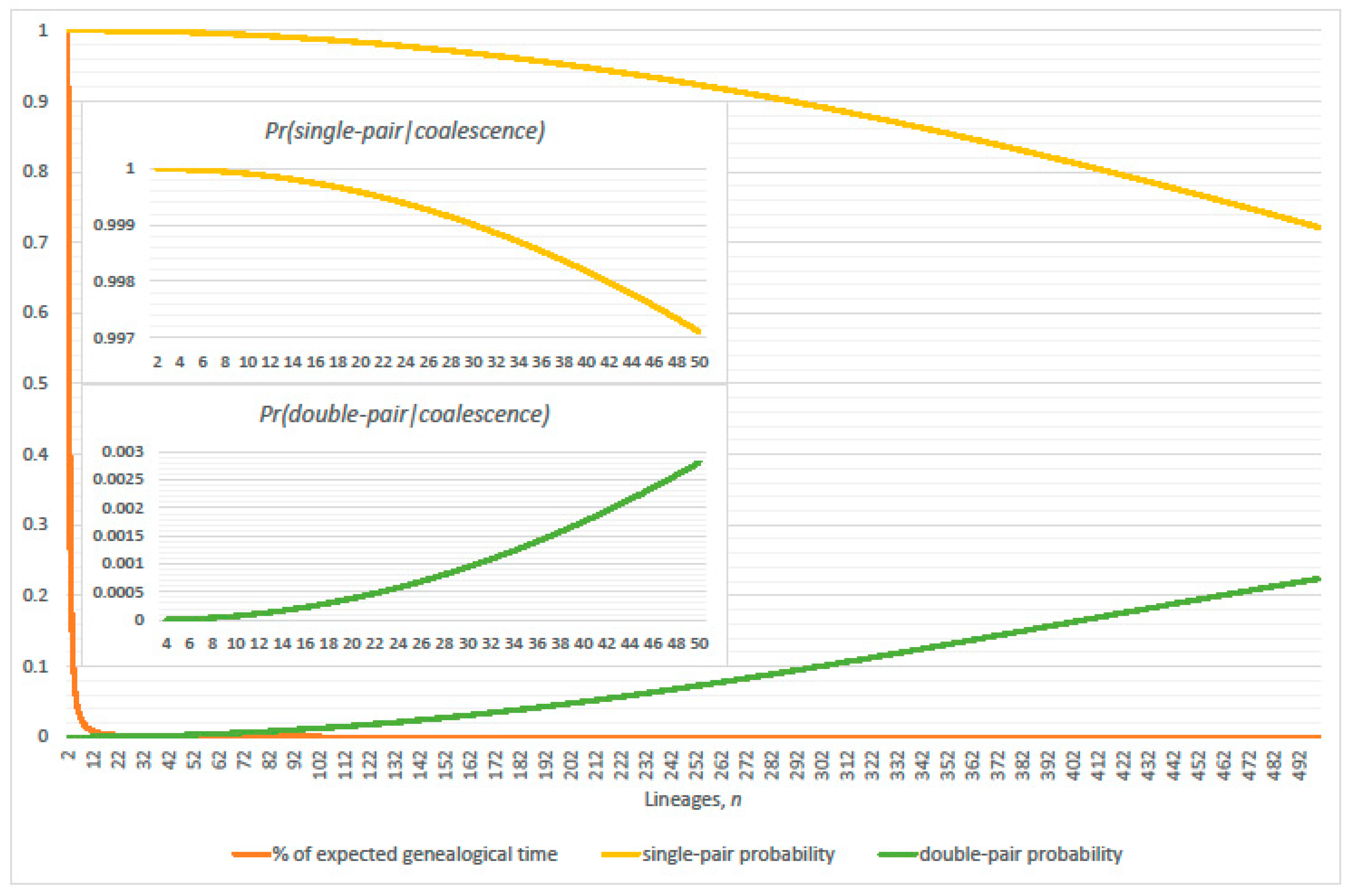
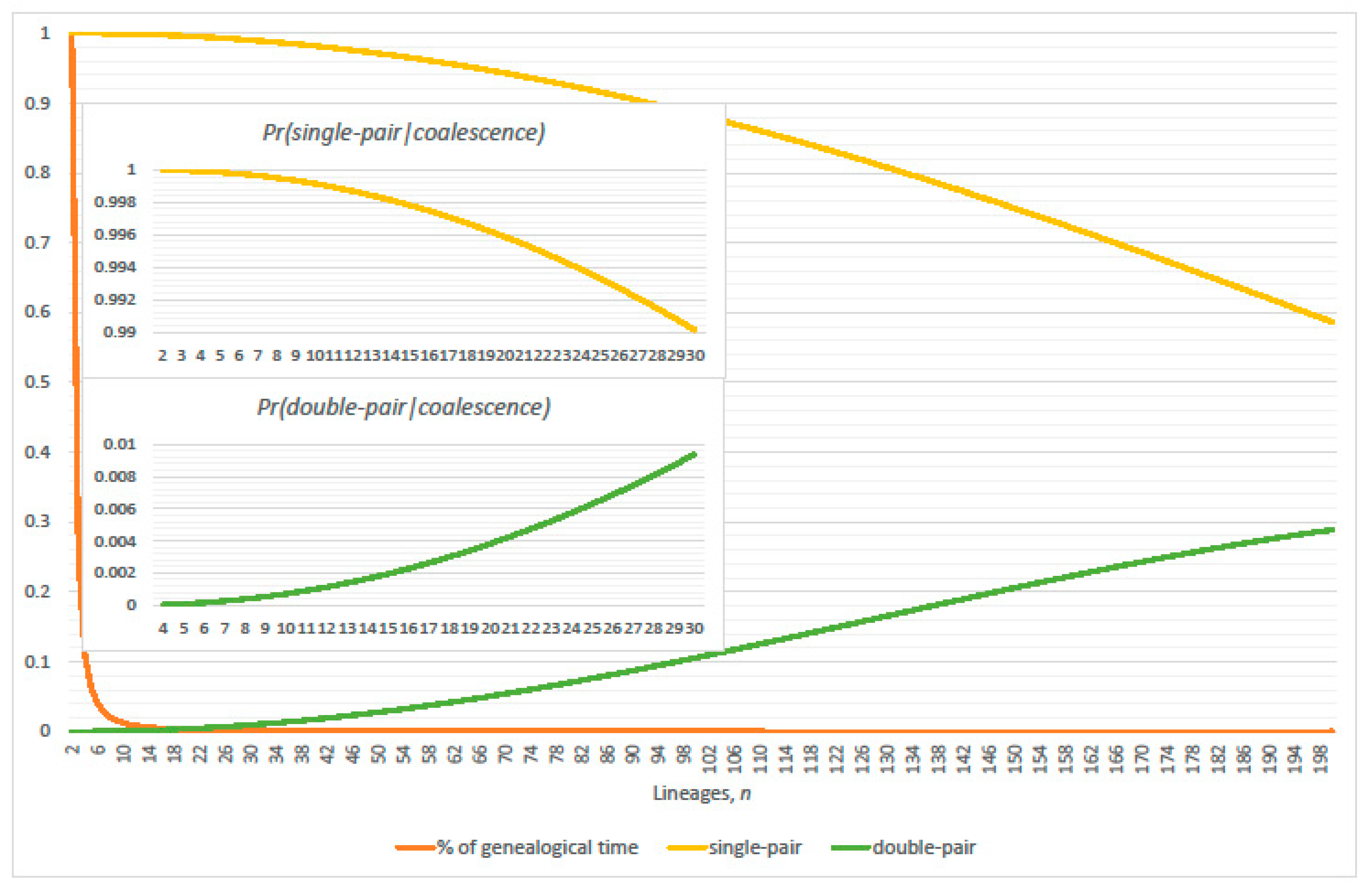
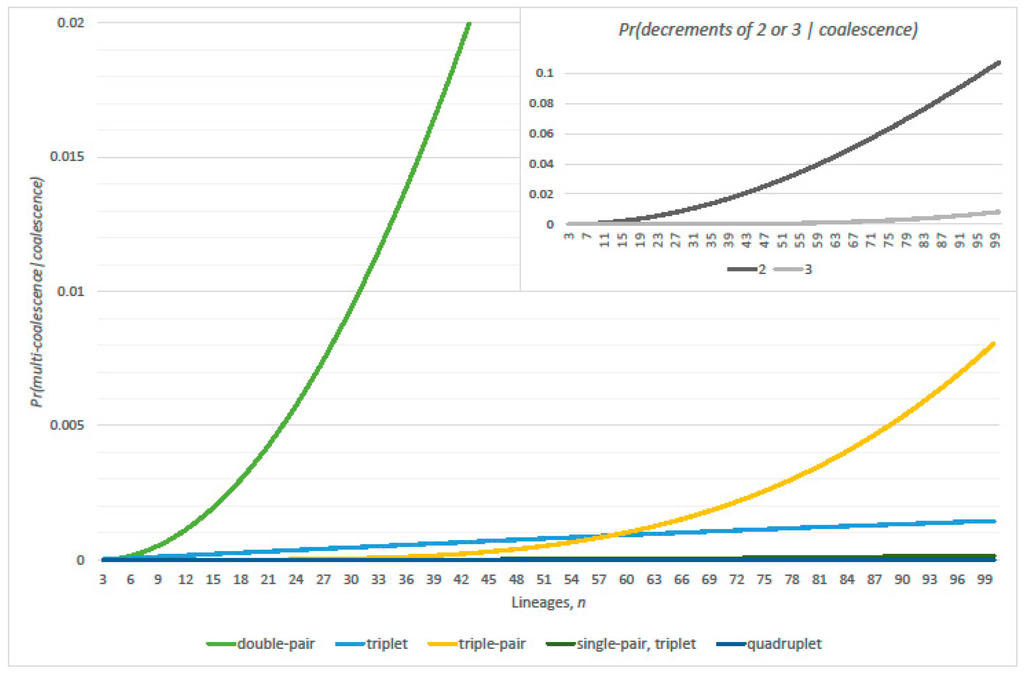
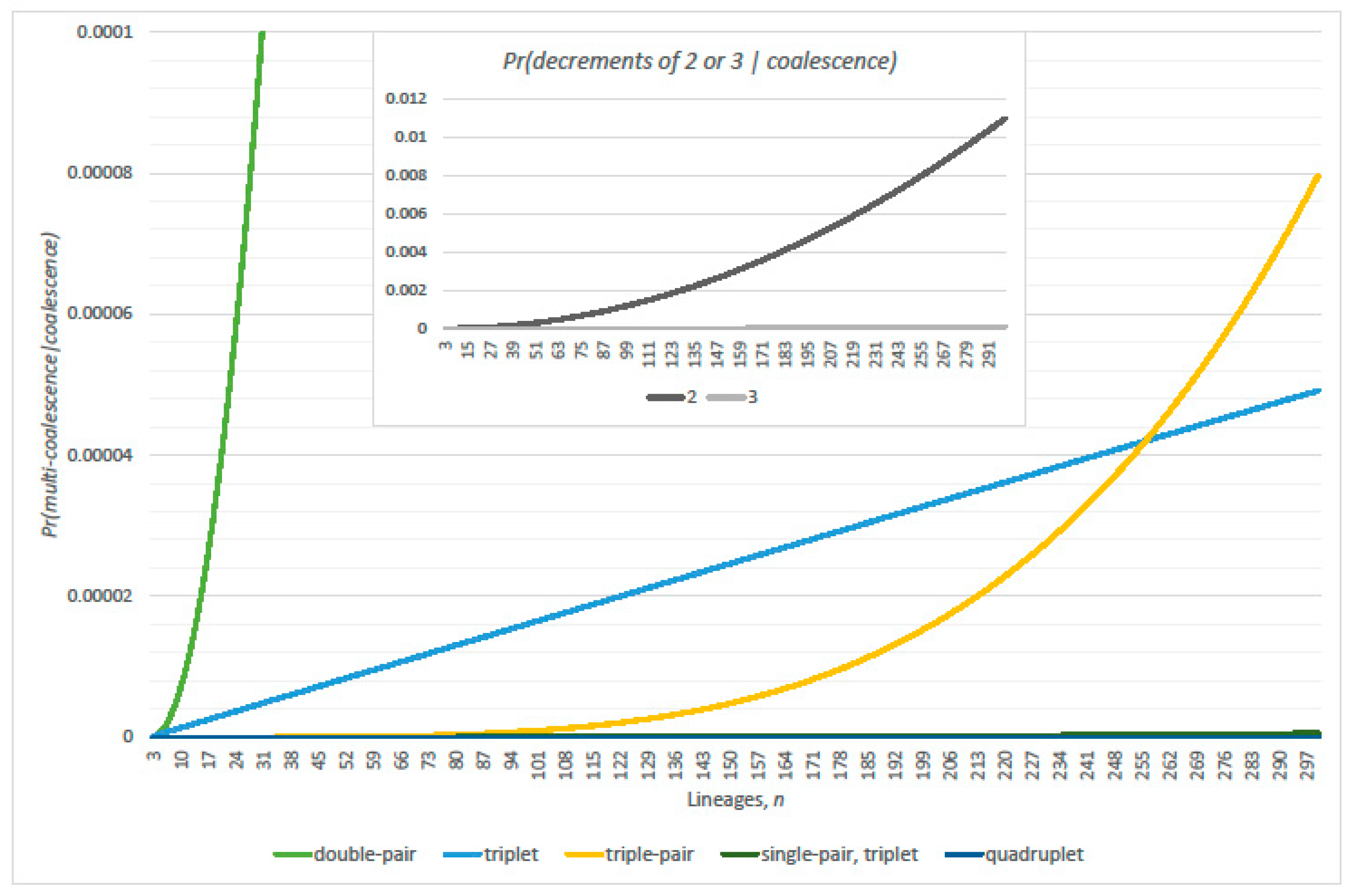
Figure 11, Figure 12 and Figure 13 illustrate the rapid decline of significant intervals for timing the genealogy and quantify the extent of multi-coalescence event rarity. Multi-coalescence event probabilities vary substantially within such regions, and negligibility becomes less extensive as population size decreases; refer to Figure 14, Figure 15 and Figure 16.
In the first regions, these conditional probabilities of triplets exceed triple-pairs; this trend switches in the second regions and triple-pairs far exceed triplets. Thus, only the slightest relative contribution of multiple coalescence transition probabilities occurs in the ancestral process, per generation. Substantial replication of the ancestral process will be required before realizing a genealogy that contains multi-coalescence events. That is, unless the genealogy consists of many lineages or the population size is diminished substantially.

3.2. Single-Pairs Dominate Double-Pairs?

Consider the relative probabilities of double-pair and single-pair coalescence, namely the quotient of Equation (8) upon Equation (7),
( n 2 ) ( n 3 ) 4 N 4 ( n 2 ) .
Equation (13) equals case i = 1 [16] (Equation (19)), which required correction since it should be ( n 2 i ) ( n 2 i 1 ) / [ 2 N ( i + 1 ) 2 ( i + 1 ) ( n i 1 ) ] , where the denominator term 2N(i + 1) replaces 4N(i + 1). This expression equals the quotient of the (i + 1)st multiple and the ith multiple-pair coalescence probability. Thus, i = 1 corresponds to the quotient of double-pair upon single-pair coalescence probabilities.
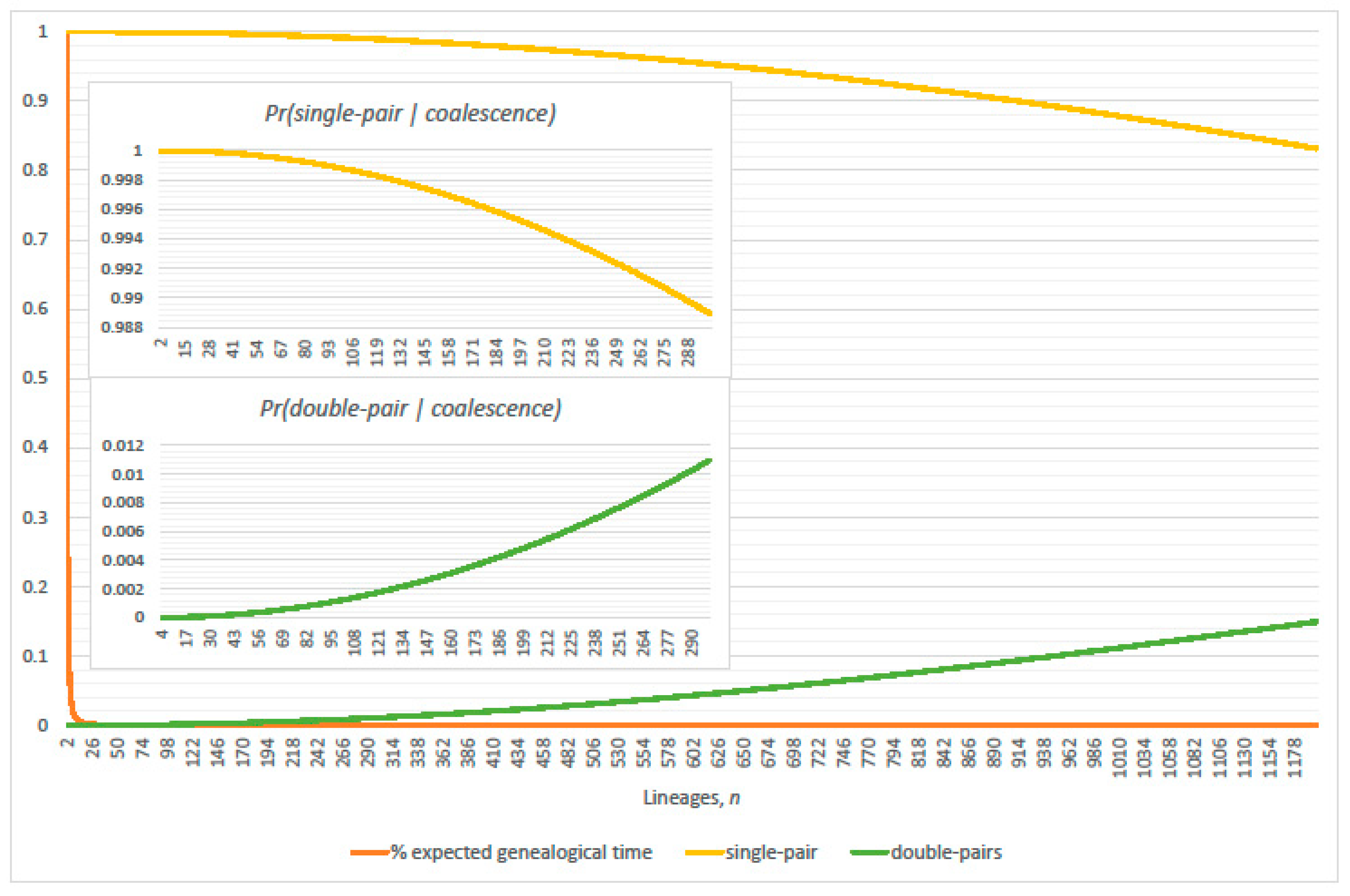
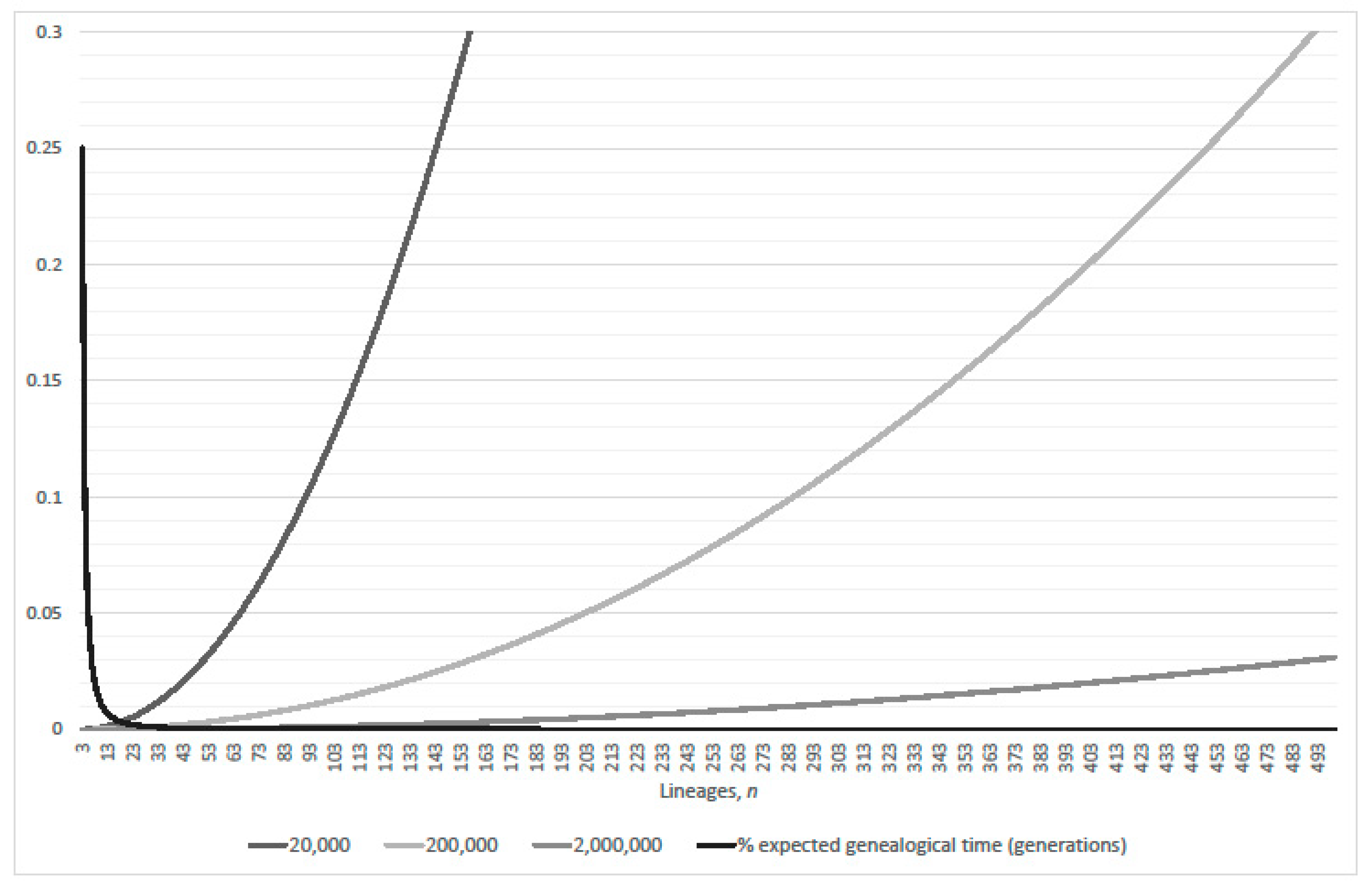
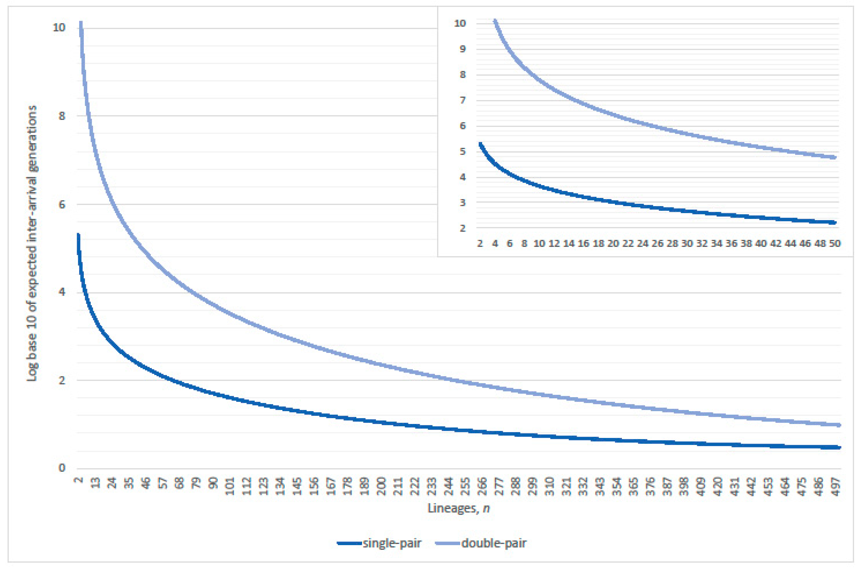
The quotient of Equation (13) explains the dominance of expected inter-arrival times by single-pair coalescence. This is because the geometric distribution yields expectation equal to the reciprocal of the sum of Equation (7) plus Equation (8), when double and single-pair coalescences may occur in the ancestral process. Thus, double-pair coalescence is negligible in terms of the expected inter-arrival generations in the ancestral process due to Equation (13). Refer to Figure 17, the quotient of double-pair upon single-pair coalescence probabilities per generation has increased from nil at n = 2 to 1% (0.1%, N = 2,000,000) at n = 92, whereas the relative proportion of the total expected generations in the genealogy then equals 0.0121%. The expected inter-arrival generations determined by single-pair and double-pair coalescence probability, respectively, equals 1 / p s of Equation (7) and 1 / p d of Equation (8); refer to Figure 18. The exact probability of avoiding a double-pair coalescence per expected interval, according to the geometric distribution with parameter p d at n = 92 equals 0.990032.
In the next Section, calculation of multiple coalescence event probabilities per expected interval leads to a paradox of negligibility and its resolution obtained.

4. Parity of the Kingman Coalescent

Empirical calculations in this section yield a criterion of coalescence probability error, linearized minus exact value, such that expected genealogical parity be greater than 99% where n 1 2 N 3 . The Wright-Fisher ancestral process restricted to single pair coalescence empirically yields the same criterion as that just described. Total error of the Kingman coalescent that includes linearized non-coalescence probability thus yields 1 2 N / 2 3 .
In general, per generation, consider error to be the probability of a neglected coalescence; parity the probability of avoiding a neglected coalescence. The parity, per expected interval, is obtained by raising parity, per generation, to the power of an exponent given by 1/p, where p equals the probability of coalescence, per generation. For instance, using the linearized coalescence probability yields the expected inter-arrival generations of Kingman’s coalescent. The product of parity, per expected interval, across all intervals from the initial sample to its most recent common ancestor yields expected genealogical parity. Non-occurrence of neglected coalescence events anywhere in the expected genealogical realization represents perfect parity. This maximum stringency confounds observability, since the impact of neglected coalescence depends on position within the genealogy. Therefore, parity, per expected interval, is more directly informative.

4.1. Linearization Errors

The linearization of Kingman’s coalescent yields error in both the non-coalescence and the coalescence probabilities, which cancel each other and sum to zero when the coalescence error is with respect to the exact probability of at least one coalescence. Consider n lineages to be present in the genealogy. Define the linearization error (type I) with respect to the exact probability of single-pair coalescence, per generation,
{ { 1 ( n 2 ) N } i = 1 n 1 ( 1 i N ) } + { ( n 2 ) N ( n 2 ) N i = 1 n 2 ( 1 i N ) } .
Equation (14) simplifies as the exact multi-coalescence probability and is equivalent to the error of the Wright-Fisher ancestral process restricted to single-pair coalescence. Thus, one minus the linearization error (type I) defines linearization parity (type I), per generation,
[ 1 + ( n 1 ) ( n 2 ) 2 N ] i = 1 n 2 ( 1 i N ) .
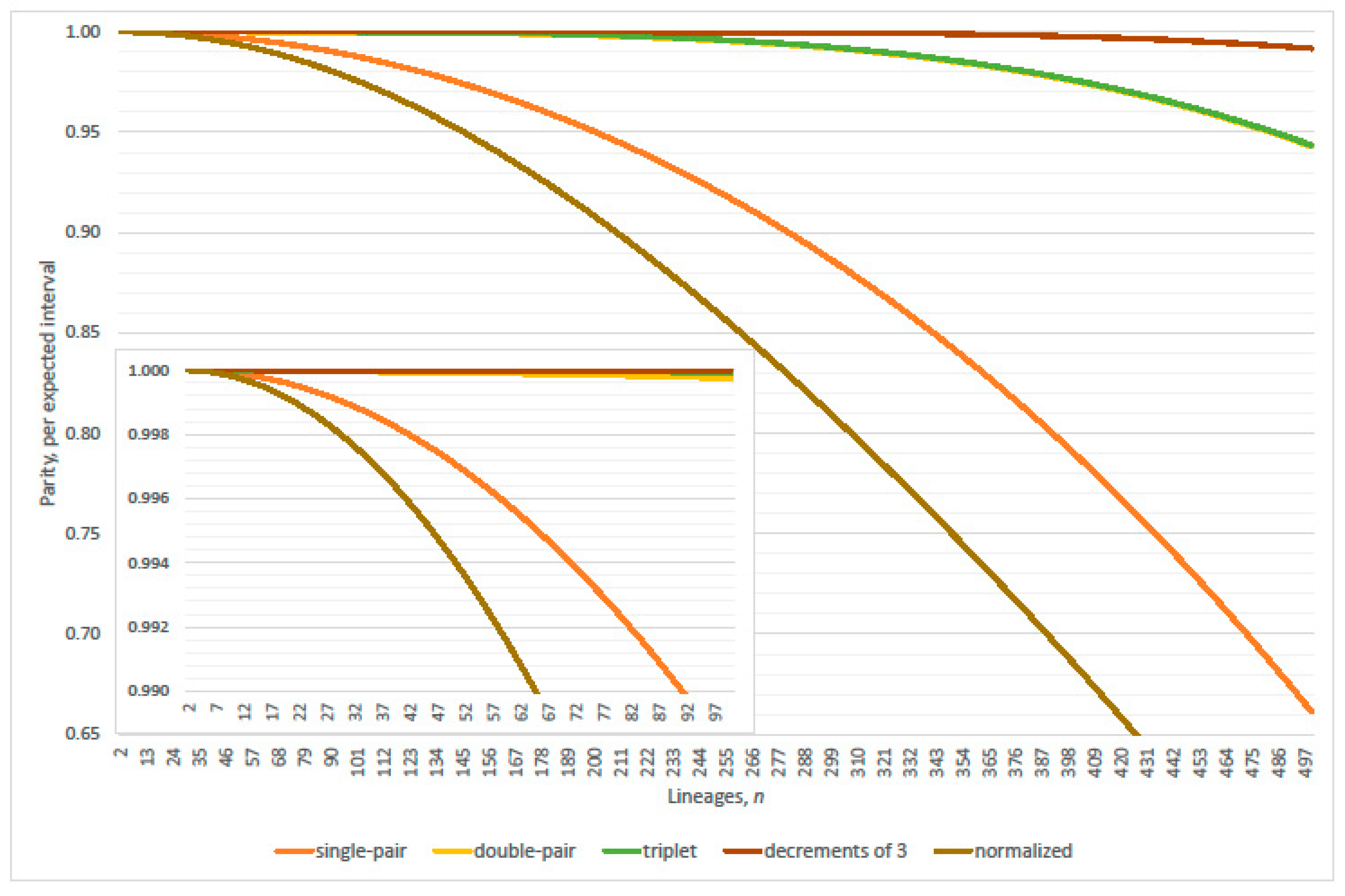
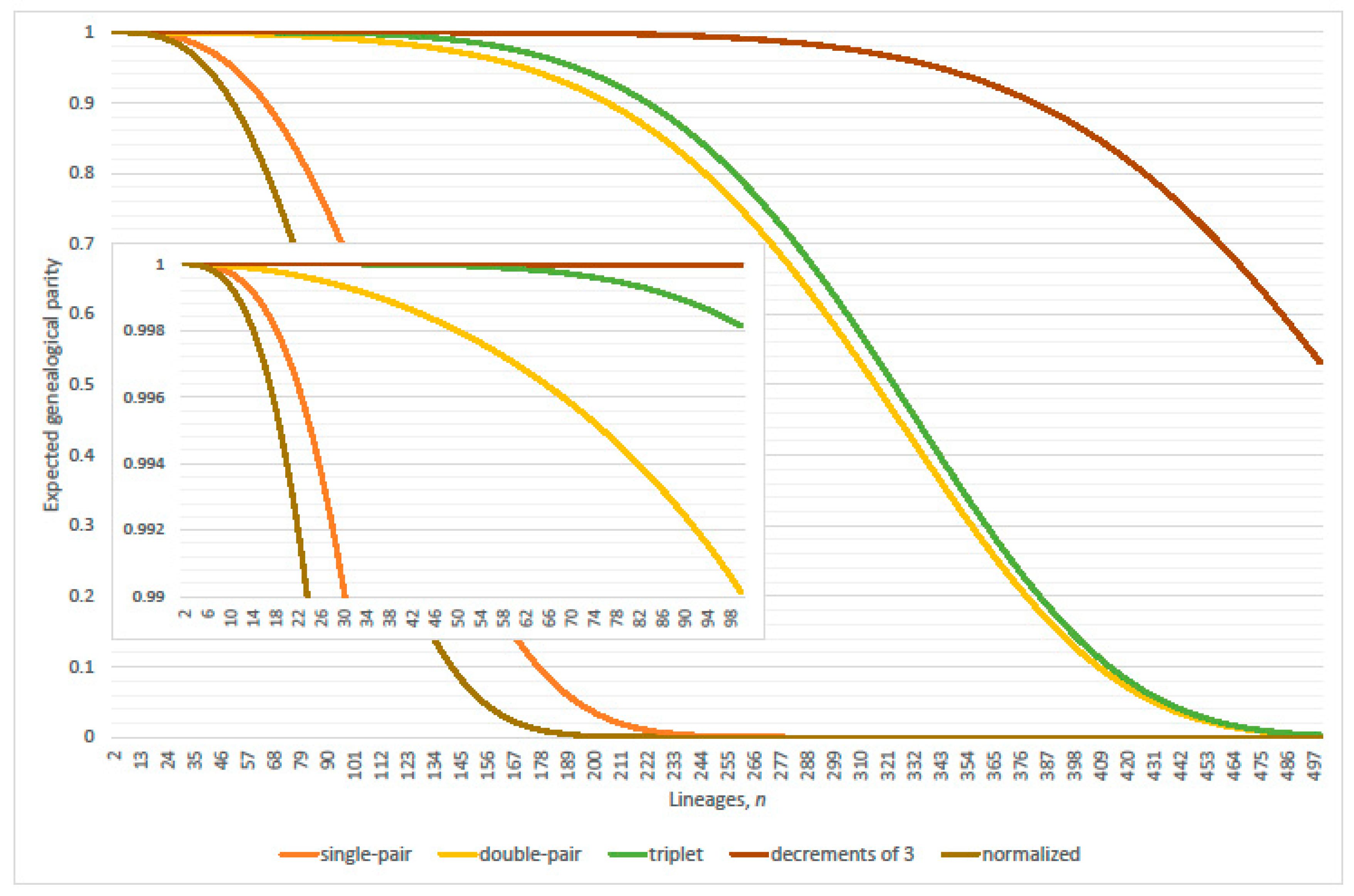
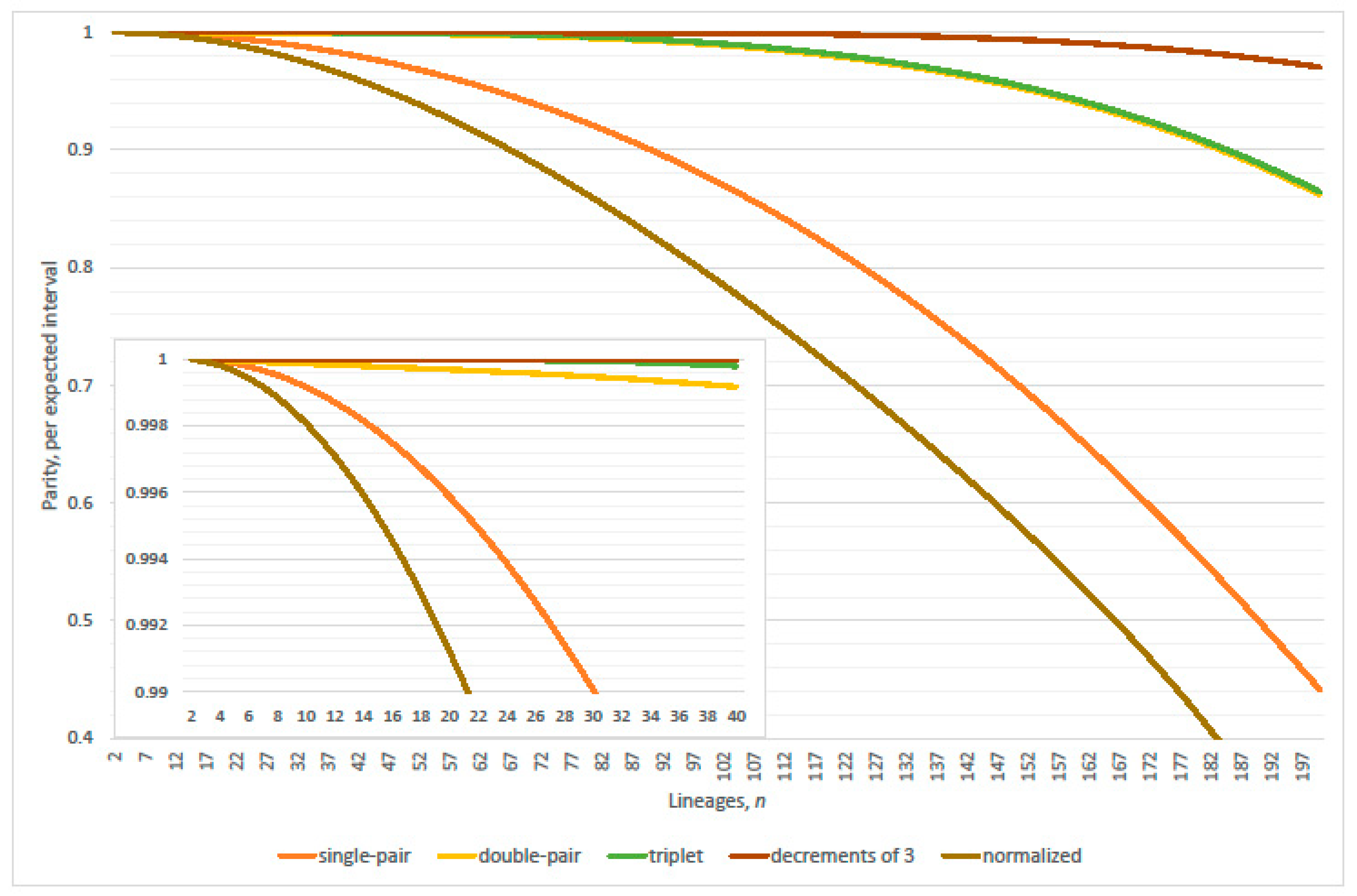
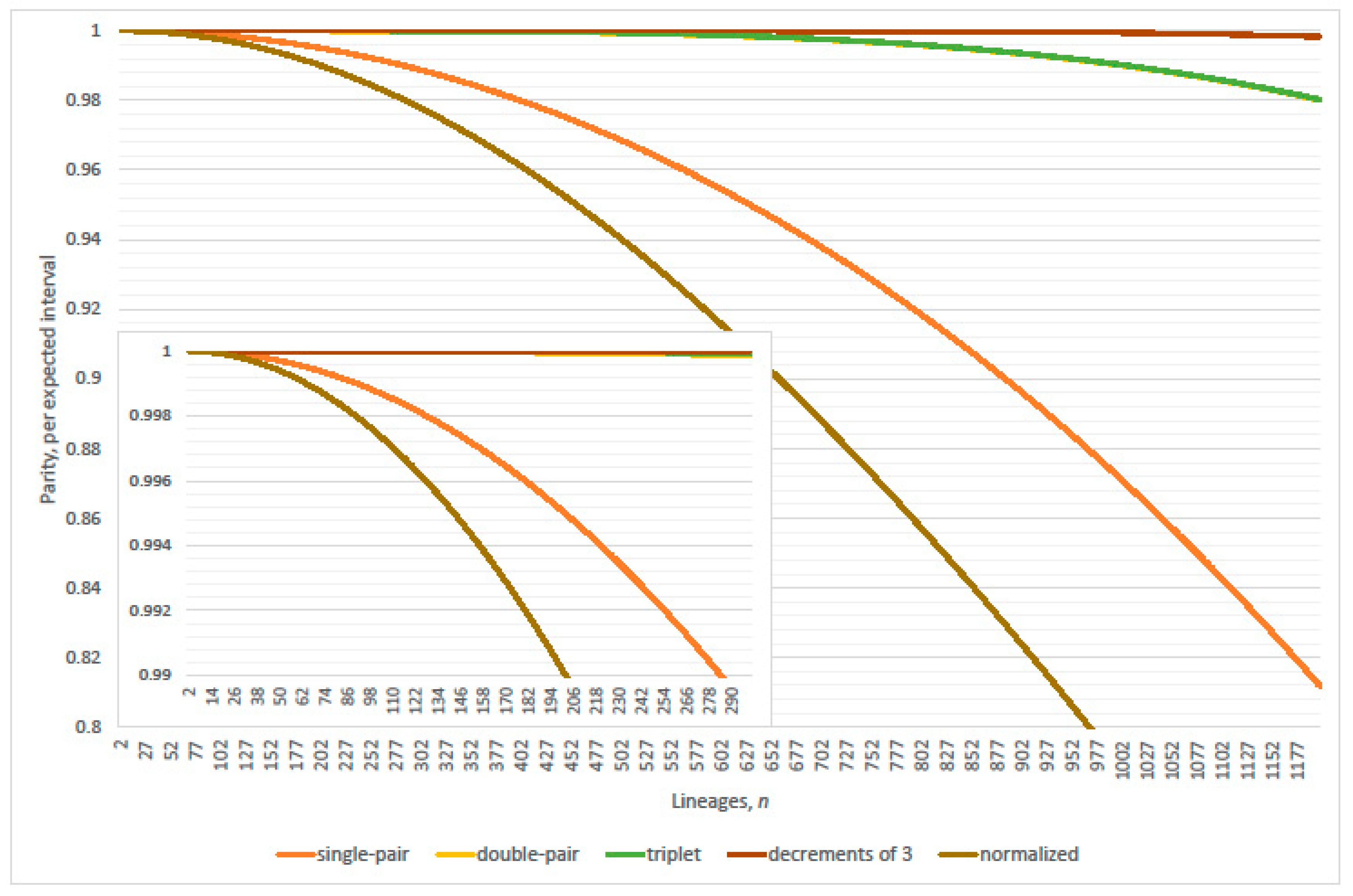
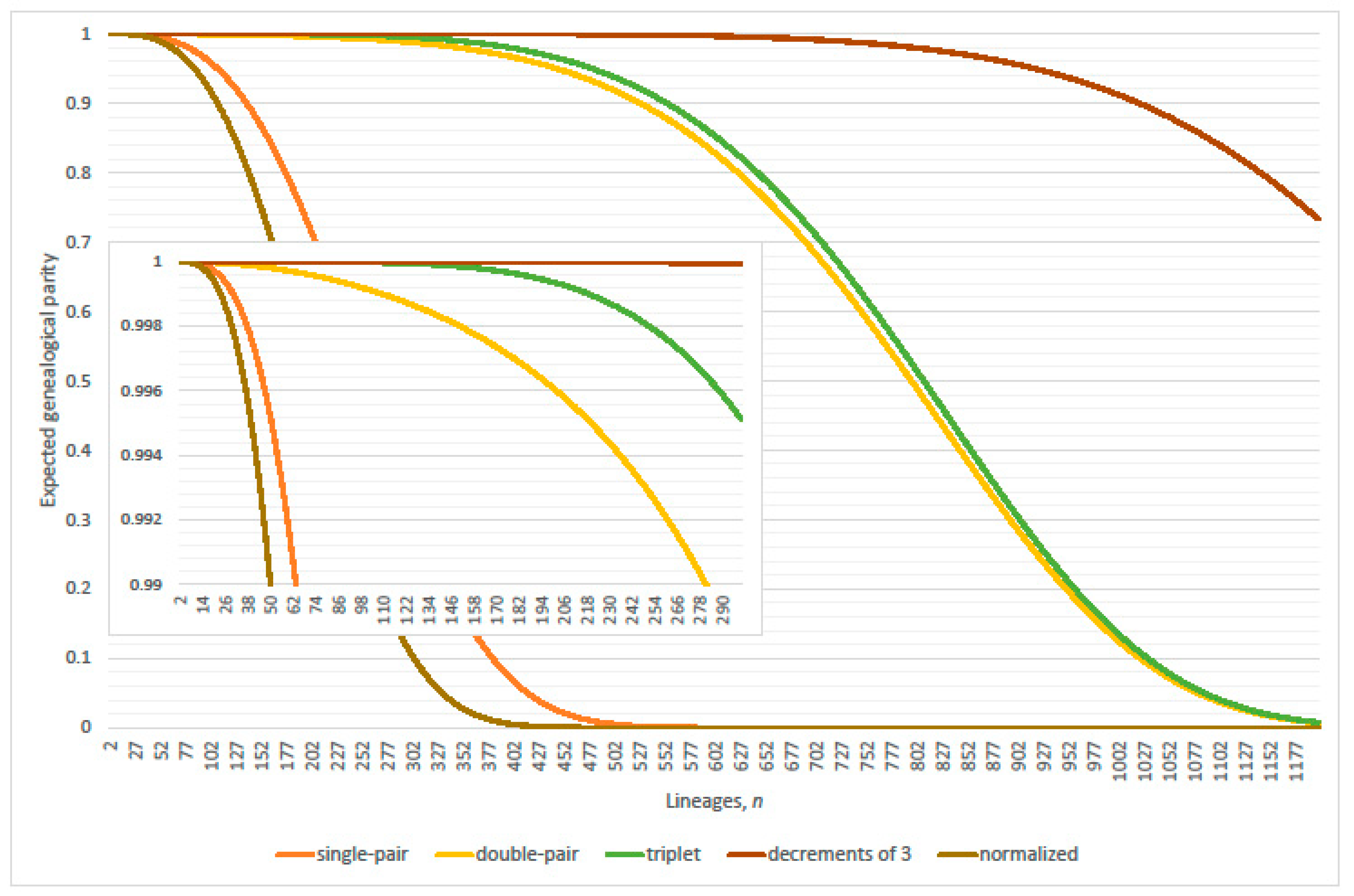
Note Equation (15) equals one plus the linearized coalescence probability then multiplied by the exact non-coalescence probability, while n − 1 lineages remain in the genealogy. Equation (15) is quantified as n varies, per expected interval and expected cumulative genealogy, according to reduced, mid-range and enlarged constant population sizes in Figure 19, Figure 20, Figure 21, Figure 22, Figure 23 and Figure 24. These Figures also illustrate that inclusion of multi-coalescence transition probabilities of Equations (8)–(12) sustain parity of restricted Wright-Fisher models.
Ancestral process of restricted Wright-Fisher models:
In the single-pair exact ancestral process, parity, per expected interval, exceeds precisely 99% where n 91 ; refer to Table 2. An identical criterion was observed with relative error (type II) of the linearized coalescence probability; refer to Section 2.1. In the single- or double-pair exact ancestral process, parity, per expected interval, exceeds precisely 99% where n 316 .
Values in Table 2 signal a clear loss of parity in the single-pair restricted Wright-Fisher model.
Empirical criteria of the single-pair restricted Wright-Fisher model, linearization parity (type I):
  • parity, per expected interval, exceeds 99% where (approximately) n 1 2 N / 6
    (Table 2 verified this case where N = 2000; 20,000; 200,000; 2,000,000 and 20,000,000); and
  • expected genealogical parity exceeds 99% where n 1 2 N 3
    (precise, N = 20,000 and 200,000; plus one, N = 2,000,000 and 20,000,000; minus one, N = 2000).
Otherwise, define the linearization error (type II), per generation,
{ { 1 ( n 2 ) N } i = 1 n 1 ( 1 i N ) } + { ( n 2 ) N [ 1 i = 1 n 1 ( 1 i N ) ] } 0 .
The constituent errors in Equation (16) have opposite polarity. Heuristically, reverse the sign of the underestimated non-coalescence probability then add the overestimated coalescence probability to obtain a normalized error (type II). Thus, one minus the normalized error (type II) defines normalized parity (type II), per generation,
3 n ( n 1 ) N 2 i = 1 n 1 ( 1 i N ) .
Equation (17) is quantified as n varies, per expected interval and expected cumulative genealogy, according to reduced, mid-range and enlarged constant population sizes in Figure 19, Figure 20, Figure 21, Figure 22, Figure 23 and Figure 24.
Empirical heuristic criteria of Kingman’s coalescent:
  • parity, per expected interval, exceeds 99% where n 1 4 N / 3
    (normalized parity criterion, per expected interval: n minus one N = 2000, 20,000; plus one 200,000; plus two 2,000,000; overestimates maximum lineages by 1.49% when 20,000,000); and
  • expected genealogical parity exceeds 99% where n 1 2 N / 2 3
    (normalized expected genealogical parity criterion: precise, N = 2000, 20,000, 200,000 and 2,000,000; n plus one when 20,000,000).
Parity criteria of linearization coalescence error (type II) essentially equals that observed with linearization error (type I); verified with N = 20,000, 200,000, and 2,000,000. Parity based on linearization coalescence error (type II) is realistic since application of the Kingman coalescent usually involves only linearized coalescence probabilities with non-coalescence probabilities implicitly assumed.
Remark 4.
Pr(decrement of 2 | coalescence) rises to 1% at n lineages when parity, per expected interval, falls to 99%; verified as N varies. An alternative interpretation of this coupling is that the fractional cubic root criterion of expected genealogical parity occurs at values of n lineages where multi-coalescence transitions remain probabilistically insignificant.

4.2. Parity Paradox

The single-pair coalescence probability dominates the expectation of generations between adjacent coalescence events in the genealogy, although inclusion of the double-pair coalescence probability sustains genealogical parity significantly beyond that obtained with single-pair coalescence. The paradox is resolved by two points: (i) relative probability values of single and double-pair coalescence explains the expected inter-arrival generations; and (ii) binomial expansion of the geometric probability for avoidance of omitted multi-coalescence events until the expected inter-arrival generations elapse.
Recall from Section 3.2 that single-pairs dominate expectation of inter-arrival generations. Then, let G = 1 / p n , where p n equals Equation (7). Consider the binomial expansion of parity
( x + y + z ) G = ( x + y ) G + G x G 1 z + ( G 2 ) x G 2 [ 2 y z + z 2 ] + ( G 3 ) [ 3 y 2 z + 3 y z 2 + z 3 ] + + z G ,
where x, y, and z denote non-coalescence, single-pair and double-pair coalescence probabilities of Equations (1), (7) and (8), respectively. The left-side of Equation (18) quantifies the long run non-occurrence probability of omitted multi-coalescence events within the expected interval duration, while n lineages remain. Double-pair coalescence yields a non-negligible probability in total, since Equation (18) contains a sum of terms on the order 1 2 G 2 multiplied by Equation (8). Therefore, accumulation of double-pair coalescence probabilities over many generations sustains parity. Hence, parity of the double-pairs restricted Wright-Fisher model is significantly greater than that of the single-pairs restricted Wright-Fisher model. Additional multi-coalescence transition probabilities strengthen parity accordingly.
The conventional standard deviation of the generations expected in between successive coalescence events equals q n p n , where q n = 1 p n , and the subscript denotes the dependence of the coalescence probability on n lineages present. Note the conventional variance replaces a pathological mathematical variance of the geometric probability distribution (refer to Appendix B, for derivation of the mathematical variance). The higher moments do not resolve the conundrum that double-pair coalescence sustains genealogical parity, whereas single-pair coalescence determines expected inter-arrival generations. Consider the functional forms of Equations (A6), (A9) and (A10) in two cases: (i) Equation (7); and (ii) the sum of Equations (7) and (8). Therefore, single pair coalescence probability dominates the first, second, (to a lesser extent) third, and fourth moments similarly to the discussion of Section 3.2.

5. Conclusions

Linearization potentially affects the Kingman coalescent in two ways: (i) suppression of multi-coalescence events induces upward size bias; and (ii) inflation of coalescence probabilities due to linearization induces downward size bias. Quantitative analyses demonstrate such affects unlikely. More specifically, genealogical topology is predominantly unaffected from root to tips provided lineage numbers remain small to moderate. This relegates similar conjectured compensatory mechanism [15,16,17] to regions of many lineages. Many lineages render significant multi-coalescence probabilities and inflated linearized coalescence probabilities, although expected inter-arrival times diminish on external branches, in this region Kingman’s coalescent therefore detracts from the exact ancestral process.
Kingman’s coalescent is a reasonably robust genealogical model of population genetics, although unsuitable for a wide range of sample sizes dependent on population size. Regions of validity were quantified with restricted versions of the exact ancestral process. Computationally-intensive statistical inference methods usually require many millions of genealogical realizations to converge. Thus, small waiting-time adjustments and slightly inflated coalescence event probabilities could be investigated more fully for significant elaboration of the sample space upon which resultant parametric estimates depend.
Double-pairs and higher combinations of multi-coalescence have proven to be negligible in the region of most significance for timing the genealogy, in both the linearized and exact ancestral processes. In contrast, parity quantifies the long run avoidance of omitted multi-coalescences across many generations as the sample size increases. Multi-coalescence affects the shape towards the tips of large sample genealogies, and then yields only fine-tuning effects of ancestral timing properties. The loss of parity of the Kingman coalescent, under relaxation of its conventional limit of a large population size, was quantified. The resultant empirical criteria, that a valid sample size is less than certain fractional square and cubic roots of population size, were all verified to hold for a wide range of population sizes. Finally, utilizing genomic data for the discovery of ecological evolutionary dynamics represents an important challenge [44] that demands extremely robust statistical models of genealogy applicable to phylogenetics.

Acknowledgments

Research commenced while a postdoctoral scientist with the Computational Biology and Bioinformatics Unit at the Australian National University. Consideration of referee’s reports improved the work, especially in that Equations (5) and (6) required correction.

Conflicts of Interest

The author declares no conflicts of interest.

Appendix A

To obtain Equation (5)
i = i n 1 { i j = 1 , j i n 1 j } = i = 1 n 1 i { ( j = 1 n 1 j ) i } = ( n 2 ) 2 n ( n 1 ) ( 2 n 1 ) 6
it is necessary to multiply Equation (A1) by a factor of ½ to get an equivalent coefficient of the quadratic term N 2 in Equation (4), since the expansion above counts permutations. Therefore, the convenient Expression (A1) proves Equation (5).
To obtain Equation (6)
i = 1 n 1 i j = 1 , j i n 1 j k = 1 , k i , j n 1 k = i = 1 n 1 i { ( j = 1 n 1 j [ k = 1 n 1 k j i ] ) i k = 1 n 1 k 2 i } = ( i = 1 n 1 i ) 3 ( i = 1 n 1 i ) ( j = 1 n 1 j 2 ) ( i = 1 n 1 i 2 ) ( j = 1 n 1 j ) ( i = 1 n 1 i 2 ) ( k = 1 n 1 k ) + 2 ( i = 1 n 1 i 3 )
the summations in Equation (A2) yield a general expression of the total
n 3 ( n 1 ) 3 8 3 n ( n 1 ) 2 n ( n 1 ) ( 2 n 1 ) 6 + 2 n 2 ( n 1 ) 2 4 = n 2 ( n 1 ) 2 8 ( n 2 ) ( n 3 ) .
It is necessary to multiply Equation (A2) by a factor of ⅙ to get an equivalent coefficient of the cubic term N 3 in Equation (4), since the expansion above counts permutations. Therefore, the convenient Expression (A3) proves Equation (6).

Appendix B

To obtain the correct variance of a geometrically distributed random variable with success probability p, factorize the second moment
E ( X 2 ) = p i = 1 x 2 q x 1 = p ( 1 + 4 q + 9 q 2 + 16 q 3 + 25 q 4 + ) = p ( 1 + 2 q + 3 q 2 + 4 q 3 + 5 q 4 + + q + q 2 + q 3 + q 4 + q 5 + + q + 2 q 2 + 3 q 3 + 4 q 4 + 5 q 5 + + q 2 + q 3 + q 4 + q 5 + + 2 q 2 + 3 q 3 + 4 q 4 + 5 q 5 + + q 3 + q 4 + q 5 + + 3 q 3 + 4 q 4 + 5 q 5 + + q 4 + q 5 + + 4 q 4 + 5 q 5 + + q 5 + + ) ,
E ( X 2 ) = p ( E ( X ) + q E ( X 2 ) + q 1 ( 1 q ) 2 ) ,
E ( X 2 ) = 1 / p 1 p q ,
since
E ( X ) = p i = 1 x q x 1 = p [ 1 + 2 q + 3 q 2 + 4 q 3 + ] = p [ 1 + q + q 2 + q 3 + q 4 + ] 2 = p ( 1 q ) 2
by convergence of the geometric series when | q | < 1 .
Thus,
V a r ( X ) = E ( X 2 ) E 2 ( X ) = 1 p [ 1 1 p q 1 p ] = q p 2 [ p 1 1 p q ] < 0 .
The conventional variance accords with that obtained from the adjusted second derivative of the moment generating function, E ( e t X ) , evaluated at t = 0.
Similar factorizations to those of Equation (A4) yield
E ( X 3 ) = p [ q E ( X 3 ) + ( 1 + 2 q ) E ( X 2 ) + q E ( X ) ] = 1 + 2 q ( 1 p q ) 2 + q 1 p q ,
E ( X 4 ) = p [ q E ( X 4 ) + ( 1 + 3 q ) E ( X 3 ) + 3 q E ( X 2 ) + q E ( X ) ] = ( 1 + 2 q ) ( 1 + 3 q ) ( 1 p q ) 3 + 3 q p ( 1 p q ) 2 + q p ( 1 p q ) .

References

  1. Wakeley, J. Coalescent Theory: An Introduction, 1st ed.; Roberts and Company Publishers: Greenwood Village, CO, USA, 2009; ISBN 978-0-9747077-5-4. [Google Scholar]
  2. Hein, J.; Schierup, M.H.; Wiuf, C. Gene Genealogies, Variation and Evolution: A Primer in Coalescent Theory, 1st ed.; Oxford University Press: Oxford, UK, 2005; ISBN 0-19-852996-1. [Google Scholar]
  3. Tavaré, S. Ancestral inference in population genetics, Part 1. In Ecole d’Eté de Probabilités de Saint-Flour XXXI—2001, 1st ed.; Picard, J., Ed.; Lectures on Probability Theory and Statistics, 1837; Springer: Berlin/Heidelberg, Germany, 2004; pp. 1–188. ISBN 3-540-20832-1. [Google Scholar]
  4. Kingman, J.F.C. On the genealogy of large populations. J. Appl. Probab. 1982, 19, 27–43. [Google Scholar] [CrossRef]
  5. Kingman, J.F.C. The coalescent. Stoch. Proc. Appl. 1982, 13, 235–248. [Google Scholar] [CrossRef]
  6. Kingman, J.F.C. Exchangeability and the evolution of large populations, In Exchangeability in Probability and Statistics, 1st ed.; Koch, G., Spizzichino, F., Eds.; North-Holland: Amsterdam, The Netherlands, 1982; pp. 97–112. ISBN 04448644032. [Google Scholar]
  7. Kingman, J.F.C. Origins of the coalescent: 1974–1982. Genetics 2000, 156, 1461–1463. [Google Scholar] [PubMed]
  8. Yang, T.; Deng, H.W.; Niu, T. Critical assessment of coalescent simulators in modelling recombination hotspots in genomic sequences. BMC Bioinform. 2014, 15, 3. [Google Scholar] [CrossRef] [PubMed]
  9. Allman, E.S.; Degnan, J.H.; Rhodes, J.A. Identifying the rooted species tree from the distribution of unrooted gene trees under the coalescent. J. Math. Biol. 2011, 62, 833–862. [Google Scholar] [CrossRef] [PubMed]
  10. Steel, M. Phylogeny: Discrete and Random Processes in Evolution, 1st ed.; CMBS-NSF Regional Conference Series in Applied Mathematics 89; Society for Industrial and Applied Mathematics (SIAM): Philadelphia, PA, USA, 2016; ISBN 978-1-611974-47-8. [Google Scholar]
  11. Crane, H. The ubiquitous Ewens Sampling Formula. Stat. Sci. 2016, 31, 1–19. [Google Scholar] [CrossRef]
  12. Crane, H. Rejoinder: The ubiquitous Ewens Sampling Formula. Stat. Sci. 2016, 31, 37–39. [Google Scholar] [CrossRef]
  13. Kingman, J.F.C. The genealogy of the Wright-Fisher model, appendix II. In Mathematics of Genetic Diversity, 1st ed.; CMBS-NSF Regional Conference Series in Applied Mathematics 34; Society for Industrial and Applied Mathematics (SIAM): Philadelphia, PA, USA, 1980; pp. 63–66. ISBN 0-89871-166-5. [Google Scholar]
  14. Felsenstein, J. Trees of genes in populations, chapter 1. In Reconstructing Evolution: New Mathematical and Computational Advances, 1st ed.; Steel, M., Gascuel, O., Eds.; Oxford University Press: Oxford, UK, 2007; pp. 3–29. ISBN 978-0-19-920822-7. [Google Scholar]
  15. Wakeley, J.; Takahashi, T. Gene genealogies when the sample size exceeds the effective size of the population. Mol. Biol. Evol. 2003, 20, 208–213. [Google Scholar] [CrossRef] [PubMed]
  16. Fu, Y.X. Exact coalescent for the Wright-Fisher model. Theor. Popul. Biol. 2006, 69, 385–394. [Google Scholar] [CrossRef] [PubMed]
  17. Bhaskar, A.; Clark, A.G.; Song, Y.S. Distortion of genealogical properties when the sample is very large. Proc. Natl. Acad. Sci. USA 2014, 111, 2385–2390. [Google Scholar] [CrossRef] [PubMed]
  18. Wakeley, J. Coalescent theory has many new branches. Theor. Popul. Biol. 2013, 87, 1–4. [Google Scholar] [CrossRef] [PubMed]
  19. Lessard, S. Recurrence equations for the probability distribution of sample configurations in exact population genetic models. J. Appl. Probab. 2010, 47, 732–751. [Google Scholar] [CrossRef]
  20. Möhle, M. Robustness results for the coalescent. J. Appl. Probab. 1998, 35, 438–447. [Google Scholar] [CrossRef]
  21. Möhle, M. Ancestral processes in population genetics—The coalescent. J. Theor. Biol. 2000, 204, 629–638. [Google Scholar] [CrossRef] [PubMed]
  22. Möhle, M.; Sagitov, S. A classification of coalescent processes for haploid exchangeable population models. Ann. Probab. 2001, 29, 1547–1562. [Google Scholar] [CrossRef]
  23. Kingman, J.F.C. Random discrete distributions. J. R. Stat. Soc. B 1975, 37, 1–22. [Google Scholar]
  24. Kingman, J.F.C. Random partitions in population genetics. Proc. R. Soc. Lond. A 1978, 361, 1–20. [Google Scholar] [CrossRef]
  25. Kingman, J.F.C. The representation of partition structures. J. Lond. Math. Soc. 1978, 18, 374–380. [Google Scholar] [CrossRef]
  26. Sagitov, S. The general coalescent with asynchronous mergers of ancestral lines. J. Appl. Probab. 1999, 36, 1116–1125. [Google Scholar] [CrossRef]
  27. Pitman, J. Coalescents with multiple collisions. Ann. Probab. 1999, 27, 1870–1902. [Google Scholar] [CrossRef]
  28. Sagitov, S. Convergence to the coalescent with simultaneous multiple mergers. J. Appl. Probab. 2003, 40, 839–854. [Google Scholar] [CrossRef]
  29. Sargsyan, O.; Wakeley, J. A coalescent process with simultaneous multiple mergers for approximating the gene genealogies of many marine organisms. Theor. Popul. Biol. 2008, 74, 104–114. [Google Scholar] [CrossRef] [PubMed]
  30. Donnelly, P.; Kurtz, T. Particle representations for measure-valued population models. Ann. Probab. 1999, 27, 166–205. [Google Scholar] [CrossRef]
  31. Birkner, M.; Blath, J.; Capaldo, M.; Etheridge, A.; Möhle, M.; Schweinsberg, J.; Wakolbinger, A. α-stable branching and β-coalescents. Electron. J. Probab. 2005, 10, 303–325. [Google Scholar] [CrossRef]
  32. Steinrücken, M.; Birkner, M.; Blath, J. Analysis of DNA sequence variation within marine species using β-coalescents. Theor. Popul. Biol. 2013, 87, 15–24. [Google Scholar] [CrossRef] [PubMed]
  33. Heuer, B.; Sturm, A. On spatial coalescents with multiple mergers in two dimensions. Theor. Popul. Biol. 2013, 87, 90–104. [Google Scholar] [CrossRef] [PubMed]
  34. Huillet, T.; Möhle, M. On the extended Moran model and its relation to coalescents with multiple collisions. Theor. Popul. Biol. 2013, 87, 5–14. [Google Scholar] [CrossRef] [PubMed]
  35. Dong, R.; Gnedin, A.; Pitman, J. Exchangeable partitions derived from Markovian coalescents. Ann. Appl. Probab. 2007, 17, 1172–1201. [Google Scholar] [CrossRef]
  36. Freund, F.; Möhle, M. On the number of allelic types for samples taken from exchangeable coalescents with mutation. Adv. Appl. Probab. 2009, 41, 1082–1101. [Google Scholar] [CrossRef]
  37. Bertoin, J. The structure of the allelic partition of the total population for Galton-Watson processes with neutral mutations. Ann. Probab. 2009, 37, 1502–1523. [Google Scholar] [CrossRef]
  38. Burden, C.J.; Simon, H. Genetic drift in populations governed by a Galton-Watson branching process. Theor. Popul. Biol. 2016, 109, 63–74. [Google Scholar] [CrossRef] [PubMed]
  39. Excoffier, L. fsc26 Manual, online documentation for Fastsimcoal Version 2.6, Swiss Institute of Bioinformatics, Lausanne, Switzerland. 2016. Available online: http://cmpg.unibe.ch/software/fastsimcoal2 (accessed on 23 November 2017).
  40. Excoffier, L.; Dupanloup, I.; Huerta-Sánchez, E.; Foll, M. Robust demographic inference from genomic and SNP data. PLoS Genet. 2013, 9, e1003905. [Google Scholar] [CrossRef] [PubMed]
  41. Excoffier, L.; Foll, M. Fastsimcoal: A continuous-time coalescent simulator of genomic diversity under arbitrarily complex evolutionary scenarios. Bioinformatics 2011, 27, 1332–1334. [Google Scholar] [CrossRef] [PubMed]
  42. Excoffier, L.; Novembre, J.; Schneider, S. SIMCOAL: A general coalescent program for the simulation of molecular data in interconnected populations with arbitrary demography. J. Hereditary 2000, 91, 506–509. [Google Scholar] [CrossRef]
  43. Anderson, C.N.K.; Ramakrishnan, U.; Chan, Y.L.; Hadley, E.A. Serial SimCoal: A population genetics model for data from multiple populations and points in time. Bioinformatics 2005, 21, 1733–1734. [Google Scholar] [CrossRef] [PubMed]
  44. Rudman, S.A.; Barbour, M.A.; Csillérry, K.; Gienapp, P.; Guillaume, F.; Hairston, N.G., Jr.; Hendry, A.P.; Lasky, J.R.; Rafajlović, M.; Räsänen, K.; et al. What genomic data can reveal about eco-evolutionary dynamics. Nature Ecol. Evol. 2018, 2, 9–15. [Google Scholar] [CrossRef] [PubMed]
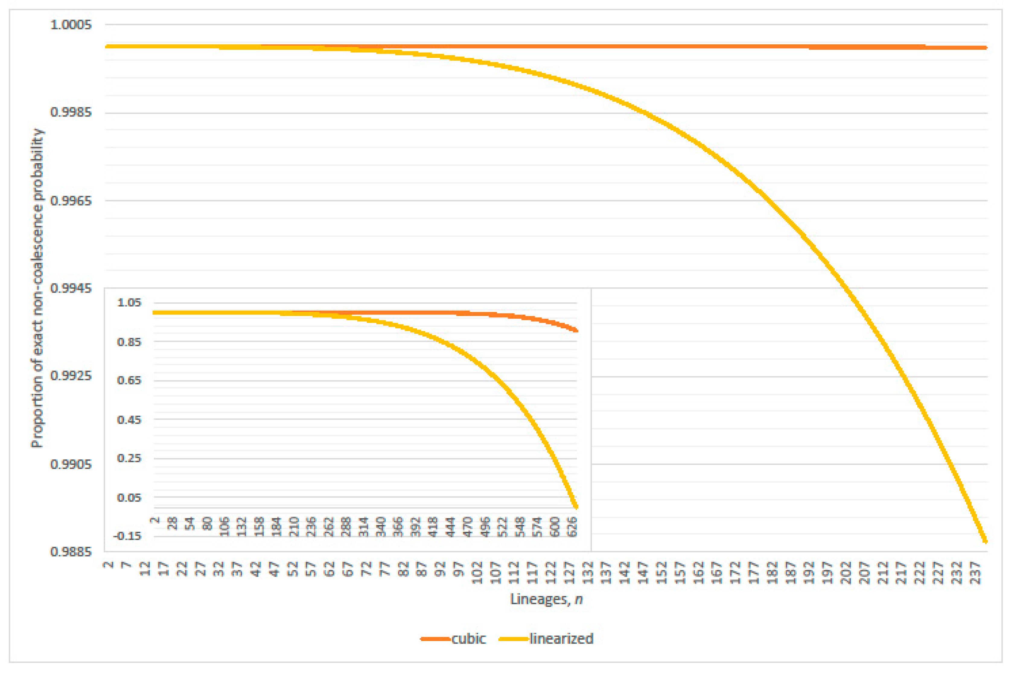
Figure 1. Proportions of the exact non-coalescence probability: quotients of the linearized 1 ( n 2 ) / N and (cubic) third order approximation of Equation (4) upon the exact non-coalescence probability of Equation (1), respectively. Population size N = 2 × 10 5 and n = 2 , , 240 (inset n = 2 , , 633 ) .
Mathematics 06 00082 g001
Figure 2. Proportion of exact non-coalescence probability: quotients of the linearized 1 ( n 2 ) / N , (quadratic) second order and (cubic) third order approximation of Equation (4) upon the exact non-coalescence probability of Equation (1), respectively. Population size N = 2 × 10 5 and n = 2 , , 500 (inset n = 2 , , 240 ).
Mathematics 06 00082 g002
Figure 3. Non-coalescence probabilities: exact Equation (1), linearized 1 ( n 2 ) / N , (quadratic) second order and (cubic) third order approximation of Equation (4), respectively. Population size N = 2 × 10 5 and n = 2 , , 500 (inset n = 2 , , 100 ) .
Mathematics 06 00082 g003
Figure 4. Quadratic term given by Equation (5) minus cubic term given by Equation (6) of Equation (4), and exact Equation (1) minus linearized 1 ( n 2 ) / N non-coalescence probabilities. Population size N = 2 × 10 5 and n = 2 , , 633 (inset n = 2 , , 50 ).
Mathematics 06 00082 g004
Figure 5. Quotients of linearized upon exact probabilities: (i) linearized ( n 2 ) / N upon exact Equation (1) non-coalescence probability; (ii) linearized coalescence ( n 2 ) / N upon exact at least one coalescence probability (complimentary event of Equation (1)); and (iii) linearized coalescence ( n 2 ) / N upon the exact single-pair coalescence probability of Equation (7). Population size N = 2 × 10 5 and n = 2 , , 250 (inset n = 2 , , 50 ).
Mathematics 06 00082 g005
Figure 6. Absolute errors types I and II, inset relative errors types I and II; per generation, n = 2 , , 50 . Population size N = 2 × 10 5 .
Mathematics 06 00082 g006
Figure 7. Absolute error types I and II, inset relative error types I and II; per generation, n = 2 , , 500 . Population size N = 2 × 10 5 .
Mathematics 06 00082 g007
Figure 8. Minmax phase transition by comparison of relative errors; type I upon type II, per generation. Population size N = 2 × 10 5 and n = 2 , , 500 .
Mathematics 06 00082 g008
Figure 9. Exact coalescence probability: at least one coalescence (complimentary event of Equation (1)), single-pair (Equation (7)), double-pair (Equation (8)) and triple-pair (Equation (10)) coalescence probabilities. Population size N = 2 × 10 5 and n = 2 , , 500 (inset n = 2 , , 50 ) .
Mathematics 06 00082 g009
Figure 10. Conditional probabilities of double-pair (Equation (8)), triple-pair (Equation (10)), and triplet (Equation (9)) given either linearized coalescence ( n 2 ) / N or exact at least one coalescence (complimentary event of Equation (1)), respectively; N = 2 × 10 5 and n = 2 , , 500 (inset n = 2 , , 50 ).
Mathematics 06 00082 g010
Figure 11. Exact conditional probabilities of single-pair (Equation (7)) and double-pair (Equation (8)) coalescence given the event of at least one coalescence (compliment of Equation (1)), respectively. Percentage of expected cumulative total genealogical inter-arrival generations shows significance of expected interval durations with n lineages present. Population size N = 2 × 10 5 and n = 2 , , 500 (inset n = 2 , , 50 ).
Mathematics 06 00082 g011
Figure 12. Exact conditional probabilities of single-pair (Equation (7)) and double-pair (Equation (8)) coalescence given the event of at least one coalescence (complimentary event of Equation (1)), respectively. Percentage of expected cumulative total genealogical inter-arrival generations shows the significance of expected interval durations with n lineages present. Population size N = 2 × 10 4 and n = 2 , , 200 (inset n = 2 , , 30 ).
Mathematics 06 00082 g012
Figure 13. Exact conditional probabilities of single-pair (Equation (7)) and double-pair (Equation (8)) coalescence given the event of at least one coalescence (complimentary event to Equation (1)), respectively. Percentage of expected cumulative total genealogical inter-arrival generations shows significance of expected interval durations with n lineages present. Population size N = 2 × 10 6 and n = 2 , 3 . , 1200 (inset n = 2 , 3 . , 300 ) .
Mathematics 06 00082 g013
Figure 14. Exact conditional multi-coalescence probabilities given the event of at least one coalescence (complimentary event of Equation (1)); double-pair (Equation (8)), triplet (Equation (9)), triple-pair (Equation (10)), single-pair with triplet (Equation (11)), and quadruplet (Equation (12)) coalescence. Population size N = 2 × 10 5 and n = 3 , , 100 .
Mathematics 06 00082 g014
Figure 15. Exact conditional multi-coalescence probabilities given the event of at least one coalescence (complimentary event of Equation (1)); double-pair (Equation (8)), triplet (Equation (9)), triple-pair (Equation (10)), single-pair with triplet (Equation (11)), and quadruplet (Equation (12)) coalescence. Population size N = 2 × 10 4 and n = 3 , , 100 .
Mathematics 06 00082 g015
Figure 16. Exact conditional multi-coalescence probabilities given the event of at least one coalescence (complimentary event of Equation (1)); double-pair (Equation (8)), triplet (Equation (9)), triple-pair (Equation (10)), single-pair with triplet (Equation (11)), and quadruplet (Equation (12)) coalescence. Population size N = 2 × 10 6 and n = 3 , , 300 .
Mathematics 06 00082 g016
Figure 17. Quotient of single-pair coalescence probability upon double-pair coalescence probability. Evaluation of Equation (13) as lineages n vary; population sizes N = 2 × 10 4 , 2 × 10 5 , 2 × 10 6 and n = 3 , 4 , , 500 . Percentage of expected cumulative total genealogical inter-arrival generations shows significance of expected interval durations with n lineages present, the case n = 2 omitted (equals one).
Mathematics 06 00082 g017
Figure 18. Logarithm base 10 of expected inter-arrival generations obtained from the reciprocals of single-pair (Equation (7)) and double-pair (Equation (8)) exact coalescence probabilities. Population size N = 2 × 10 5 and n = 2 , 3 , , 500 (inset n = 2 , 3 , , 50 ). Due to a property of the Wright-Fisher model such that a geometric distribution determines the number of generations until a coalescence event occurs, the success probability of the distribution equals either Equation (7) or Equation (8).
Mathematics 06 00082 g018
Figure 19. Parity, per expected interval, restricted Wright-Fisher models: inclusively expanded set of ancestral transitions; single-pair, double-pair, triplet, decrement of three (comprises triple-pair, single-pair with triplet, and quadruplet). Normalized curve accords with Equation (17) of the Kingman coalescent. Population size N = 2 × 10 5 and n = 2 , 3 , , 500 (inset n = 2 , 3 , , 100 ).
Mathematics 06 00082 g019
Figure 20. Expected genealogical parity, restricted Wright-Fisher models, inclusively expanded set of ancestral transitions; single-pair, double-pair, triplet, decrement of three (comprises triple-pair, single-pair with triplet, and quadruplet). Normalized curve accords with Equation (17) of the Kingman coalescent. Population size N = 2 × 10 5 and n = 2 , 3 , , 500 (inset n = 2 , 3 , , 100 ).
Mathematics 06 00082 g020
Figure 21. Corresponds to Figure 19 with population size reduced ten-fold. Parity, per expected interval, restricted Wright-Fisher models: inclusively expanded set of ancestral transitions; single-pair, double-pair, triplet, decrement of three (comprises triple-pair, single-pair with triplet, and quadruplet). Normalized curve accords with Equation (17) of the Kingman coalescent. Population size N = 2 × 10 4 and n = 2 , 3 , , 200 (inset n = 2 , 3 , , 40 ).
Mathematics 06 00082 g021
Figure 22. Corresponds to Figure 20 with population size reduced ten-fold. Expected genealogical parity, restricted Wright-Fisher models, inclusively expanded set of ancestral transitions; single-pair, double-pair, triplet, decrements of three (comprises triple-pair, single-pair with triplet, and quadruplet). Normalized curve accords with Equation (17) of the Kingman coalescent. Population size N = 2 × 10 4 and n = 2 , 3 , , 200 (inset n = 2 , 3 , , 40 ).
Mathematics 06 00082 g022
Figure 23. Corresponds to Figure 19 with population size enlarged ten-fold. Parity, per expected interval, restricted Wright-Fisher models: inclusively expanded set of ancestral transitions; single-pair, double-pair, triplet, decrement of three (comprises triple-pair, single-pair with triplet, and quadruplet). Normalized curve accords with Equation (17) of the Kingman coalescent. Population size N = 2 × 10 6 and n = 2 , 3 , , 1200 (inset n = 2 , 3 , , 300 ).
Mathematics 06 00082 g023
Figure 24. Corresponds to Figure 20 with population size enlarged ten-fold. Expected genealogical parity, restricted Wright-Fisher models, inclusively expanded set of ancestral transitions; single-pair, double-pair, triplet, decrements of three (comprises triple-pair, single-pair with triplet, and quadruplet). Normalized curve accords with Equation (17) of the Kingman coalescent. Population size N = 2 × 10 6 and n = 2 , 3 , , 1200 (inset n = 2 , 3 , , 300 ).
Mathematics 06 00082 g024
Table 1. Percentage overestimation of linearized coalescence probability reached at n lineages.
N 1 % 5 % 10 % 15 % 20 % 25 %
2 × 10 4 30 64 90 109 124 138
2 × 10 6 284 629 882 1072 1229 1364
Table 2. Restricted Wright-Fisher models; column headings describe inclusively expanded sets of ancestral transitions. Maximum lineages n such that parity, per expected interval, exceeds 99%.
Population Size, NSingle-PairDouble-PairTripletDecrements of Three
200010293452
20,0003098102164
200,00091316319516
2,000,000284100210041633
20,000,000895317431785159