Economic Model Predictive Control with Zone Tracking


Abstract
:1. Introduction
2. Problem Setup
2.1. Notation
2.2. System Description and Control Objective
3. EMPC with Zone Tracking
3.1. EMPC Formulation
3.2. Stability Analysis
3.3. Prioritized Zone Tracking
4. Modified Target Zone
| Algorithm 1: Modified target zone. | |
| 1. | Choose some and |
| 2. | Set |
| 3. | for |
| Calculate with Equation. (20) | |
| end | |
| 4. | The modified target zone is |
- (i)
- If is an exact zone tracking penalty for for all , then the modified target zone is forward invariant under the closed-loop system. That is,
- (ii)
- If in addition Assumptions 1 and 2 hold, the transient economic performance in the modified target zone is upper bounded such that for any time instant K where , the following holds:
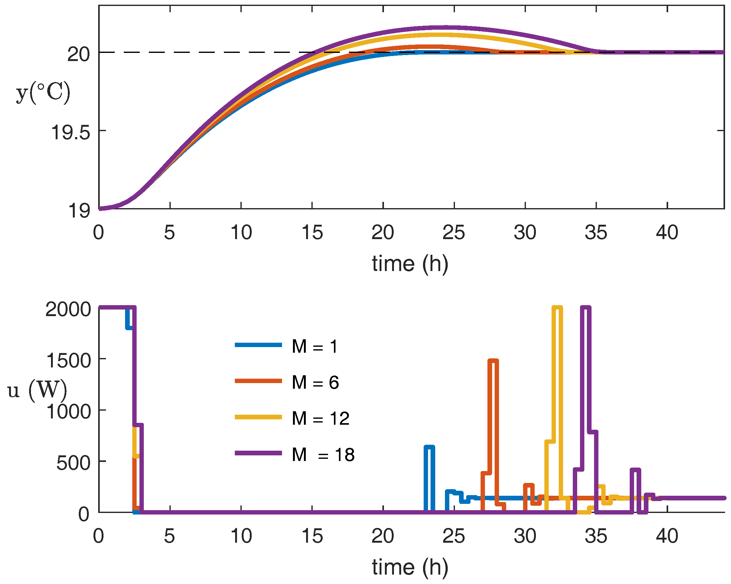
5. Simulation
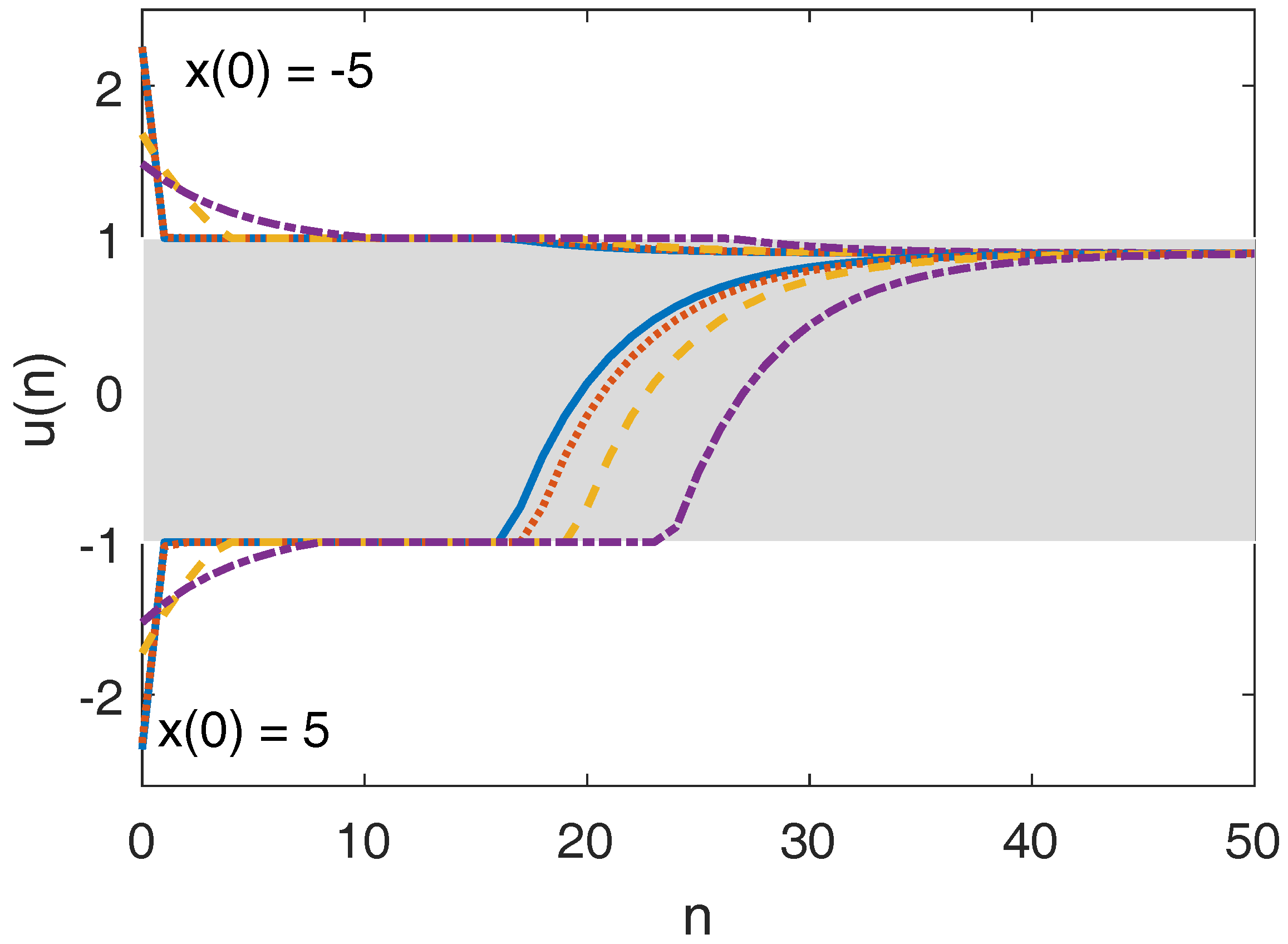
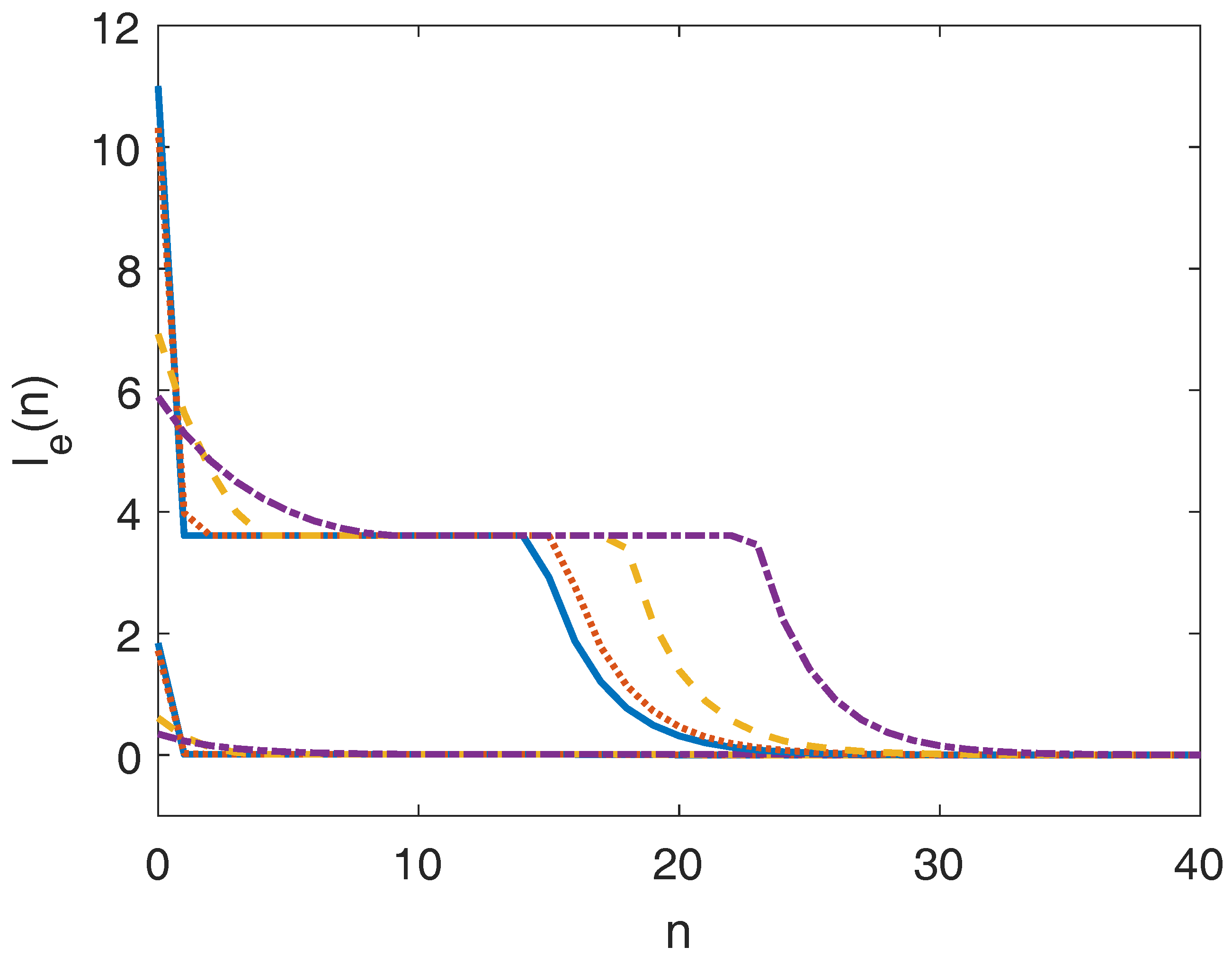
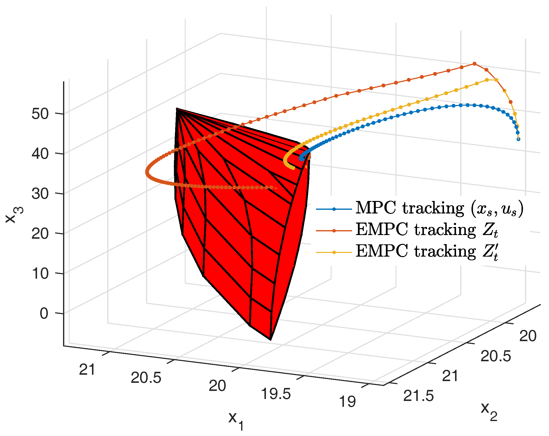
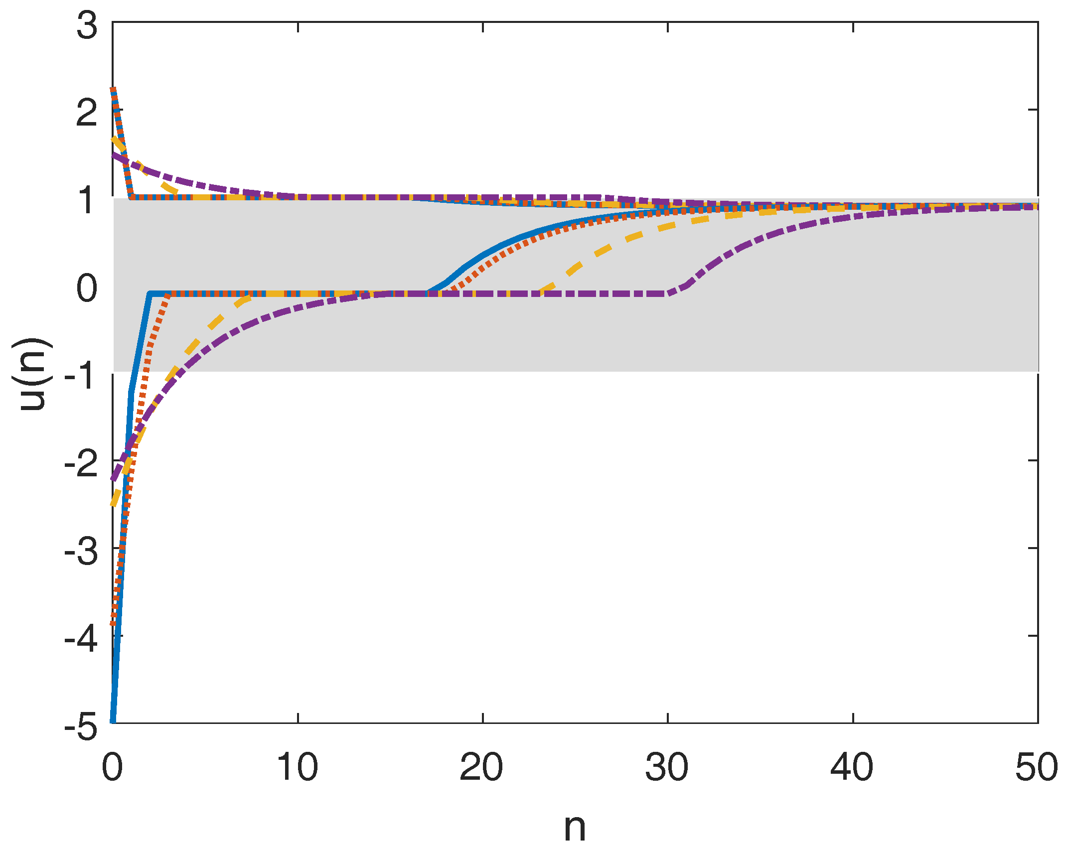
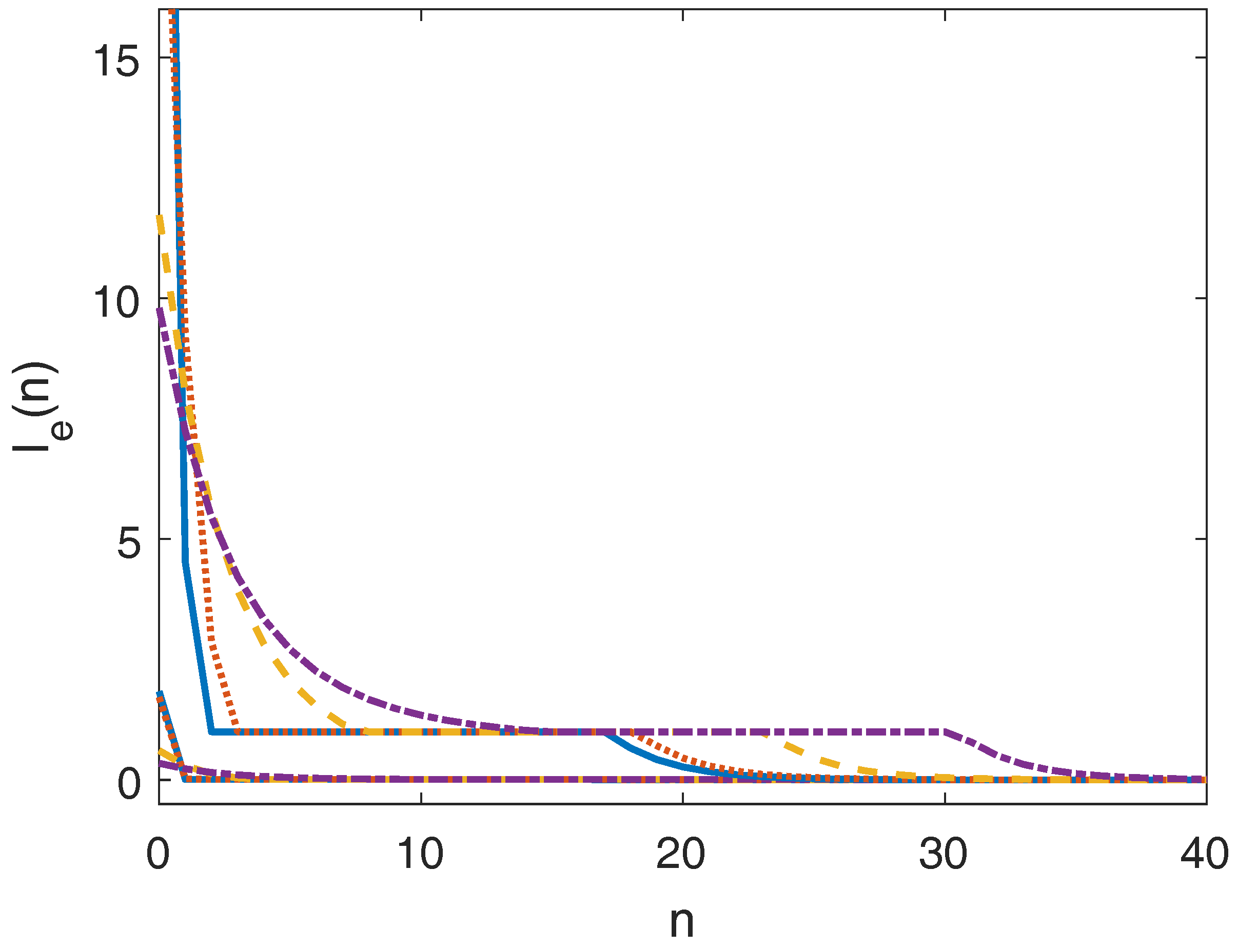
5.1. Example 1
5.1.1. EMPC Tracking the Original Target Zone
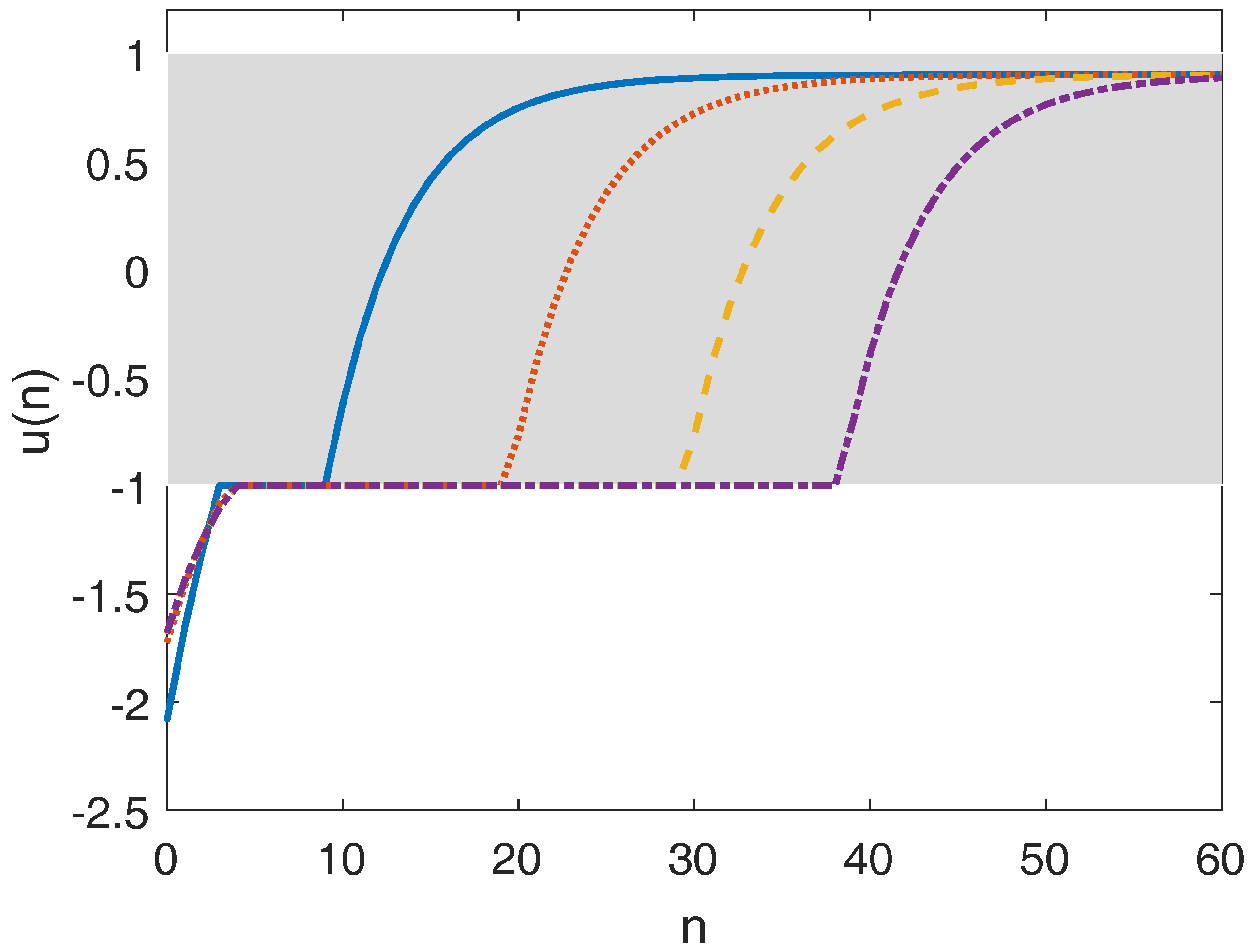
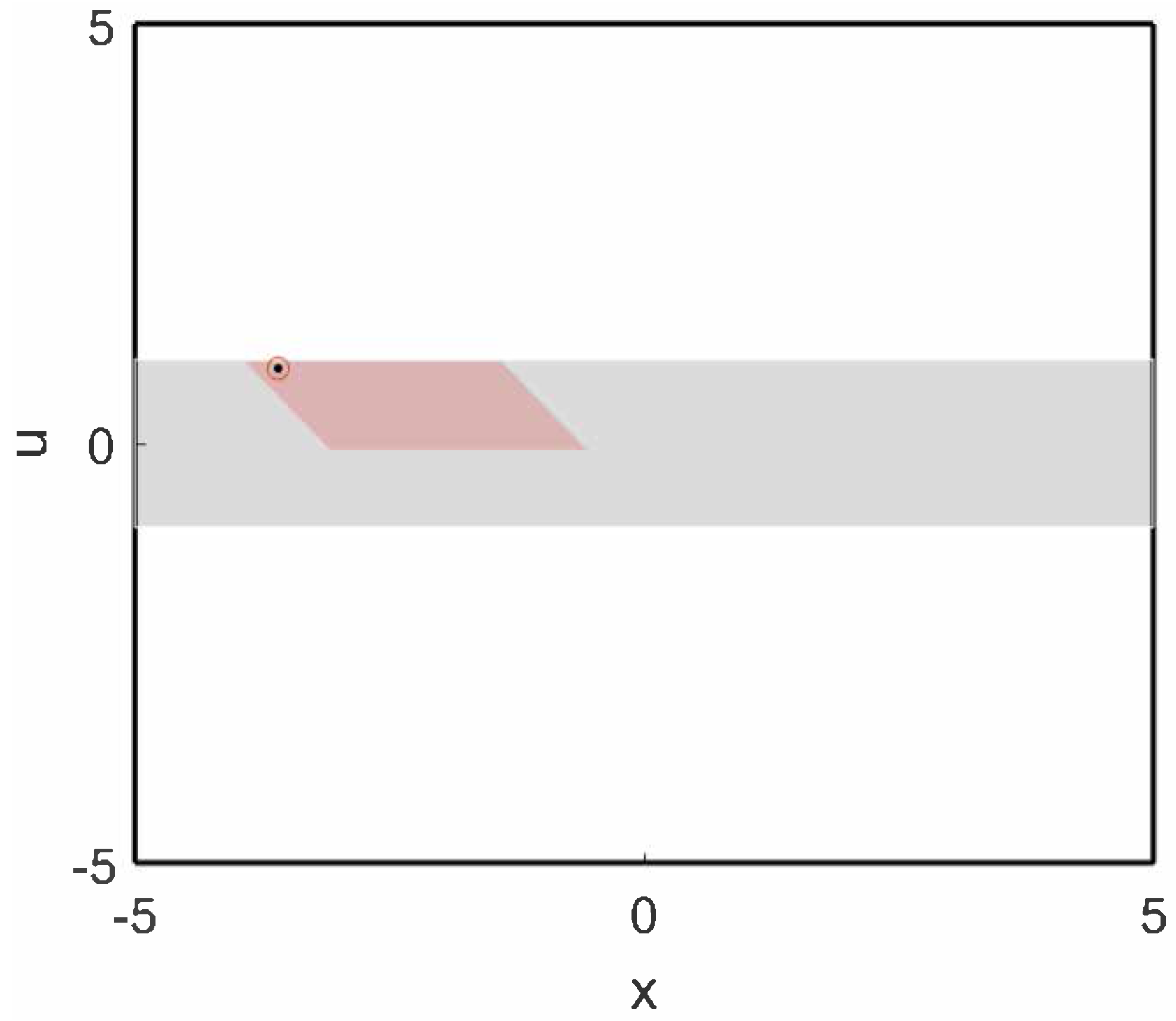
5.1.2. EMPC Tracking the Modified Target Zone
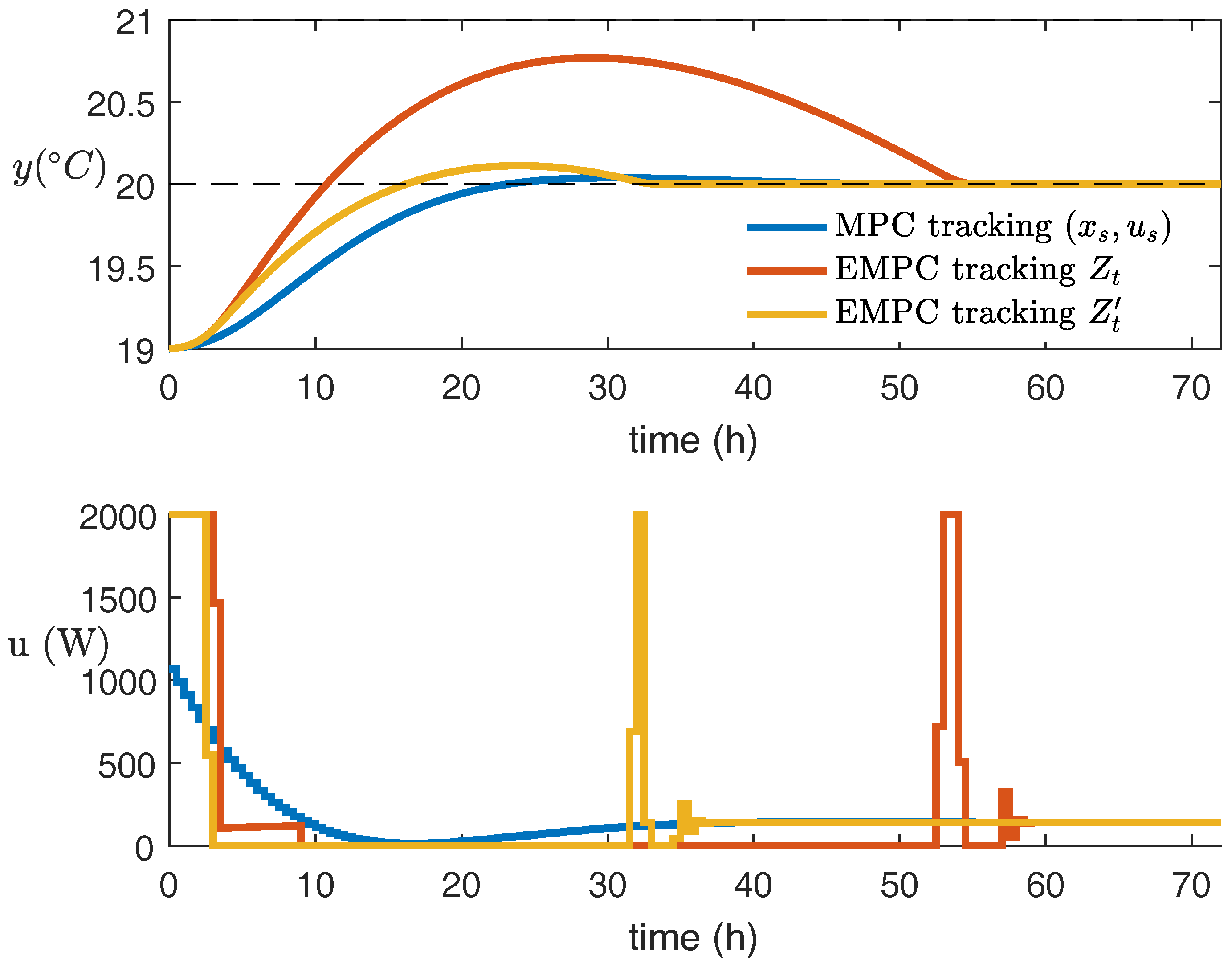
5.2. Example 2
6. Conclusions
Author Contributions
Conflicts of Interest
References
- Lu, J.Z. Challenging control problems and emerging technologies in enterprise optimization. Control Eng. Pract. 2003, 11, 847–858. [Google Scholar] [CrossRef]
- Mayne, D.Q.; Rawlings, J.B.; Rao, C.V.; Scokaert, P.O.M. Constrained model predictive control: Stability and optimality. Automatica 2000, 36, 789–814. [Google Scholar] [CrossRef]
- Rawlings, J.B.; Angeli, D.; Bates, C.N. Fundamentals of economic model predictive control. In Proceedings of the 51th IEEE Conference on Decision and Control, Grand Wailea, HI, USA, 10–13 December 2012; pp. 3851–3861. [Google Scholar]
- Grüne, L. Economic receding horizon control without terminal constraints. Automatica 2013, 49, 725–734. [Google Scholar] [CrossRef]
- Ellis, M.; Durand, H.; Christofides, P.D. A tutorial review of economic model predictive control methods. J. Process Control 2014, 24, 1156–1178. [Google Scholar] [CrossRef]
- Liu, S.; Liu, J. Economic model predictive control with extended horizon. Automatica 2016, 73, 180–192. [Google Scholar] [CrossRef]
- Scokaert, P.; Rawlings, J.B. Feasibility issues in linear model predictive control. AIChE J. 1999, 45, 1649–1659. [Google Scholar] [CrossRef]
- Kerrigan, E.C.; Maciejowski, J.M. Soft constraints and exact penalty functions in model predictive control. In Proceedings of the UKACC International Conference Control, Cambridge, UK, 4–7 October 2000. [Google Scholar]
- De Oliveira, N.M.C.; Biegler, L.T. Constraint handing and stability properties of model-predictive control. AIChE J. 1994, 40, 1138–1155. [Google Scholar] [CrossRef]
- Zeilinger, M.N.; Morari, M.; Jones, C.N. Soft Constrained Model Predictive Control With Robust Stability Guarantees. IEEE Trans. Autom. Control 2014, 59, 1190–1202. [Google Scholar] [CrossRef]
- Askari, M.; Moghavvemi, M.; Almurib, H.A.F.; Haidar, A.M.A. Stability of Soft-Constrained Finite Horizon Model Predictive Control. IEEE Trans. Ind. Appl. 2017, 53, 5883–5892. [Google Scholar] [CrossRef]
- Ferramosca, A.; Limon, D.; González, A.H.; Odloak, D.; Camacho, E. MPC for tracking zone regions. J. Process Control 2010, 20, 506–516. [Google Scholar] [CrossRef]
- Lez, A.H.G.; Marchetti, J.L.; Odloak, D. Robust model predictive control with zone control. IET Control Theory Appl. 2009, 3, 121–135. [Google Scholar]
- González, A.H.; Odloak, D. A stable MPC with zone control. J. Process Control 2009, 19, 110–122. [Google Scholar] [CrossRef]
- Blanchini, F. Set invariance in control. Automatica 1999, 35, 1747–1767. [Google Scholar] [CrossRef]
- Amrit, R.; Rawlings, J.B.; Angeli, D. Economic optimization using model predictive control with a terminal cost. Annu. Rev. Control 2011, 35, 178–186. [Google Scholar] [CrossRef]
- Diehl, M.; Amrit, R.; Rawlings, J.B. A Lyapunov function for economic optimizing model predictive control. IEEE Trans. Autom. Control 2011, 56, 703–707. [Google Scholar] [CrossRef]
- Rao, C.V.; Rawlings, J.B. Linear programming and model predictive control. J. Process Control 2000, 10, 283–289. [Google Scholar] [CrossRef]
- Fletcher, R. Practical Methods of Optimization; John Wiley & Sons: New York, NY, USA, 2013. [Google Scholar]
- Kerrigan, E.C.; Maciejowski, J.M. Invariant sets for constrained nonlinear discrete-time systems with application to feasibility in model predictive control. In Proceedings of the 39th IEEE Conference on Decision and Control, Sydney, Australia, 12–15 December 2000; Volume 5, pp. 4951–4956. [Google Scholar]
- Keerthi, S.; Gilbert, E. Computation of minimum-time feedback control laws for discrete-time systems with state-control constraints. IEEE Trans. Autom. Control 1987, 32, 432–435. [Google Scholar] [CrossRef]
- Halvgaard, R.; Poulsen, N.K.; Madsen, H.; Jørgensen, J.B. Economic model predictive control for building climate control in a smart grid. In Proceedings of the IEEE Innovative Smart Grid Technologies, Washington, DC, USA, 16–20 January 2012; pp. 1–6. [Google Scholar]


| 2.0195 | 2.0225 | 1.2560 | 1.2465 | |
| 76.1218 | 79.5542 | 86.5742 | 103.0781 |
| Tracking | ||||
|---|---|---|---|---|
| 2.0195 | 2.0225 | 1.2560 | 1.2465 | |
| 76.1218 | 79.5542 | 86.5742 | 103.0781 | |
| Tracking | ||||
| 2.0195 | 2.0225 | 1.2560 | 1.2465 | |
| 57.4483 | 52.7305 | 54.9608 | 64.2366 |
| Variable | Unit | Description |
|---|---|---|
| °C | Room air temperature | |
| °C | Floor temperature | |
| °C | Water temperature in floor heating pipes | |
| W | Heat pump compressor input power | |
| °C | Ambient temperature | |
| W | Solar radiation power |
| MPC Tracking | EMPC Tracking | EMPC Tracking | |
|---|---|---|---|
| Additional electricity cost (USD) | 363.3 | 411.1 | 369.8 |
© 2018 by the authors. Licensee MDPI, Basel, Switzerland. This article is an open access article distributed under the terms and conditions of the Creative Commons Attribution (CC BY) license (http://creativecommons.org/licenses/by/4.0/).
Share and Cite
Liu, S.; Liu, J. Economic Model Predictive Control with Zone Tracking. Mathematics 2018, 6, 65. https://doi.org/10.3390/math6050065
Liu S, Liu J. Economic Model Predictive Control with Zone Tracking. Mathematics. 2018; 6(5):65. https://doi.org/10.3390/math6050065
Chicago/Turabian StyleLiu, Su, and Jinfeng Liu. 2018. "Economic Model Predictive Control with Zone Tracking" Mathematics 6, no. 5: 65. https://doi.org/10.3390/math6050065
APA StyleLiu, S., & Liu, J. (2018). Economic Model Predictive Control with Zone Tracking. Mathematics, 6(5), 65. https://doi.org/10.3390/math6050065