1. Introduction
Chaotic itinerancy is a concept used to refer to a dynamical behavior in which typical orbits visit a sequence of regions of the phase space called “quasi attractors” or “attractor ruins” in some irregular way. Informally speaking, during this itinerancy, the orbits visit a neighborhood of a quasi attractor (the attractor ruin) with a relatively regular and stable motion, for relatively long times and then the trajectory jumps to another quasi attractor of the system after a relatively small chaotic transient. This behavior was observed in several models and experiments related to the dynamics of neural networks and related to neurosciences (see [
1]). In this itinerancy, the visit near some attractors was associated to the appearance of some macroscopic aspect of the system, like the emergence of a perception or a memory, while the chaotic iterations from a quasi attractor to another are associated to an intelligent (history dependent with trial and errors) search for the next thought or perception (see [
2]). This kind of phenomena was observed in models of the neural behavior which are fast-slow systems or random dynamical systems (sometimes modeling as a random system the fast-slow behavior).
As far as we know the concept did not have a complete mathematical formalization though in [
3] some mathematical scenarios are presented, showing some situations in which these phenomena may appear. Often this phenomenon is associated to the presence of some kind of “weak” attractor, as Milnor type attractors (see e.g., [
3] or [
4]) in the system and to small perturbations allowing typical trajectories to escape the attractor. Chaotic itinerancy was found in many applied contexts, but a systematic treatment of the literature is out of the scope of this paper, for which we invite the reader to consult [
1] for a wider introduction to the subject and to its literature.
In this paper, our goal is to investigate and illustrate this concept from a mathematical point of view with some meaningful examples. We consider a simple one-dimensional random map derived from the literature on the subject (see
Section 3). This map is a relatively simple discrete time random dynamical system on the interval, suggested by the behavior of certain macrovariables in the neural networks studied in [
5], modeling the neocortex with a variant of Hopfield’s asynchronous recurrent neural network presented in [
6]. In Hopfield’s network, memories are represented by stable attractors and an unlearning mechanism is suggested in [
7] to account for unpinning of these states (see also, e.g., [
8]). In the network presented in [
5], however, these are replaced by Milnor attractors, which appear due to a combination of symmetrical and asymmetrical couplings and some resetting mechanism. A similar map is also obtained in [
9], in the context of the BvP neuron driven by a sinusodial external stimulus. They belong to a family known as Arnold circle maps (named after [
10]), which are useful in physiology (see [
11] (Equation (
3))). The simple model we study shares with the more complicated models from which it is derived the presence of quasi attractors (it can be seen as a stochastic perturbation of a system with Milnor attractors), its undestanding can bring some light on the mathematical undestanding of chaotic itinearacy.
The model we consider is made by a deterministic map
T on the circle perturbed by a small additive noise. For a large enough noise, its associated random dynamical system exhibits an everywhere positive stationary density concentrated on a small region (see [
12] for an analytical treatment), which can be attributed to the chaotic itinerancy of the neural network.
In the paper, with the help of a computer aided proof, we establish several results about the statistical and geometrical properties of the above system, with the goal to show that “the behavior of this system exhibits a kind of chaotic itineracy”. We show that the system is (exponentially) mixing, hence globally chaotic. We also show a rigorous estimate of the density of probability (and then the frequency) of visits of typical trajectories near the attractors, showing that this is relatively high with respect to the density of probability of visits in other parts of the space. This is done by a computer aided rigorous estimate of the stationary probability density of the system. The computer aided proof is based on the approximation of the transfer operator of the real system by a finite rank operator which is rigorously computed and whose properties are estimated by the computer. The approximation error from the real system to the finite rank one is then managed using an appropriated functional analytic approach developed in [
13] for random systems (see also [
14,
15,
16] for applications to deterministic dynamics or iterated functions systems).
The paper is structured as follows. In
Section 2, we review basic definitions related to random dynamical systems, in particular, the Perron-Frobenius operator, which will play a major role. In
Section 3, we present our example along with an explanation of the method used to study it. The numerical results supported by the previous theoretical sections are presented in
Section 4, while in
Section 5 we present a conclusion with some additional comments.
2. Random Dynamical Systems
This section follows [
17,
18]. We denote by
a probability space and by
the corresponding space of sequences (over
or
), with the product
-algebra and probability measure. In addition, we denote by
f the shift map on
M,
, where
or
.
Definition 1. Let be a measurable space. Endow with the product σ-algebra . A random transformation
over f is a measurable transformation of the formwhere depends only on the zeroth coordinate of x. Suppose we have a (bounded, measurable) function . Given a random orbit , for which we know the value of , we may ask what is the expected value for , that is, . Since the iterate depends on an outcome , which is distributed according to , this can be calculated as
The equation above defines the
transition operator associated with the random transformation
F as an operator in the space
of bounded measurable functions. Dually, we can consider its
adjoint transition operator (These operators are related by
, for every bounded measurable
(see [
18] (lemma 5.3)).) that acts in the space of probability measures
on
N, defined by
Of particular importance are the fixed points of the operator .
Definition 2. A probability measure η for N is called stationary for the random transformation F if .
We recall the deterministic concept of invariant measures.
Definition 3. If is a measurable mapping in the measurable space , we say ν is an invariant measure for h if for any measurable .
In the one-sided case (), invariant measures and stationary measures for F are related by the following proposition.
Proposition 1 ([
18] (proposition 5.4)).
A probability measure η on N is stationary for F if and only if is invariant for F. Another concept from deterministic dynamical systems that can be naturally extended to random dynamical systems is that of ergodicity.
Definition 4. Suppose η is stationary for F. We say that η is ergodic for F if either
- 1.
every (bounded measurable) function ϕ that is η-stationary, i.e., , is constant in some full η-measure set;
- 2.
every set B that is η-stationary, i.e., whose characteristic function is η-stationary, has full or null η-measure.
In fact, both conditions are equivalent (see [
18] (proposition 5.10)). In the one-sided case, the following proposition relates ergodicity of a random dynamical system with the deterministic concept.
Proposition 2. A stationary measure η is ergodic for F if and only if is an ergodic F-invariant measure.
Suppose N is a manifols with boundary and consider its Lebesgue measure m. It’s useful to consider the measures which are absolutely continuous and the effect of upon their densities. This is possible, for example, if is absolutely continuous for every .
Definition 5. The Perron-Frobenius operator with respect to the random transformation F is the operator (This is an extension to the deterministic case, in which the Koopman operator is used instead of the transition operator.) We can use the Perron-Frobenius operator to define a mixing property.
Proposition 3. We say that a stationary measure is mixing
for F if the Perron-Frobenius operator L satisfiesfor every and (This definition is adapted from [19] (Equation (1.5)).). Since
L and
U are dual, the mixing condition can be restated as
for every
and
, which is similar to the usual definition of decay of correlations.
If
F is mixing, then
F is ergodic for
(see [
17] (Theorem 4.4.1)). In our example, we shall verify the following stronger condition.
Remark 1. It suffices to verify that for some , because .
Proposition 4. If the Perron-Frobenius operator L of a random dynamical system F satisfies Equation (1), then L admits a unique stationary density h and F is mixing. Proof. because
L is a Markov operator [
17] (Remark 3.2.2). Take a density
. We claim that
for some density
h. On the contrary, there would be
and a subsequence
such that
because is a density, and for every , a contradiction.
h is stationary because L is bounded, and unique because implies for any density g. Similarly, the mixing property follows from . ☐
Remark 2. Any density f must converge exponentially fast to the stationary density h. Precisely, given N and such that , the fact that implies that for some and .
In the following, we will use Equation (
1) as the definition of mixing property.
3. A Neuroscientifically Motivated Example
In [
5], a neural network showing successive memory recall without instruction, inspired by Hopfield’s asynchronous neural network and the structure of the mammalian neocortex, is presented.
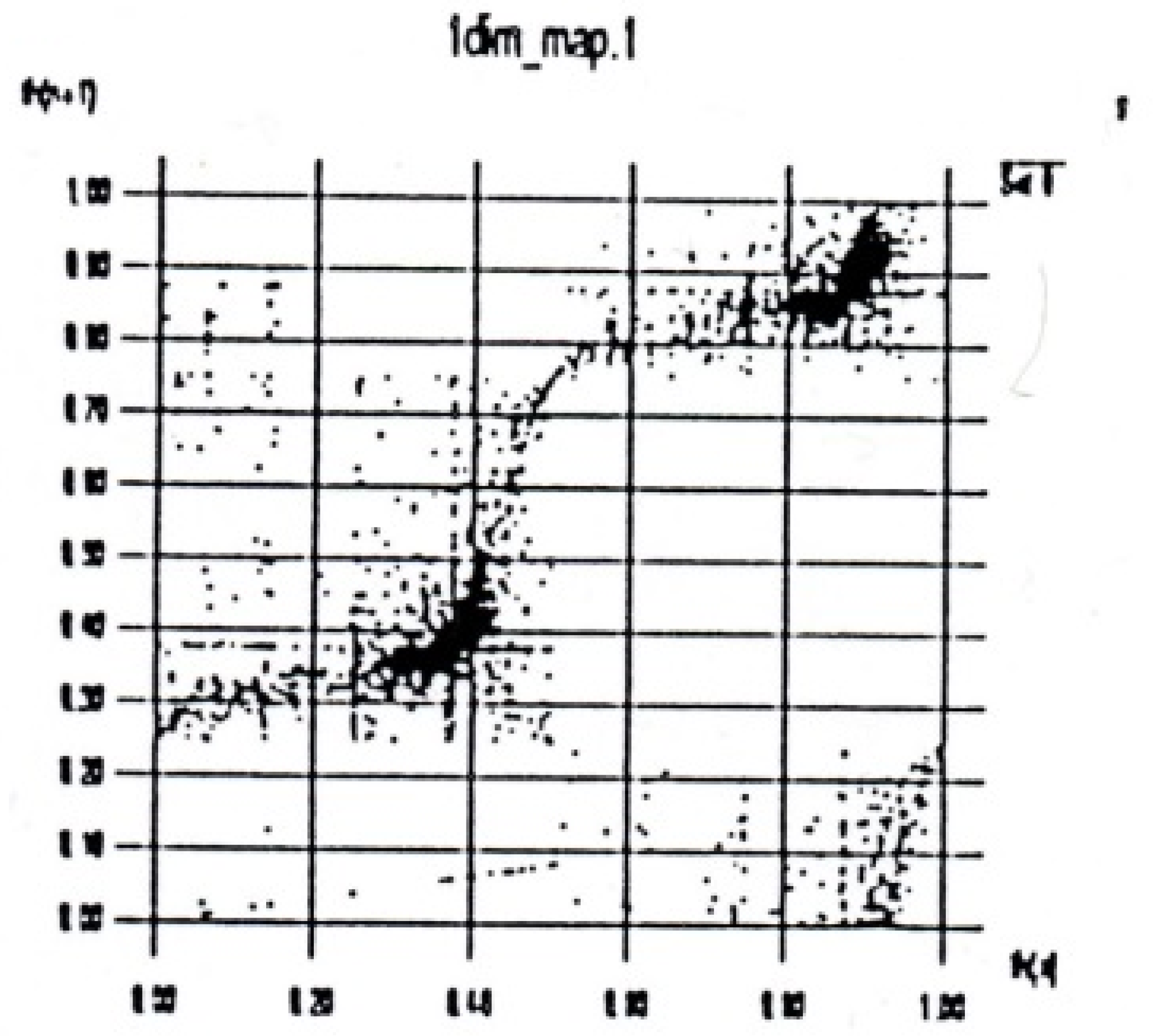
A macrovariable, related to the “activity” of the network (see
Figure 1, similar plots appeared also in [
5,
20]) was observed to evolve as a noisy one dimensional map in the case that the network receives no external stimulus (its definition of can be found in [
5] (p. 6).). This was regarded in [
20] as related to a rule of successive association of memory, exhibiting chaotic dynamics.
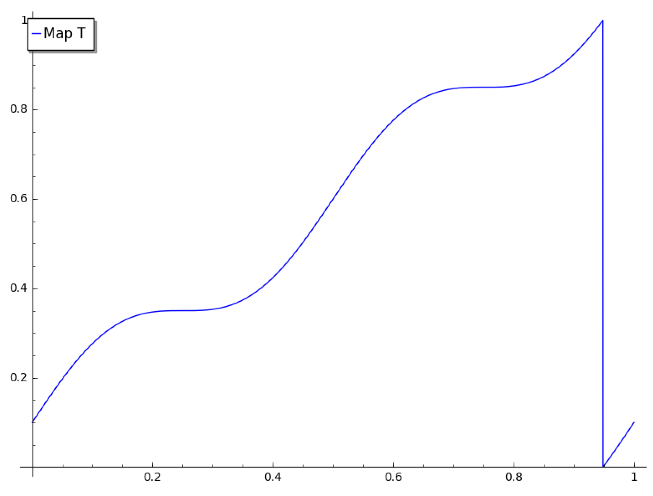
This behavior can be modeled as a random dynamical system
, with a deterministic component given by an Arnold circle map (see
Figure 2) and a stochastic part given by a random additive noise. The system can be hence defined as
for
,
and
an i.i.d. sequence of random variables with a distribution assumed uniform over
.
The Perron-Frobenius operator (Definition 5) associated to this system is given by
(a proof can be found in [
17] (p. 327)), where
is a convolution operator (Equation (
3)) and
L is the Perron-Frobenius operator of
T.
It is well known that such an operator has an invariant probability density in . In the following, we show that can be rigorously approximated and a mixing property can be proved using the numerical estimates.
In addition, a rigorous approximation of the stationary density of is obtained, from which we can conclude the existence of a kind of chaotic itinerancy.
Rigorous Approximation
Here we show how we can study the behavior of the Perron-Frobenius operator associated to Equation (
2) by approximating it by a finite rank operator. The finite rank approximation we use is known in literature as Ulam’s method. For more details, see [
13].
Suppose we are given a partition of
into intervals
and denote the characteristic function of
by
. An operator
can be discretized by
where
is the projection
This operator is completely determined by its restriction to the subspace generated by , and thus may be represented by a matrix in this base, which we call the Ulam matrix. In the following, we assume that and is a partition of with diameter .
For computational purposes, the operator is discretized as
This is simple to work with because it is the product of the discretized operators and .
Let
and denote by
and
the stationary probability densities for
and
, respectively. Suppose
for some
. Since
and ([
13] (Equation (
2)))
we search a good estimate of
to prove both mixing of
and give a rigorous estimate of
.
Since the calculus of
is computationally complex, an alternative approach is used in [
13] (see [
22] for a previous application of a similar idea to deterministic dynamics). First, we use a coarser version of the operator,
, where
is a multiple of
. Then, we determine
and constants
, for
, and
in order that
Finally, the following lemma from [
13] is used.
Lemma 1. Let ; let σ be a linear operator such that , , and ; let . Then we have It is applied to two cases.
,
and
implies
This is used to obtain
,
and
, such that
,
and
implies
By Remark 1, we conclude that the mixing condition is satisfied whenever
We remark that a simple estimate to Equation (
5) is given by ([
13] (Equation (
4)))
The analysis of data obtained from the numerical approximation
of
, in particular its variance, allows the algorithm in [
13] to improve greatly this bound, using interval arithmetic. In
Table 1, the value
l1apriori obtained from the first estimate Equation (
9) and the best estimate
l1err are compared.
4. Results
We verified mixing and calculated the stationary density for the one dimensional system Equation (
2) using the numerical tools from the
compinv-meas project (see [
13]), which implements the ideas presented in
Section 3.1. The data obtained is summarized in
Table 1.
For an explanation of the values calculated, refer to
Section 3.1. In the column
l1apriori, we have the estimate Equation (
9) for the approximation error of the stationary density in
and in
l1err, the improved estimate as in [
13] (Section 3.2.5).
In every case, we used the following sizes of the partition.
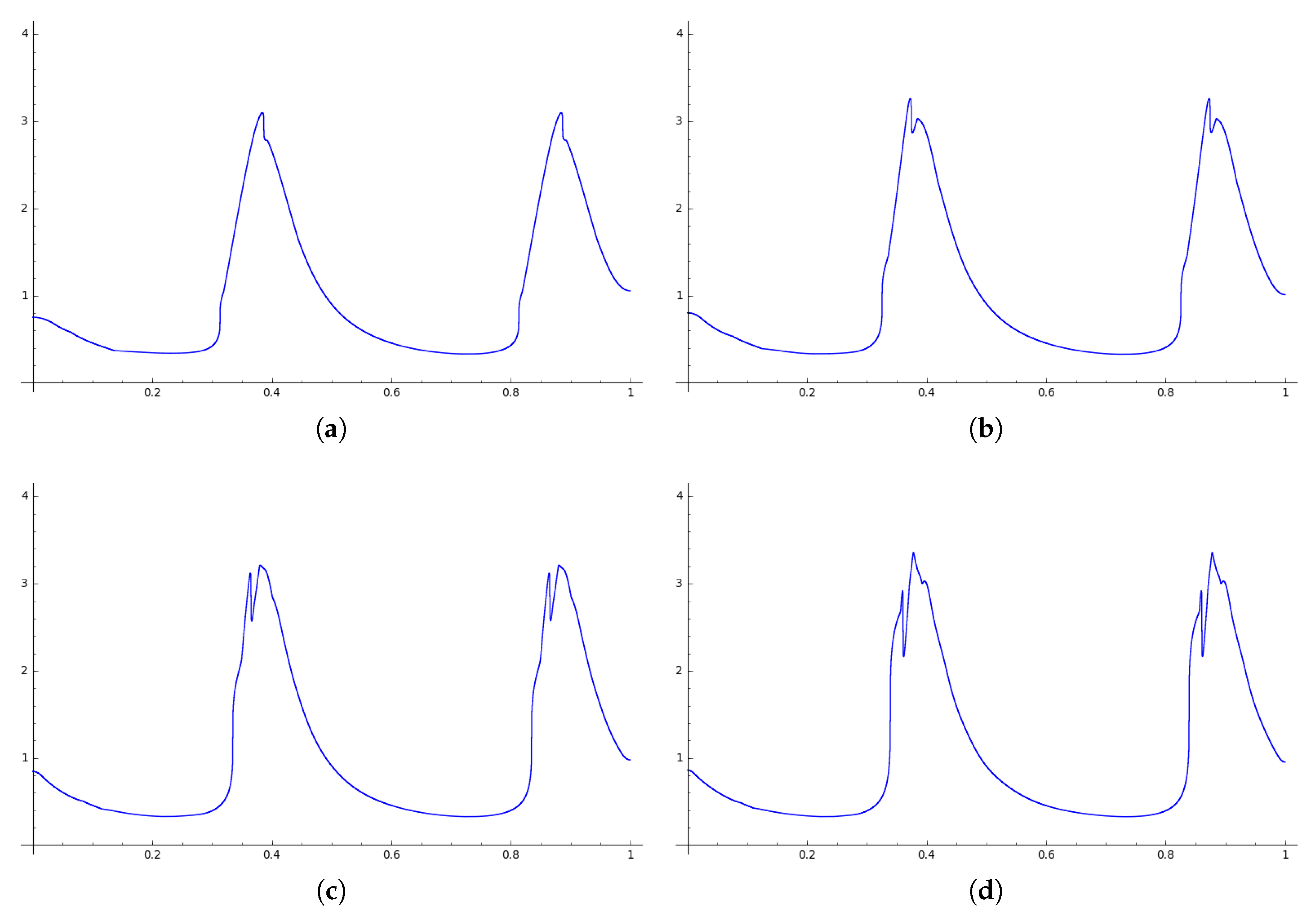
In
Figure 3, stationary densities obtained with this method are shown.
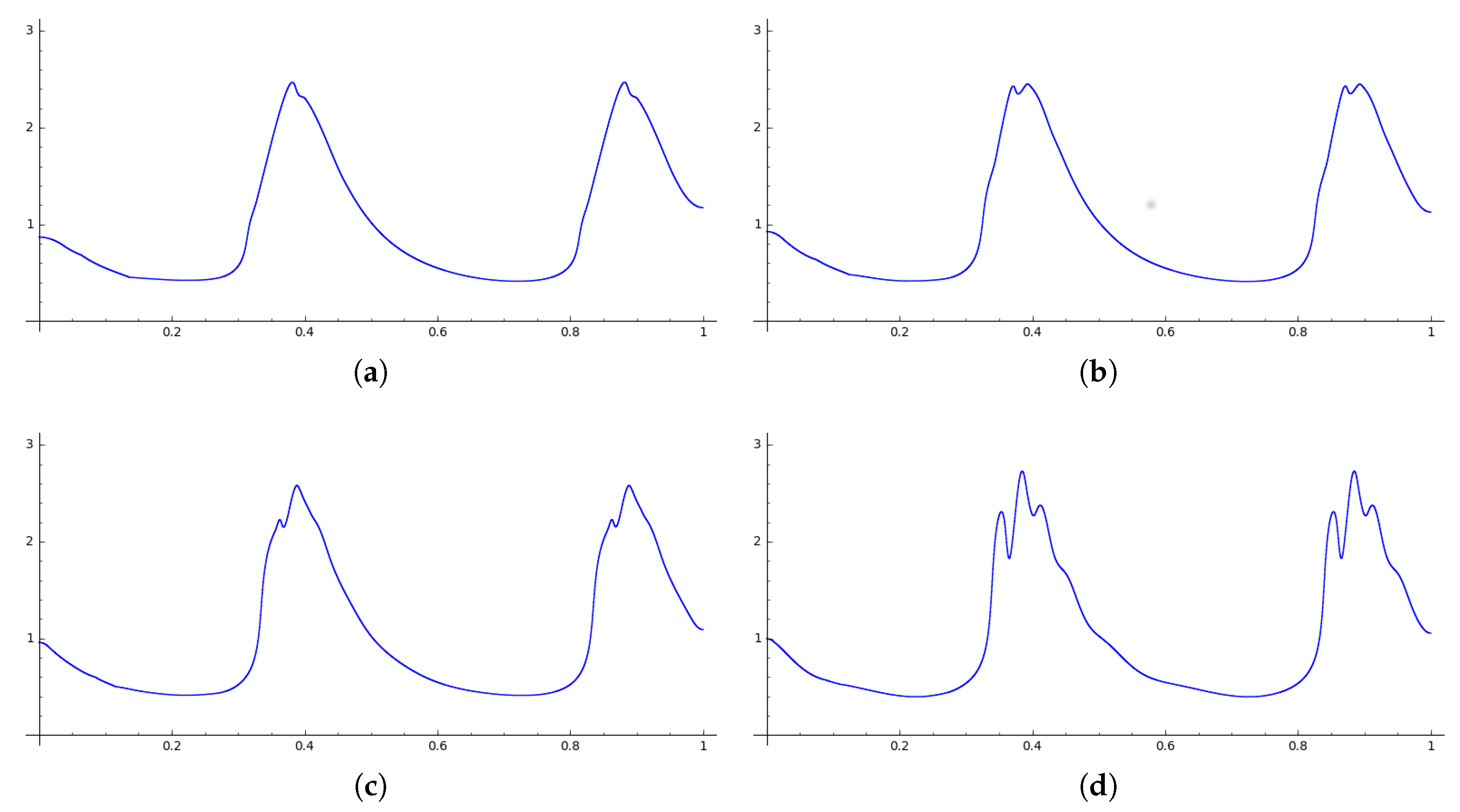
We also studied the system Equation (
2) in the case that
for the same range of noises (
Table 2). In
Figure 4, stationary densities obtained in this case are shown. We note that the same kind of “chaotic itinerancy” obtained in the main case is observed.
5. Conclusions
We have shown how the numerical approach developed in [
13] can be used to study dynamical properties for a one dimensional random dynamical system of interest in the areas of physiology and neural networks.
In particular, we established mixing of the system and a rigorous estimate of its stationary density, which allowed us to observe that the trajectories concentrate in certain “weakly attracting” and “low chaotic” regions of the space, in concordance with the concept of chaotic itinerancy. The concept itself still did not have a complete mathematical formalization, and deeper understanding of the systems where it was found is important to extract its characterizing mathematical aspects.
The work we have done is only preliminary, to obtain some initial rigorous evidence of the chaotic itineracy in the system. Further investigations are important to understand the phenomenon more deeply. Firstly, it would be important to understand more precisely the nature of the phenomenon: rigorously computing Lyapunov exponents and other chaos indicators. It would also be important to investigate the robustness of the behavior of the system under various kinds of perturbations, including the zero noise limit. Another important direction is to refine the model to adapt it better to the experimental data shown in
Figure 1, with a noise intensity which depends on the point.


