Numerical Methods for Solving Fuzzy Linear Systems

Abstract

In this article, three numerical iterative schemes, namely: Jacobi, Gauss–Seidel and Successive over-relaxation (SOR) have been proposed to solve a fuzzy system of linear equations (FSLEs). The convergence properties of these iterative schemes have been discussed. To display the validity of these iterative schemes, an illustrative example with known exact solution is considered. Numerical results show that the SOR iterative method with $\omega =1.3$ provides more efficient results in comparison with other iterative techniques.

1. Introduction

The subject of Fuzzy System of Linear Equations (FSLEs) with a crisp real coefficient matrix and with a vector of fuzzy triangular numbers on the right-hand side arise in many branches of science and technology such as economics, statistics, telecommunications, image processing, physics and even social sciences. In 1965, Zadeh [1] introduced and investigated the concept of fuzzy numbers that can be used to generalize crisp mathematical concept to fuzzy sets.

There is a vast literature on the investigation of solutions for fuzzy linear systems. Early work in the literature deals with linear equation systems whose coefficient matrix is crisp and the right hand vector is fuzzy. That is known as FSLEs and was first proposed by Friedman et al. [2]. For computing a solution, they used the embedding method and replaced the original fuzzy $n\times n$ linear system by a $2n\times 2n$ crisp linear system. Later, several authors studied FSLEs. Allahviranloo [3,4] used the Jacobi, Gauss–Seidel and Successive over-relaxation (SOR) iterative techniques to solve FSLEs. Dehghan and Hashemi [5] investigated the existence of a solution provided that the coefficient matrix is strictly diagonally dominant matrix with positive diagonal entries and then applied several iterative methods for solving FSLEs. Ezzati [6] developed a new method for solving FSLEs by using embedding method and replaced an $n\times n$ FSLEs by two $n\times n$ crisp linear system. Furthermore, Muzziolia et al. [7] discussed FSLEs in the form of $A_{1}x +b_1 = A_{2}x + b_2$ with $A_1$, $A_2$ being square matrices of fuzzy coefficients and $b_1$, $b_2$ fuzzy number vectors. Abbasbandy and Jafarian [8] proposed the steepest descent method for solving FSLEs. Ineirat [9] investigated the numerical handling of the fuzzy linear system of equations (FSLEs) and fully fuzzy linear system of equations (FFSLEs).

Generally, FSLEs is handled under two main headings: square $\left(n\times n\right)$ and nonsquare $\left(m\times n\right)$ forms. Most of the works in the literature dealwith square form. For example, Asady et al. [10], extended the model of Friedman for $n\times n$ fuzzy linear system to solve general $m\times n$ rectangular fuzzy linear system for $\times n$, where the coefficients matrix is crisp and the right-hand side column is a fuzzy number vector. They replaced the original fuzzy linear system $m\times n$ by a crisp linear system $2m\times 2n$. Moreover, they investigated the conditions for the existence of a fuzzy solution.

Fuzzy elements of this system can be taken as triangular, trapezoidal or generalized fuzzy numbers in general or parametric form. While triangular fuzzy numbers are widely used in earlier works, trapezoidal fuzzy numbers have neglected for along time. Besides, there exist lots of works using the parametric and level cut representation of fuzzy numbers.

The paper is organized as follows: In Section 2, a fuzzy linear system of equations is introduced. In Section 3, we present the Jacobi, Gauss–Seidel and SOR iterative methods for solving FSLEs with convergence theorems. The proposed algorithms are implemented using a numerical example with known exact solutions in Section 4. Conclusions are drawn in Section 5.

2. Fuzzy Linear System

Definition 1.

In Reference [11]: An arbitrary fuzzy number in parametric form is represented by an ordered pair of functions $(\overline{v\left(r\right)},\underset{\_}{v\left(r\right)}), 0 \le r \le 1,$ which satisfy the following requirements:

(1)

$\underset{\_}{v\left(r\right)}$ is a bounded left-continuous non-decreasing function over $\left[0, 1\right].$

(2)

$\overline{v\left(r\right)}$ is a bounded left-continuous non-increasing function over $\left[0, 1\right]$.

(3)

$\underset{\_}{v\left(r\right)}\le \overline{v\left(r\right)}$; $0 \le r \le 1.$

Definition 2.

In Reference [12]: For arbitrary fuzzy numbers $u$ and $v$the quantity

$$D(u,v)=\underset{0\le r\le 1}{\sup }\left\{\max \left\{\left|\underset{\_}{u^r}-\underset{\_}{v^r}\right|,\left|{\overline{u}}^r-{\overline{v}}^r\right|\right\}\right\}$$

is called the Hausdorff distance between $u$ and $v$.

Definition 3.

In Reference [13]: The $n \times n$ linear system

$$\{\begin{array}{lll}{a}_{11}{x}_1+a_{12}{x}_2+ \dots +& a_{1n}{x}_n& =b_1\\ a_{21}{x}_1+a_{22}{x}_2+ \dots +& a_{2n}{x}_n& =b_2\\ . & . & . . \\ . & . & . . \\ . & . & . . \\ a_{n1}{x}_1+a_{n2}{x}_2+ \dots & +a_{nn}{x}_n& =b_n\end{array}$$

(1)

where the coefficients matrix $A = \left(a_{ij} \right), 1 \le i, j \le n$ is a crisp $n\times n$ matrix and each $b_i\in E^1, 1 \le i \le n$, is fuzzy number, is called FSLEs.

Definition 4.

In Reference [13]: A fuzzy number vector $X = {\left(x_1, x_2, \dots , x_n\right)}^t$ given by $x_i=\left(\underset{\_}{x_i}\left(r\right),\overline{x_i}\left(r\right)\right),1\le i\le n, 0\le r\le 1$ is called (in parametric form) a solution of the FSLEs (1) if

$$\begin{gathered} \underset{\_}{{\displaystyle \sum }_{j=1}^n{a}_{ij}{x}_j}={\displaystyle \sum }_{j=1}^n\underset{\_}{a_{ij}{x}_j} =\underset{\_}{b_i,} \\ \overline{{\displaystyle \sum }_{j=1}^n{a}_{ij}{x}_j}={\displaystyle \sum }_{j=1}^n\overline{a_{ij}{x}_j}=\overline{b_i}. \end{gathered}$$

(2)

Following Friedman [2] we introduce the notations below:

$$x={\left(\underset{\_}{x_1},\underset{\_}{x_2},\dots \underset{\_}{x_n},-\overline{x_1},-\overline{x_2},\dots -\overline{x_n}\right)}^t$$

$$b={\left(\underset{\_}{b_1},\underset{\_}{b_2},\dots \underset{\_}{b_n},-\overline{b_1},\overline{-b_2},\dots -\overline{b_n}\right)}^t$$

$S=\left(s_{ij}\right), 1\le i, j\le 2n, where s_{ij}$ are determined as follows:

$$\begin{gathered} a_{ij}\ge 0\Rightarrow s_{ij}=a_{ij}, s_{i+n,j+n}=a_{ij}, \\ {a}_{ij}<0\Rightarrow s_{i,j+n}=-a_{ij}, s_{i+n,j}=-a_{ij}. \end{gathered}$$

(3)

and any $s_{ij}$ which is not determined by Equation (3) is zero. Using matrix notation, we have

$$SX = b$$

(4)

The structure of $S$ implies that $s_{ij}\ge 0$ and thus

$$S=\left(\begin{array}{c}B C\\ C B\end{array}\right)$$

(5)

where $B$ contains the positive elements of $A , C$ contains the absolute value of the negative elements of $A$ and $A = B -C.$ An example in the work of Friedman [2] shows that the matrix $S$ may be singular even if $A$ is nonsingular.

Theorem 1.

In Reference [2]: The matrix $S$ is nonsingular matrixif and only if the matrices $A = B -C$ and $B +C$ are both nonsingular.

Proof. 

By subtracting the $j$th column of $S$, from its $\left(n+j\right)$th column for $1\le j\le n$ we obtain

$$S=\left(\begin{array}{c}B \\ C \end{array}\begin{array}{c}C\\ B\end{array}\right)\to \left(\begin{array}{c}B \\ C \end{array}\begin{array}{c}C-B\\ B-C\end{array}\right)=S_1.$$

Next, we adding the $\left(n+i\right)\mathrm{th}$row of $S$ to its $i$th row for $1\le i\le n$ then we obtain

$$S_1=\left(\begin{array}{c}B \\ C \end{array}\begin{array}{c}C-B\\ B-C\end{array}\right)\to \left(\begin{array}{c}B+C \\ C \end{array}\begin{array}{c}0\\ B-C\end{array}\right)=S_2.$$

Clearly, $\left|S\right|=\left|S_1\right|=\left|S_2\right|=\left|B+C\right|\left|B-C\right|=\left|B+C\right|\left|A\right|.$

Therefore

$\left|S\right|\ne 0$ if and only if $\left|A\right|\ne 0$ and $\left|B+C\right|\ne 0,$

These concludes the proof. □

Corollary 1.

In Reference [2]: If a crisp linear system does not have a unique solution, the associated fuzzy linear system does not have one either.

Definition 5.

In Reference [14]: If $X={\left(\underset{\_}{x_1},\underset{\_}{x_2},\dots \underset{\_}{x_n},-\overline{x_1},-\overline{x_2},\dots ,-\overline{x_n}\right)}^{\mathrm{T}}$ is a solution of system ($4$) and for each $1\le i \le n,$ when the inequalities $\underset{\_}{x_i}\le \overline{x_i}$ hold, then the solution $X={\left(\underset{\_}{x_1},\underset{\_}{x_2},\dots \underset{\_}{x_n},-\overline{x_1},-\overline{x_2},\dots ,-\overline{x_n}\right)}^{\mathrm{T}}$ is called a strong solution of the system ($4$).

Definition 6.

In Reference [14]: If $X={\left(\underset{\_}{x_1},\underset{\_}{x_2},\dots \underset{\_}{x_n},-\overline{x_1},-\overline{x_2},\dots ,-\overline{x_n}\right)}^{\mathrm{T}}$ is a solution of system ($4$) and for some $i\in \left[1,n\right],$ when the inequality $\underset{\_}{x_i}\ge \overline{x_i}$ hold, then the solution $X={\left(\underset{\_}{x_1},\underset{\_}{x_2},\dots \underset{\_}{x_n},-\overline{x_1},-\overline{x_2},\dots ,-\overline{x_n}\right)}^{\mathrm{T}}$ is called a weak solution of the system (4).

Theorem 2.

In Reference [14]: Let $S=\left(\begin{array}{c}B C\\ C B\end{array}\right)$ be a nonsingular matrix. Then the system ($4$) has a strong solution if and only if ${\left(B+C\right)}^{-1}\left(\underset{\_}{b}-\overline{b}\right)\le 0$.

Theorem 3.

In Reference [14]: The FSLEs ($1$) has a unique strong solution if and only if the following conditions hold:

(1)

The matrices

$A = B -C$ and $B +C$ are both invertible matrices.

(2)

${\left(B+C\right)}^{-1}\left(\underset{\_}{b}-\overline{b}\right)\le 0.$

3. Iterative Schemes

In this section we will present the following iterative schemes for solving FSLEs.

3.1. The Jacobi and Gauss–Seidel Iterative Schemes

An iterative technique for solving an $n\times n$ linear system $AX=b$ involves a process of converting the system $AX=b$ into an equivalent system $X=TX+C$. After selecting an initial approximation $X^0$, a sequence $\{X^k\}$ is generated by computing

$$X^k=T{X}^{k-1}+C k\ge 1.$$

Definition 7.

In Reference [4]: A square matrix $A$ is called diagonally dominant matrix if $\left|a_{ij}\right|\ge {\displaystyle \sum }_{i=1,i\ne j}^n\left|a_{ij}\right|, j=1,2,\dots ,n. A$ is called strictly diagonally dominant if $\left|a_{ij}\right|>{\displaystyle \sum }_{i=1,i\ne j}^n\left|a_{ij}\right|, j=1,2,\dots ,n.$

Next, we are going to present the following theorems.

Theorem 4.

In Reference [3]: Let the matrix $A$ in Equation ($1$) be strictly diagonally dominant then both the Jacobi and the Gauss–Seidel iterative techniques converge to $A^{-1}Y$ for any $X^0$.

Theorem 5.

In Reference [3]: The matrix $A$ in Equation ($1$) is strictly diagonally dominant if and only if matrix $S$ is strictly diagonally dominant.

Proof. 

For more details see [3].

From [3], without loss of generality, suppose that $s_{ii}>0$ for all $i=1,2,\dots ,2n.$ Let $S=D+L+U$ where

$$D=\left[\begin{array}{cc}{D}_1& 0\\ 0& D_1\end{array}\right], L=\left[\begin{array}{cc}{L}_1& 0\\ S_2& L_1\end{array}\right], U=\left[\begin{array}{cc}{U}_1& S_2\\ 0& U_1\end{array}\right]$$

${\left(D_1\right)}_{ii}=s_{ii}>0, I=1,2,\dots ,n$, and assume $S_1=D_1+L_1+U_1$. In the Jacobi method, from the structure of $SX=Y$ we have

$$\left[\begin{array}{cc}{D}_1& 0\\ 0& D_1\end{array}\right]\left[\begin{array}{c}\underset{\_}{X}\\ \overline{X}\end{array}\right]+\left[\begin{array}{cc}{L}_1+U_1& S_2\\ S_2& L_1+U_1\end{array}\right]\left[\begin{array}{c}\underset{\_}{X}\\ \overline{X}\end{array}\right]=\left[\begin{array}{c}\underset{\_}{Y}\\ \overline{Y}\end{array}\right]$$

then

$$\begin{gathered} \underset{\_}{X}=D_1^{-1}\underset{\_}{Y}-D_1^{-1}\left(L_1+U_1\right)\underset{\_}{X}-D_1^{-1}{S}_2\overline{X}, \\ \overline{X}=D_1^{-1}\overline{Y}-D_1^{-1}\left(L_1+U_1\right)\overline{X}-D_1^{-1}{S}_2\underset{\_}{X}. \end{gathered}$$

(6)

Thus, the Jacobi iterative technique will be

$$\begin{gathered} {\underset{\_}{X}}^{k+1}=D_1^{-1}\underset{\_}{Y}-D_1^{-1}\left(L_1+U_1\right){\underset{\_}{X}}^k-D_1^{-1}{S}_2{\overline{X}}^k, \\ {\overline{X}}^{k+1}=D_1^{-1}\overline{Y}-D_1^{-1}\left(L_1+U_1\right){\overline{X}}^k-D_1^{-1}{S}_2{\underset{\_}{X}}^k, k=0,1,\dots \end{gathered}$$

(7)

The elements of $X^{k+1}={\left({\underset{\_}{X}}^{k+1},{\overline{X}}^{k+1}\right)}^t$ are

$$\begin{gathered} {\underset{\_}{x}}_i^{k+1}\left(r\right)=\frac{1}{s_{i,i}}\left[{\underset{\_}{y}}_i\left(r\right)-{\displaystyle \sum }_{j=1,j\ne i}^n{s}_{i,j}{\underset{\_}{x}}_j^k\left(r\right)-{\displaystyle \sum }_{j=1}^n{s}_{i,n+j}{\overline{x}}_j^k\left(r\right)\right], \\ {\overline{x}}_i^{k+1}\left(r\right)=\frac{1}{s_{i,i}}\left[\overline{y_i}\left(r\right)-{\displaystyle \sum }_{j=1,j\ne i}^n{s}_{i,j}{\overline{x}}_j^k\left(r\right)-{\displaystyle \sum }_{j=1}^n{s}_{i,n+j}{\underset{\_}{x}}_j^k\left(r\right)\right], \\ k=0,1,2,\dots , i=1,2,\dots ,n. \end{gathered}$$

The result in the matrix form of the Jacobi iterative technique is $X^{k+1}=P{X}^k+C$ where

$$P=\left[\begin{array}{cc}-D_1^{-1}\left(L_1+U_1\right)& -D_1^{-1}{S}_2\\ -D_1^{-1}{S}_2& -D_1^{-1}\left(L_1+U_1\right)\end{array}\right], C=\left[\begin{array}{c}{D}_1^{-1}\underset{\_}{Y}\\ D_1^{-1}\overline{Y}\end{array}\right], X=\left[\begin{array}{c}\underset{\_}{X}\\ \overline{X}\end{array}\right].$$

For the Gauss–Seidel method, we have:

$$\left[\begin{array}{cc}{D}_1+L_1& 0\\ S_2& D_1+L_1\end{array}\right]\left[\begin{array}{c}\underset{\_}{X}\\ \overline{X}\end{array}\right]+\left[\begin{array}{cc}{U}_1& S_2\\ 0& U_1\end{array}\right]\left[\begin{array}{c}\underset{\_}{X}\\ \overline{X}\end{array}\right]=\left[\begin{array}{c}\underset{\_}{Y}\\ \overline{Y}\end{array}\right]$$

(8)

then

$$\begin{gathered} \underset{\_}{X}={\left(D_1+L_1\right)}^{-1}\underset{\_}{Y}-{\left(D_1+L_1\right)}^{-1}{U}_1\underset{\_}{X}-{\left(D_1+L_1\right)}^{-1}{S}_2\overline{X}, \\ \overline{X}={\left(D_1+L_1\right)}^{-1}\overline{Y}-{\left(D_1+L_1\right)}^{-1}{U}_1\overline{X}-{\left(D_1+L_1\right)}^{-1}{S}_2\underset{\_}{X}. \end{gathered}$$

(9)

Thus, the Gauss–Seidel iterative technique becomes

$$\begin{gathered} {\underset{\_}{X}}^{k+1}={\left(D_1+L_1\right)}^{-1}\underset{\_}{Y}-{\left(D_1+L_1\right)}^{-1}{U}_1^{-1}{\underset{\_}{X}}^k-{\left(D_1+L_1\right)}^{-1}{S}_2{\overline{X}}^k, \\ {\overline{X}}^{k+1}={\left(D_1+L_1\right)}^{-1}\overline{Y}-{\left(D_1+L_1\right)}^{-1}{U}_1^{-1}{\overline{X}}^k-{\left(D_1+L_1\right)}^{-1}{S}_2{\underset{\_}{X}}^k, k=0,1,\dots \end{gathered}$$

(10)

So the elements of $X^{k+1}={\left({\underset{\_}{X}}^{k+1},{\overline{X}}^{k+1}\right)}^t$ are

$$\begin{gathered} {\underset{\_}{x}}_i^{k+1}\left(r\right)=\frac{1}{s_{i,i}}\left[{\underset{\_}{y}}_i\left(r\right)-{\displaystyle \sum }_{j=1}^{i-1}{s}_{i,j}{\underset{\_}{x}}_j^{k+1}\left(r\right)-{\displaystyle \sum }_{j=i+1}^n{s}_{i,j}{\underset{\_}{x}}_j^k\left(r\right)-{\displaystyle \sum }_{j=1}^n{s}_{i,n+j}{\overline{x}}_j^k\left(r\right)\right], \\ {\overline{x}}_i^{k+1}\left(r\right)=\frac{1}{s_{i,i}}\left[\overline{y_i}\left(r\right)-{\displaystyle \sum }_{j=1}^{i-1}{s}_{i,j}{\overline{x}}_j^k\left(r\right)-{\displaystyle \sum }_{j=i+1}^n{s}_{i,j}{\overline{x}}_j^k\left(r\right)-{\displaystyle \sum }_{j=1}^n{s}_{i,n+j}{\underset{\_}{x}}_j^k\left(r\right)\right], \\ k=0,1,2,\dots , i==1,2,\dots ,n. \end{gathered}$$

This results in the matrix form of the Gauss–Seidel iterative technique as

$$\begin{gathered} X^{k+1}=P{X}^k+C \\ P=\left[\begin{array}{cc}-{\left(D_1+L_1\right)}^{-1}{U}_1& -{\left(D_1+L_1\right)}^{-1}{S}_2\\ -{\left(D_1+L_1\right)}^{-1}{S}_2& -{\left(D_1+L_1\right)}^{-1}{U}_1\end{array}\right], C=\left[\begin{array}{c}{\left(D_1+L_1\right)}^{-1}\underset{\_}{Y}\\ {\left(D_1+L_1\right)}^{-1}\overline{Y}\end{array}\right], X=\left[\begin{array}{c}\underset{\_}{X}\\ \overline{X}\end{array}\right]. \end{gathered}$$

□

From Theorems 4 and 5, both Jacobi and Gauss–Seidel iterative schemes converge to the unique solution $X=A^{-1}Y$, for any $X^0$, where $X\in R^{2n}$ and $\left(\underset{\_}{X},\overline{X}\right)\in E^n$. For a given tolerance $ϵ>0$ the decision to stop is

$$\frac{\left|\right|{\overline{X}}^{k+1}-{\overline{X}}^k\left|\right|}{\left|\right|{\overline{X}}^{k+1}\left|\right|}<ϵ, \frac{\left|\right|{\underset{\_}{X}}^{k+1}-{\underset{\_}{X}}^k\left|\right|}{\left|\right|{\underset{\_}{X}}^{k+1}\left|\right|}<ϵ, k=0,1,\dots$$

3.2. Successive over-Relaxation (SOR) Iterative Method

In this section we turn next to a modification of the Gauss–Seidel iteration which known as SOR iterative method. By multiplying system (8) by $D^{-1}$ gives,

$$\left[\begin{array}{cc}I+D_1^{-1}{L}_1& 0\\ S_2& I+D_1^{-1}{L}_1\end{array}\right]\left[\begin{array}{c}\underset{\_}{X}\\ \overline{X}\end{array}\right]+\left[\begin{array}{cc}{D}_1^{-1}{U}_1& S_2\\ 0& D_1^{-1}{U}_1\end{array}\right]\left[\begin{array}{c}\underset{\_}{X}\\ \overline{X}\end{array}\right]=\left[\begin{array}{c}{D}_1^{-1}\underset{\_}{Y}\\ D_1^{-1}\overline{Y}\end{array}\right]$$

(11)

Let $D_1^{-1}{U}_1=U_1$,$D_1^{-1}{L}_1=L_1$ then

$$\left[\begin{array}{cc}I+L_1& 0\\ S_2& I+L_1\end{array}\right]\left[\begin{array}{c}\underset{\_}{X}\\ \overline{X}\end{array}\right]+\left[\begin{array}{cc}{U}_1& S_2\\ 0& U_1\end{array}\right]\left[\begin{array}{c}\underset{\_}{X}\\ \overline{X}\end{array}\right]=\left[\begin{array}{c}{D}_1^{-1}\underset{\_}{Y}\\ D_1^{-1}\overline{Y}\end{array}\right]$$

(12)

Hence

$$\begin{gathered} \left(I+L_1\right)\underset{\_}{X}=D^{-1}\underset{\_}{Y}-U_1\underset{\_}{X}-S_2\overline{X,} \\ \left(I+L_1\right)\overline{X}=D^{-1}\overline{Y}-U_1\overline{X}-S_2\underset{\_}{X} \end{gathered}$$

(13)

for some parameter $\omega :$

$$\begin{gathered} \left(I+\omega L_1\right)\underset{\_}{X}=\omega D^{-1}\underset{\_}{Y}-\left[\left(1-\omega \right)I+\omega U_1\right]\underset{\_}{X}-\omega S_2\overline{X,} \\ \left(I+\omega L_1\right)\overline{X}=\omega D^{-1}\overline{Y}-\left[\left(1-\omega \right)I+\omega U_1\right]\overline{X}-\omega S_2\underset{\_}{X}. \end{gathered}$$

(14)

If $\omega =1$, then clearly $X$ is just the Gauss–Seidel solution (13). Then the SOR iterative method takes the form:

$$\begin{gathered} {\underset{\_}{X}}^{k+1}={\left(I+\omega L_1\right)}^{-1}\omega D^{-1}\underset{\_}{Y}-{\left(I+\omega L_1\right)}^{-1}\left[\left(1-\omega \right)I+\omega U_1\right]{\underset{\_}{X}}^k-{\left(I+\omega L_1\right)}^{-1}\omega S_2{\overline{X}}^k, \\ {\overline{X}}^{k+1}={\left(I+\omega L_1\right)}^{-1}\omega D^{-1}\overline{Y}-{\left(I+\omega L_1\right)}^{-1}\left[\left(1-\omega \right)I+\omega U_1\right]{\overline{X}}^k-{\left(I+\omega L_1\right)}^{-1}\omega S_2{\underset{\_}{X}}^k. \end{gathered}$$

(15)

Consequently, this results in the matrix form of the SOR iterative method as $X^{K+1}=P{X}^K+C$ where

$$\begin{gathered} P=\left[\begin{array}{cc}-{\left(I+\omega L_1\right)}^{-1}\left[\left(1-\omega \right)I+\omega U_1\right]& -{\left(I+\omega L_1\right)}^{-1}\omega S_2\\ -{\left(I+\omega L_1\right)}^{-1}\omega S_2& -{\left(I+\omega L_1\right)}^{-1}\left[\left(1-\omega \right)I+\omega U_1\right]\end{array}\right], \\ C=\left[\begin{array}{c}{\left(I+\omega L_1\right)}^{-1}\omega D^{-1}\\ {\left(I+\omega L_1\right)}^{-1}\omega D^{-1}\end{array}\right]. \end{gathered}$$

For $0<\omega <1$ this method is called the successive under-relaxation method that can be used to achieve convergence for systems that are not convergent by the Gauss–Seidel method.

For $\omega >1$ the method is called the SOR method that can be used to accelerate of convergence of linear systems that are already convergent by the Gauss–Seidel method.

Theorem 6.

In Reference [4]: If $S$ is a positive definite matrix and $0<\omega <2$ then the SOR method converges for any choice of initial approximate vector $X^0$.

4. Numerical Example and Results

To demonstrate the efficiency and accuracy of the proposed iterative techniques, we consider the following numerical example with known exact solution.

Example 1.

Consider the $6\times 6$ non-symmetric fuzzy linear system

$$\begin{gathered} 9x_1+ 2x_{2 }- x_3+ x_4+ x_5- 2x_6 =\left(-53+8r,-25-20r\right) \\ -x_1+10x_2+ 2x_3+ x_4- x_5- x_{6 }=\left(-13+9r, 18-22r\right) \\ x_1+ 3x_2 + 9x_3- x_4+ x_5+ 2x_6 =\left(18+17r,73-38r\right) \\ 2x_1- x_2 + x_3+10x_4-2x_5+ 3x_6 =\left(31+16r,61-14r\right) \\ {x}_1+ x_2- x_3+ 2x_4+7x_5- x_{6 }=\left(34+8r,58-16r\right) \\ 3x_1+ 2x_2+ x_3+x_4- x_5+10x_6 =\left(51+26r,99-22r\right) \end{gathered}$$

(16)

The extended $12\times 12$ matrix is

$$S=\left[\begin{array}{llllllllllll}9& 2& 0& 1& 1& 0& 0& 0& -1& 0& 0& -2\\ 0& 10& 2& 1& 0& 0& -1& 0& 0& 0& -1& -1\\ 1& 3& 9& 0& 1& 2& 0& 0& 0& -1& 0& 0\\ 2& 0& 1& 10& 0& 3& 0& -1& 0& 0& -2& 0\\ 1& 1& 0& 2& 7& 0& 0& 0& -1& 0& 0& -1\\ 3& 2& 1& 1& 0& 10& 0& 0& 0& 0& -1& 0\\ 0& 0& -1& 0& 0& -2& 9& 2& 0& 1& 1& 0\\ -1& 0& 0& 0& -1& -1& 0& 10& 2& 1& 0& 0\\ 0& 0& 0& -1& 0& 0& 1& 3& 9& 0& 1& 2\\ 0& -1& 0& 0& -2& 0& 2& 0& 1& 10& 0& 3\\ 0& 0& -1& 0& 0& -1& 1& 1& 0& 2& 7& 0\\ 0& 0& 0& 0& -1& 0& 3& 2& 1& 1& 0& 10\end{array}\right]$$

$$\begin{array}{l}X=S^{-1}Y=\\ \left[\begin{array}{llllllllllll}0.1136& -0.0220& 0.0041& -0.0050& -0.0148& -0.0020& -0.0088& -0.0046& 0.0100& 0.0011& -0.0050& 0.0167\\ 0.0007& 0.1034& -0.0206& -0.0117& 0.0020& 0.0096& 0.0073& -0.0065& 0.0010& -0.0057& 0.0116& 0.0122\\ -0.0041& -0.0267& 0.1184& 0.0080& -0.0130& -0.0266& -0.0023& 0.0044& -0.0035& 0.0133& -0.0045& -0.0081\\ -0.0126& 0.0090& -0.0075& 0.1023& 0.0022& -0.0258& -0.0006& 0.0081& -0.0023& -0.0071& 0.0272& 0.0012\\ -0.0130& -0.0136& 0.0037& -0.0253& 0.1450& 0.0042& -0.0049& -0.0064& 0.0150& 0.0028& -0.0100& 0.0067\\ -0.0330& -0.0130& -0.0067& -0.0069& 0.0041& 0.1046& 0.0002& 0.0001& -0.0023& -0.0023& 0.0114& -0.0063\\ -0.0088& -0.0046& 0.0100& 0.0011& -0.0050& 0.0167& 0.1136& -0.0220& 0.0041& -0.0050& -0.0148& -0.0020\\ 0.0073& -0.0065& 0.0010& -0.0057& 0.0116& 0.0122& 0.0007& 0.1034& -0.0206& -0.0117& 0.0020& 0.0096\\ 0.0023& 0.0044& -0.0035& 0.0133& -0.0045& -0.0081& -0.0041& -0.0267& 0.1184& 0.0080& -0.0130& -0.0266\\ -0.0006& 0.0081& -0.0023& -0.0071& 0.0272& 0.0012& -0.0126& 0.0090& -0.0075& 0.1023& 0.0022& -0.0258\\ -0.0049& -0.0064& 0.0150& 0.0028& -0.0100& 0.0067& -0.0130& -0.0136& 0.0037& -0.0253& 0.1450& 0.0042\\ 0.0002& 0.0001& -0.0023& -0.0023& 0.0114& -0.0063& -0.0330& -0.0130& -0.0067& -0.0069& 0.0041& 0.1046\\ \end{array}\right]\left[\begin{array}{l}-53+8\mathrm{r}\\ -13+9\mathrm{r}\\ 18+17\mathrm{r}\\ 31+16\mathrm{r}\\ 34+8\mathrm{r}\\ 51+26\mathrm{r}\\ -25-20\mathrm{r}\\ 18-22\mathrm{r}\\ 73-38\mathrm{r}\\ 61-14\mathrm{r}\\ 58-16\mathrm{r}\\ 99-22\mathrm{r}\end{array}\right]\end{array}$$

The exact solution is

$$x_1=\left(\underset{\_}{x_1}\left(r\right),\overline{x_1}\left(r\right)\right)=\left(-4.12+0.12r, -2.88-1.12r\right),$$

$$x_2=\left(\underset{\_}{x_2}\left(r\right),\overline{x_2}\left(r\right)\right)=\left(-0.25+0.25r, 1.25-1.25r\right),$$

$$x_3=\left(\underset{\_}{x_3}\left(r\right),\overline{x_3}\left(r\right)\right)=\left(0.78+1.22r, 5.22-3.22r\right),$$

$$x_4=\left(\underset{\_}{x_4}\left(r\right),\overline{x_4}\left(r\right)\right)=\left(3.6+0.4r, 4.4-0.4r\right),$$

$$x_5=\left(\underset{\_}{x_5}\left(r\right),\overline{x_5}\left(r\right)\right)=\left(6.66+0.34r, 8.34-1.34r\right),$$

$$x_6=\left(\underset{\_}{x_6}\left(r\right),\overline{x_6}\left(r\right)\right)=\left(6.78+2.22r, 10.22-1.22r\right).$$

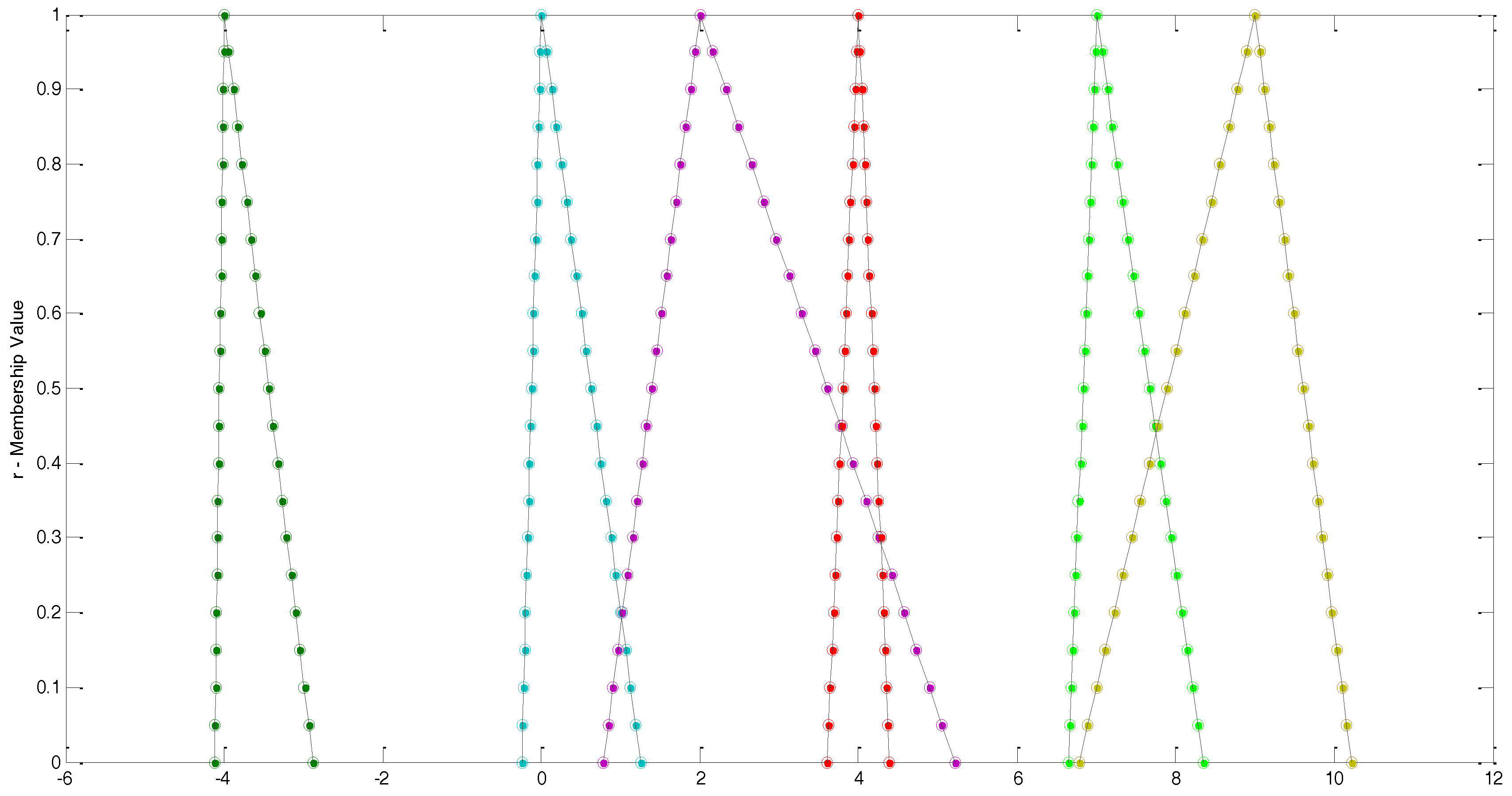
The exact and approximate solution using the Jacobi, Gauss–Seidel and the SOR iterative schemes are shown in Figure 1, Figure 2 and Figure 3 respectively. The Hausdoeff distance of solutions with $\epsilon ={10}^{-3}$ in the Jacobi method is 0.4091 × 10⁻³ in the Gauss–Seidel method is 0.4335 × 10⁻⁴ and in the SOR method with $\omega =1.3$ is 5.5611 × 10⁻⁴.

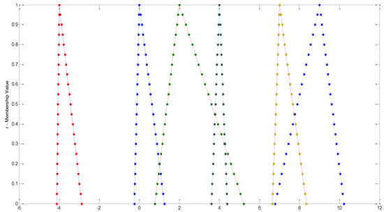
Figure 1. The Hausdorff distance of solutions with $\epsilon ={10}^{-3}$, in the Jacobi method is 0.4091 × 10⁻³.

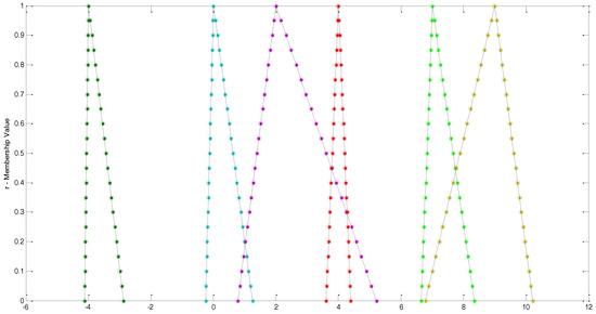
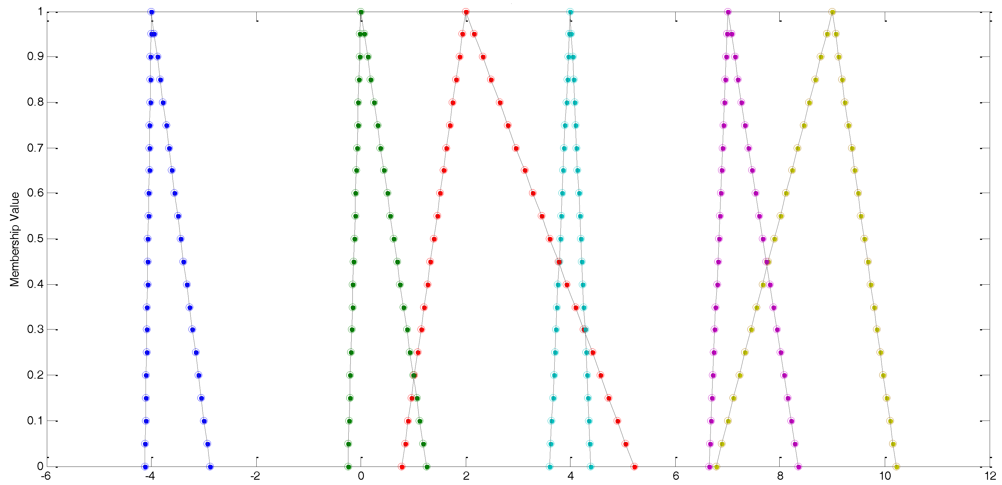
Figure 2. The Hausdorff distance of solutions with $\epsilon ={10}^{-3}$ in the Gauss–Seidel method is 0.4335 × 10⁻⁴.

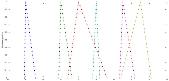
Figure 3. The Hausdorff distance of solutions with $\epsilon ={10}^{-3}$ in successive over-relaxation (SOR) method with $\omega =1.3$ is 5.5611 × 10⁻⁴.

5. Conclusions

In this article the Jacobi, Gauss–Seidel and SOR iterative methods have been used to solve the FSLEs where the coefficient matrix arrays are crisp numbers, the right-hand side column is an arbitrary fuzzy vector and the unknowns are fuzzy numbers. The numerical results have shown to be in a close agreement with the analytical ones. Moreover, Figure 1, Figure 2 and Figure 3 containing the Hausdorff distance of solutions show clearly that the SOR iterative method is more efficient in comparison with other iterative techniques.

References

- Zadeh, L.A. Fuzzy sets. Inf. Control 1965, 8, 338–353. [Google Scholar] [CrossRef]
- Friedman, M.; Ming, M.; Kandel, A. Fuzzy linear systems. Fuzzy Sets Syst. 1998, 96, 201–209. [Google Scholar] [CrossRef]
- Allahviraloo, T. Numerical methods for fuzzy system of linear equations. Appl. Math. Comput. 2004, 155, 493–502. [Google Scholar]
- Allahviraloo, T. Successive over relaxation iterative method for fuzzy system of linear equations. Appl. Math. Comput. 2005, 62, 189–196. [Google Scholar]
- Dehghan, M.; Hashemi, B. Iterative solution of fuzzy linear systems. Appl. Math. Comput. 2006, 175, 645–674. [Google Scholar] [CrossRef]
- Ezzati, R. Solving fuzzy linear systems. Soft Comput. 2011, 15, 193–197. [Google Scholar] [CrossRef]
- Muzzioli, S.; Reynaerts, H. Fuzzy linear systems of the form . Fuzzy Sets Syst. 2006, 157, 939–951. [Google Scholar]
- Abbasbandy, S.; Jafarian, A. Steepest descent method for system of fuzzy linear equations. Appl. Math. Comput. 2006, 175, 823–833. [Google Scholar] [CrossRef]
- Ineirat, L. Numerical Methods for Solving Fuzzy System of Linear Equations. Master’s Thesis, An-Najah National University, Nablus, Palestine, 2017. [Google Scholar]
- Asady, B.; Abbasbandy, S.; Alavi, M. Fuzzy general linear systems. Appl. Math. Comput. 2005, 169, 34–40. [Google Scholar] [CrossRef]
- Senthilkumar, P.; Rajendran, G. An algorithmic approach to solve fuzzy linear systems. J. Inf. Comput. Sci. 2011, 8, 503–510. [Google Scholar]
- Bede, B. Product type operations between fuzzy numbers and their applications in geology. Acta Polytech. Hung. 2006, 3, 123–139. [Google Scholar]
- Abbasbandy, S.; Alavi, M. A method for solving fuzzy linear systems. Iran. J. Fuzzy Syst. 2005, 2, 37–43. [Google Scholar]
- Amrahov, S.; Askerzade, I. Strong solutions of the fuzzy linear systems. CMES-Comput. Model. Eng. Sci. 2011, 76, 207–216. [Google Scholar]
© 2018 by the authors. Licensee MDPI, Basel, Switzerland. This article is an open access article distributed under the terms and conditions of the Creative Commons Attribution (CC BY) license (http://creativecommons.org/licenses/by/4.0/).