Article

Fractional Modeling for Quantitative Inversion of Soil-Available Phosphorus Content

1
College of Information Engineering, Qujing Normal University, Qujing 655011, China
2
College of Applied Arts and Science, Beijing Union University, Beijing 100083, China
*
Authors to whom correspondence should be addressed.
Mathematics 2018, 6(12), 330; https://doi.org/10.3390/math6120330
Submission received: 11 November 2018 / Revised: 3 December 2018 / Accepted: 3 December 2018 / Published: 14 December 2018

Abstract

:
The study of field spectra based on fractional-order differentials has rarely been reported, and traditional integer-order differentials only perform the derivative calculation for 1st-order or 2nd-order spectrum signals, ignoring the spectral transformation details between 0th-order to 1st-order and 1st-order to 2nd-order, resulting in the problem of low-prediction accuracy. In this paper, a spectral quantitative analysis model of soil-available phosphorus content based on a fractional-order differential is proposed. Firstly, a fractional-order differential was used to perform a derivative calculation of original spectral data from 0th-order to 2nd-order using 0.2-order intervals, to obtain 11 fractional-order spectrum data. Afterwards, seven bands with absolute correlation coefficient greater than 0.5 were selected as sensitive bands. Finally, a stepwise multiple linear regression algorithm was used to establish a spectral estimation model of soil-available phosphorus content under different orders, then the prediction effect of the model under different orders was compared and analyzed. Simulation results show that the best order for a soil-available phosphorus content regression model is a 0.6 fractional-order, the coefficient of determination ( R 2 ), root mean square error (RMSE), and ratio of performance to deviation (RPD) of the best model are 0.7888, 3.348878, and 2.001142, respectively. Since the RPD value is greater than 2, the optimal fractional model established in this study has good quantitative predictive ability for soil-available phosphorus content.

1. Introduction

Soil-available phosphorus refers to inorganic phosphorus or small molecular organic phosphorus that can be directly absorbed and utilized by plants [1,2,3]. Its content refers to the amount of phosphorus that can be absorbed by seasonal crops. It is an important indicator for evaluating the phosphorus supply capacity of soil phosphorus. Soil-phosphorus deficiency affects crop growth, while soil phosphorus in surplus for a long time increases the risk of soil phosphorus flowing into water bodies and creating potential ecological problems. The content of available phosphorus in soil varies with soil type, climate, fertilization level, irrigation, cultivation practices, and so on. Therefore, real-time detection of soil-available phosphorus content can provide a scientific reference for rational application of phosphate fertilizer and improvement of phosphate-fertilizer utilization. The traditional method for detecting soil-available phosphorus content is to adopt laboratory chemical reagents to measure, which has the disadvantage of being a cumbersome procedure, high-cost, and time-consuming [4,5,6]. Visible near-infrared spectroscopy has the characteristics of rapid, non-destructive, and low-cost detection [7,8,9]; it can analyze a large number of soil samples in a short time, and realize real-time online measurement of soil parameters.
A traditional integer-order differential method is widely used to process soil-spectral signals [10,11], but its description of the physical model is only an approximation, which largely ignores the authenticity of the system. Fractional calculus generalizes the order of traditional integer calculus to the field of fractions. Compared with traditional integer-order calculus, its greatest advantage lies in its memory and inheritance properties, which makes it more accurate and effective to describe certain physical phenomena by using fractional-order differential equations. It has been proved that fractional-order systems are more in line with natural laws and engineering physics phenomena. Fractional-order systems can better reflect the performance of dynamic systems and can more clearly describe the physical characteristics of the system. The composition of soil is very complex—it is mainly a mixture of minerals, organic matter, living organisms, water, and air. Fractional-order differential algorithms can be used to determine the inflection point of a soil spectral-reflectance curve and can perform baseline correction to eliminate background noise and atmospheric influence, distinguish overlapping spectra, and improve detection signal-to-noise ratio. It also can reduce the impact of soil type, sample size, and other factors; and excavate the spectral absorption characteristics.
In recent years, scholars have introduced fractional-order differentials into the field of spectral analysis, mainly focusing on the spectra of corn, wheat, and diesel in public collections; a few literature sources relate to soil spectra collected in an ideal indoor condition. For example, Kharintsev et al. [12] used a fractional derivative algorithm to separate the overlapping spectral features and extracted spectral characteristics, such as half-width and amplitude, showing that fractional differentials had certain feasibility in spectral analysis applications. Zheng et al. [13] utilized the Savitzky–Golay (SG) fractional derivative to preprocess near-infrared spectroscopy datasets for corn, wheat, and diesel; simulations showed that the preprocessing effect after fractional derivation was better than integer order. Zhang et al. [14] preprocessed the indoor spectrum of saline soil in Xinjiang by a fractional derivative algorithm; simulations showed that the effect of a fractional differential was significantly better than that of an integer-order differential. Wang et al. [15] studied the hyperspectral detection of chromium content by fractional differential algorithms and found that the 1.8-order differential model was the optimal model.
Some scholars, however, have applied the fractional-order differential method to study soil spectra under an indoor controllable light source with ideal conditions. The indoor soil spectrum does not take into account the influence of complex factors in the field and a prediction model established by the indoor spectrum is difficult to extend directly into the field. At present, there are relatively few studies on soil-available phosphorus and the study of field spectra based on fractional-order differentials has rarely been reported. Therefore, this paper took the desert soil in Xinjiang as the research object to collect the field spectral signals. We studied the application of the Grünwald–Letnikov fractional differential in field spectrum data preprocessing and feature extraction, and fully exploited the useful information in the spectrum for the prediction model of available phosphorus content to obtain effective sensitive bands. In addition, the dynamic law of spectrum data with fractional order changes was discussed and the optimal scheme of fractional spectral modeling sought. Moreover, the research of this paper has enriched the method of soil hyperspectral-data preprocessing, improved the accuracy of hyperspectral prediction models of available phosphorus content, and provided scientific support and application reference for local precision agriculture.

2. Materials and Methods
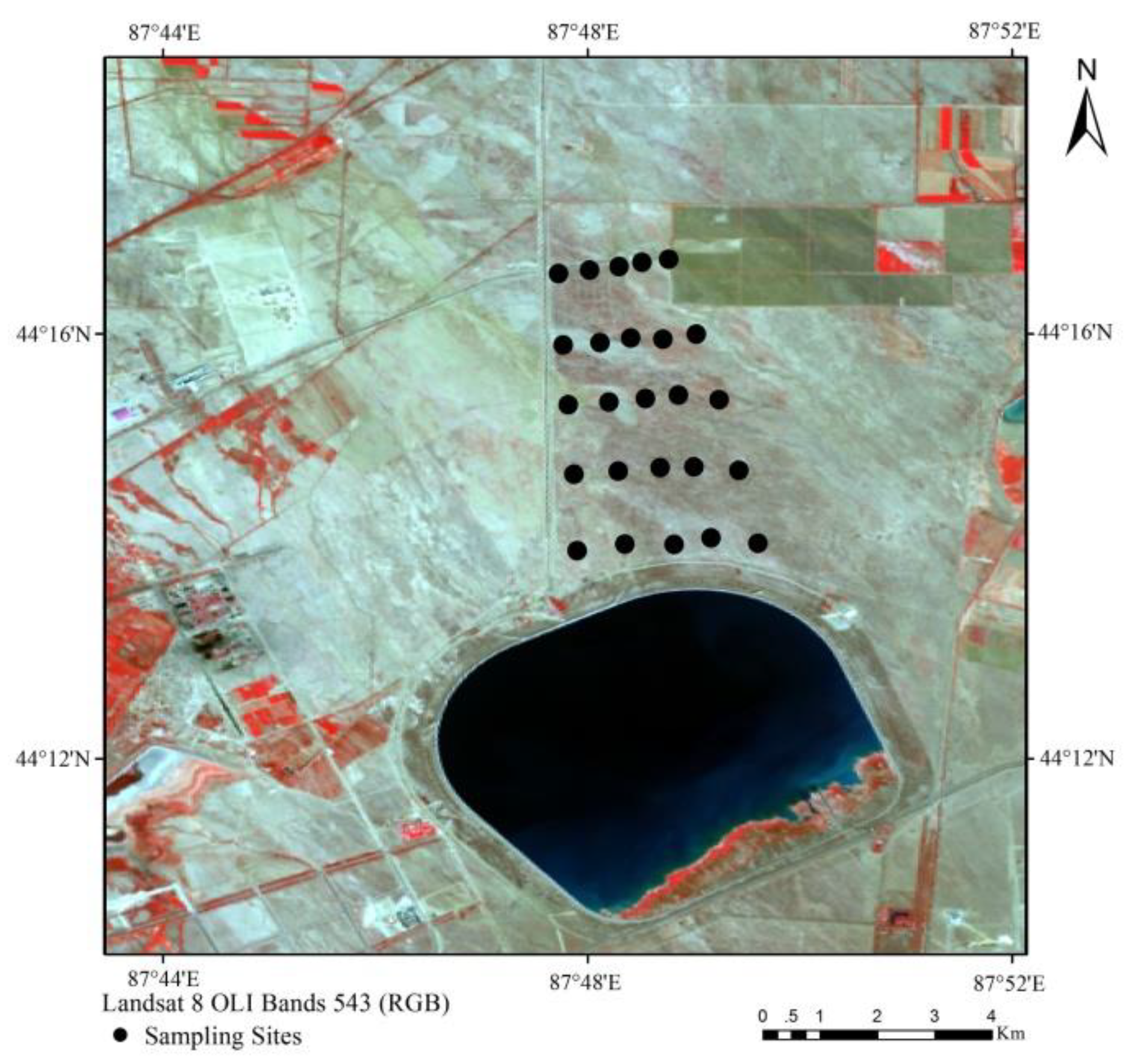
2.1. Research Area

The study area is located between the northern foot of the Tianshan Mountains and the southern margin of the Junggar Basin (87°44′–88°46′ E, 43°29′–45°45′ N). It belongs to the territory of Fukang in Xinjiang and has a pH value of 7.76–8.98. The characteristics of the Fukang terrain are low in the north and high in the south, with the landforms of mountainous in the south, plains in the middle, and deserts in the north. Fukang is a moderately temperate desert climate with plenty of light in the area. The average temperature in this region is 6.7 °C, the highest temperature is 39.7 °C, and the lowest temperature is −26.2 °C. The precipitation in this area is scarce, but the surface evaporation is very large.

2.2. Sampling Point Layout and Measurement of Available Phosphorus Content

In mid-May 2017, we arranged five sampling lines from south to north in the study area, with sampling line spacings of 600–800 m. Five sampling points on each sampling line were selected to represent the soil background in this area, the sampling distance was 300–500 m. A total of 25 sampling points was obtained and Global Positioning System (GPS) positioning was performed. The position distribution of the sampling points is shown in Figure 1.
Soil samples of 0–10 cm were collected from each sampling point, were numbered into bags, and brought back to the laboratory. All of the soil samples were air-dried naturally, had impurities removed, and were sieved through a 1 mm aperture. Then they were sent to the Xinjiang Institute of Ecology and the Geography of the Chinese Academy of Sciences to determine soil-available phosphorus content.

2.3. Field Spectral Data Acquisition

The ASD FieldSpec® 3Hi-Res (Malvern Panalytical Ltd, Malvern, UK) spectrometer was used to acquire field spectra on 9–23 May 2017. Its measured spectral range is 350–2500 nm, the sampling interval of the spectrum was 1.3 nm at 350–1000 nm, 2 nm at 1000–2500 nm, and the re-sampling interval was 1 nm. Since weather conditions affect the spectral measurement, in order to reduce the data error caused by weather conditions, the spectral measurement was selected to be carried out at 11:00–15:00 o’clock local time in sunny, cloudless, and windless weather. Before each spectral measurement, the spectrometer needed to be calibrated with a white board to remove dark current effects. Spectral probes were placed at a vertical distance of 15 cm above the surface of sampling points to represent the characteristics of this area. The ground surface was flat, with no cracks, and no weeds around. Spectral acquisition was performed in the same manner for each point, by selecting five position points close to the soil background value within a range of 1 m. Ten spectral curves were repeatedly measured at each sampling point, for a total of 50, and the mean value was taken as the actual measured spectrum value of the sampling point.
Before performing the subsequent data analysis, firstly, the SG smoothing method was used to smooth the spectrum, and then the spectral reflectances at 350 nm–400 nm in the ultraviolet bands and 2400 nm–2500 nm in the short-wavelength infrared bands were eliminated, because the signal-to-noise ratio of these bands was relatively low. Finally, the wavelength bands (1355–1410 nm, 1820–1942 nm) located in the moisture absorption zone were eliminated because these bands have a great influence on the accuracy of the spectral inversion of available phosphorus content.

2.4. Fractional Derivative

At present, the expressions of fractional differential mainly include Riemann–Liouville, Grünwald–Letnikov, and Caputo [16,17,18], and the most commonly used expressions are Grünwald–Letnikov (G–L) expressions. The G–L differential is defined by:
a D t v s ( t ) = lim h 0 s h v ( t ) = lim h 0 h v 0 r < C r v s ( t r h )
where the coefficient is:
C r v = ( ν ) ( ν + 1 ) ( ν + r 1 ) r ! .
According to the definition in Equation (1), suppose that the duration of signal s ( t ) is t [ a , t ] . Because we used the ASD Field Spec® 3Hi-Res spectrometer to collect field spectra, the re-sampling interval was 1 nm, and therefore, the signal duration for [ a , t ] was divided equally into equal intervals of h = 1 , then n can be defined as follows:
n = [ t a h ] h 1 = [ t a ] .
We can further deduce that the v-order fractional differential form expression of the signal s ( t ) is:
d ν s ( t ) d t ν s ( t ) + ( ν ) s ( t 1 ) + ( ν ) ( ν + 1 ) 2 s ( t 2 ) + ( ν ) ( ν + 1 ) ( ν + 2 ) 6 s ( t 3 ) + + Γ ( ν + 1 ) n ! Γ ( ν + n + 1 ) s ( t n ) .
From Equation (4), the difference coefficient of fractional differential can be described as follows:
a 0 = 1 , a 1 = ν , a 2 = ( ν ) ( ν + 1 ) 2 , a 3 = ( ν ) ( ν + 1 ) ( ν + 2 ) 6 , , a n = Γ ( ν + 1 ) n ! Γ ( ν + n + 1 )
where, v is an order, the 0th-order differential of function s ( t ) is s ( t ) itself which does not perform differential processing. For v = 1 and 2, respectively, Equation (4) agrees with the 1st and 2nd-order differential formulas when the differential window scale is ϖ = 1 .

2.5. Stepwise Multiple Linear Regression

Stepwise multiple linear regression (SMLR) is an optimization process based on a general multivariate regression analysis method [19,20]. The multiple linear regression model is a regression model composed of multiple independent variables that reveals the linear relationship between multiple independent variables and dependent variables.
Y is a dependent variable. X 1 , X 2 , , X m are m known independent variables and the number of samples is n . In the regression equations, the independent variable X i ( i = 1 , 2 , , k ) gives a significant effect to Y . For different fractional orders, we need to find which factors X i contribute to Y . Selection and rejection of independent variables for stepwise multiple regression analysis method is determined by the F statistic. The SMLR method is given as follows.
Step 1: Choose one variable x k 1 from m variables to establish a linear regression equation:
y = a 0 + a k 1 ( 1 ) x k 1 .
Step 2: Select the second of the remaining m 1 variables that has the most significant effect on y and establish a binary regression equation:
y = a 0 + a k 1 ( 1 ) x k 1 + a k 2 ( 2 ) x k 2 .
Check whether it is significant or not. If it is not, return to step one. If it is, continue to find the next variable.
Step 3: The regression equation is obtained.
y = a 0 + a k 1 ( 1 ) x k 1 + a k 2 ( 2 ) x k 2 + + a k k ( k - 1 ) x k k , k m .

2.6. Model Accuracy Verification Method

In order to evaluate comprehensively the accuracy of the SMLR quantitative estimation model, we selected three accuracy evaluation indicators [21]: root mean square error (RMSE), coefficient of determination ( R 2 ), and ratio of performance to deviation (RPD). R 2 was divided into the coefficient of determination for the calibration set ( R c 2 ) and the coefficient of determination for the verification set ( R p 2 ). The definition of RMSE, R 2 , and RPD can be described as follows:
RMSE = 1 n i = 1 n ( P i M i ) 2
R 2 = SSR SST
RPD = SD RMSE
where, n is the number of samples. Mi is the measured value of the i-th sample. Pi is the predicted value of the i-th sample. SSR represents the regression sum of squares. SST represents the sum of squares. SD is the standard deviation of validation sample. RMSE is the root mean square error of validation set.
When 0.66 ≤ R 2 ≤ 0.80, the model fitting effect is better [22]. When 0.81 ≤ R 2 ≤ 0.90, the model fitting result is very good. When R 2 ≥ 0.90, the model fitting effect is excellent. The closer the RMSE is to 0, the model has higher prediction accuracy and stronger the prediction ability.
When the RPD is greater than 2.5, it indicates that the model has strong predictive ability [23]. When the RPD is between 2.0 and 2.5, it indicates that the model has good quantitative prediction ability. When the RPD is between 1.8 and 2.0, it indicates that the model has quantitative predictive ability. When RPD is between 1.4 and 1.8, it indicates that the model has general quantitative prediction ability. When RPD is between 1.0 and 1.4, it indicates that the model only has the ability to distinguish between high and low values. When RPD is less than 1.0, it indicates that the model does not have predictive power.
For the calibration set, when R c 2 is larger, and RMSE is smaller, then the modeling accuracy of calibration set will be higher, and the model will be more stable. In addition, for the verification set, when R p 2 and RPD are larger, and RMSE is smaller, the prediction model has higher prediction accuracy.

3. Results and Discussion

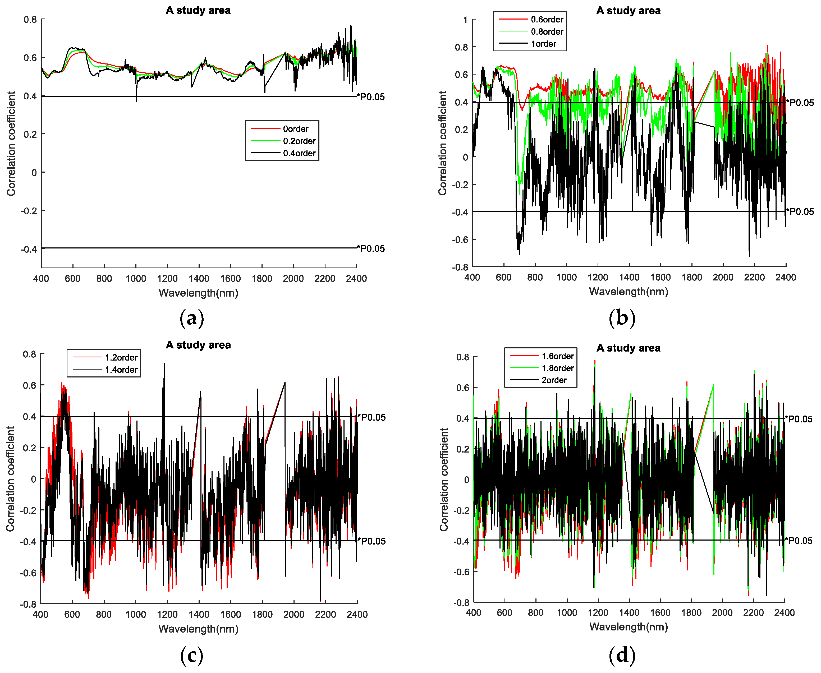
3.1. Correlation Coefficient

Original spectral reflectance was programmed in Matlab R2015a software (MathWorks, Natick, MA, USA), and the correlation coefficient between available phosphorus content and original spectral reflectance was calculated at 0.2-order intervals, with a total of 11 fractional differentials. The 0.05 significance test level in this area was *P0.05 = 0.396. Figure 2 shows the results of fractional processing of the original spectrum. The abscissa represents the wavelength and the ordinate represents the differential value of the spectral reflectance after fractional differential calculation. It can be seen from the simulation results that the original spectral reflectance has bands that passed 0.05 significance test from 0th-order, and the number of passed bands is large. Moreover, as the fractional order changes, more information in the original spectral data is mined, and its subtle changes are more obvious. Taking the differential values of 700 nm and 800 nm in Figure 2a as an example, we found that the subtle changes in the original spectral image were amplified and, by observing Figure 2b–d, some of the details were more pronounced. As the fractional order increased, sharper peaks appeared in the spectral curve.

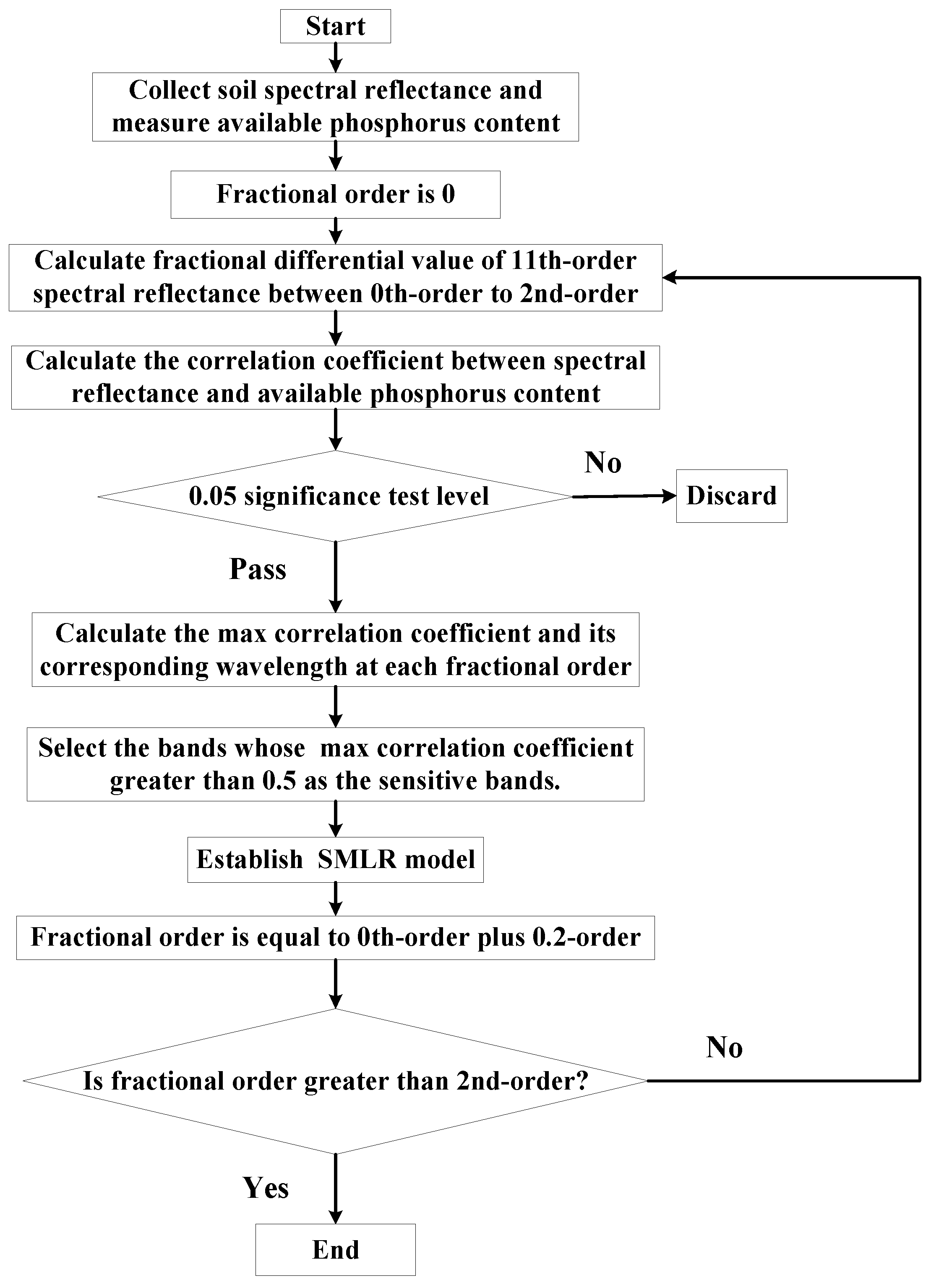
3.2. Modeling Process for Quantitative Analysis Model

The steps of the quantitative analysis model established in this paper are as follows:
Step 1:
Calculate the fractional differential value of 11 fractional differentials spectral reflectance between 0th-order and 2nd-order using Equation (4).
Step 2:
Calculate the correlation coefficient between spectral reflectance and available phosphorus content and perform a 0.05 significance test.
Step 3:
Statistically calculate the absolute value of the maximum correlation coefficient after the 11th-order fractional differential transformation and its corresponding wavelength.
Step 4:
Select the bands whose absolute value of maximum correlation coefficient with each fractional order is greater than 0.5 as the sensitive bands.
Step 5:
Establish the SMLR model.
Step 6:
All fractional spectral data and its corresponding sensitive bands are obtained by traversing 0th-order to 2nd-order at intervals of 0.2 step.
The flow chart of the quantitative analysis model for soil-available phosphorus content is shown in Figure 3.

3.3. Model Optimal Wavelength Selection

We have calculated the absolute value of the maximum correlation coefficient and its corresponding band information after the 11th-order fractional differential processing, which was shown in Table 1. The absolute value of the maximum correlation coefficient was 0.81085, the corresponding band was 2283 nm, and the order was 0.6. According to Table 1, the band with absolute value of maximum correlation coefficient greater than 0.5 is selected as the sensitive band, and there are seven bands in the study area. The selected bands are 1179, 2047, 2165, 2283, 2364, 2365, and 2393 nm, respectively.

3.4. Establishment Stepwise Multiple Linear Regression Model

Fifteen randomly selected samples from 25 soil samples were used to establish a model, and the other 10 samples were used as a validation set. Taking soil-available phosphorus content as a dependent variable, spectral reflectance was used as an independent variable for the sensitive bands 1179, 2047, 2165, 2283, 2364, 2365, and 2393 nm. The SMLR model was established to estimate available phosphorus content (Table 2).
In Table 2, Y is the soil-available phosphorus content, R 1179, R 2047, R 2165, R 2283, R 2364, R 2365 and R 2393 represent spectral reflectance values in the 1179, 2047, 2165, 2283, 2364, 2365, and 2393 nm wavelength bands. R 2 is 0.424 in 0th-order, R 2 is 0.591 in integer 1st-order, and R 2 is 0.644 in integer 2nd-order. After performing the fractional differential transformation by 0.4-order, 0.6-order, 0.8-order, 1.2-order, 1.4-order, 1.6-order and 1.8-order, R 2 has a certain degree of improvement. Among them, the 1.6-order improves the most and reaches 0.865. The RMSE is 5.13826 at 0th-order, 4.3324598 at 1st-order, and 4.040979 at 2nd-order. After fractional differential processing, RMSE decreased, and the lowest value of RMSE is 2.491789.

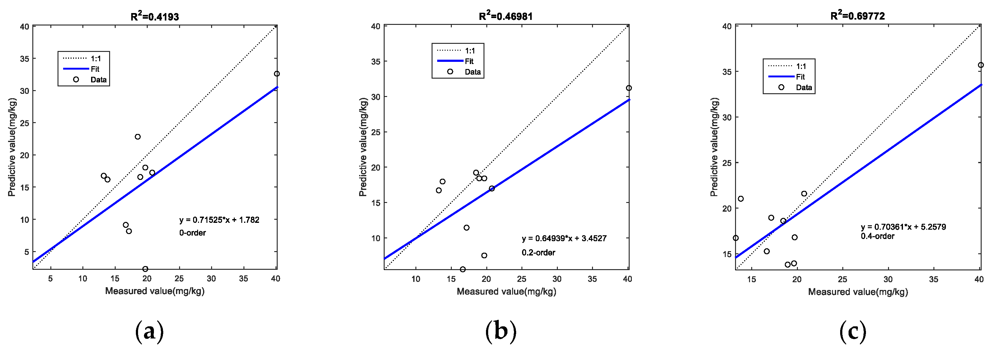
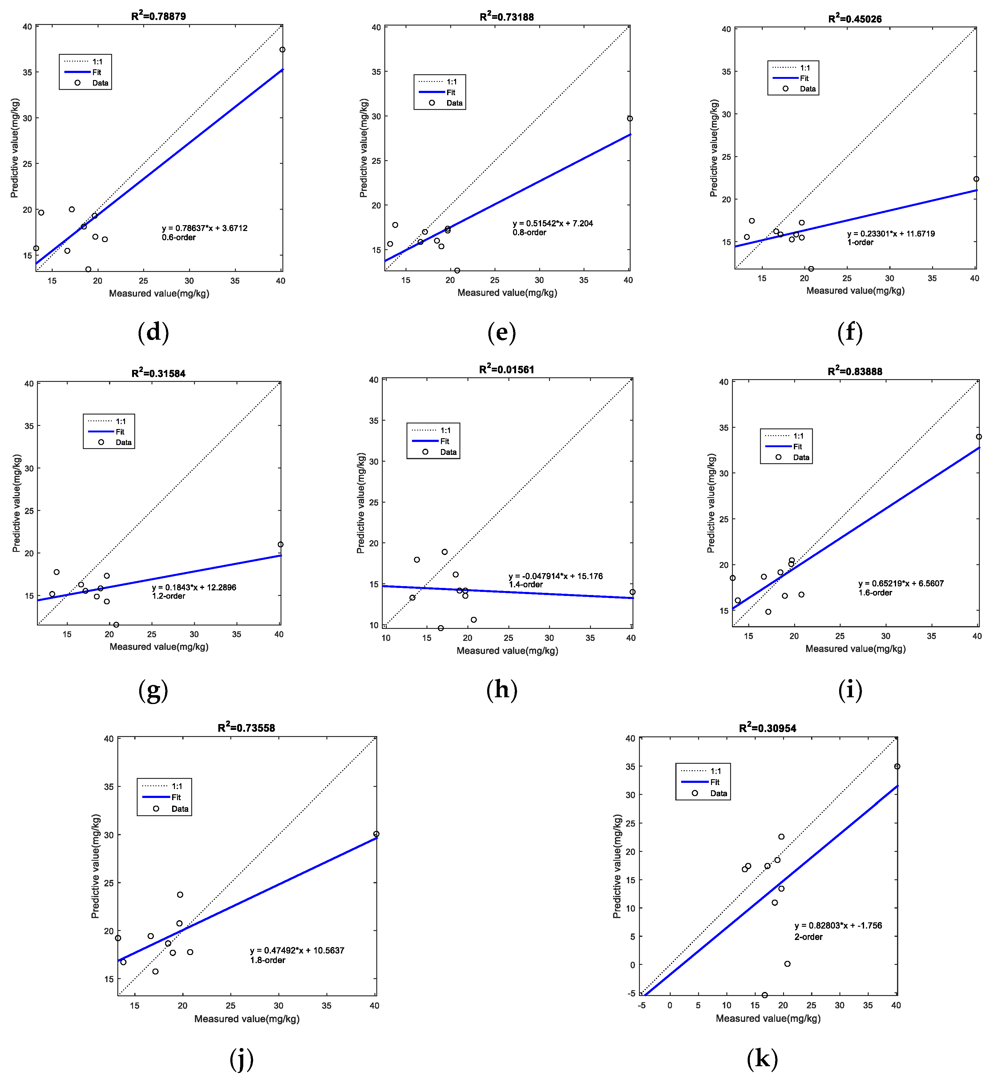
3.5. Predictive Model Accuracy Comparison

The root mean square error, R 2 and RPD were used as reference indexes for model evaluation (Table 3). Regression equations for 0.4-order, 0.6-order, 1.6-order and 1.8-order have relatively high R 2 and RPD values and relatively low RMSE values, indicating that these four differential orders have better prediction performance than other cases. The RPD value is greater than 2 at the 0.6-order, which indicates that the model has better prediction ability. The RPD values are between 1.4 and 2 in the range of 0.6, 1.6h, and 1.8-order, which indicates that the corresponding model predictability is general, and the available phosphorus content can be quantitatively estimated.

3.6. Selection Best Prediction Model

In order to obtain the best predictive model of available phosphorus content, 10 samples were used to verify the relationship between the measured and predicted values in Figure 4. For the 0.6-order, the verification set sample data points are all distributed along the 1:1 straight line, and the prediction correlation is better than for other orders. In general, based on the SMLR model of 0.6-order, the R 2 is higher, the RMSE is the smallest, and the RPD is the largest. Therefore, this model is the best prediction model for the available potassium content.

4. Conclusions

In this paper, the spectra of desert soils were collected in a field environment, and the spectral data were preprocessed using the Grünwald–Letnikov fractional differential. The seven sensitive bands were identified by the correlation analysis method. The bands estimated soil-available phosphorus content are 1179, 2047, 2165, 2283, 2364, 2365, and 2393 nm. According to varied fractional derivatives, we obtained different regression equations where different sensitive bands were independent variables. The fractional derivative played an important role to in finding major independents and the SMLR model and gave the regressive relationships. An optimal fractional prediction model for soil-available phosphorus content was finally provided. The method proved to be efficient in this study. In the future, we will consider neural network, machine learning, and similar algorithms to improve the prediction accuracy and other applications in the spectrum analysis field.

Author Contributions

C.F. designed the research and performed all the modeling. A.T. and H.X. collected the experiment data. A.T. was involved in drafting and revising the manuscript.

Funding

The authors would like to thank the financial support of the National Natural Science Foundation of China (41671198), the Yunnan Province Science and Technology Department and the Education Department Project (2017FH001-067, 2017FH001-117), China.

Conflicts of Interest

The authors declare no conflict of interest.

References

  1. Shao, Y.; He, Y. Nitrogen, phosphorus, and potassium prediction in soils, using infrared spectroscopy. Soil Res. 2011, 49, 166–172. [Google Scholar] [CrossRef]
  2. Mouazen, A.M.; Kuang, B.; de Baerdemaeker, J.; Ramon, H. Comparison among principal component, partial least squares and back propagation neural network analyses for accuracy of measurement of selected soil properties with visible and near infrared spectroscopy. Geoderma 2010, 158, 23–31. [Google Scholar] [CrossRef]
  3. Zhang, W.; Zeng, G.; Chen, X.; Lin, W. Spatial-temporal pattern and source of soil available phosphorus in Minjiang River estuarine wetland. Chin. J. Ecol. 2015, 34, 168–174. [Google Scholar]
  4. Sarathjith, M.C.; Das, B.S.; Wani, S.P.; Sahrawat, K.L.; Gupta, A. Comparison of Data Mining Approaches for Estimating Soil Nutrient Contents Using Diffuse Reflectance Spectroscopy. Curr. Sci. 2016, 110, 1031. [Google Scholar] [CrossRef]
  5. Balabin, R.M.; Safieva, R.Z.; Lomakina, E.I. Wavelet neural network (WNN) approach for calibration model building based on gasoline near infrared (NIR) spectra. Chemometr. Intell. Lab. Syst. 2008, 93, 58–62. [Google Scholar] [CrossRef]
  6. Mouaze, A.M.; Maleki, M.R.; Baerdemaeker, J.D.; Ramon, H. On-line measurement of some selected soil properties using a VIS–NIR sensor. Soil Tillage Res. 2007, 93, 13–27. [Google Scholar] [CrossRef]
  7. Paz-Kagan, T.; Zaady, E.; Salbach, C.; Schmidt, A.; Lausch, A.; Zacharias, S.; Notesco, G.; Ben-Dor, E.; Karnieli, A. Mapping the Spectral Soil Quality Index (SSQI) Using Airborne Imaging Spectroscopy. Remote Sens. 2015, 7, 15748–15781. [Google Scholar] [CrossRef] [Green Version]
  8. Bo, S.; Raphaela, V.R.; Abdulmounem, M.; Johanna, W. Visible and near infrared spectroscopy in soil science. Adv. Agron. 2010, 107, 163–215. [Google Scholar]
  9. Gholizadeh, A.; Boruvka, L.; Saberioon, M.; Němeček, K. Comparing different data preprocessing methods for monitoring soil heavy metals based on soil spectral features. Soil Water Res. 2015, 10, 218–227. [Google Scholar] [CrossRef]
  10. Rajeev, S.; Madhurama, S.; Yadav, R.K.; Bundela, D.S.; Manjeet, S.; Chattaraj, S.; Singh, S.K. Visible-Near Infrared Reflectance Spectroscopy for Rapid Characterization of Salt-Affected Soil in the Indo-Gangetic Plains of Haryana, India. J. Indian Soc. Remote Sens. 2016, 45, 307–315. [Google Scholar]
  11. Jia, S.; Yang, X.; Li, G.; Zhang, J. Quantitatively Determination of Available Phosphorus in Soil by Near Infrared Spectroscopy Combining with Recurisive Partial Least Squares. Spectrosc. Spectr. Anal. 2015, 35, 2516–2520. [Google Scholar]
  12. Kharintsev, S.S.; Salakhov, M.K. Peak Parameters Determination Using Fractional Derivative Spectrometry; Astronomical Observatory of Belgrade: Beograd, Serbia, 2003; pp. 211–214. [Google Scholar]
  13. Zheng, K.-Y.; Zhang, X.; Tong, P.-J.; Yao, Y.; Du, Y.-P. Pretreating near infrared spectra with fractional order Savitzky–Golay differentiation (FOSGD). Chin. Chem. Lett. 2015, 26, 293–296. [Google Scholar] [CrossRef]
  14. Zhang, D.; Tashpolat, T.; Ding, J.; Wang, J. Quantitative Estimating Salt Content of Saline Soil Using Laboratory Hyperspectral Data Treated by Fractional Derivative. J. Spectrosc. 2016, 2016. [Google Scholar] [CrossRef]
  15. Wang, J.; Tashpolat, T.; Zhang, D. Spectral Detection of Chromium Content in Desert Soil Based on Fractional Differential. Trans. Chin. Soc. Agric. Mach. 2017, 152–158. [Google Scholar] [CrossRef]
  16. Angstmann, C.N.; Henry, B.I.; Mcgann, A.V. Discretization of Fractional Differential Equations by a Piecewise Constant Approximation. Math. Model. Nat. Phenom. 2016, 12, 23–26. [Google Scholar] [CrossRef]
  17. Almusalhi, F.; Alsalti, N.; Kerbal, S. Inverse Problems of a Fractional Differential Equation with Bessel Operator. Math. Model. Nat. Phenom. 2017, 12, 105–113. [Google Scholar] [CrossRef] [Green Version]
  18. Galeone, L.; Garrappa, R. Explicit Methods for Fractional Differential Equations and Their Stability Properties. J. Comput. Appl. Math. 2009, 228, 548–560. [Google Scholar] [CrossRef]
  19. Latt, Z.Z.; Wittenberg, H. Improving Flood Forecasting in a Developing Country: A Comparative Study of Stepwise Multiple Linear Regression and Artificial Neural Network. Water Resour. Manag. 2014, 28, 2109–2128. [Google Scholar] [CrossRef]
  20. Zhong, P.; Zhang, P.; Wang, R. Dynamic Learning of SMLR for Feature Selection and Classification of Hyperspectral Data. IEEE Geosci. Remote Sens. Lett. 2008, 5, 280–284. [Google Scholar] [CrossRef]
  21. Qiao, X.-X.; Wang, C.; Feng, M.-C.; Yang, W.-D.; Ding, G.-W.; Sun, H.; Liang, Z.-Y.; Shi, C.C. Hyperspectral estimation of soil organic matter based on different spectral preprocessing techniques. Spectrosc. Lett. 2017, 50, 156–163. [Google Scholar] [CrossRef]
  22. Wang, H.; Zhang, Z.; Arnon, K.; Chen, J.; Han, W. Hyperspectal estimation of desert soil organic matter content based on gray correlation-ridge regressing model. Trans. Chin. Soc. Agric. Eng. 2018, 34, 124–131. [Google Scholar]
  23. Zhang, Q.; Zhang, H.; Zhang, H.; Wang, X.; Liu, W. Hybrid inversion model of heavy metals with hyperspectral reflectance in cultivated soils of main grain producing areas. Trans. Chin. Soc. Agric. Mach. 2017, 48, 148–155. [Google Scholar]
Figure 1. Distribution of sampling points.
Mathematics 06 00330 g001
Figure 2. Correlation coefficients between available phosphorus content and soil spectrum with orders: (a) 0–0.4; (b) 0.6–1; (c) 1.2–1.4; (d) 1.6–2.
Mathematics 06 00330 g002
Figure 3. Flow chart of the quantitative analysis model.
Mathematics 06 00330 g003
Figure 4. Measured values versus predicted values for verification set: (a) 0th-order; (b) 0.2-order; (c) 0.4-order; (d) 0.6-order; (e) 0.8-order; (f) 1st-order; (g) 1.2-order; (h) 1.4-order; (i) 1.6-order; (j) 1.8-order; (k) 2nd-order.
Mathematics 06 00330 g004aMathematics 06 00330 g004b
Table 1. Absolute value of maximum correlation coefficient of the 11th-order differential and its corresponding band.
Fractional OrderCorrelation CoefficientBand
0.00.670762393
0.20.702522365
0.40.766982364
0.60.810852283
0.80.762302047
1.00.728282165
1.20.785612165
1.40.782762165
1.60.778281179
1.80.748031179
2.00.761872283
Table 2. Stepwise multiple linear regression (SMLR) model for soil-available phosphorus content.
Fractional Order R 2 RMSERegression Equation
0.00.4245.138126Y = −7.877 + 73.319 × R2393
0.20.4874.849662Y = 11.929 + 713.184 × R2365 − 646.632 × R2165
0.40.7613.309459Y = 12.091 + 1852.579 × R2364 − 1605.108 × R1179
0.60.7503.382826Y = 17.181 − 7257.243 × R2283 − 13134.640 × R2047 − 57458.127 × R1179
0.80.7443.427327Y = −3.514 + 9907.544 × R2047 − 4796.115 × R2165
1.00.5914.3324598Y = 12.962 − 11610.572 × R2165
1.20.7183.595593Y = 13.174 − 11574.405 × R2165
1.40.8092.961901Y = 19.099 − 7691.730 × R2165 + 80915.009 × R1179
1.60.8652.491789Y = 16.654 − 8411.379 × R2165 + 75168.550 × R1179 − 1140.389 × R2365
1.80.8242.865772Y = 17.240 − 7227.992 × R2283 − 13268.074 × R2047 − 63874.358 × R1179 + 1008.311 × R2365
2.00.6444.040979Y = 19.020 − 8316.207 × R2283
RMSE: root mean square error.
Table 3. Accuracy evaluation for the SMLR prediction model.
Fractional Order R 2 RMSERPD
0.00.41937.4627481.120282
0.20.46986.5709871.091302
0.40.69773.9974341.594921
0.60.78883.3488782.001142
0.80.73184.7916800.951661
1.00.45036.8102290.385937
1.20.31587.3030340.339882
1.40.01569.7846260.296595
1.60.83893.2507591.657943
1.80.73564.2913051.476663
2.00.309510.3492631.088459

