An Efficient Family of Optimal Eighth-Order Multiple Root Finders

Abstract

Finding a repeated zero for a nonlinear equation $f\left(x\right)=0$, $f:I\subseteq R\to R$ has always been of much interest and attention due to its wide applications in many fields of science and engineering. Modified Newton’s method is usually applied to solve this kind of problems. Keeping in view that very few optimal higher-order convergent methods exist for multiple roots, we present a new family of optimal eighth-order convergent iterative methods for multiple roots with known multiplicity involving a multivariate weight function. The numerical performance of the proposed methods is analyzed extensively along with the basins of attractions. Real life models from life science, engineering, and physics are considered for the sake of comparison. The numerical experiments and dynamical analysis show that our proposed methods are efficient for determining multiple roots of nonlinear equations.

1. Introduction

It is well-known that Newton’s method converges linearly for non-simple roots of a nonlinear equation. For obtaining multiple roots of a univariate nonlinear equation with a quadratic order of convergence, Schröder [1] modified Newton’s method with prior knowledge of the multiplicity $m\ge 1$ of the root as follows:

$$x_{n+1}=x_n-m\frac{f\left(x_n\right)}{f^{\prime }\left(x_n\right)}.$$

(1)

Scheme (1) can determine the desired multiple root with quadratic convergence and is optimal in the sense of Kung-Traub’s conjecture [2] that any multipoint method without memory can reach its convergence order of at most $2^{p-1}$ for p functional evaluations.

In the last few decades, many researchers have worked to develop iterative methods for finding multiple roots with greater efficiency and higher order of convergence. Among them, Li et al. [3] in 2009, Sharma and Sharma [4] and Li et al. [5] in 2010, Zhou et al. [6] in 2011, Sharifi et al. [7] in 2012, Soleymani et al. [8], Soleymani and Babajee [9], Liu and Zhou [10] and Zhou et al. [11] in 2013, Thukral [12] in 2014, Behl et al. [13] and Hueso et al. [14] in 2015, and Behl et al. [15] in 2016 presented optimal fourth-order methods for multiple zeros. Additionally, Li et al. [5] (among other optimal methods) and Neta [16] presented non-optimal fourth-order iterative methods. In recent years, efforts have been made to obtain an optimal scheme with a convergence order greater than four for multiple zeros with multiplicity $m\ge 1$ of univariate function. Some of them only succeeded in developing iterative schemes of a maximum of sixth-order convergence, in the case of multiple zeros; for example, see [17,18]. However, there are only few multipoint iterative schemes with optimal eighth-order convergence for multiple zeros which have been proposed very recently.

Behl et al. [19] proposed a family of optimal eighth-order iterative methods for multiple roots involving univariate and bivariate weight functions given as:

$$\begin{array}{cc}\hfill y_n& =x_n-m\frac{f\left(x_n\right)}{f^{\prime }\left(x_n\right)},m\ge 1,\hfill \\ \hfill z_n& =y_n-u_{n}Q\left(h_n\right)\frac{f\left(x_n\right)}{f^{\prime }\left(x_n\right)},\hfill \\ \hfill x_{n+1}& =z_n-u_n{t}_{n}G(h_n,t_n)\frac{f\left(x_n\right)}{f^{\prime }\left(x_n\right)},\hfill \end{array}$$

(2)

where weight functions $Q:\mathbb{C}\to \mathbb{C}$ and $G:{\mathbb{C}}^2\to \mathbb{C}$ are analytical in neighborhoods of $\left(0\right)$ and $(0,0),$ respectively, with $u_n={\left(\frac{f\left(y_n\right)}{f\left(x_n\right)}\right)}^{\frac{1}{m}},$ $h_n=\frac{u_n}{a_1+a_2{u}_n}$ and $t_n={\left(\frac{f\left(z_n\right)}{f\left(y_n\right)}\right)}^{\frac{1}{m}},$ being $a_1$ and $a_2$ complex nonzero free parameters.

A second optimal eighth-order scheme involving parameters has been proposed by Zafar et al. [20], which is given as follows:

$$\begin{array}{cc}\hfill y_n& =x_n-m\frac{f\left(x_n\right)}{f^{\prime }\left(x_n\right)},m\ge 1,\hfill \\ \hfill z_n& =y_n-m{u}_{n}H\left(u_n\right)\frac{f\left(x_n\right)}{f^{\prime }\left(x_n\right)},\hfill \\ \hfill x_{n+1}& =z_n-u_n{t}_n(B_1+B_2{u}_n)P\left(t_n\right)G\left(w_n\right)\frac{f\left(x_n\right)}{f^{\prime }\left(x_n\right)},\hfill \end{array}$$

(3)

where $B_1$,$B_2\in \mathbb{R}$ are free parameters and the weight functions $H:\mathbb{C}\to \mathbb{C},$ $P:\mathbb{C}\to \mathbb{C}$ and $G:\mathbb{C}\to \mathbb{C}$ are analytic in the neighborhood of 0 with $u_n={\left(\frac{f\left(y_n\right)}{f\left(x_n\right)}\right)}^{\frac{1}{m}},$ $t_n={\left(\frac{f\left(z_n\right)}{f\left(y_n\right)}\right)}^{\frac{1}{m}}$ and $w_n={\left(\frac{f\left(z_n\right)}{f\left(x_n\right)}\right)}^{\frac{1}{m}}.$

Recently, Geum et al. [21] presented another optimal eighth-order method for multiple roots:

$$\begin{array}{cc}\hfill y_n& =x_n-m\frac{f\left(x_n\right)}{f^{\prime }\left(x_n\right)},n\ge 0\hfill \\ \hfill w_n& =x_n-m{L}_f\left(s\right)\frac{f\left(x_n\right)}{f^{\prime }\left(x_n\right)},\hfill \\ \hfill x_{n+1}& =x_n-m\left[L_f\left(s\right)+K_f\left(s,u\right)\right]\frac{f\left(x_n\right)}{f^{\prime }\left(x_n\right)},\hfill \end{array}$$

(4)

where $L_f:\mathbb{C}\to \mathbb{C}$ is analytic in the neighborhood of 0 and $K_f:{\mathbb{C}}^2\to \mathbb{C}$ is holomorphic in the neighborhood of $\left(0,0\right)$ with $s={\left(\frac{f\left(y_n\right)}{f\left(x_n\right)}\right)}^{\frac{1}{m}},$ $u={\left(\frac{f\left(w_n\right)}{f\left(y_n\right)}\right)}^{\frac{1}{m}}.$

Behl et al. [22] also developed another optimal eighth-order method involving free parameters and a univariate weight function as follows:

$$\begin{array}{cc}\hfill y_n& =x_n-m\frac{f\left(x_n\right)}{f^{\prime }\left(x_n\right)},\hfill \\ \hfill z_n& =y_n-mu\frac{f\left(x_n\right)}{f^{\prime }\left(x_n\right)}\frac{1+\beta u}{1+(\beta -2)u},\beta \in \mathbb{R}\hfill \\ \hfill x_{n+1}& =z_n-uv\frac{f\left(x_n\right)}{f^{\prime }\left(x_n\right)}\left({\alpha }_1+(1+{\alpha }_{2}v)P_f\left(u\right)\right),\hfill \end{array}$$

(5)

where ${\alpha }_1,{\alpha }_2\in \mathbb{R}$ are two free disposable parameters and the weight function $P_f:\mathbb{C}\to \mathbb{C}$ is an analytic function in a neighborhood of 0 with $u={\left(\frac{f\left(y_n\right)}{f\left(x_n\right)}\right)}^{\frac{1}{m}},v={\left(\frac{f\left(z_n\right)}{f\left(y_n\right)}\right)}^{\frac{1}{m}}.$

Most recently, Behl at al. [23] presented an optimal eighth-order method involving univariate weight functions given as:

$$\begin{array}{cc}\hfill y_n& =x_n-m\frac{f\left(x_n\right)}{f^{\prime }\left(x_n\right)},m\ge 1,\hfill \\ \hfill z_n& =y_n-m{u}_n{G}_f\left(u_n\right)\frac{f\left(x_n\right)}{f^{\prime }\left(x_n\right)},\hfill \\ \hfill x_{n+1}& =z_n+\frac{u_n{w}_n}{1-w_n}\frac{f\left(x_n\right)}{f^{\prime }\left(x_n\right)}\left(H_f\left(u_n\right)+K_f\left(v_n\right)\right),\hfill \end{array}$$

(6)

where $B_1$, $B_2\in \mathbb{R}$ are free parameters and the weight functions $G_f,H_f,K_f:\mathbb{C}\to \mathbb{C}$ are analytic in the neighborhood of 0 with $u_n={\left(\frac{f\left(y_n\right)}{f\left(x_n\right)}\right)}^{\frac{1}{m}},$ $v_n={\left(\frac{f\left(z_n\right)}{f\left(x_n\right)}\right)}^{\frac{1}{m}}$ and $w_n={\left(\frac{f\left(z_n\right)}{f\left(y_n\right)}\right)}^{\frac{1}{m}}.$

Motivated by the research going on in this direction and with a need to give more stable optimal higher-order methods, we propose a new family of optimal eighth-order iterative methods for finding simple as well as multiple zeros of a univariate nonlinear function with multiplicity $m\ge 1$. The derivation of the proposed class is based on a univariate and trivariate weight function approach. In addition, our proposed methods not only give the faster convergence but also have smaller residual error. We have demonstrated the efficiency and robustness of the proposed methods by performing several applied science problems for numerical tests and observed that our methods have better numerical results than those obtained by the existing methods. Further, the dynamical performance of these methods on the above mentioned problems supports the theoretical aspects, showing a good behavior in terms of dependence on initial estimations.

The rest of the paper is organized as follows: Section 2 provides the construction of the new family of iterative methods and the analysis of convergence to prove the eighth order of convergence. In Section 3, some special cases of the new family are defined. In Section 4, the numerical performance and comparison of some special cases of the new family with the existing ones are given. The numerical comparisons is carried out using the nonlinear equations that appear in the modeling of the predator–prey model, beam designing model, electric circuit modeling, and eigenvalue problem. Additionally, some dynamical planes are provided to compare their stability with that of known methods. Finally, some conclusions are stated in Section 5.

2. Construction of the Family

This section is devoted to the main contribution of this study, the design and convergence analysis of the proposed scheme. We consider the following optimal eighth-order class for finding multiple zeros with multiplicity $m\ge 1$:

$$\begin{array}{cc}\hfill y_n& =x_n-m\frac{f\left(x_n\right)}{f^{\prime }\left(x_n\right)},n\ge 0,\hfill \\ \hfill z_n& =y_n-m{u}_{n}G\left(u_n\right)\frac{f\left(x_n\right)}{f^{\prime }\left(x_n\right)},\hfill \\ \hfill x_{n+1}& =z_n-m{u}_{n}H(u_n,t_n,w_n)\frac{f\left(x_n\right)}{f^{\prime }\left(x_n\right)},\hfill \end{array}$$

(7)

where $G:\mathbb{C}\to \mathbb{C}$ and $H:{\mathbb{C}}^3\to \mathbb{C}$ are analytical functions in a neighborhood of $\left(0\right)$ and $(0,0,0),$ respectively being $u_n={\left(\frac{f\left(y_n\right)}{f\left(x_n\right)}\right)}^{\frac{1}{m}},$ $t_n={\left(\frac{f\left(z_n\right)}{f\left(y_n\right)}\right)}^{\frac{1}{m}}$ and $w_n={\left(\frac{f\left(z_n\right)}{f\left(x_n\right)}\right)}^{\frac{1}{m}}$.

In the next result, we demonstrate that the order of convergence of the proposed family reaches optimal order eight.

Theorem 1.

Let us consider $x=\xi$ (say) is a zero with multiplicity $m\ge 1$ of the involved function f. In addition, we assume that $f:\mathbb{C}\to \mathbb{C}$ is an analytical function in the region enclosing the multiple zero ξ. The proposed class defined by Equation (7) has an optimal eighth order of convergence, when the following conditions are satisfied:

$$\begin{array}{cc}\hfill G\left(0\right)& =1,G_1=G^{\prime }\left(0\right)=2,G_2=G^{″}\left(0\right)=4-\frac{G_3}{6},G_3=G^{‴}\left(0\right)\hfill \\ \hfill H_{000}& =0,H_{100}=0,H_{010}=1,H_{101}=3-\frac{G_3}{12},H_{110}=2-H_{001},\hfill \\ \hfill H_{011}& =4,H_{020}=1,\left|G_3\right|<\infty ,\left|H_{001}\right|<\infty ,\hfill \end{array}$$

(8)

where $H_{ijk}=\frac{1}{i!j!k!}\frac{{\partial }^{i+j+k}}{\partial u_n^j\partial t_n^j\partial w_n^k}H(u_n,t_n,w_n)|{}_{(u_n=0,t_n=0,w_n=0)}$ for $0\le i,k\le 1,0\le j\le 2$.

Proof. 

Let us assume that $e_n=x_n-\xi$ is the error at nth step. By expanding $f\left(x_n\right)$ and $f^{\prime }\left(x_n\right)$ about $x=\xi$ using Taylor series expansion, we have:

$$f\left(x_n\right)=\frac{f^{\left(m\right)}\left(\xi \right)}{m!}{e}_n^m\left(1+c_1{e}_n+c_2{e}_n^2+c_3{e}_n^3+c_4{e}_n^4+c_5{e}_n^5+c_6{e}_n^6+c_7{e}_n^7+c_8{e}_n^8+O\left(e_n^9\right)\right)$$

(9)

and:

$$\begin{array}{ll}{f}^{\prime }\left(x_n\right)& =\frac{f^{\left(m\right)}\left(\xi \right)}{m!}{e}_n^{m-1}\left(m+c_1(m+1)e_n+c_2(m+2)e_n^2+c_3(m+3)e_n^3+c_4(m+4)e_n^4+c_5(m+5)e_n^5\right.\\ & \left.+c_6(m+6)e_n^6+c_7(m+7)e_n^7+c_8(m+8)e_n^8+O\left(e_n^9\right)\right),\end{array}$$

(10)

respectively, where $c_k={\displaystyle \frac{m!}{(m+k)!}}{\displaystyle \frac{f^{(m+k)}\left(\xi \right)}{f^{\left(m\right)}\left(\xi \right)}},k=1,2,3,\cdots 8$.

By inserting the above Equations (9) and (10), in the first substep of Equation (7), we obtain:

$$y_n-\xi =\frac{c_1{e}_n^2}{m}+\frac{\left(2m{c}_2-(m+1)c_1^2\right)e_n^3}{m^2}+\sum _{k=0}^4{A}_k{e}_n^{k+4}+O\left(e_n^9\right),$$

(11)

where $A_k=A_k(m,c_1,c_2,\dots ,c_8)$ are given in terms of $m,c_1,c_2,c_3,\dots ,c_8$ with two explicitly written coefficients $A_0=\frac{1}{m^3}\left\{3c_3{m}^2+c_1^3{(m+1)}^2-c_1{c}_{2}m(3m+4)\right\}$ and $A_1=-\frac{1}{m^4}\left\{c_1^4{(m+1)}^3-2c_2{c}_1^{2}m(2m^2+5m+3)+2c_3{c}_1{m}^2(2m+3)+2m^2\left(c_2^2(m+2)-2c_{4}m\right)\right\},$ etc.

With the help of Taylor series expansion and Equation (11), we get:

$$f\left(y_n\right)=f^{\left(m\right)}\left(\xi \right)e_n^{2m}\left[\frac{{\left(\frac{c_1}{m}\right)}^m}{m!}+\frac{\left(2m{c}_2-(m+1)c_1^2\right){\left(\frac{c_1}{m}\right)}^m{e}_n}{m!c_1}+\sum _{k=0}^6{\overline{A}}_k{e}_n^{k+2}+O\left(e_n^9\right)\right].$$

(12)

Using Equations (9) and (12), we have:

$$u_n={\left(\frac{f\left(y_n\right)}{f\left(x_n\right)}\right)}^{\frac{1}{m}}=\frac{c_1{e}_n}{m}+\frac{\left(2m{c}_2-(m+2)c_1^2\right)e_n^2}{m^2}+{\tau }_1{e}_n^3+{\tau }_2{e}_n^4+{\tau }_3{e}_n^5+O\left(e_n^6\right),$$

(13)

where ${\tau }_1=\frac{1}{2m^3}\left[c_1^3(2m^2+7m+7)+6c_3{m}^2-2c_1{c}_{2}m(3m+7)\right],$ ${\tau }_2=-\frac{1}{6m^4}\left[c_1^4(6m^3+29m^2+51m+34)-6c_2{c}_1^{2}m(4m^2+16m+17)+12c_1{c}_3{m}^2(2m+5)+12m^2(c_2^2(m+3)-2c_{4}m)\right]$ and ${\tau }_3=\frac{1}{24m^5}\left[-24m^3\left(c_2{c}_3(5m+17)-5c_{5}m\right)+12c_3{c}_1^2{m}^2(10m^2+43m+49)+12c_1{m}^2\left\{c_2^2(10m^2+47m+53)-2c_{4}m(5m+13)\right\}-4c_2{c}_1^{3}m(30m^3+163m^2+306m+209)+c_1^5(24m^4+146m^3+355m^2+418m+209)\right]$.

It is clear from Equation (13) that $u_n$ is of order one. Therefore, we can expand the weight function $G\left(u_n\right)$ in the neighborhood of origin by Taylor series expansion up to third-order terms for eighth-order convergence as follows:

$$G\left(u_n\right)\approx G\left(0\right)+u_n{G}^{\prime }\left(0\right)+\frac{u_n^2}{2!}{G}^{″}\left(0\right)+\frac{u_n^3}{3!}{G}^{‴}\left(0\right).$$

(14)

Now, by inserting Equations (11)–(14) in the second substep of the proposed class (Equation (7)), we obtain:

$$\begin{array}{ll}{z}_n-\xi & =-\frac{(G\left(0\right)-1)c_1}{m}{e}_n^2-\frac{((1+G^{\prime }\left(0\right)+m-G\left(0\right)(m+3))c_1^2+2m{c}_2(G\left(0\right)-1))}{m^2}{e}_n^3\\ & +{\displaystyle \sum _{j=1}^5}{B}_j{e}_n^{j+3}+O\left(e_n^9\right),\end{array}$$

(15)

where $B_j=B_j(G\left(0\right),G^{\prime }\left(0\right),G^{″}\left(0\right),G^{‴}\left(0\right),m,c_1,c_2,\dots ,c_7)$, $j=1,2,3,4,5$.

In order to obtain fourth-order convergence, the coefficients of $e_n^2$ and $e_n^3$ must be simultaneously equal to zero. Thus, from Equation (15), we obtain the following values of $G\left(0\right)$ and $G^{\prime }\left(0\right):$

$$G\left(0\right)=1,G^{\prime }\left(0\right)=2.$$

(16)

Using Equation (16), we have:

$$z_n-\xi =-\frac{((9-G^{″}\left(0\right)+m)c_1^2-2m{c}_1{c}_2)}{2m^3}{e}_n^4+\sum _{j=1}^4{P}_j{e}_n^{j+4}+O\left(e_n^9\right),$$

(17)

where $P_j=P_j(G^{″}\left(0\right),G^{‴}\left(0\right),m,c_1,c_2,\dots ,c_7)$, $j=1,2,3,4.$

With the help of Equation (17) and Taylor series expansion, we have:

$$\begin{array}{ll}f\left(z_n\right)& =f^{\left(m\right)}\left(\xi \right)e_n^{4m}\left[\frac{2^{-m}{\left(\frac{(9-G^{″}\left(0\right)+m)c_1^3-2m{c}_1{c}_2}{m^3}\right)}^m}{m!}-\frac{\left(2^{-m}{\left(\frac{(9-G^{″}\left(0\right)+m)c_1^3-2m{c}_1{c}_2}{m^3}\right)}^{m-1}{\eta }_0\right)}{3(m^{3}m!)}{e}_n\right.\hfill \\ & \left.+\sum _{j=1}^7{\overline{P}}_j{e}_n^{j+1}+O\left(e_n^9\right)\right],\end{array}$$

(18)

where:

$${\eta }_0=\left(124+G^{‴}\left(0\right)-3G^{″}\left(0\right)(7+3m)c_1^4-6m(-3G^{″}\left(0\right)+4(7+m)c_1^2{c}_2+12m^2{c}_2^2+12m^2{c}_1{c}_3)\right)$$

and ${\overline{P}}_j={\overline{P}}_j(G^{″}\left(0\right),G^{‴}\left(0\right),m,c_1,c_2,\dots ,c_7)$, $j=1,2,\dots 7.$

Using Equations (9), (12) and (18), we further obtain:

$$t_n={\left(\frac{f\left(z_n\right)}{f\left(y_n\right)}\right)}^{\frac{1}{m}}=\frac{c_1^2(9-G^{″}\left(0\right)+m)-2m{c}_2}{2m^2}{e}_n^2+\sum _{j=1}^4{Q}_j{e}_n^{j+2}+O\left(e_n^7\right),$$

(19)

where $Q_j=Q_j(G^{″}\left(0\right),G^{‴}\left(0\right),m,c_1,c_2,\dots ,c_6)$, $j=1,2,3,4$ and:

$$w_n={\left(\frac{f\left(z_n\right)}{f\left(x_n\right)}\right)}^{\frac{1}{m}}=\frac{c_1^3(9-G^{″}\left(0\right)+m)-2m{c}_1{c}_2}{2m^3}{e}_n^3+\sum _{j=1}^4{\overline{Q}}_j{e}_n^{j+3}+O\left(e_n^8\right),$$

(20)

where ${\overline{Q}}_j={\overline{Q}}_j(G^{″}\left(0\right),G^{‴}\left(0\right),m,c_1,c_2,\dots ,c_6),j=1,2,3,4.$

Hence, it is clear from Equation (13) that $t_n$ and $w_n$ are of order 2 and 3, respectively. Therefore, we can expand weight function $H(u_n,t_n,w_n)$ in the neighborhood of $(0,0,0)$ by Taylor series expansion up to second-order terms as follows:

$$H(u_n,t_n,w_n)\approx H_{000}+u_n{H}_{100}+t_n{H}_{010}+w_n{H}_{001}+u_n{t}_n{H}_{110}+u_n{w}_n{H}_{101}+w_n{t}_n{H}_{110}+t_n^2{H}_{020},$$

(21)

where $H_{ijk}={\displaystyle \frac{1}{i!j!k!}}{\displaystyle \frac{{\partial }^{i+j+k}}{\partial u_n^j\partial t_n^j\partial w_n^k}}H(u_n,t_n,w_n){|}_{(0,0,0)},$ for $0\le i,k\le 1,0\le j\le 2$.

Using Equations (9)–(21) in the last substep of proposed scheme (Equation (7)), we have:

$$e_{n+1}=-\frac{H_{000}{c}_1}{m}{e}_n^2+\sum _{i=1}^5{E}_i{e}_n^{i+2}+O\left(e_n^8\right),$$

(22)

where $E_i=E_i(m,G^{″}\left(0\right),G^{‴}\left(0\right),H_{000},H_{100},H_{010},H_{001},H_{101},H_{110},H_{020},c_1,c_2,\dots ,c_6)$, $i=1,2,3,4.$

From Equation (22), it is clear that we can easily obtain at least cubic order of convergence, for:

$$H_{000}=0.$$

(23)

Moreover, $E_1=0$ for $H_{100}=0$, we also have:

$$E_2=\frac{\left(-1+H_{010}\right)c_1(-9+G^{″}\left(0\right)c_1^2+2m{c}_2)}{2m^3}.$$

Thus, we take:

$$-1+H_{010}=0,$$

(24)

Thus, by inserting Equation (24), it results that $E_2=0$ and:

$$E_3=\frac{\left(-2+H_{001}+H_{110}\right)c_1^2(-9+G^{″}\left(0\right)c_1^2+2m{c}_2)}{2m^4}.$$

(25)

Therefore, by taking:

$$H_{110}=2-H_{001},$$

(26)

we have at least a sixth-order convergence. Additionally, for $H_{020}=1$:

$$E_4=\frac{\left(-2+2H_{101}-G^{″}\left(0\right)\right)c_1^3(-9+G^{″}\left(0\right)c_1^2+2m{c}_2)}{4m^5},$$

(27)

which further yields:

$$H_{101}=1+\frac{G^{″}\left(0\right)}{2}.$$

(28)

Finally, we take:

$$H_{011}=4,G^{″}\left(0\right)=4-\frac{G_3}{6}.$$

where $G_3=G^{{}^{‴}}\left(0\right).$

Then, by substituting Equations (23), (24), (26) and (28) in Equation (22), we obtain the following optimal asymptotical error constant term:

$$\begin{array}{ll}{e}_{n+1}& =\frac{c_1}{288m^7}(G_3+6(5+m))c_1^2-12m{c}_2\left)\right((G_3(25+m)+2(227+90m+7m^2))c_1^4\\ & -2m(180+G_3+24m)c_1^2{c}_2+24m^2{c}_2^2+24m^2{c}_1{c}_3)e_n^8+O\left(e_n^9\right).\end{array}$$

(29)

Equation (29) reveals that the proposed scheme (Equation (7)) reaches optimal eighth-order convergence using only four functional evaluations (i.e., $f\left(x_n\right),f^{\prime }\left(x_n\right),f\left(y_n\right)$ and $f\left(z_n\right)$) per iteration. This completes the proof. □

3. Some Special Cases of Weight Function

In this section, we discuss some special cases of our proposed class (7) by assigning different kinds of weight functions. In this regard, please see the following cases, where we have mentioned some different members of the proposed family.

Case 1: Let us describe the following polynomial weight functions directly from the hypothesis of Theorem 1:

$$\begin{array}{cc}\hfill G\left(u_n\right)& =1+2u_n+\left(2-\frac{G_3}{12}\right)u_n^2+\frac{1}{6}{G}_3{u}_n^3,\hfill \\ \hfill H(u_n,t_n,w_n)& =t_n+\left(H_{001}+\left(3-\frac{G_3}{12}\right)u_n\right)w_n+\left(\left(2-H_{001}\right)u_n+4w_n+t_n\right)t_n,\hfill \end{array}$$

(30)

where $H_{001}$ and $G_3$ are free parameters.

Case 1A: When $H_{001}=2,$ $G_3=0,$ we obtain the corresponding optimal eighth-order iterative method as follows:

$$\begin{array}{cc}\hfill y_n& =x_n-m\frac{f\left(x_n\right)}{f^{\prime }\left(x_n\right)},n\ge 0,\hfill \\ \hfill z_n& =y_n-m{u}_n(1+2u_n+2u_n^2)\frac{f\left(x_n\right)}{f^{\prime }\left(x_n\right)},\hfill \\ \hfill x_{n+1}& =z_n-m{u}_n(t_n^2+w_n(2+3u_n+4t_n)+t_n)\frac{f\left(x_n\right)}{f^{\prime }\left(x_n\right)}.\hfill \end{array}$$

(31)

Case 2: Now, we suggest a mixture of rational and polynomial weight functions satisfying condition Equation (8) as follows:

$$\begin{array}{cc}\hfill G\left(u_n\right)& =\frac{1+a_0{u}_n}{1+\left(a_0-2\right)u_n+a_3{u}_n^2},\hfill \\ \hfill H(u_n,t_n,w_n)& =t_n+\left(H_{001}+\left(3-\frac{G_3}{12}\right)u_n\right)w_n+\left(\left(2-H_{001}\right)u_n+4w_n+t_n\right)t_n,\hfill \end{array}$$

(32)

where $a_3=-2\left(a_0-1\right)+\frac{G_3}{12}$ and $a_0$, $G_3$ and $H_{001}$ are free parameters.

Case 2A: When $a_0=2,H_{001}=2,G_3=12$, the corresponding optimal eighth-order iterative scheme is given by:

$$\begin{array}{cc}\hfill y_n& =x_n-m\frac{f\left(x_n\right)}{f^{\prime }\left(x_n\right)},n\ge 0,\hfill \\ \hfill z_n& =y_n-m{u}_n\left(\frac{1+2u_n}{1-u_n^2}\right)\frac{f\left(x_n\right)}{f^{\prime }\left(x_n\right)},\hfill \\ \hfill x_{n+1}& =z_n-m{u}_n(t_n+2\left(1+u_n\right)w_n+\left(t_n+4w_n\right)t_n)\frac{f\left(x_n\right)}{f^{\prime }\left(x_n\right)}.\hfill \end{array}$$

(33)

Case 3: Now, we suggest another rational and polynomial weight function satisfying Equation (8) as follows:

$$\begin{array}{cc}\hfill G\left(u_n\right)& =\frac{1+a_0{u}_n}{1+\left(a_0-2\right)u_n+a_3{u}_n^2+a_4{u}_n^3},\hfill \\ \hfill H(u_n,t_n,w_n)& =t_n+\left(H_{001}+\left(3-\frac{G_3}{12}\right)u_n\right)w_n+\left(\left(2-H_{001}\right)u_n+4w_n+t_n\right)t_n,\hfill \end{array}$$

(34)

where $a_3=-2(a_0-1)+\frac{G_3}{12},$ $a_4=2a_0+\left(a_0-6\right)\frac{G_3}{12}$ and $a_0$, $H_{001}$ and $G_3$ are free.

Case 3A: By choosing $a_0=4$, $a_3=-5,$ $a_4=6$, $H_{001}=2$, $G_3=12$, the corresponding optimal eighth-order iterative scheme is given by:

$$\begin{array}{cc}\hfill y_n& =x_n-m\frac{f\left(x_n\right)}{f^{\prime }\left(x_n\right)},n\ge 0,\hfill \\ \hfill z_n& =y_n-m{u}_n\left(\frac{1+4u_n}{1+2u_n-5u_n^2+6u_n^3}\right)\frac{f\left(x_n\right)}{f^{\prime }\left(x_n\right)}\hfill \\ \hfill x_{n+1}& =z_n-m{u}_n(t_n+2\left(1+u_n\right)w_n+\left(t_n+4w_n\right)t_n)\frac{f\left(x_n\right)}{f^{\prime }\left(x_n\right)}.\hfill \end{array}$$

(35)

In a similar way, we can develop several new and interesting optimal schemes with eighth-order convergence for multiple zeros by considering new weight functions which satisfy the conditions of Theorem 1.

4. Numerical Experiments

This section is devoted to demonstrating the efficiency, effectiveness, and convergence behavior of the presented family. In this regard, we consider some of the special cases of the proposed class, namely, Equations (31), (33) and (35), denoted by $NS1$, $NS2$, and $NS3$, respectively. In addition, we choose a total number of four test problems for comparison: The first is a predator–prey model, the second is a beam designing problem, the third is an electric circuit modeling for simple zeros, and the last is an eigenvalue problem.

Now, we want to compare our methods with other existing robust schemes of the same order on the basis of the difference between two consecutive iterations, the residual errors in the function, the computational order of convergence $\rho$, and asymptotic error constant $\eta$. We have chosen eighth-order iterative methods for multiple zeros given by Behl et al. [19,23]. We take the following particular case (Equation (27)) for ($a_1=1$, $a_2=-2$, $G_{02}=2m$) of the family by Behl et al. [19] and denote it by $BM1$ as follows:

$$\begin{array}{cc}\hfill y_n& =x_n-m\frac{f\left(x_n\right)}{f^{\prime }\left(x_n\right)},\hfill \\ \hfill z_n& =y_n-m\left(1+2h_n\right)\frac{f\left(x_n\right)}{f^{\prime }\left(x_n\right)}{u}_n,\hfill \\ \hfill x_{n+1}& =z_n-m\left(1+t_n+t_n^2+3h_n^2+h_n(2+4t_n-2h_n)\right)\frac{f\left(x_n\right)}{f^{\prime }\left(x_n\right)}{u}_n{t}_n.\hfill \end{array}$$

(36)

From the eighth-order family of Behl et al. [23], we consider the following special case denoted by $BM2$:

$$\begin{array}{cc}\hfill y_n& =x_n-m\frac{f\left(x_n\right)}{f^{\prime }\left(x_n\right)},\hfill \\ \hfill z_n& =y_n-m{u}_n\left(1+2u_n\right)\frac{f\left(x_n\right)}{f^{\prime }\left(x_n\right)},\hfill \\ \hfill x_{n+1}& =z_n+m\frac{u_n{w}_n}{1-w_n}\frac{f\left(x_n\right)}{f^{\prime }\left(x_n\right)}\left(-1-2u_n-u_n^2+4u_n^3-2v_n\right).\hfill \end{array}$$

(37)

Table 1. Comparison of different multiple root finding methods for $f_1\left(x\right)$.

	BM1	$\mathit{BM}2$	$\mathit{NS}1$	$\mathit{NS}2$	$\mathit{NS}3$
$\left|x_1-x_0\right|$	$2.064550\left(1\right)$	$4.789445$	$1.219414\left(1\right)$	$1.214342\left(1\right)$	$1.213887\left(1\right)$
$\left|f\left(x_1\right)\right|$	$1.008384\left(4\right)$	$4.963523$	$1.739946\left(3\right)$	$1.712863\left(3\right)$	$1.710446\left(3\right)$
$\left|x_2-x_1\right|$	$1.544682\left(1\right)$	$4.088744(-1)$	$6.995715$	$6.944984$	$6.940438$
$\left|f\left(x_2\right)\right|$	$1.967429(-6)$	$3.035927(-7)$	$3.672323(-9)$	$6.792230(-9)$	$4.951247(-9)$
$\left|x_3-x_2\right|$	$2.560869(-4)$	$1.005971(-4)$	$1.106393(-5)$	$1.504684(-5)$	$1.284684(-5)$
$\left|f\left(x_3\right)\right|$	$5.685107(-81)$	$6.093227(-29)$	$1.223217(-100)$	$5.427728(-98)$	$2.522949(-99)$
$\eta$	$7.900841$	$0.1287852$	$1.928645(-12)$	$2.780193(-12)$	$2.386168(-12)$
$\rho$	$7.676751$	$3.0078946$	$7.834927$	$7.814388$	$7.825421$

,

Table 2. Comparison of different multiple root finding methods for $f_2\left(x\right)$.

	$\mathit{BM}1$	$\mathit{BM}2$	$\mathit{NS}1$	$\mathit{NS}2$	$\mathit{NS}3$
$\left|x_1-x_0\right|$	$1.288477$	$2.734437(-1)$	$7.427026(-1)$	$7.391615(-1)$	$7.388023(-1)$
$\left|f\left(x_1\right)\right|$	$35.99479$	$1.670143(-2)$	$5.783224$	$5.682280$	$5.672098$
$\left|x_2-x_1\right|$	$9.884394(-1)$	$2.654643(-2)$	$4.427007(-1)$	$4.391589(-1)$	$4.388001(-1)$
$\left|f\left(x_2\right)\right|$	$3.566062(-8)$	$2.333107(-9)$	$8.652078(-11)$	$1.664205(-10)$	$1.1624462(-10)$
$\left|x_3-x_2\right|$	$3.854647(-5)$	$9.859679(-6)$	$1.898691(-6)$	$2.633282(-7)$	$2.200800(-6)$
$\left|f\left(x_3\right)\right|$	$7.225712(-77)$	$5.512446(-30)$	$2.306147(-95)$	$1.620443(-92)$	$4.8729521(-94)$
e $\eta$	$4.230427(-1)$	$3.997726\left(7\right)$	$1.286982(-3)$	$1.903372(-3)$	$1.601202(-3)$
$\rho$	$7.629155$	$3.0090640$	$7.812826$	$7.7859217$	$7.800775$

,

Table 3. Comparison of different multiple root finding methods for $f_3\left(x\right)$.

	$\mathit{BM}1$	$\mathit{BM}2$	$\mathit{NS}1$	$\mathit{NS}2$	$\mathit{NS}3$
$\left|x_1-x_0\right|$	$1.100228(-1)$	$1.100228(-1)$	$1.100228(-1)$	$1.100228(-1)$	$1.100228(-1)$
$\left|f\left(x_1\right)\right|$	$3.213611(-12)$	$1.902432(-10)$	$7.591378(-11)$	$4.728795(-10)$	$1.626799(-10)$
$\left|x_2-x_1\right|$	$2.902439(-12)$	$1.718220(-10)$	$6.856308(-11)$	$4.270907(-10)$	$1.469276(-10)$
$\left|f\left(x_2\right)\right|$	$9.512092(-97)$	$6.797214(-81)$	$2.215753(-84)$	$2.393956(-77)$	$1.758525(-81)$
$\left|x_3-x_2\right|$	$8.591040(-97)$	$6.139043(-81)$	$2.001202(-84)$	$2.162151(-77)$	$1.588247(-81)$
$\left|f\left(x_3\right)\right|$	$5.604505(-773)$	$1.805114(-644)$	$1.1671510(-672)$	$1.032863(-615)$	$3.278426(-649)$
$\eta$	$1.705849(-4)$	$8.081072(-3)$	$4.097965(-3)$	$1.953099(-2)$	$7.312887(-3)$
$\rho$	$7.999999$	$7.999999$	$7.999999$	$7.999999$	$7.999999$

and

Table 4. Comparison of different multiple root finding methods for $f_4\left(x\right)$.

	$\mathit{BM}1$	$\mathit{BM}2$	$\mathit{NS}1$	$\mathit{NS}2$	$\mathit{NS}3$
$\left|x_1-x_0\right|$	$1.577283(-1)$	$9.9275251(-2)$	$1283418(-1)$	$1.283182(-1)$	$1.283180(-1)$
$\left|f\left(x_1\right)\right|$	$9.361198(-4)$	$2.205656(-11)$	$5.299339(-5)$	$5.281568(-5)$	$5.281425(-5)$
$\left|x_2-x_1\right|$	$5.772837(-2)$	$7.247474(-4)$	$2.834188(-2)$	$2.831824(-2)$	$2.831805(-2)$
$\left|f\left(x_2\right)\right|$	$9.059481(-49)$	$7.0590148(-38)$	$2.755794(-55)$	$8.779457(-55)$	$5.772523(-55)$
$\left|x_3-x_2\right|$	$3.262145(-13)$	$2.278878(-10)$	$7.661066(-15)$	$1.023515(-14)$	$9.216561(-15)$
$\left|f\left(x_3\right)\right|$	$4.543117(-408)$	$2.278878(-117)$	$4.807225(-457)$	$1.869778(-452)$	$4.077620(-454)$
$\eta$	$2.644775(-3)$	$2.264227\left(15\right)$	$1.840177(-2)$	$2.474935(-2)$	$2.228752(-2)$
$\rho$	$7.981915$	$3.000250$	$7.989789$	$7.988696$	$7.989189$

display the number of iteration indices $\left(n\right)$, the error in the consecutive iterations $|x_{n+1}-x_n|$, the computational order of convergence $\rho \approx \frac{log\left|f\left(x_{n+1}\right)/f\left(x_n\right)\right|}{log\left|(f\left(x_n\right)/f\left(x_{n-1}\right))\right|},$ $n\ge 1,$ (the formula by Jay [24]), the absolute residual error of the corresponding function $\left(\right|f\left(x_n\right)\left|\right)$, and the asymptotical error constant $\eta \approx \left|\frac{e_n}{e_{n-1}^8}\right|$. We did our calculations with 1000 significant digits to minimize the round-off error. We display all the numerical values in Table 1, Table 2, Table 3 and Table 4 up to 7 significant digits with exponent. Finally, we display the values of approximated zeros up to 30 significant digits in Examples 1–4, although a minimum of 1000 significant digits are available with us.

For computer programming, all computations have been performed using the programming package $Maple$ 16 with multiple precision arithmetics. Further, the meaning of $a(\pm b)$ is $a\times {10}^{(\pm b)}$ in Table 1, Table 2, Table 3 and Table 4.

Now, we explain the real life problems chosen for the sake of comparing the schemes as follows:

Example 1 (Predator-Prey Model).

Let us consider a predator-prey model with ladybugs as predators and aphids as preys [25]. Let x be the number of aphids eaten by a ladybug per unit time per unit area, called the predation rate, denoted by $P\left(x\right)$. The predation rate usually depends on prey density and is given as:

$$P\left(x\right)=K\frac{x^3}{a^3+x^3},a,K>0.$$

Let the growth of aphids obey the Malthusian model; therefore, the growth rate of aphids G per hour is:

$$G\left(x\right)=rx,r>0.$$

The problem is to find the aphid density x for which:

$$P\left(x\right)=G\left(x\right).$$

This gives:

$$r{x}^3-K{x}^2+r{a}^3=0.$$

Let $K=30$ aphids eaten per hour, $a=20$ aphids and $r=2^{-\frac{1}{3}}$ per hour. Thus, we are required to find the zero of:

$$f_1\left(x\right)=0.7937005260x^3-30x^2+6349.604208$$

The desired zero of $f_1$ is $25.198420997897463295344212145564$ with $m=2$. We choose $x_0=20.$

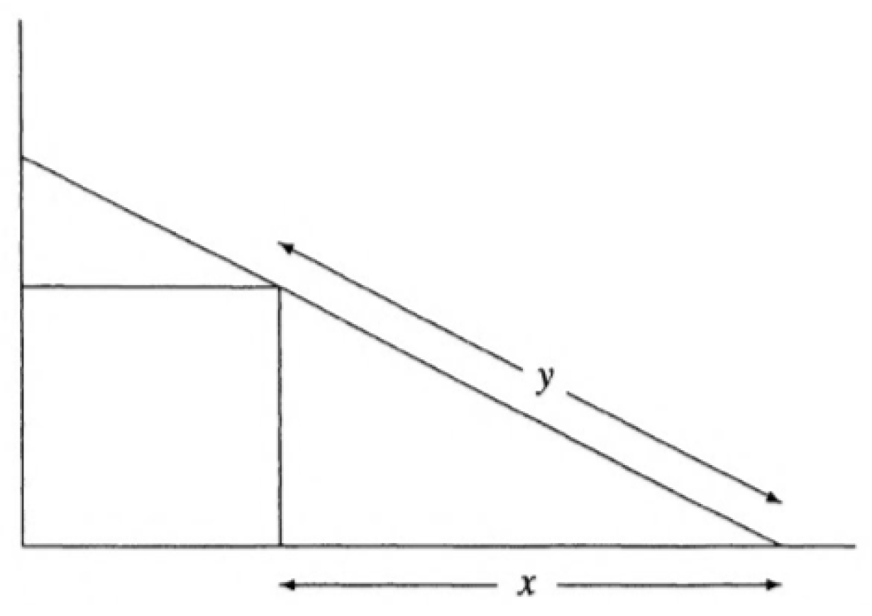
Example 2 (Beam Designing Model).

We consider a beam positioning problem (see [26]) where an r meter long beam is leaning against the edge of the cubical box with sides of length 1 m each, such that one of its ends touches the wall and the other touches the floor, as shown in Figure 1.

What should be the distance along the floor from the base of the wall to the bottom of the beam? Let y be the distance in meters along the beam from the floor to the edge of the box and let x be the distance in meters from the bottom of the box to the bottom of the beam. Then, for a given value of r, we have:

$$f_2\left(x\right)=x^4+4x^3-24x^2+16x+16=0.$$

The positive solution of the equation is a double root $x=2$. We consider the initial guess $x_0=1.7.$

Example 3 (The Shockley Diode Equation and Electric Circuit).

Let us consider an electric circuit consisting of a diode and a resistor. By Kirchoff’s voltage law, the source voltage drop $V_S$ is equal to the sum of the voltage drops across the diode $V_D$ and resistor $V_R:$

$$V_s=V_R+V_D.$$

(38)

Let the source voltage be $V_S=0.5$ V and from Ohm’s law:

$$V_R=RI.$$

(39)

Additionally, the voltage drop across the diode is given by the Shockley diode equation as follows:

$$I=I_S\left(e^{\frac{V_D}{n{V}_T}}-1\right),$$

(40)

where I is the diode current in amperes, $I_S$ is saturation current (amperes), n is the emission or ideality constant ($1\le n\le 2$ for silicon diode), and $V_D$ is the voltage applied across the diode. Solving Equation (40) for $V_D$ and using all the values in Equation (38), we obtain:

$$-0.5+RI+n{V}_{T}ln\left(\frac{I}{I_S}+1\right)=0$$

Now, for the given values of n, $V_T$, R and $I_S$, we have the following equation [27]:

$$-0.5+0.1I+1.4ln\left(I+1\right)=0.$$

Replacing I with x, we have

$$f_3\left(x\right)=-0.5+0.1x+1.4ln\left(x+1\right).$$

The true root of the equation is $0.389977198390077586586453532646$. We take $x_0=0.5.$

Example 4 (Eigenvalue Problem).

One of the challenging task of linear algebra is to calculate the eigenvalues of a large square matrix, especially when the required eigenvalues are the zeros of the characteristic polynomial obtained from the determinant of a square matrix of order greater than 4. Let us consider the following 9 × 9 matrix:

$$A=\frac{1}{8}\left[\begin{array}{ccccccccc}-12& 0& 0& 19& -19& 76& -19& 18& 437\\ -64& 24& 0& -24& 24& 64& -8& 32& 376\\ -16& 0& 24& 4& -4& 16& -4& 8& 92\\ -40& 0& 0& -10& 50& 40& 2& 20& 242\\ -4& 0& 0& -1& 41& 4& 1& 2& 25\\ -40& 0& 0& 18& -18& 104& -18& 20& 462\\ -84& 0& 0& -29& 29& 84& 21& 42& 501\\ 16& 0& 0& -4& 4& -16& 4& 16& -92\\ 0& 0& 0& 0& 0& 0& 0& 0& 24\end{array}\right].$$

The corresponding characteristic polynomial of matrix A is given as follows:

$$f_4\left(x\right)=x^9-29x^8+349x^7-2261x^6+8455x^5-17663x^4+15927x^3+6993x^2-24732x+12960.$$

(41)

The above function has one multiple zero at $\xi =3$ of multiplicity 4 with initial approximation $x_0=3.1$.

In Table 1, Table 2, Table 3 and Table 4, we show the numerical results obtained by applying the different methods for approximating the multiple roots of $f_1\left(x\right)-f_4\left(x\right)$. The obtained values confirm the theoretical results. From the tables, it can be observed that our proposed schemes $NS1$, $NS2$, and $NS3$ exhibit a better performance in approximating the multiple root of $f_1,$ $f_2$ and $f_4$ among other similar methods. Only in the case of the example for simple zeros Behl’s scheme BM1 is performing slightly better than the other methods.

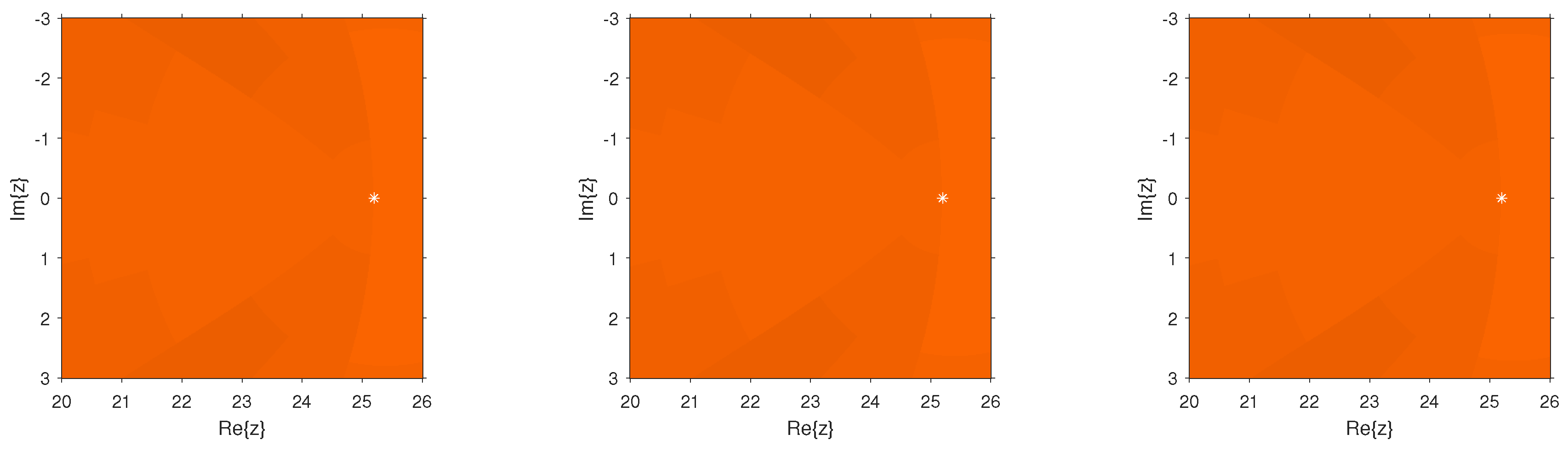
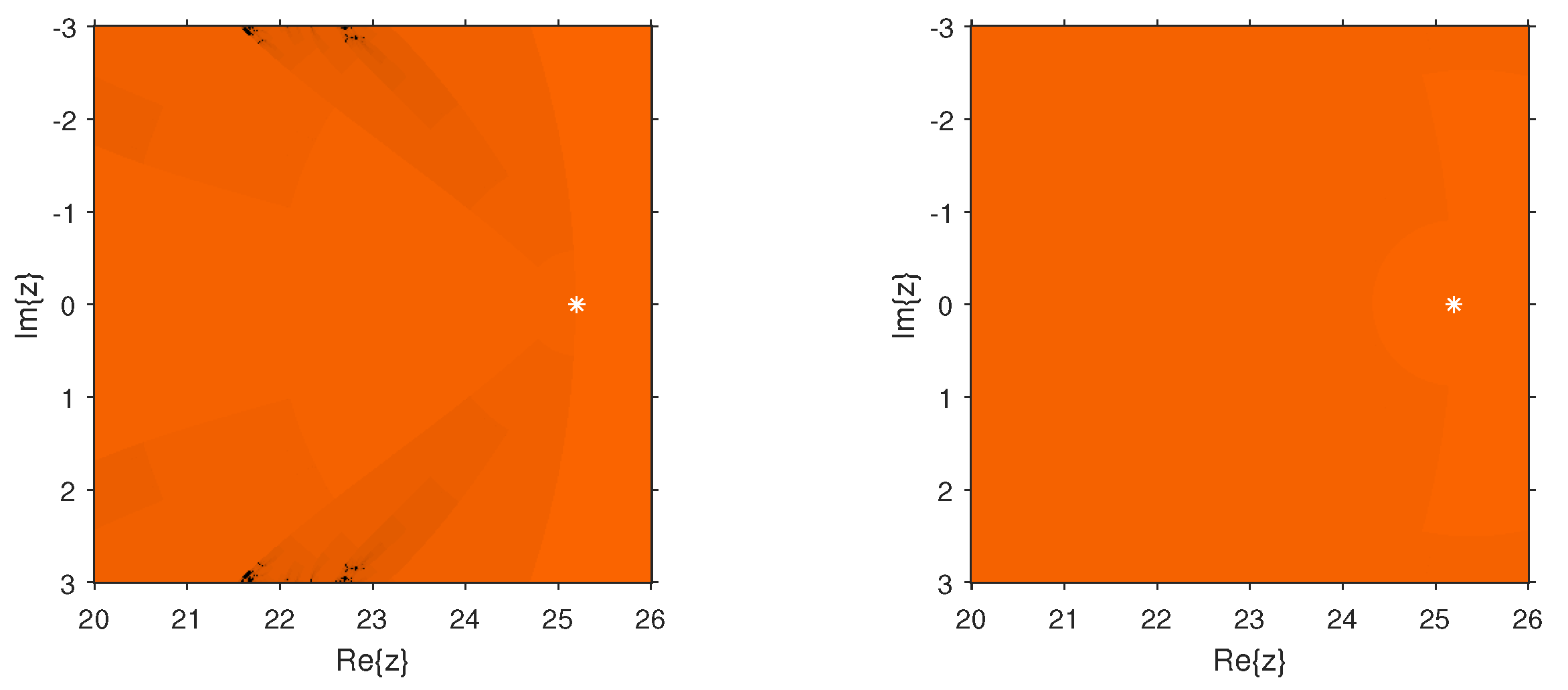
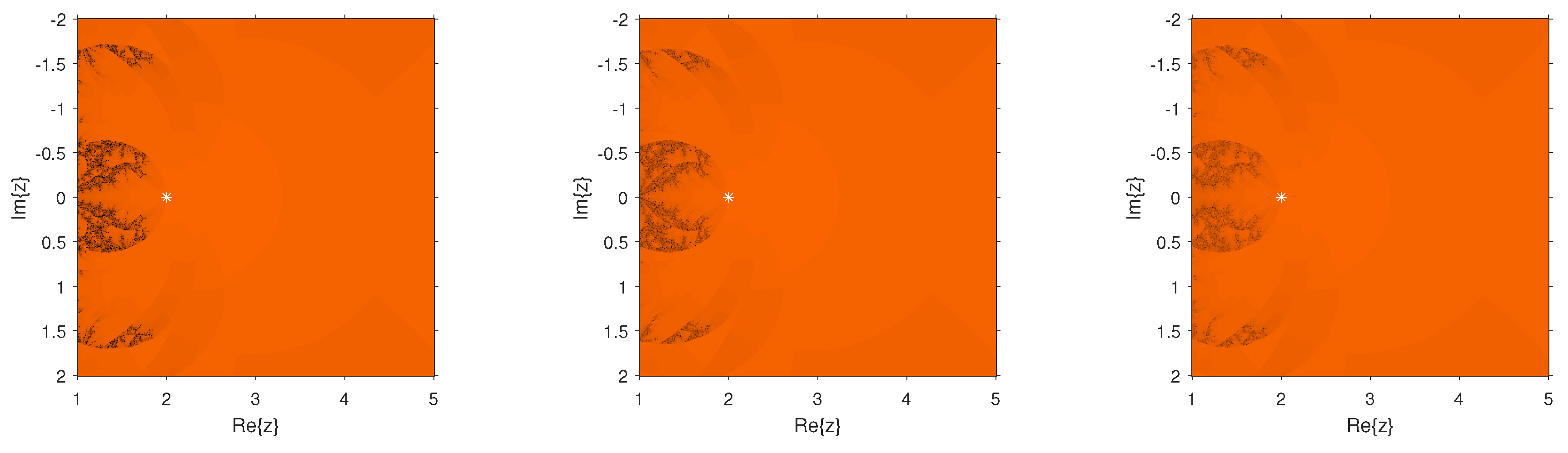
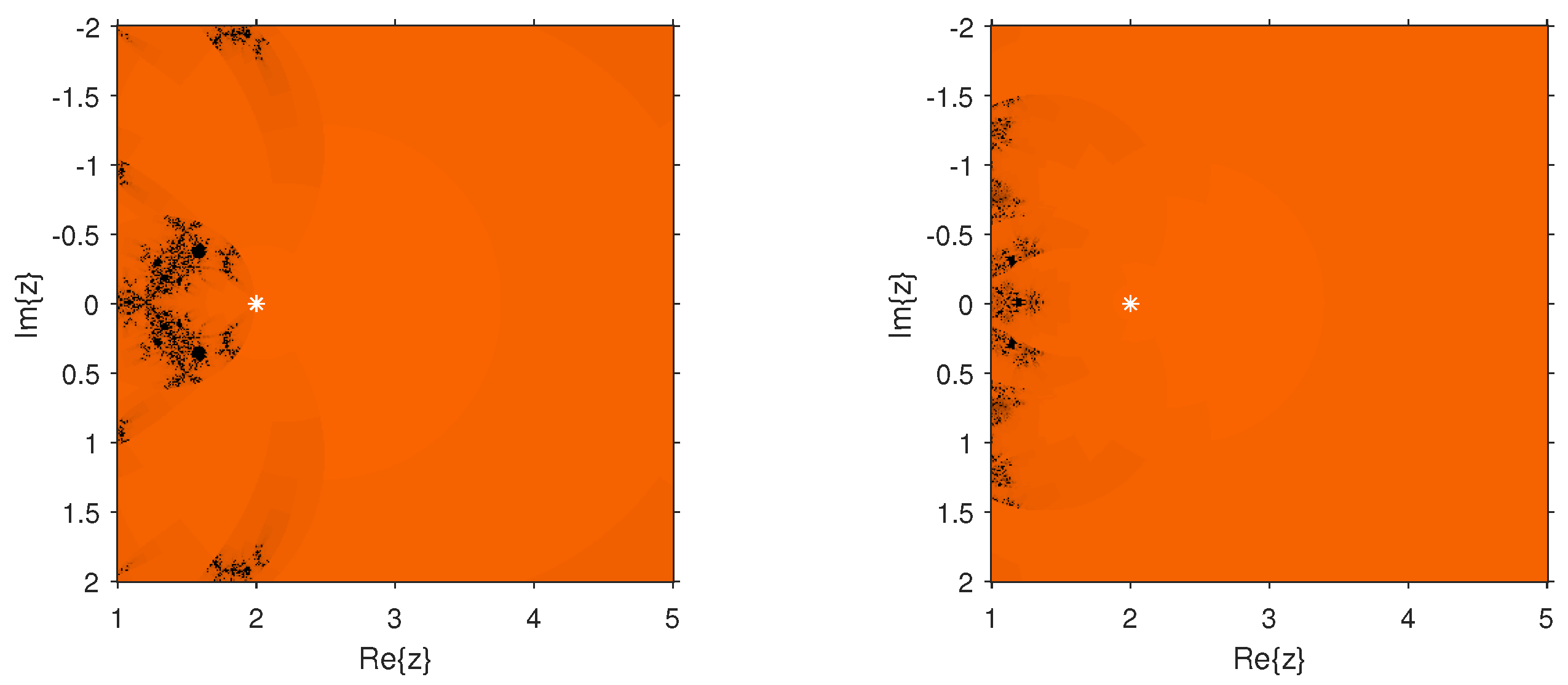
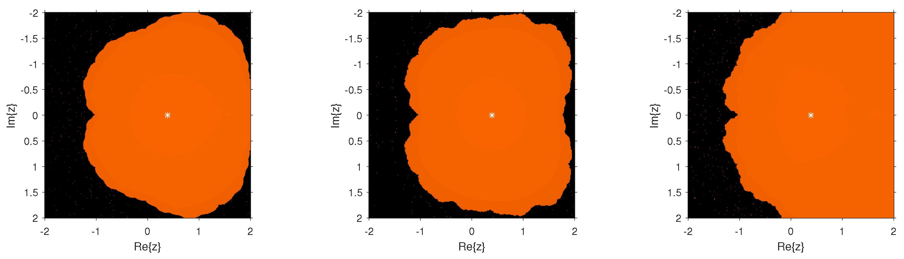
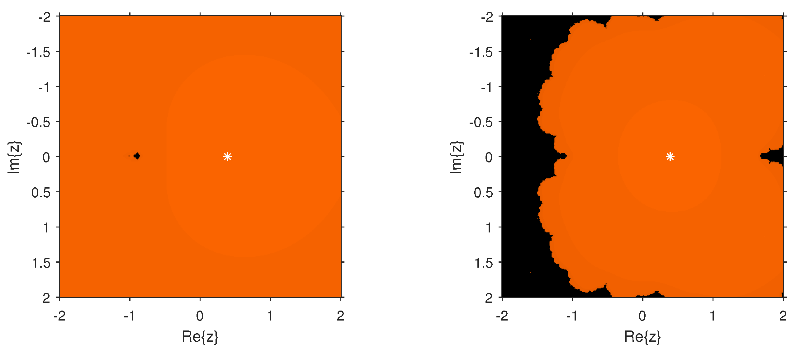
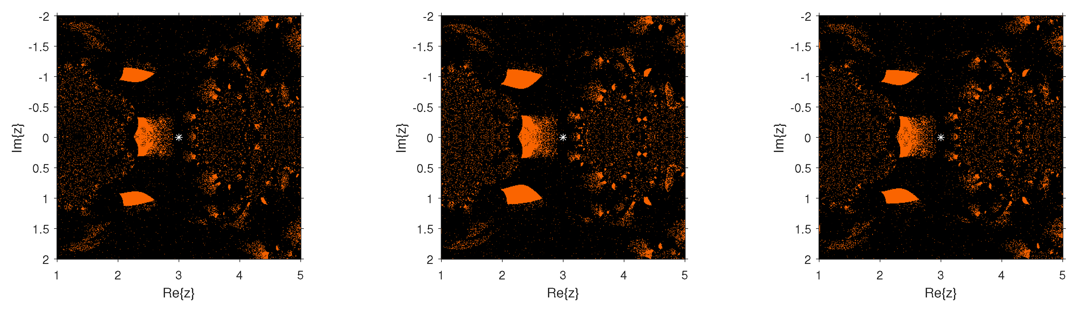
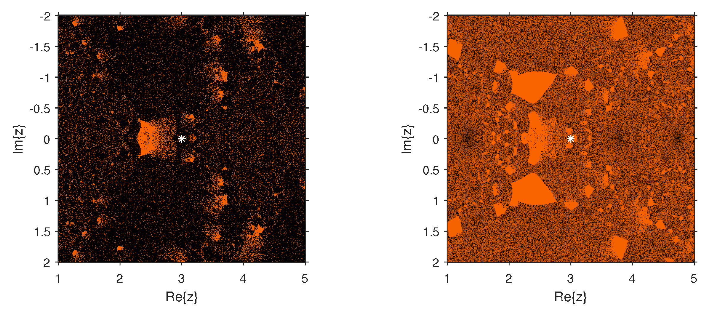
Dynamical Planes

The dynamical behavior of the test functions is presented in Figure 2, Figure 3, Figure 4, Figure 5, Figure 6, Figure 7, Figure 8 and Figure 9. The dynamical planes have been generated using the routines published in Reference [28]. We used a mesh of $400\times 400$ points in the region of the complex plane $[-100,100]\times [-100,100]$. We painted in orange the points whose orbit converged to the multiple root and in black those points whose orbit either diverged or converged to a strange fixed point or a cycle. We worked out with a tolerance of ${10}^{-3}$ and a maximum number of 80 iterations. The multiple root is represented in the different figures by a white star.

Figure 2, Figure 3, Figure 4, Figure 5, Figure 6, Figure 7, Figure 8 and Figure 9 study the convergence and divergence regions of the new schemes $NS1$, $NS2$, and $NS3$ in comparison with the other schemes of the same order. In the case of $f_1\left(x\right)$ and $f_2\left(x\right)$, we observed that the new schemes are more stable than $BM1$ and $BM2$ as they are almost divergence-free and also converge faster than $BM1$ and $BM2$ in their common regions of convergence. In the case of $f_3\left(x\right),$ $BM1$ performs better; however, $NS1$, $NS2$, and $NS3$ have an edge over $BM2$ for the region in spite of the analogous behavior to $BM2$, as the new schemes show more robustness. Similarly, in the case of $f_4\left(x\right),$ it can be clearly observed that the divergence region for $BM1$ is bigger than that for $NS1$, $NS2$, and $NS3$. Additionally, these schemes perform better than $BM2$ where they are convergent. The same behavior can be observed through the numerical comparison of these methods in Table 1, Table 2, Table 3 and Table 4. As a future extension, we shall be trying to construct a new optimal eighth-order method whose stability analysis can allow to choose the optimal weight function for the best possible results.

5. Conclusions

In this manuscript, a new general class of optimal eighth-order methods for solving nonlinear equations with multiple roots was presented. This family was obtained using the procedure of weight functions with two functions: One univariate and another depending on three variables. To reach this optimal order, some conditions on the functions and their derivatives must be imposed. Several special cases were selected and applied to different real problems, comparing their performance with that of other known methods of the same order of convergence. Finally, their dependence on initial estimations was analyzed from their basins of attraction.

References

1. Schroder, E. Uber unendlich viele Algorithmen zur Auflosung der Gleichungen. Math. Ann. 1870, 2, 317–365. [Google Scholar] [CrossRef]
2. Kung, H.T.; Traub, J.F. Optimal order of one-point and multipoint iteration. J. Assoc. Comput. Mach. 1974, 21, 643–651. [Google Scholar] [CrossRef]
3. Li, S.; Liao, X.; Cheng, L. A new fourth-order iterative method for finding multiple roots of nonlinear equations. Appl. Math. Comput. 2009, 215, 1288–1292. [Google Scholar]
4. Sharma, J.R.; Sharma, R. Modified Jarratt method for computing multiple roots. Appl. Math. Comput. 2010, 217, 878–881. [Google Scholar] [CrossRef]
5. Li, S.G.; Cheng, L.Z.; Neta, B. Some fourth-order nonlinear solvers with closed formulae for multiple roots. Comput. Math. Appl. 2010, 59, 126–135. [Google Scholar] [CrossRef] [Green Version]
6. Zhou, X.; Chen, X.; Song, Y. Constructing higher-order methods for obtaining the muliplte roots of nonlinear equations. J. Comput. Math. Appl. 2011, 235, 4199–4206. [Google Scholar] [CrossRef]
7. Sharifi, M.; Babajee, D.K.R.; Soleymani, F. Finding the solution of nonlinear equations by a class of optimal methods. Comput. Math. Appl. 2012, 63, 764–774. [Google Scholar] [CrossRef]
8. Soleymani, F.; Babajee, D.K.R.; Lofti, T. On a numerical technique forfinding multiple zeros and its dynamic. J. Egypt. Math. Soc. 2013, 21, 346–353. [Google Scholar] [CrossRef]
9. Soleymani, F.; Babajee, D.K.R. Computing multiple zeros using a class of quartically convergent methods. Alex. Eng. J. 2013, 52, 531–541. [Google Scholar] [CrossRef]
10. Liu, B.; Zhou, X. A new family of fourth-order methods for multiple roots of nonlinear equations. Non. Anal. Model. Cont. 2013, 18, 143–152. [Google Scholar]
11. Zhou, X.; Chen, X.; Song, Y. Families of third and fourth order methods for multiple roots of nonlinear equations. Appl. Math. Comput. 2013, 219, 6030–6038. [Google Scholar] [CrossRef]
12. Thukral, R. A new family of fourth-order iterative methods for solving nonlinear equations with multiple roots. J. Numer. Math. Stoch. 2014, 6, 37–44. [Google Scholar]
13. Behl, R.; Cordero, A.; Motsa, S.S.; Torregrosa, J.R. On developing fourth-order optimal families of methods for multiple roots and their dynamics. Appl. Math. Comput. 2015, 265, 520–532. [Google Scholar] [CrossRef]
14. Hueso, J.L.; Martínez, E.; Teruel, C. Determination of multiple roots of nonlinear equations and applications. J. Math. Chem. 2015, 53, 880–892. [Google Scholar] [CrossRef]
15. Behl, R.; Cordero, A.; Motsa, S.S.; Torregrosa, J.R.; Kanwar, V. An optimal fourth-order family of methods for multiple roots and its dynamics. Numer. Algor. 2016, 71, 775–796. [Google Scholar] [CrossRef]
16. Neta, B. Extension of Murakami’s high-order non-linear solver to multiple roots. Int. J. Comput. Math. 2010, 87, 1023–1031. [Google Scholar] [CrossRef]
17. Geum, Y.H.; Kim, Y.I.; Neta, B. A class of two-point sixth-order multiple-zero finders of modified double-Newton type and their dynamics. Appl. Math. Comput. 2015, 270, 387–400. [Google Scholar] [CrossRef] [Green Version]
18. Geum, Y.H.; Kim, Y.I.; Neta, B. A sixth-order family of three-point modified Newton-like multiple-root finders and the dynamics behind their extraneous fixed points. Appl. Math. Comput. 2016, 283, 120–140. [Google Scholar] [CrossRef] [Green Version]
19. Behl, R.; Cordero, A.; Motsa, S.S.; Torregrosa, J.R. An eighth-order family of optimal multiple root finders and its dynamics. Numer. Algor. 2017. [Google Scholar] [CrossRef]
20. Zafar, F.; Cordero, A.; Rana, Q.; Torregrosa, J.R. Optimal iterative methods for finding multiple roots of nonlinear equations using free parameters. J. Math. Chem. 2017. [Google Scholar] [CrossRef]
21. Geum, Y.H.; Kim, Y.I.; Neta, B. Constructing a family of optimal eighth-order modified Newton-type multiple-zero finders along with the dynamics behind their purely imaginary extraneous fixed points. J. Comput. Appl. Math. 2018, 333, 131–156. [Google Scholar] [CrossRef]
22. Behl, R.; Zafar, F.; Alshomrani, A.S.; Junjua, M.; Yasmin, N. An optimal eighth-order scheme for multiple zeros of univariate function. Int. J. Comput. Math. 2018, 15. [Google Scholar] [CrossRef]
23. Behl, R.; Alshomrani, A.S.; Motsa, S.S. An optimal scheme for multiple roots of nonlinear equations with eighth-order convergence. J. Math. Chem. 2018. [Google Scholar] [CrossRef]
24. Jay, L.O. A note on Q-order of convergence. BIT Numer. Math. 2001, 41, 422–429. [Google Scholar] [CrossRef]
25. Edelstein-Keshet, L. Differential Calculus for the Life Sciences; Univeristy of British Columbia: Vancouver, BC, Canada, 2017. [Google Scholar]
26. Zachary, J.L. Introduction to Scientific Programming: Computational Problem Solving Using Maple and C; Springer: New York, NY, USA, 2012. [Google Scholar]
27. Khoury, R. Douglas Wilhelm Harder, Numerical Methods and Modelling for Engineering; Springer International Publishing: Berlin, Germany, 2017. [Google Scholar]
28. Chicharro, F.I.; Cordero, A.; Torregrosa, J.R. Drawing dynamical and parameters planes of iterative families and methods. Sci. World J. 2013, 2013, 780153. [Google Scholar] [CrossRef] [PubMed]
Figure 1. Beam positioning problem.
Mathematics 06 00310 g001
Figure 2. Dynamical planes of the methods N S 1 (Left), N S 2 (Center), and N S 3 (Right) for f 1 ( x ) .
Mathematics 06 00310 g002
Figure 3. Dynamical planes of the methods B M 1 (Left) and B M 2 (Right) for f 1 ( x ) .
Mathematics 06 00310 g003
Figure 4. Dynamical planes of the methods N S 1 (Left), N S 2 (Center), and N S 3 (Right) for f 2 ( x ) .
Mathematics 06 00310 g004
Figure 5. Dynamical planes of the methods B M 1 (Left) and B M 2 (Right) on f 2 ( x ) .
Mathematics 06 00310 g005
Figure 6. Dynamical planes of the methods N S 1 (Left), N S 2 (Center), and N S 3 (Right) for f 3 ( x ) .
Mathematics 06 00310 g006
Figure 7. Dynamical planes of the methods B M 1 (Left) and B M 2 (Right) for f 3 ( x ) .
Mathematics 06 00310 g007
Figure 8. Dynamical planes of the methods N S 1 (Left), N S 2 (Center), and N S 3 (Right) on f 4 ( x ) .
Mathematics 06 00310 g008
Figure 9. Dynamical planes of the methods B M 1 (Left) and B M 2 (Right) for f 4 ( x ) .
Mathematics 06 00310 g009