A Novel Simple Particle Swarm Optimization Algorithm for Global Optimization


Abstract
:1. Introduction
- Principle study: The inertia weight factor, which adjusts the ability of PSO algorithm in local and global search was introduced by Shi and Eberhart [32], effectively avoiding falling into local optimum for PSO. Shi and Eberhart provided a way of thinking for future improvement. In 2001, Parsopoulos and Vrahatis [33]’s research showed that basic PSO can work effectively and stably in noisy environments, and in many cases, the presence of noise can also help PSO avoid falling into local optimum. The basic PSO was introduced for continuous nonlinear function [21,22]. However, because the basic PSO is easy to fall into the local optima, local PSO(LPSO) [34] was introduced in 2002. Clerc and Kennedy [35] proposed a constriction factor to enhance the explosion, stability, and convergence in a multidimensional complex space. Xu and Yu [36] used the super-martingale convergence theorem to analyze the convergence of the particle swarm optimization algorithm. The results showed that the particle swarm optimization algorithm achieves the global optima in probability and the quantum-behaved particle swarm optimization (QPSO) [37] has also been proved to have global convergence.
- Parameter setting: A particle swarm optimization with fitness adjustment parameters (PSOFAB) [38], based on the fitness performance, was proposed in order to converge to an approximate optimal solution. The experimental results were analyzed by the Wilcoxon signed rank test, and its analysis showed that PSOFAP [38] is effective in increasing the convergence speed and the solution quality. It accurately adapts the parameter value without performing parametric sensitivity analysis. The inertia weight of the hybrid particle swarm optimization incorporating fuzzy reasoning and weighted particle (HPSOFW) [39] is changed based on defuzzification output. The chaotic binary PSO with time-varying acceleration coefficients (CBPSOTVAC) [40] using 116 benchmark problems from the OR-Library to test has time-varying acceleration coefficients for the multidimensional knapsack problem. A self-organizing hierarchical PSO [41] also uses time-varying acceleration coefficients.
- Topology improvement: In 2006, Kennedy and Mendes [42] explained the neighborhood topologies in fully informed and best-of-neighborhood particle swarms in detail. A dynamic multiswarm particle swarm optimizer (DMSPSO) [43] was proposed, and it adopts a neighborhood topology including a random selection of small swarms with small neighborhood. Moreover, the regrouped group is dynamic and randomly assigned. In 2014, FNNPSO [44] use Fluid Neural Networks (FNNs) to create a dynamic neighborhood mechanism. The results showed that FNNPSO can outperform both the standard PSO algorithm and PCGT-PSO. Sun and Li proposed a two-swarm cooperation particle swarm optimization (TCPSO) [45] that used the slave swarm and the master swarm to exchange the information, which is beneficial for enhancing the convergence speed and maintaining the swarm diversity in TCPSO, and particles update the next particle with information from its neighboring particles, rather than its own history best solution and current velocity. This strategy makes the particles of the subordinate group more inclined to local optimization, thus accelerating convergence. Inspired by the cluster reaction of the starlings, Netjinda et al. [46] used the collective response mechanism to influence the velocity and position of the current particle by seven adjacent ones, thereby increasing the diversity of the particles. A nonparametric particle swarm optimization (NP-PSO) [47] combines local and global topologies with two quadratic interpolation operations to enhance the PSO capability without tuning any algorithmic parameter.
- Updating formula improvement: Mendes [48] changed the PSO’s velocity and personal best solution updating formula and proposed a fully informed particle swarm (FIPS) algorithm to make good use of the whole entire swarm. Mendes [49] proposed a Comprehensive learning particle swarm optimizer (CLPSO) whose velocity updating formula eliminates the influence from global best solution to to suit the multimodal functions, and CLPSO uses two tournament-selected particles to help particles study better case during iteration. The results showed that CLPSO performs better than other PSO variants for multimodal problems. A learning particle swarm optimization (*LPSO) algorithm [50] was proposed with a new framework that changed the velocity updating formula so as to organically hybridize PSO with another optimization technique. *LPSO is composed of two cascading layers: exemplar generation and a basic PSO algorithm updating method. A new global particle swarm optimization (NGPSO) algorithm [51] uses a new position updating equation that relies on the global best particle to guide the searching activities of all particles. In the latter part of the NGPSO search, the random distribution based on uniform distribution is used to increase the particle swarm diversity and avoid premature convergence. Kiran proposed a PSO with a distribution-based position update rule (PSOd) [52] whose position updating formula is combined with three variables.
- Hybrid mechanism: In 2014, Wang et al. [53] proposed a series of chaotic particle-swarm krill herd (CPKH) algorithms for global numerical optimization. The CPKH is a hybird Krill herd (KH) [54] algorithm with APSO [55] which has a mutation operator and chaotic theory. This hybrid algorithm, which with an appropriate chaotic map performs superiorly to the standard KH and other population-based optimization, has quick exploitation for solution. DPSO [56] is a accelerated PSO (APSO) [55] algorithm hybridized with a DE algorithm mutation operator. It has a superior performance due to combining the advantages from both APSO and DE. Wang et al., finally, studied and analyzed the effect of the DPSO parameters on convergence and performance by detailed parameter sensitivity studies. In he hybrid learning particle swarm optimizer with genetic disturbance (HLPSO-GD) [57], the genetic disturbance is used to cross the corresponding particle in the external archive, and new individuals are generated, which will improve the swarm’s ability to escape from the local optima. Gong et al. proposed a genetic learning particle swarm optimization (GLPSO) algorithm that uses genetic evolution to breed promising exemplars based on *LPSO [50] enhancing the global search ability and search efficiency of PSO. PSOTD [58] namely a particle swarm optimization algorithm with two differential mutation, which has a novel structure with two swarms and two layers including bottom layer and top layer, was proposed for 44 benchmark functions. HNPPSO [59] is a novel particle swarm optimization combined with a multi-crossover operation, a vertical crossover, and an exemplar-based learning strategy. To deal with production scheduling optimization in foundry, a hybrid PSO combined the SA [7] algorithm [60] was proposed.
- Practical application: Zou et al. used NGPSO [51] to solve the economic emission dispatch (EED) problems and the results showed that NGPSO is the most efficient approach for solving the economic emission dispatch (EED) problems. PS-CTPSO [61] based on the predatory search strategy was proposed to do with web service combinatorial optimization, which is an NP problem, and it improves overall ergodicity. To improve the changeability of ship inner shell, IPSO [62] was proposed for a 50,000 DWT product oil tanker. MBPSO [63] was proposed for sensor management of LEO constellation to the problem of utilizing a low Earth orbit (LEO) infrared constellation in order to track the midcourse ballistic missile. GLNPSO [64] is for a capacitated Location-Routing Problem. The particle swarm algorithm is also applied to many other practical problems e.g., PID (Proportion Integration Differentiation) controller [65], optimal strategies of energy management integrated with transmission control for a hybrid electric vehicle [66], production scheduling optimization in foundry [60], etc.
2. Related Works
2.1. The Basic PSO
- Step 1:
- Initialize the population randomly. Set the maximum number of iterations, population size, inertia weight, cognitive factors, social factors, position limits and the maximum velocity limit.
- Step 2:
- Calculate the fitness of each particle according to fitness function or models.
- Step 3:
- Compare the fitness of each particle with its own history best solution . If the fitness is smaller than , the smaller value is assigned to , otherwise, is reserved. Then, the fitness is compared with the global best solution , and the method is the same as selecting .
- Step 4:
- Step 5:
- Check if the theoretical optimum is reached, output the value and stop the operation; otherwise, return to Step 2 (Section 2.1) until it reaches the theoretical optima or peaks the maximum number of iterations.
2.2. The PSO with a Distribution-Based Position Update Rule
- Step 1:
- The population is initialized randomly.
- Step 2:
- The fitness is calculated and compared to get the best individual history solution and the best global one.
- Step 3:
- Equation (5) is used to update the particle position that is limited in the upper and lower limits.
- Step 4:
- If the termination condition is met, the best solution is reported.
2.3. A Hybrid PSO with Sine Cosine Acceleration Coefficients
- Step 1:
- The population is initialized randomly.
- Step 2:
- The reverse population of the initial population is calculated by Equation (9)In this equation, and are initial population and reverse population, respectively. and are combined the upper and lower limits of particles position i.e., the solution space boundary.
- Step 3:
- Fitness values of those two populations are sorted, and the best half is used as the initial population. Then, the and are obtained by comparing.
- Step 4:
- Step 5:
- Updating the particle velocity and position, use Equations (1) and (12). The particle position updating formula is as follows:and are the dynamic weights that control position and velocity terms. Its formula is like Equation (13). is a random value between 0 and l:In this formula, is the particle fitness value, and is the average one.
- Step 6:
- The iteration is ended if end condition is reached. Otherwise, it comes back to Step 2 (Section 2.3).
2.4. A Two-Swarm Cooperative PSO
- Step 1:
- Initialization. Initialize the slave swarm and the master swarm’s velocity and position randomly.
- Step 2:
- Calculate the fitness of these two swarms and get the , , and . The first two come from the slave swarm and the last two come from the master swarm.
- Step 3:
- Reproduction and updating.
- Step 3.1:
- Update the slave swarm by Equations (14) and (15). Ensure that velocity and position are within the limits:S in these two formulas means that this variable from the slave swarm, except in Equation (14) from the master swarm. Finally, we will get the . is randomly chosen from the neighberhood of the according to Equation (16) [42]:l is the size of neighborhood. Sun and Li found that the size of neighborhood equal to 2 is best in their experiments.
- Step 3.2:
- Update the master swarm by Equations (17) and (18). Ensure that velocity and position are within the limits:M here means that this variable is from the master swarm. In the end of Step 3.2 (Section 2.4), wil be obtained for the next iteration.
- Step 4:
- Get the optima if it meets the termination condition; otherwise, go to Step 2 (Section 2.4).
3. SPSO, SPSOC, SPSORC
3.1. Simple PSO
- Step 1:
- The maximum generation, population number, inertia weight, learning factor are set up. Population is initialized.
- Step 2:
- Fitness is calculated according to the function.
- Step 3:
- Every particle compares with its history best solution to get the and compares with the global best one to get the .
- Step 4:
- Particle position is updated by Equation (21).
- Step 5:
- If the theoretical optimal value is not found, the program returns to Step 2 (Section 3.1); otherwise, the program stops.
3.2. SPSO with Confidence Term
3.3. SPSOC Based on Random Weight
4. Experimental Study and Results Analysis
4.1. Benchmark Functions
4.2. Parameters Setting and Simulation Environment
4.3. Discussion on Improvement Necessity For SPSO
4.4. Discussion on Weight Selection for SPSOC
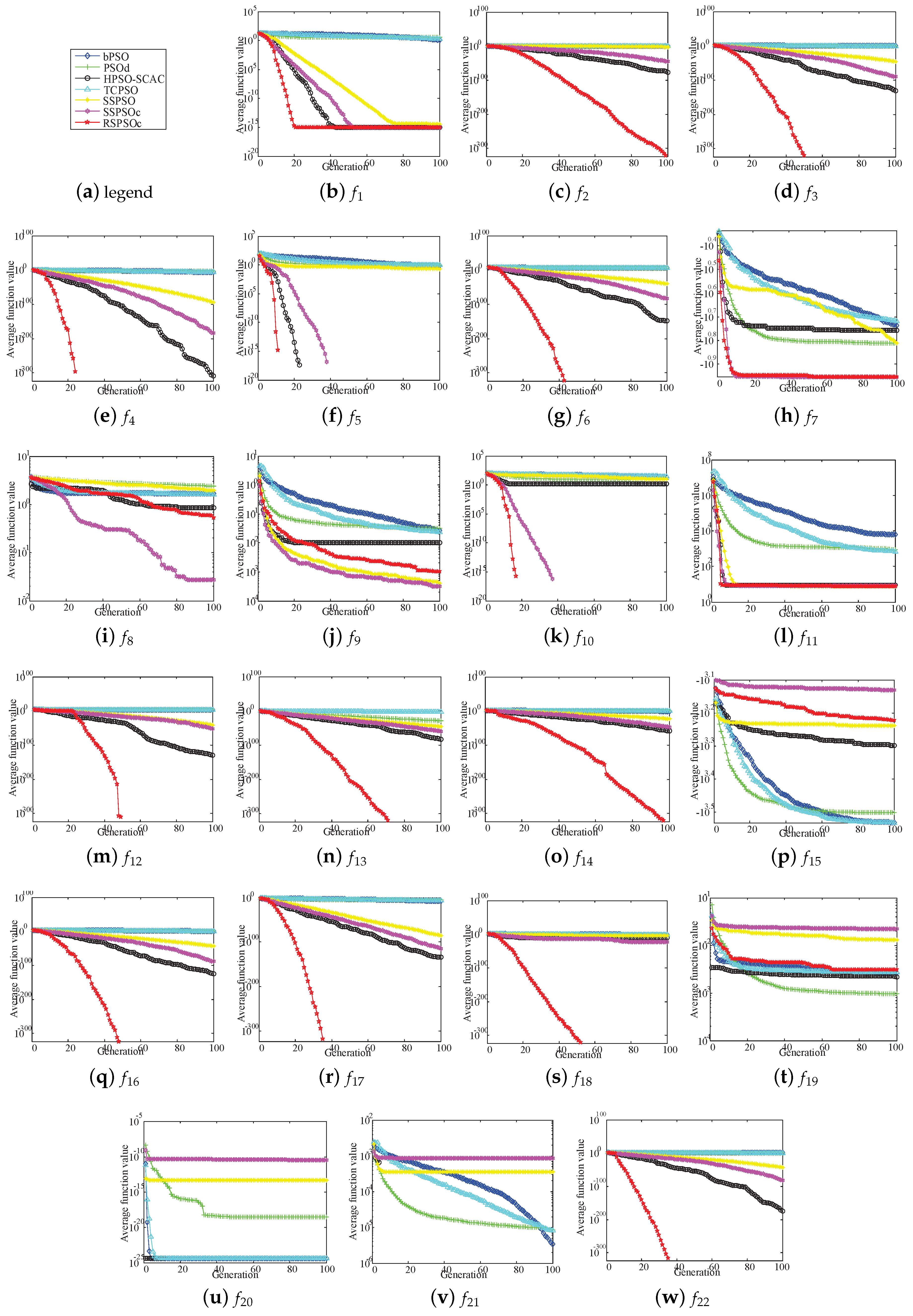
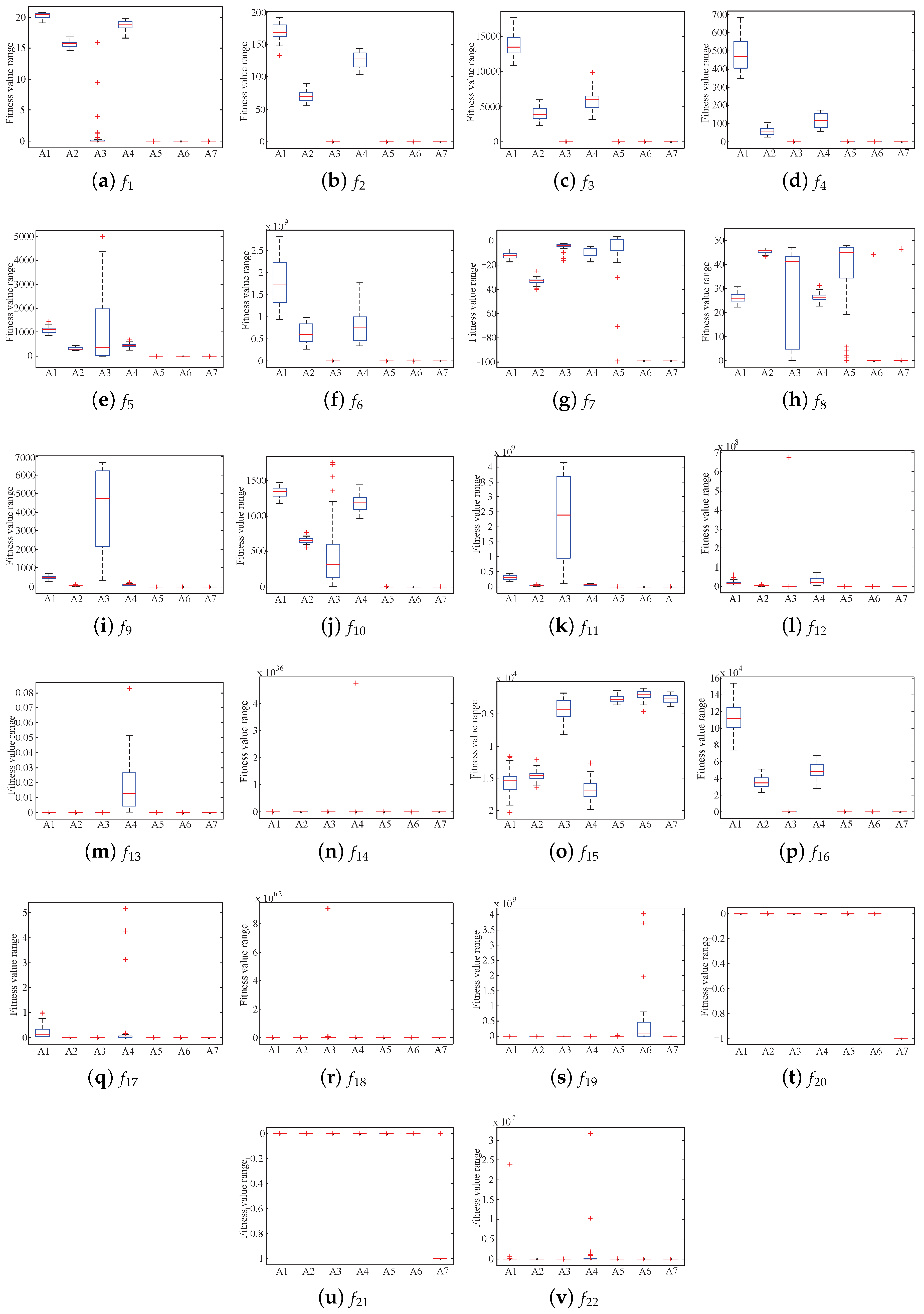
4.5. Comparison and Analysis with Other PSOs
4.5.1. Different Dimensional Experiments and t-Test Analysis
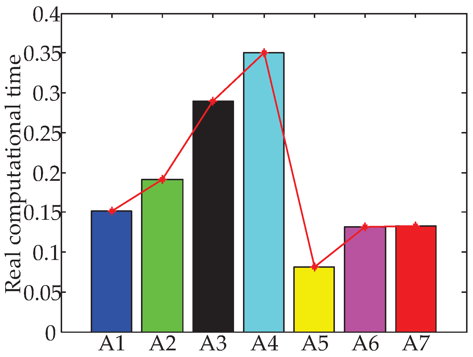
4.5.2. Algorithm Complexity Analysis
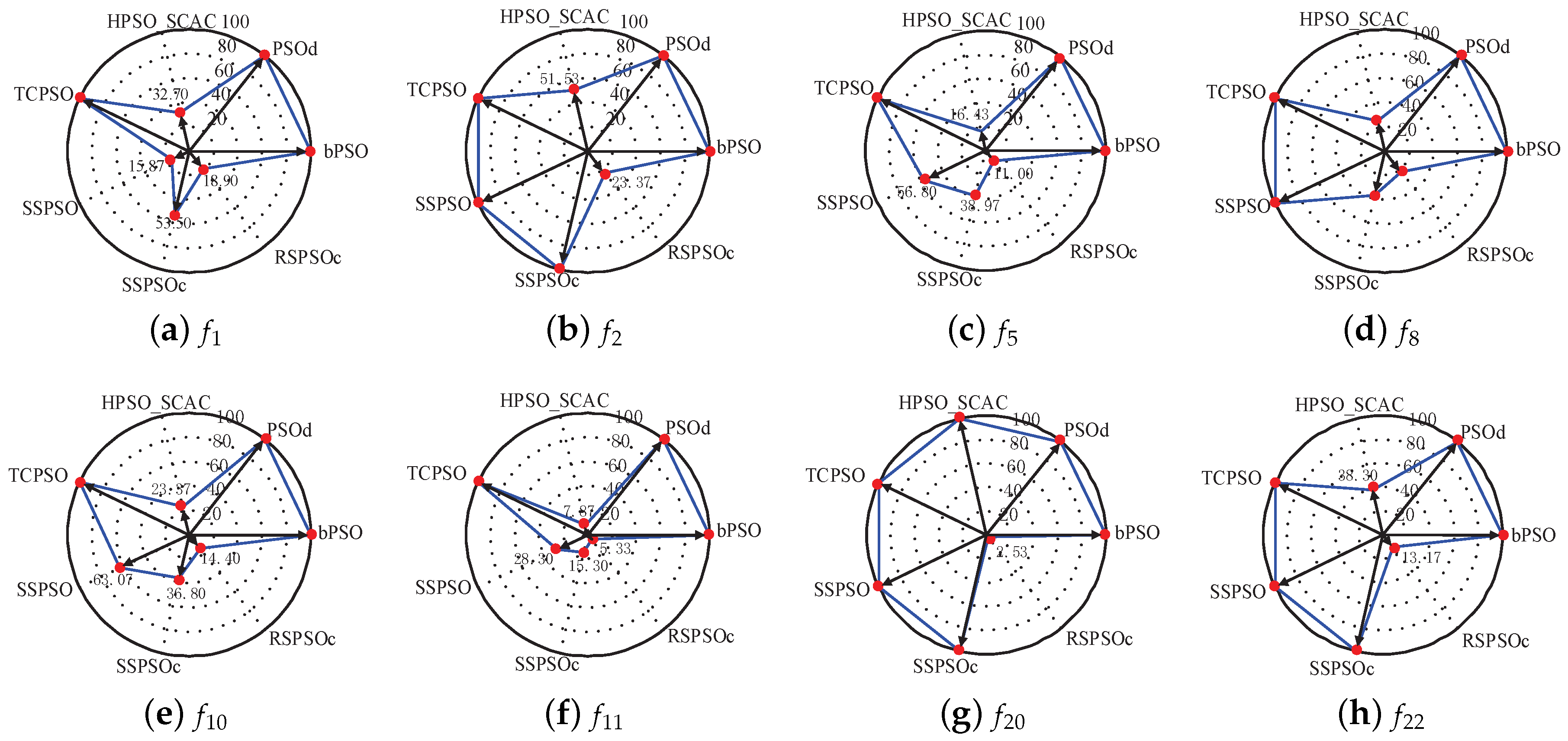
4.5.3. Success Rate and Average Iteration Times
5. Conclusions
Author Contributions
Funding
Acknowledgments
Conflicts of Interest
Abbreviations
| PSO | Particle Swarm Optimization |
| bPSO | The basic PSO [21,22] |
| PSOd | A distribution-based update rule for PSO [52] |
| HPSOscac | A hybrid PSO with sine cosine acceleration coefficients [67] |
| TCPSO | A two-swarm cooperative PSO [45] |
| SPSO | Simple PSO |
| SPSOC | Simple PSO with Confidence Term |
| SPSORC | Simple PSO based on Random weight and Confidence term |
| Particle velocity | |
| Particle position | |
| Personal historical best solution | |
| Global best solution | |
| Inertia weight | |
| The maximum weight | |
| The minimum wight | |
| Self-cognitive factor | |
| Social communication factor | |
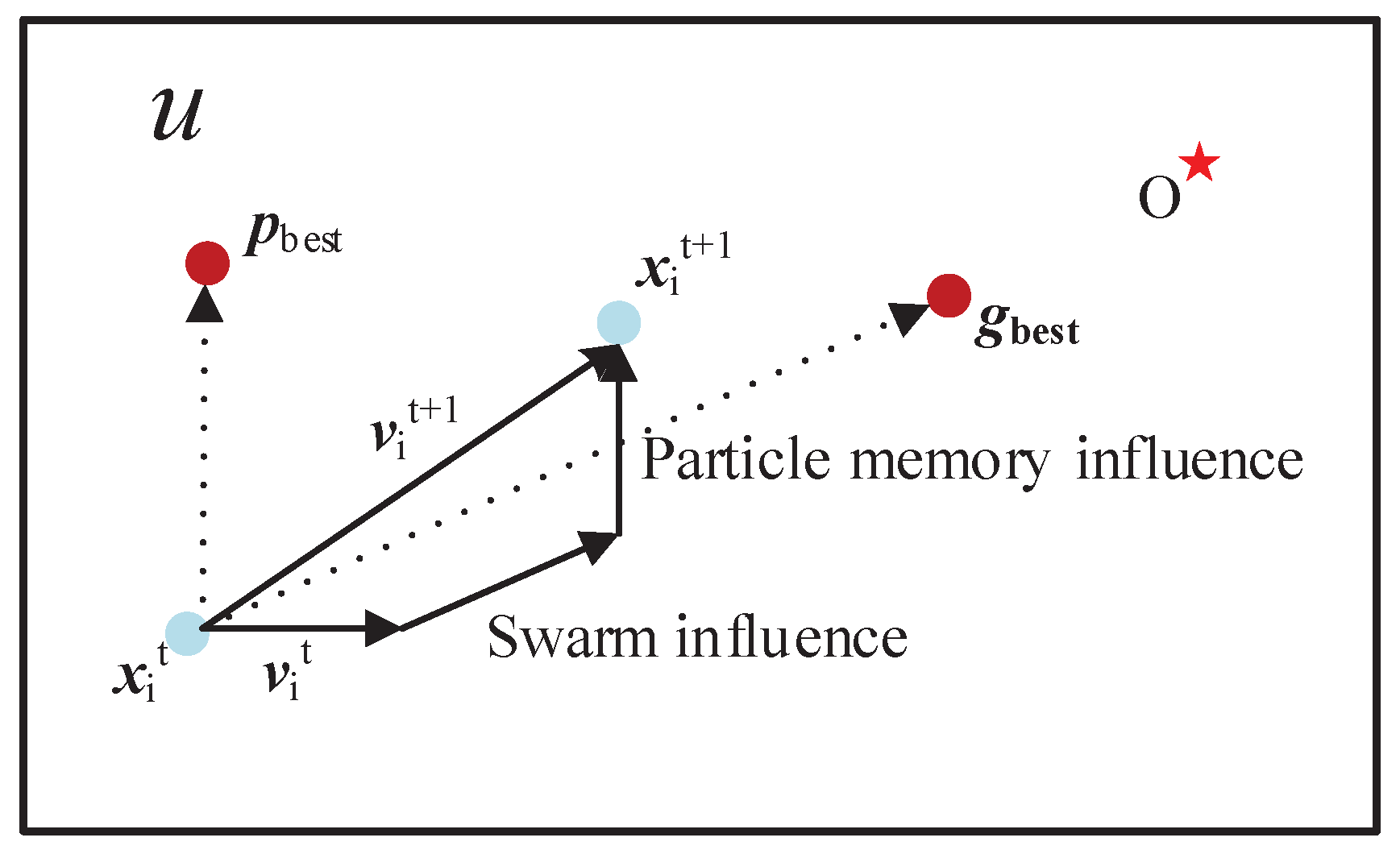
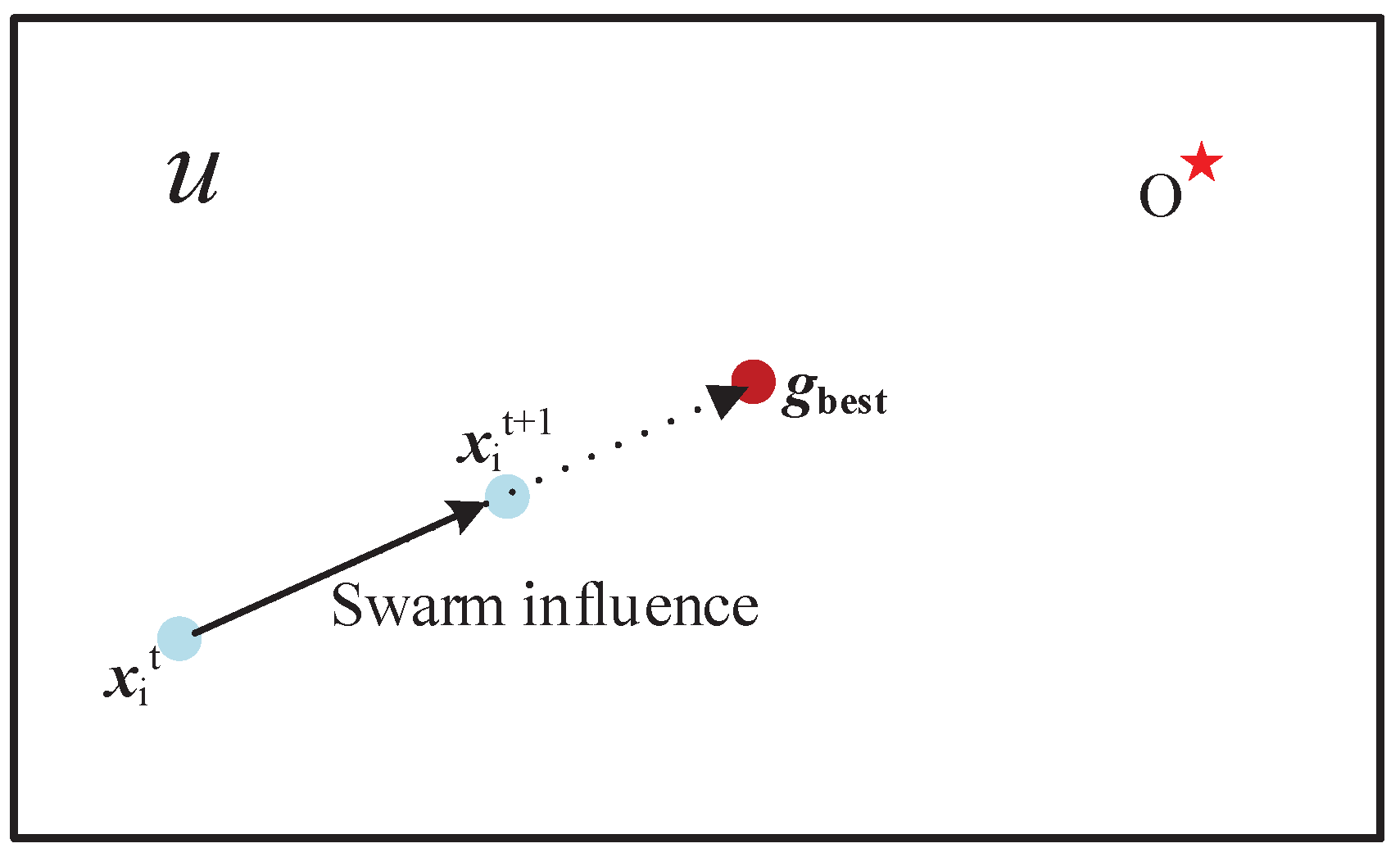
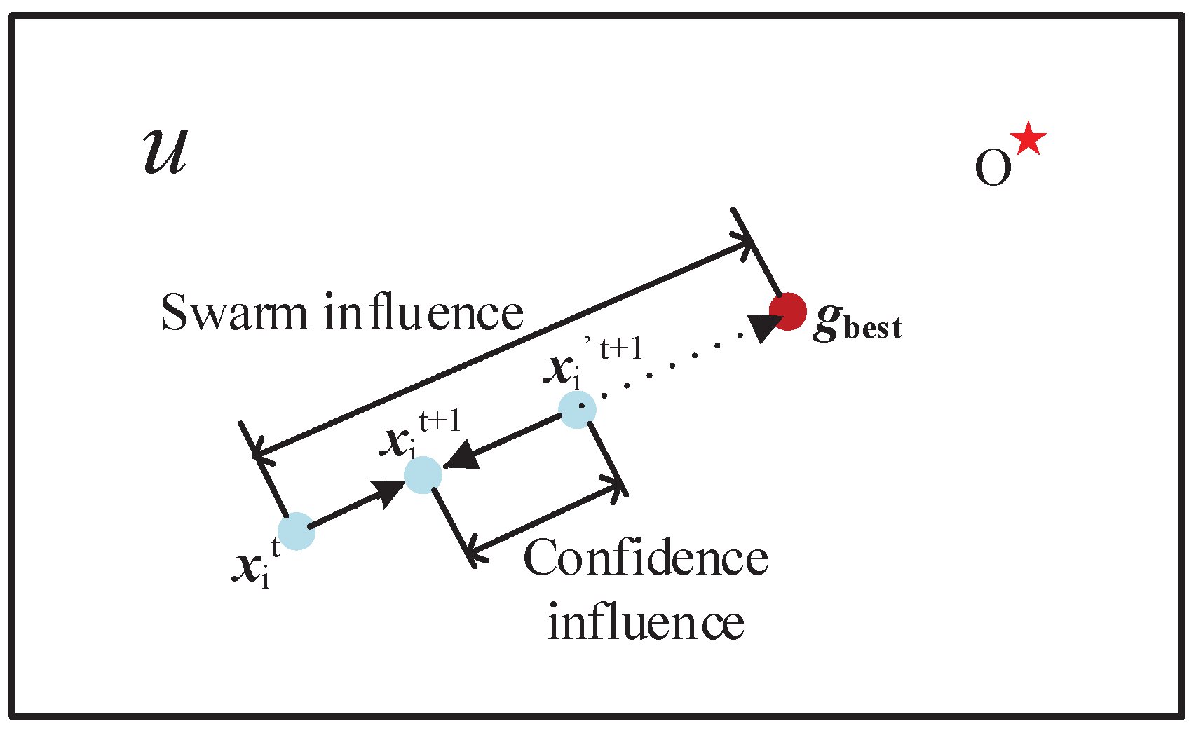
| U (in Figure 1, Figure 2 and Figure 3) | Solution space of a function |
| O (in Figure 1, Figure 2 and Figure 3) | The theoretical optima of a function |
| i | The current particle |
| n | The current dimension |
| N | The maximum dimension |
| t | The current generation |
| T | The upper limit of generation |
| The number of times that algorithm search for problem | |
| m | Population size |
| min | The minimum values from the optima in which algorithms search for the problem 30 times |
| mean | The average values for the optima in which algorithms search for the problem 30 times |
| std | The average values for the optima in which algorithms search for the problem 30 times |
| ttest (in Table 6) | t-test results |
| AIT (in Section 4.5.2) | Average iteration times |
| SR (in Section 4.5.2) | Success rate |
| A1–A7 (in Figure 5 and Figure 6) | bPSO, PSOd, HPSOscac, TCPSO, SPSO, SPSOC and SPSORC, respectively |
Appendix A. Benchmark Function Appendix

| Instance | Expression | Domain | Analytical Solution | Accuracy (50) |
|---|---|---|---|---|
| Ackley’s Path Function | ||||
| Alpine Function | ||||
| Axis Parallel Hyperellipsoid | ||||
| De Jong’s Function 4 (no noise) | ||||
| Girewank Problem | ||||
| High Conditioned Elliptic Function | ||||
| Inverted Cosine Wave Function | ||||
| Pathological Function | ||||
| Quartic Function, i.e, noise | rand | |||
| Rastrigin Problem | ||||
| Rosenbrock Problem | ||||
| Schwefel’s Problem 1.2 | ||||
| Schwefel’s Problem 2.21 | ||||
| Schwefel’s Problem 2.22 | ||||
| Schwefel’s Problem 2.26 | N | |||
| Sphere Function | ||||
| Sum of Different Power Function | ||||
| Xin–She Yang 1 | rand | |||
| Xin–She Yang 2 | ||||
| Xin–She Yang 3 | ||||
| Xin–She Yang 4 | ||||
| Zakharov Function |
References
- Denysiuk, R.; Gaspar-Cunha, A. Multiobjective Evolutionary Algorithm Based on Vector Angle Neighborhood. Swarm Evol. Comput. 2017, 37, 663–670. [Google Scholar] [CrossRef]
- Wang, G.G. Moth search algorithm: A bio-inspired metaheuristic algorithm for global optimization problems. Memet. Comput. 2016, 10, 1–14. [Google Scholar] [CrossRef]
- Feng, Y.H.; Wang, G.G. Binary moth search algorithm for discounted 0–1 knapsack problem. IEEE Access 2018, 6, 10708–10719. [Google Scholar] [CrossRef]
- Grefenstette, J.J. Genetic algorithms and machine learning. Mach. Learn. 1988, 3, 95–99. [Google Scholar] [CrossRef]
- Dorigo, M.; Gambardella, L.M. Ant colony system: A cooperative learning approach to the traveling salesman problem. IEEE Trans. Evol. Comput. 1997, 1, 53–66. [Google Scholar] [CrossRef]
- Storn, R.; Price, K. Differential Evolution—A Simple and Efficient Heuristic for global Optimization over Continuous Spaces. J. Glob. Optim. 1997, 11, 341–359. [Google Scholar] [CrossRef]
- Kirkpatrick, S.; Vecchi, M.P. Optimization by simulated annealing. Science 1983, 220, 671–680. [Google Scholar] [CrossRef] [PubMed]
- Wang, G.G.; Gandomi, A.H.; Alavi, A.H.; Deb, S. A multi-stage krill herd algorithm for global numerical optimization. Int. J. Artif. Intell. Tools 2016, 25, 1550030. [Google Scholar] [CrossRef]
- Wang, G.G.; Deb, S.; Gandomi, A.H.; Alavi, A.H. Opposition-based krill herd algorithm with Cauchy mutation and position clamping. Neurocomputing 2016, 177, 147–157. [Google Scholar] [CrossRef]
- Wang, G.G.; Gandomi, A.H.; Alavi, A.H. An effective krill herd algorithm with migration operator in biogeography-based optimization. Appl. Math. Model. 2014, 38, 2454–2462. [Google Scholar] [CrossRef]
- Wang, G.G.; Guo, L.H.; Wang, H.Q.; Duan, H.; Liu, L.; Li, J. Incorporating mutation scheme into krill herd algorithm for global numerical optimization. Neural Comput. Appl. 2014, 24, 853–871. [Google Scholar] [CrossRef]
- Wang, G.G.; Gandomi, A.H.; Hao, G.S. Hybrid krill herd algorithm with differential evolution for global numerical optimization. Neural Comput. Appl. 2014, 25, 297–308. [Google Scholar] [CrossRef]
- Ding, X.; Guo, H.; Guo, S. Efficiency Enhancement of Traction System Based on Loss Models and Golden Section Search in Electric Vehicle. Energy Procedia 2017, 105, 2923–2928. [Google Scholar] [CrossRef]
- Ramos, H.; Monteiro, M.T.T. A new approach based on the Newton’s method to solve systems of nonlinear equations. J. Comput. Appl. Math. 2016, 318, 3–13. [Google Scholar] [CrossRef]
- Fazio, A.R.D.; Russo, M.; Valeri, S.; Santis, M.D. Linear method for steady-state analysis of radial distribution systems. Int. J. Electr. Power Energy Syst. 2018, 99, 744–755. [Google Scholar] [CrossRef]
- Du, X.; Zhang, P.; Ma, W. Some modified conjugate gradient methods for unconstrained optimization. J. Comput. Appl. Math. 2016, 305, 92–114. [Google Scholar] [CrossRef]
- Pooranian, Z.; Shojafar, M.; Abawajy, J.H.; Abraham, A. An efficient meta-heuristic algorithm for grid computing. J. Comb. Optim. 2015, 30, 413–434. [Google Scholar] [CrossRef]
- Shojafar, M.; Chiaraviglio, L.; Blefari-Melazzi, N.; Salsano, S. P5G: A Bio-Inspired Algorithm for the Superfluid Management of 5G Networks. In Proceedings of the GLOBECOM 2017: 2017 IEEE Global Communications Conference, Singapore, 4–8 December 2017; pp. 1–7. [Google Scholar] [CrossRef]
- Shojafar, M.; Cordeschi, N.; Abawajy, J.H.; Baccarelli, E. Adaptive Energy-Efficient QoS-Aware Scheduling Algorithm for TCP/IP Mobile Cloud. In Proceedings of the IEEE Globecom Workshops, San Diego, CA, USA, 6–10 December 2015; pp. 1–6. [Google Scholar] [CrossRef]
- Zou, D.X.; Deb, S.; Wang, G.G. Solving IIR system identification by a variant of particle swarm optimization. Neural Comput. Appl. 2018, 30, 685–698. [Google Scholar] [CrossRef]
- Kennedy, J. Particle Swarm Optimization. In Proceedings of the 1995 International Conference on Neural Networks, Perth, WA, Australia, 27 November–1 December 1995; Volume 4, pp. 1942–1948. [Google Scholar] [CrossRef]
- Shi, Y.H.; Eberhart, R.C. Empirical study of particle swarm optimization. In Proceedings of the 1999 Congress on Evolutionary Computation-CEC99(Cat. No. 99TH8406), Washington, DC, USA, 6–9 July 1999; pp. 1945–1950. [Google Scholar] [CrossRef]
- Chen, Y.; Li, L.; Xiao, J.; Yang, Y.; Liang, J.; Li, T. Particle swarm optimizer with crossover operation. Eng. Appl. Artif. Intell. 2018, 70, 159–169. [Google Scholar] [CrossRef]
- Zou, D.; Gao, L.; Li, S.; Wu, J.; Wang, X. A novel global harmony search algorithm for task assignment problem. J. Syst. Softw. 2010, 83, 1678–1688. [Google Scholar] [CrossRef]
- Niu, W.J.; Feng, Z.K.; Cheng, C.T.; Wu, X.Y. A parallel multi-objective particle swarm optimization for cascade hydropower reservoir operation in southwest China. Appl. Soft Comput. 2018, 70, 562–575. [Google Scholar] [CrossRef]
- Feng, Y.; Wang, G.G.; Deb, S.; Lu, M.; Zhao, X.J. Solving 0–1 knapsack problem by a novel binary monarch butterfly optimization. Neural Comput. Appl. 2017, 28, 1619–1634. [Google Scholar] [CrossRef]
- Wang, G.G.; Deb, S.; Coelho, L.D.S. Elephant Herding Optimization. In Proceedings of the International Symposium on Computational and Business Intelligence, Bali, Indonesia, 7–9 December 2015; pp. 1–5. [Google Scholar] [CrossRef]
- Wang, G.; Guo, L.; Gandomi, A.H.; Cao, L.; Alavi, A.H.; Duan, H.; Li, J. Levy-flight krill herd algorithm. Math. Probl. Eng. 2013, 2013, 682073. [Google Scholar] [CrossRef]
- Wang, G.G.; Gandomi, A.H.; Alavi, A.H. Stud krill herd algorithm. Neurocomputing 2014, 128, 363–370. [Google Scholar] [CrossRef]
- Wang, G.G.; Deb, S.; Coelho, L. Earthworm optimization algorithm: A bio-inspired metaheuristic algorithm for global optimization problems. Int. J. Bio-Inspired Comput. 2018, 12, 1–22. [Google Scholar] [CrossRef]
- Wang, G.G.; Chu, H.; Mirjalili, S. Three-dimensional path planning for UCAV using an improved bat algorithm. Aerosp. Sci. Technol. 2016, 49, 231–238. [Google Scholar] [CrossRef]
- Shi, Y.; Eberhart, R. A modified particle swarm optimizer. In Proceedings of the 1998 IEEE International Conference on Evolutionary Computation Proceedings, IEEE World Congress on Computational Intelligence (Cat. No.98TH8360), Anchorage, AK, USA, 4–9 May 1998; pp. 69–73. [Google Scholar] [CrossRef]
- Parsopoulos, K.E.; Vrahatis, M.N. Particle swarm optimizer in noisy and continuously changing environments. In Artificial Intelligence and Soft Computing; Hamza, M.H., Ed.; IASTED/ACTA Press: Anaheim, CA, USA, 2001; pp. 289–294. [Google Scholar]
- Kennedy, J.; Mendes, R. Population structure and particle swarm performance. In Proceedings of the IEEE Congress on Evolutionary Computation, Honolulu, HI, USA, 12–17 May 2002; Volume 2, pp. 1671–1676. [Google Scholar] [CrossRef]
- Clerc, M.; Kennedy, J. The particle swarm-explosion, stability, and convergence in a multidimensional complex space. IEEE Trans. Evol. Comput. 2002, 6, 58–73. [Google Scholar] [CrossRef]
- Xu, G.; Yu, G. Reprint of: On convergence analysis of particle swarm optimization algorithm. J. Shanxi Norm. Univ. 2018, 4, 25–32. [Google Scholar] [CrossRef]
- Sun, J.; Wu, X.; Palade, V.; Fang, W.; Lai, C.H.; Xu, W.B. Convergence analysis and improvements of quantum-behaved particle swarm optimization. Inf. Sci. 2012, 193, 81–103. [Google Scholar] [CrossRef]
- Li, S.F.; Cheng, C.Y. Particle Swarm Optimization with Fitness Adjustment Parameters. Comput. Ind. Eng. 2017, 113, 831–841. [Google Scholar] [CrossRef]
- Li, N.J.; Wang, W.; Hsu, C.C.J. Hybrid particle swarm optimization incorporating fuzzy reasoning and weighted particle. Neurocomputing 2015, 167, 488–501. [Google Scholar] [CrossRef]
- Chih, M.; Lin, C.J.; Chern, M.S.; Ou, T.Y. Particle swarm optimization with time-varying acceleration coefficients for the multidimensional knapsack problem. J. Chin. Inst. Ind. Eng. 2014, 33, 77–102. [Google Scholar] [CrossRef]
- Ratnaweera, A.; Halgamuge, S.K.; Watson, H.C. Self-organizing hierarchical particle swarm optimizer with time-varying acceleration coefficients. IEEE Trans. Evol. Comput. 2004, 8, 240–255. [Google Scholar] [CrossRef] [Green Version]
- Kennedy, J.; Mendes, R. Neighborhood topologies in fully informed and best-of-neighborhood particle swarms. IEEE Trans. Syst. Man Cybern. Part C 2006, 36, 515–519. [Google Scholar] [CrossRef]
- Zhao, S.Z.; Suganthan, P.N.; Pan, Q.K.; Tasgetiren, M.F. Dynamic multi-swarm particle swarm optimizer with harmony search. Expert Syst. Appl. 2011, 38, 3735–3742. [Google Scholar] [CrossRef]
- Majercik, S.M. Using Fluid Neural Networks to Create Dynamic Neighborhood Topologies in Particle Swarm Optimization. In Proceedings of the International Conference on Swarm Intelligence, Brussels, Belgium, 10–12 September 2014; Springer: Cham, Switzerland; New York, NY, USA, 2014; Volume 8667, pp. 270–277. [Google Scholar] [CrossRef]
- Sun, S.; Li, J. A two-swarm cooperative particle swarms optimization. Swarm Evol. Comput. 2014, 15, 1–18. [Google Scholar] [CrossRef]
- Netjinda, N.; Achalakul, T.; Sirinaovakul, B. Particle Swarm Optimization inspired by starling flock behavior. Appl. Soft Comput. 2015, 35, 411–422. [Google Scholar] [CrossRef]
- Beheshti, Z.; Shamsuddin, S.M. Non-parametric particle swarm optimization for global optimization. Appl. Soft Comput. 2015, 28, 345–359. [Google Scholar] [CrossRef]
- Mendes, R.; Kennedy, J.; Neves, J. The fully informed particle swarm: Simpler, maybe better. IEEE Trans. Evol. Comput. 2004, 8, 204–210. [Google Scholar] [CrossRef]
- Liang, J.J.; Qin, A.K.; Suganthan, P.N.; Subramanian, B. Comprehensive learning particle swarm optimizer for global optimization of multimodal functions. IEEE Trans. Evol. Comput. 2006, 10, 281–295. [Google Scholar] [CrossRef]
- Gong, Y.J.; Li, J.J.; Zhou, Y.; Li, Y.; Chung, H.S.H.; Shi, Y.H.; Zhang, J. Genetic Learning Particle Swarm Optimization. IEEE Trans. Cybern. 2017, 46, 2277–2290. [Google Scholar] [CrossRef] [PubMed]
- Zou, D.; Li, S.; Li, Z.; Kong, X. A new global particle swarm optimization for the economic emission dispatch with or without transmission losses. Energy Convers. Manag. 2017, 139, 45–70. [Google Scholar] [CrossRef]
- Kiran, M.S. Particle Swarm Optimization with a New Update Mechanism. Appl. Soft Comput. 2017, 60, 607–680. [Google Scholar] [CrossRef]
- Wang, G.G.; Gandomi, A.H.; Alavi, A.H. A chaotic particle-swarm krill herd algorithm for global numerical optimization. Kybernetes 2013, 42, 962–978. [Google Scholar] [CrossRef]
- Gandomi, A.H.; Alavi, A.H. Krill herd: A new bio-inspired optimization algorithm. Commun. Nonlinear Sci. Numer. Simul. 2012, 17, 4831–4845. [Google Scholar] [CrossRef]
- Yang, X.S. Nature-Inspired Metaheuristic Algorithm; Luniver Press: Beckington, UK, 2008; ISBN1 1905986106. ISBN2 9781905986101. [Google Scholar]
- Wang, G.G.; Gandomi, A.H.; Yang, X.S.; Alavi, A.H. A novel improved accelerated particle swarm optimization algorithm for global numerical optimization. Eng. Comput. 2014, 31, 1198–1220. [Google Scholar] [CrossRef]
- Liu, Y.; Niu, B.; Luo, Y. Hybrid learning particle swarm optimizer with genetic disturbance. Neurocomputing 2015, 151, 1237–1247. [Google Scholar] [CrossRef]
- Chen, Y.; Li, L.; Peng, H.; Xiao, J.; Yang, Y.; Shi, Y. Particle Swarm Optimizer with two differential mutation. Appl. Soft Comput. 2017, 61, 314–330. [Google Scholar] [CrossRef]
- Liu, Z.G.; Ji, X.H.; Liu, Y.X. Hybrid Non-parametric Particle Swarm Optimization and its Stability Analysis. Expert Syst. Appl. 2017, 92, 256–275. [Google Scholar] [CrossRef]
- Bewoor, L.A.; Prakash, V.C.; Sapkal, S.U. Production scheduling optimization in foundry using hybrid Particle Swarm Optimization algorithm. Procedia Manuf. 2018, 22, 57–64. [Google Scholar] [CrossRef]
- Xu, X.; Rong, H.; Pereira, E.; Trovati, M.W. Predatory Search-based Chaos Turbo Particle Swarm Optimization (PS-CTPSO): A new particle swarm optimisation algorithm for Web service combination problems. Future Gener. Comput. Syst. 2018, 89, 375–386. [Google Scholar] [CrossRef]
- Guan, G.; Yang, Q.; Gu, W.W.; Jiang, W.; Lin, Y. Ship inner shell optimization based on the improved particle swarm optimization algorithm. Adv. Eng. Softw. 2018, 123, 104–116. [Google Scholar] [CrossRef]
- Qin, Z.; Liang, Y.G. Sensor Management of LEO Constellation Using Modified Binary Particle Swarm Optimization. Optik 2018, 172, 879–891. [Google Scholar] [CrossRef]
- Peng, Z.; Manier, H.; Manier, M.A. Particle Swarm Optimization for Capacitated Location-Routing Problem. IFAC PapersOnLine 2017, 50, 14668–14673. [Google Scholar] [CrossRef]
- Copot, C.; Thi, T.M.; Ionescu, C. PID based Particle Swarm Optimization in Offices Light Control. IFAC PapersOnLine 2018, 51, 382–387. [Google Scholar] [CrossRef] [Green Version]
- Chen, S.Y.; Wu, C.H.; Hung, Y.H.; Chung, C.T. Optimal Strategies of Energy Management Integrated with Transmission Control for a Hybrid Electric Vehicle using Dynamic Particle Swarm Optimization. Energy 2018, 160, 154–170. [Google Scholar] [CrossRef]
- Chen, K.; Zhou, F.; Yin, L.; Wang, S.; Wang, Y.; Wan, F. A Hybrid Particle Swarm Optimizer with Sine Cosine Acceleration Coefficients. Inf. Sci. 2017, 422, 218–241. [Google Scholar] [CrossRef]
- Zou, D.; Gao, L.; Wu, J.; Li, S. Novel global harmony search algorithm for unconstrained problems. Neurocomputing 2010, 73, 3308–3318. [Google Scholar] [CrossRef]
- Hu, W.; Li, Z.S. A Simpler and More Effective Particle Swarm Optimization Algorithm. J. Softw. 2007, 18, 861–868. [Google Scholar] [CrossRef]
- Zhang, X.; Zou, D.X.; Kong, Z.; Shen, X. A Hybrid Gravitational Search Algorithm for Unconstrained Problems. In Proceedings of the 30th Chinese Control and Decision Conference, Shenyang, China, 9–11 June 2018; pp. 5277–5284. [Google Scholar] [CrossRef]
- Zhang, X.; Zou, D.X.; Shen, X. A Simplified and Efficient Gravitational Search Algorithm for Unconstrained Optimization Problems. In Proceedings of the 2017 International Conference on Vision, Image and Signal Processing, Osaka, Japan, 22–24 September 2017; pp. 11–17. [Google Scholar] [CrossRef]
- Müller, P. Analytische Zahlentheorie. In Funktionentheorie 1; Springer: Berlin/Heidelberg, Germany, 2006; pp. 386–456. [Google Scholar]


| Line | Procedure of SPSORC |
|---|---|
| 1 | Initialize parameters: dimension N, population size m, iteration number T, weight , learing factors , etc; % Step 1 |
| 2 | Initialize and reserve matrix space: = [Inf⋯ Inf], = [Inf⋯ Inf], |
| = lower limits of position, = upper limits; | |
| 3 | Fori = 1:m |
| 4 | For j = 1:N |
| 5 | Randomly initialize velosity and position: , ; % Step 2 |
| 6 | End For |
| 7 | End For |
| 8 | Fori = 1:m |
| 9 | Calculate the fitness. Compared to get the and |
| 10 | End For |
| 11 | While the optima is not found or the termination condition is not met |
| 12 | Calculate the and . Then, get the by Equation (23); % Step 3 |
| 13 | For i = 1:m |
| 14 | For j = 1:N |
| 15 | Update the particle positon according to Equation (22); % Step 4 |
| 16 | If > |
| 17 | = ; |
| 18 | ElseIf < |
| 19 | = ; |
| 20 | End If |
| 21 | End For |
| 22 | Substitute the current particle into the fitness formula to calculate the fitness value of the current particle; |
| 23 | Compare to get the and ; |
| 24 | End For |
| 25 | End While |
| 26 | Return Results. % Step 5 |
| m | T | |||||||
|---|---|---|---|---|---|---|---|---|
| bPSO | 30 | 40 | 100 | 0.9 | 0.4 | 2 | 2 | - |
| PSOd | 30 | 40 | 100 | - | - | - | - | - |
| HPSOscac | 30 | 40 | 100 | Equation (10) | - | Equation (11) | Equation (11) | - |
| TCPSO | 30 | 80 | 100 | 0.9 | - | 1.6 | 1.6 | 1.6 |
| SPSO | 30 | 40 | 100 | 0.9 | 0.4 | - | 2 | - |
| SPSOC | 30 | 40 | 100 | 0.9 | 0.4 | - | 2 | - |
| SPSORC | 30 | 40 | 100 | Equation (23) | - | - | 2 | - |
| Operation System | Windows 7 Professional (×32) |
|---|---|
| CPU | Core 2 Duo 2.26 GHz |
| Memory | 4.00 GB |
| Platform | Matlab R2014a |
| Network | Gigabit Ethernet |
| Instance | SPSO | SPSOC | SPSORC | |||
|---|---|---|---|---|---|---|
| min | mean | min | mean | min | max | |
| 4.44 × | 4.44 × | 8.88 × | 8.88 × | 8.88 × | 1.48 × 10 | |
| 1.53 × 10 | 5.91 × 10 | 6.94 × 10 | 6.93 × 10 | 0 | 6.65 × 10 | |
| 2.16 × 10 | 2.68 × 10 | 3.84 × 10 | 1.33 × 10 | 0 | 0 | |
| 5.40 × 10 | 7.42 × 10 | 2.27 × 10 | 8.96 × 10 | 0 | 0 | |
| 0 | 8.32 × 10 | 0 | 0 | 0 | 3.37×10 | |
| 1.61 × 10 | 2.63 × 10 | 2.88 × 10 | 4.12 × 10 | 0 | 0 | |
| −1.12 × 10 | 7.87 × 10 | −1.49 × 10 | −1.49 × 10 | −1.49 × 10 | −1.49 × 10 | |
| 9.51 × 10 | 6.61 × 10 | 0 | 0 | 0 | 1.87 × 10 | |
| 2.33 × 10 | 3.15 × 10 | 9.12 × 10 | 2.30 × 10 | 5.75 × 10 | 3.63 × 10 | |
| 0 | 4.52 × 10 | 0 | 0 | 0 | 6.51 × 10 | |
| 1.49 × 10 | 1.49 × 10 | 1.49 × 10 | 1.49 × 10 | 1.48 × 10 | 1.49 × 10 | |
| 7.97 × 10 | 2.79 × 10 | 2.95 × 10 | 8.39 × 10 | 0 | 1.77 × 10 | |
| 6.25 × 10 | 1.07 × 10 | 1.89 × 10 | 1.24 × 10 | 0 | 0 | |
| 1.20 × 10 | 1.36 × 10 | 5.46 × 10 | 3.75 × 10 | 0 | 1.48 × 10 | |
| −5.26 × 10 | −3.37 × 10 | −4.31 × 10 | −2.61 × 10 | −5.99 × 10 | −3.80 × 10 | |
| 1.21 × 10 | 1.47 × 10 | 1.91 × 10 | 1.81 × 10 | 0 | 1.90 × 10 | |
| 0 | 1.64 × 10 | 0 | 0 | 0 | 1.36 × 10 | |
| 1.76 × 10 | 2.81 × 10 | 2.34 × 10 | 1.85 × 10 | 0 | 0 | |
| 7.48 × 10 | 1.02 × 10 | 1.75 × 10 | 1.04 × 10 | 0 | 3.96 × 10 | |
| 3.63 × 10 | 3.95 × 10 | 7.93 × 10 | 1.69 × 10 | −1 | −1 | |
| 1.75 × 10 | 1.78 × 10 | 1.59 × 10 | 4.71 × 10 | −1 | −1 | |
| 2.61 × 10 | 3.15 × 10 | 2.20 × 10 | 6.20 × 10 | 0 | 2.14 × 10 | |
| Instance | Different Weight Matching | ||||||
|---|---|---|---|---|---|---|---|
| min | 8.88 × 10 | 8.88 × 10 | 8.88 × 10 | 8.88 × 10 | 8.88 × 10 | 8.88 × 10 | |
| mean | 1.80 × 10 | 3.85 × 10 | 1.27 × 10 | 8.88 × 10 | 1.53 × 10 | 1.36 × 10 | |
| min | 1.54 × 10 | 4.67 × 10 | 9.25 × 10 | 8.09 × 10 | 2.10 × 10 | 0 | |
| mean | 4.34 × 10 | 1.53 × 10 | 7.90 × 10 | 2.73 × 10 | 4.14 × 10 | 0 | |
| min | 7.53 × 10 | 3.54 × 10 | 1.81 × 10 | 8.92 × 10 | 2.07 × 10 | 0 | |
| mean | 1.75 × 10 | 4.85 × 10 | 4.84 × 10 | 1.37 × 10 | 4.97 × 10 | 0 | |
| min | 1.78 × 10 | 8.32 × 10 | 0 | 4.48 × 10 | 2.22 × 10 | 0 | |
| mean | 1.68 × 10 | 7.32 × 10 | 5.03 × 10 | 1.99 × 10 | 2.65 × 10 | 0 | |
| min | 0 | 0 | 2.17 × 10 | 0 | 0 | 0 | |
| mean | 1.20 × 10 | 0 | 2.17 × 10 | 0 | 2.17 × 10 | 0 | |
| min | 2.20 × 10 | 2.59 × 10 | 1.45 × 10 | 6.26 × 10 | 1.41 × 10 | 0 | |
| mean | 3.58 × 10 | 4.98 × 10 | 7.88 × 10 | 2.66 × 10 | 9.16 × 10 | 0 | |
| min | −9 | −9 | −9 | −9 | −9 | −9 | |
| mean | −9 | −9 | −9 | −9 | −9 | −9 | |
| min | 1.30 | 0 | 9.02 × 10 | 0 | 9.02 × 10 | 0 | |
| mean | 1.50 | 1.54 | 1.60 | 7.29 × 10⁻² | 1.25 | 3.25 × 10 | |
| min | 9.13 × 10 | 1.37 × 10 | 1.51 × 10 | 1.05 × 10 | 5.92 × 10 | 2.71 × 10 | |
| mean | 2.01 × 10 | 3.16 × 10 | 4.61 × 10 | 1.51 × 10 | 3.11 × 10 | 4.44 × 10⁻² | |
| min | 0 | 0 | 0 | 0 | 0 | 0 | |
| mean | 2.89 × 10 | 0 | 0 | 0 | 5.67 × 10 | 0 | |
| min | 7.28 | 8.03 | 7.69 | 8.04 | 7.86 | 7.97 | |
| mean | 8.09 | 8.83 | 8.81 | 8.45 | 8.22 | 8.54 | |
| min | 1.60 × 10 | 1.76 × 10 | 8.56 × 10 | 5.08 × 10 | 2.32 × 10 | 0 | |
| mean | 3.04 × 10 | 7.01 × 10 | 9.69 × 10 | 6.71 × 10 | 3.90 × 10 | 0 | |
| min | 1.35 × 10 | 2.36 × 10 | 1.39 × 10 | 2.91 × 10 | 1.92 × 10 | 0 | |
| mean | 9.62 × 10 | 3.02 × 10 | 3.63 × 10 | 7.25 × 10 | 2.42 × 10 | 0 | |
| min | 1.56 × 10 | 1.14 × 10 | 2.91 × 10 | 1.66 × 10 | 6.95 × 10 | 0 | |
| mean | 4.04 × 10 | 1.89 × 10 | 1.94 × 10 | 3.04 × 10 | 5.80 × 10 | 0 | |
| min | −1.60 × 10 | −1.57 × 10 | −1.52 × 10 | −1.36 × 10 | −1.38 × 10 | −1.34 × 10 | |
| mean | −8.99 × 10 | −9.81 × 10 | −1.05 × 10 | −8.06 × 10 | −8.09 × 10 | −8.84 × 10 | |
| min | 9.16 × 10 | 1.56 × 10 | 3.15 × 10 | 3.83 × 10 | 1.96 × 10 | 0 | |
| mean | 2.09 × 10 | 9.99 × 10 | 1.05 × 10 | 1.05 × 10 | 1.04 × 10 | 0 | |
| min | 1.78 × 10 | 2.74 × 10 | 1.09 × 10 | 8.20 × 10 | 2.80 × 10 | 0 | |
| mean | 6.33 × 10 | 1.43 × 10 | 1.63 × 10 | 2.37 × 10 | 6.53 × 10 | 0 | |
| min | 5.61 × 10 | 1.49 × 10 | 1.97 × 10 | 2.24 × 10 | 7.48 × 10 | 0 | |
| mean | 3.89 × 10 | 7.36 × 10 | 1.94 × 10 | 4.60 × 10 | 1.48 × 10 | 0 | |
| min | 3.54 × 10 | 1.01 × 10 | 9.08 × 10 | 1.47 × 10 | 1.09 × 10 | 0 | |
| mean | 6.15 × 10 | 4.33 × 10 | 4.10 × 10 | 9.36 × 10 | 7.27 × 10 | 2.24 × 10 | |
| min | 3.97 × 10 | 7.05 × 10 | 3.97 × 10 | 1.81 × 10 | 3.97 × 10 | −1 | |
| mean | 3.68 × 10 | 2.75 × 10 | 4.58 × 10 | 1.01 × 10 | 3.97 × 10 | −1 | |
| min | 9.28 × 10 | 5.44 × 10 | 1.88 × 10 | 1.61 × 10 | 2.95 | −1 | |
| mean | 2.85 | 2.35 × 10 | 1.07 × 10 | 3.14 × 10 | 2.95 | −1 | |
| min | 7.70 × 10 | 7.35 × 10 | 3.27 × 10 | 1.75 × 10 | 1.61 × 10 | 0 | |
| mean | 3.08 × 10 | 2.71 × 10 | 5.07 × 10 | 2.32 × 10 | 1.26 × 10 | 0 | |
| 10 | 50 | 100 | |||||||||||
|---|---|---|---|---|---|---|---|---|---|---|---|---|---|
| min | mean | std | ttest | min | mean | std | ttest | min | mean | std | ttest | ||
| bPSO | 3.16 × 10 | 1.29 | 6.68 × 10 | +(1) | 1.26 × 10 | 1.77 × 10 | 1.82 | +(1) | 1.95 × 10 | 2.02 × 10 | 3.23 × 10 | +(1) | |
| PSOd | 1.16 | 3.32 | 1.64 | +(1) | 1.09 × 10 | 1.36 × 10 | 1.16 | +(1) | 1.39 × 10 | 1.54 × 10 | 6.67 × 10 | +(1) | |
| HPSOscac | 2.08 × 10 | 2.20 | 5.69 | +(1) | 1.68 × 10 | 1.13 | 2.98 | +(1) | 6.66 × 10 | 6.94 × 10 | 2.65 | =(0) | |
| TCPSO | 8.92 × 10 | 2.08 | 6.35 × 10 | +(1) | 1.03 × 10 | 1.39 × 10 | 2.08 | +(1) | 1.72 × 10 | 1.85 × 10 | 7.74 × 10 | +(1) | |
| SPSO | 8.88 × 10 | 3.38 × 10 | 1.66 × 10 | +(1) | 8.88 × 10 | 3.73 × 10 | 1.45 × 10 | +(1) | 8.88 × 10 | 3.85 × 10 | 1.35 × 10 | +(1) | |
| SPSOC | 8.88 × 10 | 8.88 × 10 | 0 | =(0) | 8.88 × 10 | 8.88 × 10 | 0 | =(0) | 8.88 × 10 | 8.88 × 10 | 0 | −(−1) | |
| SPSORC | 8.88 × 10 | 8.88 × 10 | 0 | 8.88 × 10 | 8.88 × 10 | 0 | 8.88 × 10 | 2.19 × 10 | 4.01 × 10 | ||||
| bPSO | 3.46 × 10 | 6.10 × 10 | 6.44 × 10 | +(1) | 3.97 × 10 | 5.60 × 10 | 8.63 | +(1) | 1.43 × 10 | 1.68 × 10 | 1.25 × 10 | +(1) | |
| PSOd | 4.28 × 10 | 1.29 × 10 | 1.79 × 10 | +(1) | 1.53 × 10 | 2.12 × 10 | 4.77 | +(1) | 5.40 × 10 | 6.94 × 10 | 1.07 × 10 | +(1) | |
| HPSOscac | 0 | 6.88 × 10 | 3.77 × 10 | =(0) | 0 | 1.27 × 10 | 6.95 × 10 | =(0) | 0 | 8.67 × 10 | 4.75 × 10 | =(0) | |
| TCPSO | 6.42 × 10 | 1.46 | 1.69 | +(1) | 2.24 × 10 | 4.92 × 10 | 1.33 × 10 | +(1) | 1.05 × 10 | 1.35 × 10 | 2.11 × 10 | +(1) | |
| SPSO | 2.58 × 10 | 2.81 × 10 | 1.49 × 10 | =(0) | 4.28 × 10 | 2.40 × 10 | 1.25 × 10 | =(0) | 3.06 × 10 | 1.94 × 10 | 1.06 × 10 | =(0) | |
| SPSOC | 7.18 × 10 | 1.01 × 10 | 5.54 × 10 | =(0) | 2.12 × 10 | 5.22 × 10 | 2.73 × 10 | =(0) | 1.07 × 10 | 5.71 × 10 | 2.35 × 10 | =(0) | |
| SPSORC | 0 | 0 | 0 | 0 | 5.61 × 10 | 0 | 0 | 0 | 0 | ||||
| bPSO | 1.31 × 10 | 8.95 × 10 | 4.78 | =(0) | 7.69 × 10 | 1.37 × 10 | 4.27 × 10 | +(1) | 1.12 × 10 | 1.37 × 10 | 1.33 × 10 | +(1) | |
| PSOd | 6.53 × 10 | 2.91 × 10 | 3.50 × 10 | +(1) | 2.95 × 10 | 5.68 × 10 | 1.66 × 10 | +(1) | 2.88 × 10 | 4.32 × 10 | 1.02 × 10 | +(1) | |
| HPSOscac | 0 | 8.09 × 10 | 4.43 × 10 | =(0) | 0 | 1.62 × 10 | 8.88 × 10 | =(0) | 0 | 3.60 × 10 | 1.97 × 10 | =(0) | |
| TCPSO | 1.66 × 10 | 7.68 × 10 | 6.09 × 10 | +(1) | 1.70 × 10 | 4.56 × 10 | 2.85 × 10 | +(1) | 3.40 × 10 | 5.24 × 10 | 1.15 × 10 | +(1) | |
| SPSO | 1.80 × 10 | 2.39 × 10 | 6.91 × 10 | =(0) | 2.97 × 10 | 1.11 × 10 | 4.16 × 10 | =(0) | 3.39 × 10 | 2.39 × 10 | 1.31 × 10 | =(0) | |
| SPSOC | 4.92 × 10 | 3.50 × 10 | 1.89 × 10 | =(0) | 1.91 × 10 | 9.54 × 10 | 5.22 × 10 | =(0) | 7.38 × 10 | 5.55 × 10 | 3.04 × 10 | =(0) | |
| SPSORC | 0 | 0 | 0 | 0 | 0 | 0 | 0 | 0 | 0 | ||||
| bPSO | 2.10 × 10 | 5.60 × 10 | 5.78 × 10 | +(1) | 7.19 | 3.05 × 10 | 1.35 × 10 | +(1) | 2.32 × 10 | 4.93 × 10 | 1.54 × 10 | +(1) | |
| PSOd | 3.81 × 10 | 4.00 × 10 | 9.29 × 10 | +(1) | 1.69 | 4.84 | 2.59 | +(1) | 1.94 × 10 | 6.03 × 10 | 2.18 × 10 | +(1) | |
| HPSOscac | 0 | 9.26 × 10 | 0 | +(1) | 0 | 6.20 × 10 | 0 | +(1) | 0 | 1.36 × 10 | 0 | +(1) | |
| TCPSO | 2.30 × 10 | 3.68 × 10 | 4.79 × 10 | +(1) | 4.50 × 10 | 4.35 | 6.46 | +(1) | 4.11 × 10 | 1.07 × 10 | 5.20 × 10 | +(1) | |
| SPSO | 6.17 × 10 | 4.10 × 10 | 2.23 × 10 | =(0) | 9.65 × 10 | 3.38 × 10 | 1.77 × 10 | =(0) | 4.66 × 10 | 1.25 × 10 | 4.73 × 10 | =(0) | |
| SPSOC | 5.88 × 10 | 1.19 × 10 | 0 | =(0) | 2.87 × 10 | 1.52 × 10 | 8.31 × 10 | =(0) | 1.56 × 10 | 4.13 × 10 | 2.26 × 10 | =(0) | |
| SPSORC | 0 | 1.73 × 10 | 0 | 0 | 2.96 × 10 | 0 | 0 | 2.02 × 10 | 0 | ||||
| bPSO | 4.22 × 10 | 9.36 × 10 | 1.64 × 10 | +(1) | 6.46 × 10 | 2.11 × 10 | 6.99 × 10 | +(1) | 8.91 × 10 | 1.15 × 10 | 1.48 × 10 | +(1) | |
| PSOd | 1.37 × 10 | 8.46 × 10 | 6.67 × 10 | +(1) | 4.36 × 10 | 8.91 × 10 | 2.69 × 10 | +(1) | 2.38 × 10 | 3.18 × 10 | 4.27 × 10 | +(1) | |
| HPSOscac | 3.38 × 10 | 6.26 × 10 | 1.14 × 10 | +(1) | 7.84 × 10 | 4.02 × 10 | 5.68 × 10 | +(1) | 1.57 × 10 | 1.37 × 10 | 1.67 × 10 | +(1) | |
| TCPSO | 1.04 | 1.16 | 9.72 × 10 | +(1) | 1.90 × 10 | 6.24 × 10 | 3.63 × 10 | +(1) | 2.46 × 10 | 4.14 × 10 | 7.97 × 10 | +(1) | |
| SPSO | 0 | 3.87 × 10 | 3.41 × 10 | +(1) | 0 | 5.40 × 10 | 1.49 × 10 | =(0) | 0 | 7.33 × 10 | 2.37 × 10 | =(0) | |
| SPSOC | 0 | 0 | 0 | −(−1) | 0 | 0 | 0 | =(0) | 0 | 0 | 0 | =(0) | |
| SPSORC | 0 | 3.70 × 10 | 2.03 × 10 | 0 | 0 | 0 | 0 | 5.18 × 10 | 1.23 × 10 | ||||
| bPSO | 4.16 × 10 | 6.97 × 10 | 1.22 × 10 | +(1) | 1.38 × 10 | 3.70 × 10 | 1.82 × 10 | +(1) | 7.95 × 10 | 1.90 × 10 | 6.34 × 10 | +(1) | |
| PSOd | 2.60 × 10 | 5.58 × 10 | 7.67 × 10 | +(1) | 1.80 × 10 | 8.68 × 10 | 4.80 × 10 | +(1) | 2.99 × 10 | 5.38 × 10 | 1.37 × 10 | +(1) | |
| HPSOscac | 0 | 3.69 × 10 | 2.02 × 10 | =(0) | 0 | 3.77 × 10 | 2.06 × 10 | =(0) | 0 | 3.40 × 10 | 1.86 × 10 | =(0) | |
| TCPSO | 5.51 × 10 | 8.43 × 10 | 1.26 × 10 | +(1) | 4.79 × 10 | 1.91 × 10 | 1.33 × 10 | +(1) | 3.51 × 10 | 1.04 × 10 | 6.43 × 10 | +(1) | |
| SPSO | 1.44 × 10 | 5.73 × 10 | 1.56 × 10 | +(1) | 1.71 × 10 | 1.72 × 10 | 7.68 × 10 | =(0) | 8.51 × 10 | 2.42 × 10 | 5.20 × 10 | +(1) | |
| SPSOC | 3.77 × 10 | 8.59 × 10 | 4.71 × 10 | +(1) | 1.15 × 10 | 1.94 × 10 | 7.40 × 10 | =(0) | 1.47 × 10 | 1.67 × 10 | 9.16 × 10 | +(1) | |
| SPSORC | 0 | 0 | 0 | 0 | 0 | 0 | 0 | 0 | 0 | ||||
| bPSO | −6.76 | −5.32 | 6.63 × 10 | +(1) | −1.20 × 10 | −9.16 | 1.64 | +(1) | −1.66 × 10 | −1.23 × 10 | 2.52 | +(1) | |
| PSOd | −7.93 | −6.49 | 6.48 × 10 | +(1) | −2.64 × 10 | −2.13 × 10 | 2.01 | +(1) | −3.78 × 10 | −3.27 × 10 | 2.57 | +(1) | |
| HPSOscac | −2.46 | −2.46 | 4.73 × 10 | +(1) | −3.51 | −4.39 | 4.35 | +(1) | −1.48 × 10 | −5.40 | 4.02 | +(1) | |
| TCPSO | −6.83 | −4.91 | 9.48 × 10 | +(1) | −1.43 × 10 | −8.66 | 3.01 | +(1) | −1.58 × 10 | −9.52 | 3.65 | +(1) | |
| SPSO | −9 | −5.47 | 2.81 | +(1) | −4.90 × 10 | −1.20 × 10 | 1.79 × 10 | +(1) | −3.31 × 10 | −3.96 | 8.44 | +(1) | |
| SPSOC | −9 | −9 | 0 | =(0) | −4.90 × 10 | −4.90 × 10 | 0 | =(0) | −9.90 × 10 | −9.90 × 10 | 0 | −(−1) | |
| SPSORC | −9 | −9 | 0 | −4.90 × 10 | −4.90 × 10 | 0 | −9.90 × 10 | −9.90 × 10 | 2.64 × 10 | ||||
| bPSO | 9.02 × 10 | 1.71 | 5.13 × 10 | +(1) | 1.04 × 10 | 1.24 × 10 | 1.36 | +(1) | 2.39 × 10 | 2.69 × 10 | 1.36 | +(1) | |
| PSOd | 1.65 | 2.41 | 3.26 × 10 | +(1) | 1.94 × 10 | 2.11 × 10 | 6.65 × 10 | +(1) | 4.29 × 10 | 4.53 × 10 | 9.08 × 10 | +(1) | |
| HPSOscac | 2.22 × 10 | 1.82 | 1.47 | +(1) | 6.75 × 10 | 1.43 × 10 | 9.26 | +(1) | 9.03 × 10 | 2.68 × 10 | 2.09 × 10 | +(1) | |
| TCPSO | 7.05 × 10 | 1.68 | 7.04 × 10 | +(1) | 9.91 | 1.19 × 10 | 1.05 | +(1) | 2.33 × 10 | 2.56 × 10 | 1.65 | +(1) | |
| SPSO | 1.47 | 2.81 | 5.56 × 10 | +(1) | 2.11 × 10 | 1.87 × 10 | 6.17 | +(1) | 6.62 × 10 | 4.30 × 10 | 8.94 | +(1) | |
| SPSOC | 0 | 2.87 × 10 | 1.57 × 10 | -(-1) | 0 | 6.58 × 10 | 3.60 | −(−1) | 0 | 1.50 | 8.22 | +(1) | |
| SPSORC | 0 | 4.43 × 10 | 1.16 | 0 | 1.47 | 5.59 | 0 | 0 | 0 | ||||
| bPSO | 1.97 × 10 | 9.62 × 10 | 5.02 × 10 | +(1) | 4.21 | 2.94 × 10 | 1.63 × 10 | +(1) | 2.64 × 10 | 4.90 × 10 | 1.22 × 10 | +(1) | |
| PSOd | 1.23 × 10 | 5.86 × 10 | 3.47 × 10 | +(1) | 3.09 | 6.44 | 3.01 | +(1) | 3.35 × 10 | 6.07 × 10 | 2.06 × 10 | +(1) | |
| HPSOscac | 4.17 × 10 | 1.27 × 10 | 1.70 × 10 | +(1) | 6.76 | 8.72 × 10 | 6.17 × 10 | +(1) | 7.34 × 10 | 3.51 × 10 | 2.21 × 10 | +(1) | |
| TCPSO | 2.68 × 10 | 7.16 × 10 | 4.05 × 10 | +(1) | 2.39 | 5.04 | 3.05 | +(1) | 6.29 × 10 | 1.07 × 10 | 4.38 × 10 | +(1) | |
| SPSO | 2.16 × 10 | 2.27 × 10 | 2.16 × 10 | =(0) | 2.39 × 10 | 2.13 × 10 | 1.70 × 10 | −(−1) | 2.52 × 10 | 3.08 × 10 | 2.90 × 10 | −(−1) | |
| SPSOC | 9.79 × 10 | 2.07 × 10 | 2.35 × 10 | =(0) | 1.00 × 10 | 2.15 × 10 | 1.65 × 10 | +(1) | 9.11 × 10 | 2.15 × 10 | 1.66 × 10 | −(−1) | |
| SPSORC | 7.03 × 10 | 3.65 × 10 | 3.08 × 10 | 4.43 × 10 | 6.27 × 10 | 5.32 × 10 | 5.05 × 10 | 1.72 × 10 | 2.82 × 10 | ||||
| bPSO | 8.03 | 2.76 × 10 | 1.21 × 10 | +(1) | 4.55 × 10 | 5.47 × 10 | 5.13 × 10 | +(1) | 1.05 × 10 | 1.31 × 10 | 9.25 × 10 | +(1) | |
| PSOd | 1.05 × 10 | 8.86 | 4.17 | +(1) | 1.65 × 10 | 2.06 × 10 | 2.38 × 10 | +(1) | 5.15 × 10 | 6.36 × 10 | 5.58 × 10 | +(1) | |
| HPSOscac | 9.35 × 10 | 5.13 × 10 | 5.40 × 10 | +(1) | 2.50 × 10 | 3.47 × 10 | 3.03 × 10 | +(1) | 3.08 × 10 | 6.13 × 10 | 5.71 × 10 | +(1) | |
| TCPSO | 1.12 × 10 | 4.68 × 10 | 2.10 × 10 | +(1) | 4.02 × 10 | 5.42 × 10 | 7.35 × 10 | +(1) | 1.03 × 10 | 1.22 × 10 | 1.15 × 10 | +(1) | |
| SPSO | 0 | 1.78 × 10 | 2.31 × 10 | +(1) | 0 | 1.09 | 3.67 | =(0) | 0 | 3.24 × 10 | 1.24 | =(0) | |
| SPSOC | 0 | 0 | 0 | =(0) | 0 | 0 | 0 | =(0) | 0 | 0 | 0 | =(0) | |
| SPSORC | 0 | 0 | 0 | 0 | 0 | 0 | 0 | 2.96 × 10 | 9.43 × 10 | ||||
| bPSO | 1.31 × 10 | 6.35 × 10 | 2.28 × 10 | =(0) | 5.06 × 10 | 1.71 × 10 | 8.00 × 10 | +(1) | 1.80 × 10 | 2.98 × 10 | 7.48 × 10 | +(1) | |
| PSOd | 6.50 | 8.95 × 10 | 2.03 × 10 | +(1) | 1.89 × 10 | 6.49 × 10 | 3.13 × 10 | +(1) | 2.08 × 10 | 4.22 × 10 | 1.46 × 10 | +(1) | |
| HPSOscac | 9.00 × 10 | 8.68 × 10 | 8.12 × 10 | +(1) | 5.64 × 10 | 1.01 × 10 | 6.13 × 10 | +(1) | 2.42 × 10 | 2.41 × 10 | 1.33 × 10 | +(1) | |
| TCPSO | 4.24 × 10 | 8.01 × 10 | 1.04 × 10 | +(1) | 5.18 × 10 | 2.45 × 10 | 1.01 × 10 | +(1) | 3.84 × 10 | 7.88 × 10 | 3.19 × 10 | +(1) | |
| SPSO | 7.74E+00 | 8.15 | 1.28 × 10 | −(−1) | 4.81 × 10 | 4.87 × 10 | 3.08 × 10 | −(−1) | 9.81 × 10 | 9.88 × 10 | 2.02 × 10 | =(0) | |
| SPSOC | 8.11 | 8.32 | 1.99 × 10 | +(1) | 4.81 × 10 | 4.87 × 10 | 3.05 × 10 | +(1) | 9.82 × 10 | 9.89 × 10 | 1.48 × 10 | =(0) | |
| SPSORC | 8.00 | 8.64 | 6.52 × 10 | 4.86 × 10 | 4.89 × 10 | 1.05 × 10 | 9.82 × 10 | 9.89 × 10 | 1.54 × 10 | ||||
| bPSO | 6.41 × 10 | 3.89 × 10 | 1.89 × 10 | +(1) | 3.09 × 10 | 1.53 × 10 | 1.12 × 10 | +(1) | 5.44 × 10 | 1.94 × 10 | 1.18 × 10 | +(1) | |
| PSOd | 1.66 × 10 | 1.73 × 10 | 7.79 × 10 | +(1) | 1.23 × 10 | 3.16 × 10 | 1.43 × 10 | +(1) | 1.26 × 10 | 4.46 × 10 | 2.47 × 10 | +(1) | |
| HPSOscac | 0 | 7.30 × 10 | 4.00 × 10 | =(0) | 0 | 1.56 × 10 | 8.56 × 10 | =(0) | 0 | 1.10 × 10 | 6.01 × 10 | =(0) | |
| TCPSO | 4.44 × 10 | 3.89 × 10 | 1.64 × 10 | +(1) | 5.48 × 10 | 2.50 × 10 | 1.72 × 10 | +(1) | 1.05 × 10 | 3.86 × 10 | 3.14 × 10 | +(1) | |
| SPSO | 2.39 × 10 | 9.73 × 10 | 3.27 × 10 | =(0) | 1.84 × 10 | 1.73 × 10 | 3.39 × 10 | +(1) | 1.09 × 10 | 5.55 × 10 | 8.02 × 10 | +(1) | |
| SPSOC | 3.41 × 10 | 3.44 × 10 | 1.56 × 10 | =(0) | 8.83 × 10 | 2.38 × 10 | 9.28 × 10 | +(1) | 8.79 × 10 | 2.06 | 1.13 × 10 | +(1) | |
| SPSORC | 0 | 0 | 0 | 0 | 0 | 0 | 0 | 0 | 0 | ||||
| bPSO | 5.56 × 10 | 1.23 × 10 | 2.22 × 10 | +(1) | 7.47 × 10 | 1.01 × 10 | 1.96 × 10 | +(1) | 1.25 × 10 | 9.08 × 10 | 1.18 × 10 | +(1) | |
| PSOd | 1.42 × 10 | 1.88 × 10 | 4.49 × 10 | +(1) | 7.15 × 10 | 6.07 × 10 | 1.23 × 10 | +(1) | 6.10 × 10 | 4.29 × 10 | 1.65 × 10 | =(0) | |
| HPSOscac | 0 | 1.06 × 10 | 5.79 × 10 | =(0) | 0 | 1.13 × 10 | 6.15 × 10 | =(0) | 3.62 × 10 | 3.14 × 10 | 1.25 × 10 | =(0) | |
| TCPSO | 3.23 × 10 | 2.43 × 10 | 2.73 × 10 | +(1) | 4.45 × 10 | 1.88 × 10 | 1.83 × 10 | +(1) | 2.17 × 10 | 2.45 × 10 | 2.75 × 10 | +(1) | |
| SPSO | 3.11 × 10 | 5.41 × 10 | 1.16 × 10 | +(1) | 3.93 × 10 | 6.62 × 10 | 1.57 × 10 | +(1) | 8.32 × 10 | 1.34 × 10 | 5.05 × 10 | =(0) | |
| SPSOC | 7.15 × 10 | 4.92 × 10 | 2.68 × 10 | +(1) | 2.13 × 10 | 7.72 × 10 | 4.23 × 10 | +(1) | 3.79 × 10 | 1.10 × 10 | 6.01 × 10 | =(0) | |
| SPSORC | 0 | 0 | 0 | 0 | 0 | 0 | 0 | 0 | 0 | ||||
| bPSO | 6.81 × 10 | 2.34 × 10 | 1.12 × 10 | +(1) | 8.67 × 10 | 3.08 × 10 | 9.07 × 10 | =(0) | 2.94 × 10 | 3.55 × 10 | 2.47 × 10 | +(1) | |
| PSOd | 2.74 × 10 | 6.15 × 10 | 5.46 × 10 | +(1) | 3.43 × 10 | 5.81 × 10 | 1.55 × 10 | +(1) | 1.19 × 10 | 1.62 × 10 | 2.39 × 10 | +(1) | |
| HPSOscac | 0 | 1.04 × 10 | 5.71 × 10 | =(0) | 1.79 × 10 | 3.77 × 10 | 1.45 × 10 | =(0) | 0 | 5.56 × 10 | 2.57 × 10 | =(0) | |
| TCPSO | 2.30 × 10 | 4.88 × 10 | 1.66 × 10 | +(1) | 9.95 × 10 | 8.94 × 10 | 4.83 × 10 | =(0) | 3.25 × 10 | 1.60 × 10 | 7.61 × 10 | =(0) | |
| SPSO | 1.38 × 10 | 1.28 × 10 | 2.21 × 10 | +(1) | 6.30 × 10 | 3.34 × 10 | 6.71 × 10 | +(1) | 1.70 × 10 | 2.24 × 10 | 5.95 × 10 | +(1) | |
| SPSOC | 8.49 × 10 | 9.72 × 10 | 3.86 × 10 | +(1) | 7.86 × 10 | 1.25 × 10 | 6.82 × 10 | +(1) | 2.92 × 10 | 3.42 × 10 | 1.85 × 10 | +(1) | |
| SPSORC | 0 | 0 | 0 | 0 | 0 | 0 | 0 | 0 | 0 | ||||
| bPSO | −3.83 × 10 | −3.41 × 10 | 3.02 × 10 | +(1) | −1.31 × 10 | −1.12 × 10 | 1.03 × 10 | −(−1) | −1.91 × 10 | −1.57 × 10 | 1.40 × 10 | −(−1) | |
| PSOd | −3.83 × 10 | −3.18 × 10 | 3.54 × 10 | +(1) | −1.10 × 10 | −9.40 × 10 | 7.22 × 10 | +(1) | −1.77 × 10 | −1.46 × 10 | 1.31 × 10 | −(−1) | |
| HPSOscac | −1.91 × 10 | −1.28 × 10 | 3.96 × 10 | +(1) | −5.62 × 10 | −3.34 × 10 | 1.02 × 10 | +(1) | −7.58 × 10 | −4.87 × 10 | 1.20 × 10 | +(1) | |
| TCPSO | −4.06 × 10 | −3.41 × 10 | 3.01 × 10 | −(−1) | −1.34 × 10 | −1.11 × 10 | 9.24 × 10 | +(1) | −2.04 × 10 | −1.72 × 10 | 1.78 × 10 | −(−1) | |
| SPSO | −1.51 × 10 | −9.53 × 10 | 2.22 × 10 | =(0) | −3.05 × 10 | −1.91 × 10 | 5.22 × 10 | =(0) | −4.12 × 10 | −2.69 × 10 | 6.78 × 10 | =(0) | |
| SPSOC | −1.19 × 10 | −7.02 × 10 | 1.89 × 10 | =(0) | −2.61 × 10 | −1.54 × 10 | 4.49 × 10 | =(0) | −3.62 × 10 | −2.09 × 10 | 6.72 × 10 | =(0) | |
| SPSORC | −1.35 × 10 | −8.69 × 10 | 2.55 × 10 | −2.62 × 10 | −1.87 × 10 | 4.16 × 10 | −4.26 × 10 | −2.82 × 10 | 6.11 × 10 | ||||
| bPSO | 2.15 × 10 | 2.48 | 2.76 | +(1) | 7.73 × 10 | 1.87 × 10 | 6.62 × 10 | +(1) | 9.11 × 10 | 1.15 × 10 | 1.47 × 10 | +(1) | |
| PSOd | 9.32 × 10 | 1.02 × 10 | 1.21 × 10 | +(1) | 4.26 × 10 | 9.67 × 10 | 2.81 × 10 | +(1) | 2.34 × 10 | 3.40 × 10 | 6.67 × 10 | +(1) | |
| HPSOscac | 0 | 6.95 × 10 | 3.81 × 10 | =(0) | 0 | 5.30 × 10 | 2.90 × 10 | =(0) | 0 | 1.15 × 10 | 6.31 × 10 | =(0) | |
| TCPSO | 1.41 | 7.52 | 5.62 | +(1) | 1.74 × 10 | 6.23 × 10 | 4.27 × 10 | +(1) | 3.12 × 10 | 5.11 × 10 | 1.05 × 10 | +(1) | |
| SPSO | 1.38 × 10 | 3.20 × 10 | 1.11 × 10 | =(0) | 2.69 × 10 | 5.43 × 10 | 1.61 × 10 | =(0) | 3.40 × 10 | 8.65 × 10 | 2.53 × 10 | =(0) | |
| SPSOC | 2.11 × 10 | 3.46 × 10 | 1.66 × 10 | =(0) | 8.39 × 10 | 5.65 × 10 | 3.10 × 10 | =(0) | 2.21 × 10 | 5.27 × 10 | 2.85 × 10 | =(0) | |
| SPSORC | 0 | 0 | 0 | 0 | 0 | 0 | 0 | 0 | 0 | ||||
| bPSO | 2.52 × 10 | 1.09 × 10 | 2.37 × 10 | +(1) | 7.44 × 10⁵ | 2.75 × 10 | 2.89 × 10 | +(1) | 1.48 × 10 | 2.36 × 10 | 2.58 × 10 | +(1) | |
| PSOd | 2.07 × 10 | 3.03 × 10 | 9.79 × 10 | =(0) | 5.86 × 10 | 4.53 × 10 | 7.70 × 10 | +(1) | 7.17 × 10 | 1.85 × 10 | 3.29 × 10 | +(1) | |
| HPSOscac | 0 | 5.38 × 10 | 2.95 × 10 | =(0) | 0 | 2.62 × 10 | 1.34 × 10 | =(0) | 0 | 2.87 × 10 | 1.57 × 10 | =(0) | |
| TCPSO | 1.51 × 10 | 6.10 × 10 | 6.72 × 10 | +(1) | 6.45 × 10 | 5.69 × 10 | 1.10 × 10 | +(1) | 1.48 × 10 | 1.27 × 10 | 3.65 × 10 | =(0) | |
| SPSO | 1.16 × 10 | 4.96 × 10 | 1.50 × 10 | =(0) | 6.17 × 10 | 1.10 × 10 | 5.95 × 10 | =(0) | 1.78 × 10 | 8.69 × 10 | 1.71 × 10 | +(1) | |
| SPSOC | 8.84 × 10 | 1.97 × 10 | 1.08 × 10 | =(1) | 6.16 × 10 | 1.01 × 10 | 5.52 × 10 | =(0) | 2.52 × 10 | 1.22 × 10 | 6.19 × 10 | +(1) | |
| SPSORC | 0 | 0 | 0 | 0 | 0 | 0 | 0 | 4.94 × 10 | 0 | ||||
| bPSO | 5.10 × 10 | 6.20 × 10 | 2.15 | =(0) | 1.82 × 10 | 2.27 × 10 | 1.11 × 10 | =(0) | 2.83 × 10 | 6.97 × 10 | 3.76 × 10 | =(0) | |
| PSOd | 5.79 × 10 | 3.73 × 10 | 6.15 × 10 | +(1) | 2.48 × 10 | 8.59 × 10 | 4.26 × 10 | =(0) | 8.86 × 10 | 5.66 × 10 | 2.80 × 10 | =(0) | |
| HPSOscac | 5.26 × 10 | 1.20 × 10 | 3.72 × 10 | +(1) | 4.63 × 10 | 3.53 × 10 | 1.66 × 10 | =(0) | 0 | 2.88 × 10 | 1.34 × 10 | =(0) | |
| TCPSO | 2.75 × 10 | 3.15 × 10 | 4.89 × 10 | +(1) | 1.10 × 10 | 4.18 × 10 | 2.20 × 10 | =(0) | 4.98 × 10 | 1.22 × 10 | 6.28 × 10 | =(0) | |
| SPSO | 2.25 × 10 | 1.23 × 10 | 6.69 × 10 | =(0) | 1.65 × 10 | 3.98 × 10 | 2.12 × 10 | =(0) | 1.97 × 10 | 1.67 × 10 | 6.35 × 10 | =(0) | |
| SPSOC | 4.34 × 10 | 2.51 × 10 | 1.37 × 10 | =(0) | 5.00 × 10 | 2.23 × 10 | 1.22 × 10 | =(0) | 7.22 × 10 | 3.73 × 10 | 2.04 × 10 | =(0) | |
| SPSORC | 0 | 0 | 0 | 0 | 0 | 0 | 0 | 0 | 0 | ||||
| bPSO | 9.08 × 10 | 2.66 × 10 | 4.25 × 10 | =(0) | 1.59 × 10 | 1.68 × 10 | 3.35 × 10 | +(1) | 1.88 × 10 | 1.94 × 10 | 3.45 × 10 | −(−1) | |
| PSOd | 5.66 × 10 | 9.64 × 10 | 3.49 × 10 | −(−1) | 8.35 × 10 | 1.41 × 10 | 2.64 × 10 | +(1) | 3.03 × 10 | 1.19 × 10 | 3.03 × 10 | −(−1) | |
| HPSOscac | 1.59 × 10 | 3.43 × 10 | 3.74 × 10 | =(0) | 1.79 × 10 | 1.79 × 10 | 4.90 × 10 | +(1) | 2.04 × 10 | 2.04 × 10 | 4.15 × 10 | −(−1) | |
| TCPSO | 2.12 × 10 | 3.50 × 10 | 2.34 × 10 | =(0) | 1.45 × 10 | 9.59 × 10 | 5.21 × 10 | +(1) | 1.69 × 10 | 4.24 × 10 | 2.32 × 10 | −(−1) | |
| SPSO | 7.91 × 10 | 5.49 × 10 | 3.83 × 10 | +(1) | 1.32 × 10 | 4.32 × 10 | 8.07 × 10 | =(0) | 1.24 × 10 | 2.36 × 10 | 1.22 × 10 | =(0) | |
| SPSOC | 2.34 × 10 | 9.80 × 10 | 5.49 × 10 | +(1) | 1.79 × 10 | 3.53 × 10 | 4.99 × 10 | =(0) | 2.94 × 10 | 1.58 × 10 | 4.91 × 10 | =(0) | |
| SPSORC | 0 | 9.35 | 2.22 × 10 | 0 | 3.81 × 10 | 6.51 × 10 | 3.57 × 10 | 1.13 × 10 | 2.35 × 10 | ||||
| bPSO | 3.97 × 10 | 3.97 × 10 | 1.87 × 10 | +(1) | 9.83 × 10 | 9.83 × 10 | 0 | +(1) | 9.66 × 10 | 9.66 × 10 | 0 | +(1) | |
| PSOd | 4.66 × 10 | 2.90 × 10 | 1.51 × 10 | +(1) | 4.66 × 10 | 1.10 × 10 | 5.13 × 10 | +(1) | 7.68 × 10 | 1.59 × 10 | 8.73 × 10 | +(1) | |
| HPSOscac | 3.97 × 10 | 3.97 × 10 | 1.87 × 10 | +(1) | 9.83 × 10 | 9.83 × 10 | 0 | +(1) | 9.66 × 10 | 9.66 × 10 | 0 | +(1) | |
| TCPSO | 3.97 × 10 | 3.97 × 10 | 1.87 × 10 | +(1) | 9.83 × 10 | 9.83 × 10 | 0 | +(1) | 9.66 × 10 | 9.66 × 10 | 0 | +(1) | |
| SPSO | 9.48 × 10 | 2.11 × 10 | 9.45 × 10 | +(1) | 8.01 × 10 | 1.32 × 10 | 4.61 × 10 | +(1) | 1.95 × 10 | 3.65 × 10 | 1.91 × 10 | +(1) | |
| SPSOC | 1.15 × 10 | 4.77 × 10 | 1.37 × 10 | +(1) | 1.19 × 10 | 2.22 × 10 | 4.89 × 10 | +(1) | 1.69 × 10 | 5.40 × 10 | 2.89 × 10 | +(1) | |
| SPSORC | −1.00 | −1.00 | 0 | −1.00 | −9.33 × 10 | 2.54 × 10 | −1.00 | −9.00 × 10 | 3.05 × 10 | ||||
| bPSO | 3.73 × 10 | 3.57 × 10 | 3.53 × 10 | +(1) | 5.81 × 10 | 9.30 × 10 | 1.28 × 10 | +(1) | 1.04 × 10 | 4.59 × 10 | 9.83 × 10 | +(1) | |
| PSOd | 2.54 × 10 | 8.53 × 10 | 1.06 × 10 | +(1) | 1.35 × 10 | 6.03 × 10 | 5.19 × 10 | +(1) | 3.97 × 10 | 7.51 × 10 | 9.24 × 10 | +(1) | |
| HPSOscac | −1.00 | -5.27 × 10 | 5.13 × 10 | +(1) | −1.00 | -3.33 × 10 | 1.83 × 10 | +(1) | 3.14 × 10 | 1.87 × 10 | 5.55 × 10 | +(1) | |
| TCPSO | 8.71 × 10 | 1.33 × 10 | 1.67 × 10 | +(1) | 6.93 × 10 | 2.42 × 10 | 3.80 × 10 | +(1) | 1.30 × 10 | 1.17 × 10 | 5.38 × 10 | +(1) | |
| SPSO | 4.39 × 10 | 1.04 × 10 | 3.19 × 10 | +(1) | 4.00 × 10 | 2.15 × 10 | 1.99 × 10 | +(1) | 2.51 × 10 | 6.77 × 10 | 1.10 × 10 | +(1) | |
| SPSOC | 6.88 × 10 | 3.24 × 10 | 1.69 × 10 | +(1) | 9.35 × 10 | 7.28 × 10 | 1.12 × 10 | +(1) | 1.13 × 10 | 3.10 × 10 | 6.75 × 10 | +(1) | |
| SPSORC | −1.00 | −1.00 | 0 | −1.00 | −1.00 | 2.92E-17 | −1.00 | −1.00 | 2.92 × 10 | ||||
| bPSO | 2.26 | 2.62 × 10 | 2.76 × 10 | +(1) | 1.16 × 10 | 2.76 × 10 | 4.53 × 10 | +(1) | 3.39 × 10 | 1.70 × 10 | 5.90 × 10 | =(0) | |
| PSOd | 5.39 × 10 | 4.98 | 2.55 | +(1) | 1.80 × 10 | 3.28 × 10 | 9.49 × 10 | +(1) | 7.23 × 10 | 9.14 × 10 | 1.20 × 10 | +(1) | |
| HPSOscac | 0 | 1.93 × 10 | 0 | +(1) | 0 | 1.17 × 10 | 0 | +(1) | 0 | 1.89 × 10 | 1.04 × 10 | =(0) | |
| TCPSO | 5.77 × 10 | 1.15 × 10 | 1.52 × 10 | +(1) | 1.03 × 10 | 1.60 × 10 | 5.36 × 10 | =(0) | 2.51 × 10 | 6.23 × 10 | 2.09 × 10 | =(0) | |
| SPSO | 1.63 × 10 | 1.59 × 10 | 6.83 × 10 | =(0) | 1.69 × 10 | 3.13 × 10 | 6.42 × 10 | +(1) | 1.89 × 10 | 3.88 × 10 | 8.35 × 10 | =(0) | |
| SPSOC | 1.29 × 10 | 1.69 × 10 | 8.46 × 10 | =(0) | 3.35 × 10 | 2.71 × 10 | 1.08 × 10 | +(1) | 8.00 × 10 | 3.24 × 10 | 1.76 × 10 | =(0) | |
| SPSORC | 0 | 0 | 0 | 0 | 0 | 0 | 0 | 1.64 × 10 | 8.99 × 10 |
| N | Results | bPSO | PSOd | HPSOscac | SPSO | SPSOC | SPSORC |
|---|---|---|---|---|---|---|---|
| 10 | + | 18 | 20 | 12 | 20 | 11 | 6 |
| = | 4 | 1 | 10 | 1 | 10 | 14 | |
| − | 0 | 1 | 0 | 1 | 1 | 2 | |
| 18 | 19 | 12 | 19 | 10 | 4 | ||
| 50 | + | 19 | 21 | 13 | 19 | 9 | 8 |
| = | 2 | 1 | 9 | 3 | 11 | 13 | |
| − | 1 | 0 | 0 | 0 | 2 | 1 | |
| 18 | 21 | 13 | 19 | 7 | 7 | ||
| 100 | + | 18 | 18 | 10 | 16 | 9 | 7 |
| = | 2 | 2 | 11 | 4 | 12 | 12 | |
| − | 2 | 2 | 1 | 2 | 1 | 3 | |
| 16 | 16 | 9 | 14 | 8 | 4 |
| N | Alg | bPSO | PSOd | HPSOscac | TCPSO | SPSO | SPSOC | SPSORC |
|---|---|---|---|---|---|---|---|---|
| 10 | 0.0346 | 0.0408 | 0.0681 | 0.0755 | 0.0193 | 0.0293 | 0.0298 | |
| 0.0324 | 0.0396 | 0.0651 | 0.0731 | 0.0188 | 0.0295 | 0.0296 | ||
| 0.0309 | 0.0374 | 0.0606 | 0.0673 | 0.0178 | 0.0280 | 0.0274 | ||
| 0.0378 | 0.0465 | 0.0700 | 0.0857 | 0.0269 | 0.0374 | 0.0367 | ||
| 0.0334 | 0.0421 | 0.0655 | 0.0783 | 0.0196 | 0.0298 | 0.0304 | ||
| 0.0358 | 0.0444 | 0.0676 | 0.0825 | 0.0245 | 0.0349 | 0.0348 | ||
| 0.0380 | 0.0449 | 0.1343 | 0.0856 | 0.0244 | 0.0328 | 0.0332 | ||
| 0.0542 | 0.0626 | 0.0867 | 0.1214 | 0.0423 | 0.0517 | 0.0561 | ||
| 0.0484 | 0.0559 | 0.0815 | 0.1066 | 0.0362 | 0.0470 | 0.0475 | ||
| 0.0329 | 0.0410 | 0.0654 | 0.0758 | 0.0199 | 0.0294 | 0.0311 | ||
| 0.0303 | 0.0388 | 0.0623 | 0.0704 | 0.0174 | 0.0278 | 0.0286 | ||
| 0.0428 | 0.0517 | 0.0760 | 0.0967 | 0.0313 | 0.0421 | 0.0423 | ||
| 0.0288 | 0.0378 | 0.0622 | 0.0676 | 0.0180 | 0.0285 | 0.0289 | ||
| 0.0290 | 0.0381 | 0.0608 | 0.0690 | 0.0181 | 0.0286 | 0.0280 | ||
| 0.0355 | 0.0435 | 0.0736 | 0.0803 | 0.0215 | 0.0325 | 0.0324 | ||
| 0.0288 | 0.0379 | 0.0624 | 0.0681 | 0.0181 | 0.0289 | 0.0280 | ||
| 0.0365 | 0.0462 | 0.0681 | 0.0852 | 0.0265 | 0.0368 | 0.0363 | ||
| 0.0471 | 0.0555 | 0.0800 | 0.1043 | 0.0347 | 0.0466 | 0.0466 | ||
| 0.0358 | 0.0428 | 0.0676 | 0.0812 | 0.0220 | 0.0319 | 0.0319 | ||
| 0.0447 | 0.0543 | 0.0769 | 0.1006 | 0.0339 | 0.0439 | 0.0407 | ||
| 0.0406 | 0.0488 | 0.0745 | 0.0914 | 0.0269 | 0.0369 | 0.0347 | ||
| 0.0294 | 0.0381 | 0.0617 | 0.0695 | 0.0181 | 0.0292 | 0.0287 | ||
| 50 | 0.1515 | 0.1912 | 0.2889 | 0.3502 | 0.0813 | 0.1311 | 0.1325 | |
| 0.1515 | 0.1874 | 0.2897 | 0.3465 | 0.0815 | 0.1329 | 0.1329 | ||
| 0.1323 | 0.1718 | 0.2726 | 0.3145 | 0.0732 | 0.1247 | 0.1241 | ||
| 0.1798 | 0.2172 | 0.3179 | 0.4042 | 0.1174 | 0.1713 | 0.1704 | ||
| 0.1589 | 0.1976 | 0.2964 | 0.3633 | 0.0868 | 0.1378 | 0.1383 | ||
| 0.1761 | 0.2157 | 0.3130 | 0.3969 | 0.1163 | 0.1687 | 0.1678 | ||
| 0.1820 | 0.2190 | 0.5396 | 0.4080 | 0.1150 | 0.1543 | 0.1552 | ||
| 0.2847 | 0.3195 | 0.4206 | 0.5978 | 0.2137 | 0.2620 | 0.2682 | ||
| 0.2330 | 0.2727 | 0.3809 | 0.5160 | 0.1716 | 0.2246 | 0.2250 | ||
| 0.1554 | 0.1933 | 0.2921 | 0.3546 | 0.0851 | 0.1343 | 0.1356 | ||
| 0.1380 | 0.1775 | 0.2819 | 0.3236 | 0.0765 | 0.1289 | 0.1295 | ||
| 0.2696 | 0.3012 | 0.4074 | 0.5677 | 0.1996 | 0.2533 | 0.2527 | ||
| 0.1306 | 0.1709 | 0.2713 | 0.3072 | 0.0702 | 0.1236 | 0.1246 | ||
| 0.1324 | 0.1733 | 0.2629 | 0.3136 | 0.0744 | 0.1287 | 0.1276 | ||
| 0.1569 | 0.1965 | 0.3368 | 0.3581 | 0.0913 | 0.1459 | 0.1466 | ||
| 0.1348 | 0.1727 | 0.2703 | 0.3113 | 0.0727 | 0.1262 | 0.1244 | ||
| 0.1738 | 0.2125 | 0.3016 | 0.3952 | 0.1126 | 0.1623 | 0.1649 | ||
| 0.2277 | 0.2688 | 0.3719 | 0.5035 | 0.1682 | 0.2176 | 0.2197 | ||
| 0.1644 | 0.2027 | 0.2985 | 0.3724 | 0.0985 | 0.1469 | 0.1495 | ||
| 0.2089 | 0.2507 | 0.3380 | 0.4681 | 0.1501 | 0.1996 | 0.1881 | ||
| 0.1892 | 0.2241 | 0.3240 | 0.4226 | 0.1209 | 0.1707 | 0.1541 | ||
| 0.1308 | 0.1680 | 0.2694 | 0.3077 | 0.0700 | 0.1220 | 0.1222 | ||
| 100 | 0.2977 | 0.3719 | 0.5642 | 0.6830 | 0.1561 | 0.2571 | 0.2612 | |
| 0.3023 | 0.3793 | 0.5775 | 0.6944 | 0.1595 | 0.2655 | 0.2660 | ||
| 0.2665 | 0.3431 | 0.5417 | 0.6247 | 0.1416 | 0.2485 | 0.2491 | ||
| 0.3588 | 0.4369 | 0.6381 | 0.8083 | 0.2379 | 0.3400 | 0.3387 | ||
| 0.3158 | 0.3929 | 0.5894 | 0.7232 | 0.1716 | 0.2729 | 0.2756 | ||
| 0.3555 | 0.4288 | 0.6287 | 0.7992 | 0.2284 | 0.3352 | 0.3343 | ||
| 0.3655 | 0.4419 | 1.3028 | 0.8107 | 0.2323 | 0.3049 | 0.3061 | ||
| 0.5580 | 0.6271 | 0.8395 | 1.2018 | 0.4311 | 0.5230 | 0.5311 | ||
| 0.4651 | 0.5443 | 0.7505 | 1.0211 | 0.3380 | 0.4447 | 0.4465 | ||
| 0.3098 | 0.3841 | 0.5771 | 0.7101 | 0.1667 | 0.2646 | 0.2687 | ||
| 0.2744 | 0.3521 | 0.5583 | 0.6413 | 0.1477 | 0.2529 | 0.2522 | ||
| 0.6752 | 0.7524 | 0.9544 | 1.4332 | 0.5468 | 0.6518 | 0.6535 | ||
| 0.2651 | 0.3426 | 0.5400 | 0.6193 | 0.1385 | 0.2442 | 0.2468 | ||
| 0.3217 | 0.3646 | 0.5121 | 0.6165 | 0.1431 | 0.2478 | 0.2477 | ||
| 0.3154 | 0.3918 | 0.6178 | 0.7155 | 0.1852 | 0.2899 | 0.2911 | ||
| 0.2632 | 0.3413 | 0.5416 | 0.6519 | 0.1466 | 0.2518 | 0.2498 | ||
| 0.3599 | 0.4450 | 0.6326 | 0.8335 | 0.2255 | 0.3279 | 0.3377 | ||
| 0.4758 | 0.5581 | 0.7631 | 1.0589 | 0.3491 | 0.4483 | 0.4592 | ||
| 0.3406 | 0.4093 | 0.6189 | 0.7589 | 0.1980 | 0.2975 | 0.3253 | ||
| 0.4381 | 0.5238 | 0.6735 | 0.9385 | 0.2970 | 0.4000 | 0.3777 | ||
| 0.3812 | 0.4604 | 0.6413 | 0.8513 | 0.2433 | 0.3474 | 0.3103 | ||
| 0.2658 | 0.3424 | 0.5421 | 0.6204 | 0.1367 | 0.2440 | 0.2443 |
| bPSO | PSOd | HPSOscac | TCPSO | SPSO | SPSOC | SPSORC | ||||||||
|---|---|---|---|---|---|---|---|---|---|---|---|---|---|---|
| AIT | SR | AIT | SR | AIT | SR | AIT | SR | AIT | SR | AIT | SR | AIT | SR | |
| - | 0.00% | - | 0.00% | 32.70 | 0.00% | - | 0.00% | 15.87 | 3.33% | 53.50 | 100.00% | 18.90 | 93.33% | |
| - | 0.00% | - | 0.00% | 51.53 | 100.00% | - | 0.00% | - | 0.00% | - | 0.00% | 23.37 | 100.00% | |
| - | 0.00% | - | 0.00% | 35.33 | 100.00% | - | 0.00% | - | 100.00% | 77.33 | 100.00% | 17.50 | 100.00% | |
| - | 0.00% | - | 0.00% | 58.60 | 100.00% | - | 0.00% | - | 0.00% | - | 0.00% | 16.47 | 100.00% | |
| - | 0.00% | - | 0.00% | 16.43 | 0.00% | - | 0.00% | 56.80 | 76.67% | 38.97 | 100.00% | 11.00 | 100.00% | |
| - | 0.00% | - | 0.00% | 54.73 | 100.00% | - | 0.00% | - | 0.00% | - | 0.00% | 20.70 | 100.00% | |
| - | 100.00% | - | 100.00% | - | 36.67% | - | 100.00% | - | 100.00% | 34.50 | 100.00% | 13.77 | 100.00% | |
| - | 0.00% | - | 0.00% | 25.00 | 0.00% | - | 0.00% | - | 0.00% | 37.03 | 96.67% | 21.80 | 96.67% | |
| - | 0.00% | - | 0.00% | 6.27 | 0.00% | - | 0.00% | 12.30 | 96.67% | 7.40 | 100.00% | 11.80 | 66.67% | |
| - | 0.00% | - | 0.00% | 23.37 | 0.00% | - | 0.00% | 63.07 | 53.33% | 36.80 | 100.00% | 14.40 | 100.00% | |
| - | 0.00% | - | 0.00% | 7.87 | 0.00% | - | 0.00% | 28.30 | 100.00% | 15.30 | 100.00% | 5.33 | 100.00% | |
| - | 0.00% | - | 0.00% | 56.93 | 100.00% | - | 0.00% | - | 0.00% | - | 0.00% | 20.97 | 100.00% | |
| 2.83 | 0.00% | - | 0.00% | 62.93 | 93.33% | 4.67 | 0.00% | - | 0.00% | - | 0.00% | 19.57 | 100.00% | |
| - | 0.00% | - | 0.00% | 66.70 | 96.67% | - | 0.00% | - | 0.00% | - | 0.00% | 16.50 | 100.00% | |
| 1.20 | 100.00% | 1.10 | 100.00% | 1.20 | 60.00% | 1.37 | 100.00% | 1.23 | 16.67% | 4.27 | 0.00% | 2.30 | 10.00% | |
| - | 0.00% | - | 0.00% | 57.73 | 100.00% | - | 0.00% | - | 0.00% | − | 0.00% | 24.50 | 100.00% | |
| - | 0.00% | - | 0.00% | 26.63 | 43.33% | - | 0.00% | - | 0.00% | - | 0.00% | 20.07 | 100.00% | |
| - | 0.00% | - | 0.00% | 14.63 | 36.67% | - | 0.00% | - | 0.00% | - | 0.00% | 8.20 | 100.00% | |
| 1.67 | 100.00% | 6.30 | 100.00% | 1.00 | 100.00% | 1.60 | 100.00% | 9.20 | 3.33% | 4.07 | 0.00% | 1.20 | 16.67% | |
| − | 0.00% | - | 0.00% | - | 0.00% | - | 0.00% | - | 0.00% | - | 0.00% | 2.53 | 90.00% | |
| - | 0.00% | - | 0.00% | 0.63 | 0.00% | - | 0.00% | - | 0.00% | - | 0.00% | 16.73 | 96.67% | |
| - | 0.00% | - | 0.00% | 38.30 | 100.00% | - | 0.00% | - | 0.00% | - | 0.00% | 13.17 | 100.00% | |
© 2018 by the authors. Licensee MDPI, Basel, Switzerland. This article is an open access article distributed under the terms and conditions of the Creative Commons Attribution (CC BY) license (http://creativecommons.org/licenses/by/4.0/).
Share and Cite
Zhang, X.; Zou, D.; Shen, X. A Novel Simple Particle Swarm Optimization Algorithm for Global Optimization. Mathematics 2018, 6, 287. https://doi.org/10.3390/math6120287
Zhang X, Zou D, Shen X. A Novel Simple Particle Swarm Optimization Algorithm for Global Optimization. Mathematics. 2018; 6(12):287. https://doi.org/10.3390/math6120287
Chicago/Turabian StyleZhang, Xin, Dexuan Zou, and Xin Shen. 2018. "A Novel Simple Particle Swarm Optimization Algorithm for Global Optimization" Mathematics 6, no. 12: 287. https://doi.org/10.3390/math6120287
APA StyleZhang, X., Zou, D., & Shen, X. (2018). A Novel Simple Particle Swarm Optimization Algorithm for Global Optimization. Mathematics, 6(12), 287. https://doi.org/10.3390/math6120287