Energy-Efficient Scheduling for a Job Shop Using an Improved Whale Optimization Algorithm

Abstract

Under the current environmental pressure, many manufacturing enterprises are urged or forced to adopt effective energy-saving measures. However, environmental metrics, such as energy consumption and CO₂ emission, are seldom considered in the traditional production scheduling problems. Recently, the energy-related scheduling problem has been paid increasingly more attention by researchers. In this paper, an energy-efficient job shop scheduling problem (EJSP) is investigated with the objective of minimizing the sum of the energy consumption cost and the completion-time cost. As the classical JSP is well known as a non-deterministic polynomial-time hard (NP-hard) problem, an improved whale optimization algorithm (IWOA) is presented to solve the energy-efficient scheduling problem. The improvement is performed using dispatching rules (DR), a nonlinear convergence factor (NCF), and a mutation operation (MO). The DR is used to enhance the initial solution quality and overcome the drawbacks of the random population. The NCF is adopted to balance the abilities of exploration and exploitation of the algorithm. The MO is employed to reduce the possibility of falling into local optimum to avoid the premature convergence. To validate the effectiveness of the proposed algorithm, extensive simulations have been performed in the experiment section. The computational data demonstrate the promising advantages of the proposed IWOA for the energy-efficient job shop scheduling problem.

1. Introduction

Nowadays, manufacturing enterprises are facing not only the economic pressure, but also environmental challenges. With the consideration of sustainable development, reducing energy consumption becomes an important target for manufacturing companies. To implement such measures, some researchers focused on developing more energy-efficient machines or machining processes [1,2]. However, it has been indicated that a significant energy-saving opportunity may be missed by focusing solely on the machines or processes, and the operational method can be adopted from the manufacturing system-level perspective [3]. In recent years, increasingly more attention has been paid to production scheduling problems with the consideration of energy efficiency. Compared with the investment in new energy-saving machines and production redesign, the optimization of scheduling scheme requires a modest investment and is more easily applied to existing production systems.

One of the earliest energy-efficient production scheduling methods was investigated by Mouzon et al. [4]. They developed a turn-on/off scheduling strategy of machines to control the overall energy consumption. Some dispatching rules are proposed to solve the multi-objective mathematical model with the objective of minimizing the energy consumption and total completion time. Since then, energy-efficient production scheduling has become a new research spot in the manufacturing field. Mouzon and Yildirim [5] proposed a greedy randomized multi-objective adaptive searching algorithm to minimize total energy consumption and total tardiness in a single-machine system. Yildirim and Mouzon [6] developed a multi-objective genetic algorithm to deal with a single-machine scheduling problem with the objective of minimizing the energy consumption and completion time. Shrouf et al. [7] designed a genetic algorithm for a single-machine scheduling with the consideration of variable energy prices. Che et al. [8] considered a single-machine scheduling problem under the time-of-use (TOU) strategy. Li et al. [9] presented an energy-aware multi-objective optimization algorithm for the hybrid flow shop scheduling problem with the setup energy consumption. Liu et al. [10] proposed a branch-and-bound algorithm for the permutation flow shop scheduling problem in order to minimize the wasted energy consumption. Dai et al. [11] proposed a genetic-simulated annealing algorithm to optimize makespan and energy consumption in a flexible flow shop. Ding et al. [12] considered an energy-efficient permutation flow shop scheduling problem to minimize total carbon emissions and makespan. Mansouri and Aktas [13] addressed multi-objective genetic algorithms for a two-machine flow shop scheduling problem to optimize energy consumption and makespan. Luo et al. [14] presented an ant colony optimization algorithm with the criterion to minimize production efficiency and electric power cost in a hybrid flow shop. Regarding the above literature, most of the corresponding studies are oriented to a single machine [5,6,7,8] and flow shop [9,10,11,12,13,14]. By contrast, the energy-efficient job shop scheduling problem is not fully studied. However, many real-life problems can be taken as a job shop scheduling problem (JSP), such as production scheduling in the industry, departure and arrival times of logistic problems, the delivery times of orders in a company, and so on [15]. Therefore, in this paper, the job shop is selected as the research object, and the scheduling problem is investigated from the perspective of energy consumption reduction.

In some actual manufacturing systems, machines can not be frequently turned on/off because restarting action may consume a large amount of additional energy or damage the machine tools [16]. Under this situation, the framework of machine speed scaling is an alternative method to control the energy consumption in the workshop, by which machines are allowed to work at different speeds when processing different jobs. When the machine works at a higher speed, the processing time decreases but the amount of energy consumption increases, and when the machine works at a lower speed, the processing time increases while the amount of energy consumption decreases. Compared with the classical JSP, the complexity of the EJSP under study mainly lies in the addition of an energy-related objective and machine speed selection. As the classical JSP is well known as an NP-hard problem, it is clear that the EJSP is difficult to solve using exact methods. Although meta-heuristic algorithms have been paid increasingly more attention by researchers in the manufacturing field, its application to the energy-efficient job shop scheduling problem with machine speed scaling framework appears to be limited. Salido et al. [15] presented a multi-objective genetic algorithm with the objective of minimizing the makespan and the energy consumption. Zhang and Chiong [16] proposed a multi-objective genetic algorithm and two local search strategies to optimize the total energy consumption and total weighted tardiness. Tang and Dai [17] proposed a genetic-simulated annealing algorithm to minimize the makespan and energy consumption. Escamilla et al. [18] presented a genetic algorithm to minimize the makespan and the energy consumption. Yin et al. [19] developed a multi-objective genetic algorithm based on simplex lattice design to optimize the productivity, energy efficiency, and noise. In view of the complexity of the problem under study, meta-heuristic algorithms can achieve satisfactory scheduling within a reasonable time. The application of a meta-heuristic algorithm on the EJSP will be a research hot spot in the manufacturing field.

Because of their promising advantage, meta-heuristic algorithms have received increasing interest in solving complex optimization problems [20]. Recently, many meta-heuristic algorithms have been presented and improved to solve various problems [21,22,23,24,25,26,27,28,29,30,31,32]. Whale optimization algorithm (WOA) is a new swarm-based algorithm, which mimics the hunting behavior of humpback whales in nature [33]. It is well-known that the cooperation between exploration and exploitation is very important for the searching ability of a meta-heuristic algorithm. For the existing meta-heuristics, some algorithms have better global search abilities, while others have better local search abilities. In general, a well-designed hybrid method is used to balance the capacity of exploration and exploitation. By contrast, the main unique feature of the WOA algorithm is that it can maintain a good relationship between exploration and exploitation by self-tuning some parameters in the iteration process. At present, WOA has been adopted to deal with a variety of optimization problems in different fields; for example, global optimization [34], feature selection [35], content-based image retrieval [36], 0–1 knapsack problem [37], permutation flow shop scheduling problem [38], and so on. By considering its efficiency, an improved whale optimization algorithm (IWOA) is developed for solving the energy-efficient job shop scheduling problem with machine speed scaling framework. However, to the best of the authors’ knowledge, the research on WOA to solve the EJSP has not yet been attempted. This paper aims to develop the IWOA in solving the EJSP with the objective of minimizing the energy consumption cost and completion-time cost. The main improvement of the algorithm lies on the introduction of dispatching rules (DR), nonlinear convergence factor (NCF), and mutation operation (MO), where DR is used to create the suitable initial population, NCF is adopted to balance the capacities of exploration and exploitation, and MO is employed to maintain the diversity of the population and avoid the premature convergence. Extensive experiments are conducted to validate the effectiveness of the proposed algorithm.

The rest of this paper is organized as follows. Section 2 introduces the description of the problem. Section 3 addresses the original whale optimization algorithm. Section 4 describes the implementation of the proposed IWOA algorithm. Section 5 shows the experimental results of IWOA and Section 6 provides conclusions and future works.

2. Problem Description

The EJSP can be described as follows: $n$ jobs need to be processed on $m$ machines in the workshop. The main difference between the EJSP and the classical JSP is that each machine can adjust its speed for different jobs in a finite and discrete speed set $\mathit{v}=\left\{v_1,v_2,\dots ,v_d\right\}$. The higher the speed of machine, the shorter the processing time of the operation assigned to it. When job $i$ is assigned to machine $k$, there is a basic processing time represented by $q_{ik}$. If $v_d$ is selected, the processing time of job $i$ can be measured by $p_{ikd}$, that is, $p_{ikd}=q_{ik}/v_d$, and the energy consumption cost per unit time is defined as $E_{kd}$. For job $i$ on machine $k$, if $v_{d^{\prime }}>v_d$, $E_{k{d}^{\prime }}\times p_{ik{d}^{\prime }}>E_{kd}\times p_{ikd}$ holds. In other words, a machine working at a higher speed will decrease the processing time, but increase the energy consumption cost. Some additional constraints are involved as follows:

(1)

Any job can not be processed on more than one machine simultaneously.

(2)

Each machine can only process one operation at a time.

(3)

Preemption is not allowed once a job starts to be processed on a machine.

(4)

Setup time is not considered in this paper.

(5)

The speed of a machine can not be changed during the processing of an operation.

(6)

Each machine can not be turned off completely until all jobs assigned to it are finished. During the idle periods, each machine will be on a stand-by mode with energy consumption cost per unit time $S{E}_k$.

For such a problem, two sub-problems should be considered, that is, operation permutation and speed-level selection. For the classical JSP, the complete time or its related cost is very important for optimization decision-making. However, under the current environmental pressure, environmental metrics can not be ignored in the energy-efficient scheduling problem; for example, energy-consumption cost. Therefore, the optimization objective of the problem under study is aiming to obtain an optimal scheduling scheme to minimize the sum of energy-consumption cost and completion-time cost.

$$\min F={\displaystyle \sum _{i=1}^n{\displaystyle \sum _{k=1}^m{\displaystyle \sum _{d=1}^{D_k}{E}_{kd}{p}_{ikd}{x}_{ikd}}}}+{\displaystyle \sum _{k=1}^{m}S{E}_k(C_k-W_k)}+\lambda C_{\max }$$

(1)

$$\mathrm{s}.\mathrm{t}. {\displaystyle \sum _{d=1}^{D_k}{x}_{ikd}=1,i=1,2,\dots ,n;k=1,2,\dots ,m}$$

(2)

$$C_{ik}^{}-{\displaystyle \sum _{d=1}^{D_k}{p}_{ikd}{x}_{ikd}}+L(1-y_{ijk})\ge C_{ij},\dots i=1,2,\dots ,n;j,k=1,2,\dots ,m$$

(3)

$$C_{lk}^{}-C_{ik}+L(1-z_{ilk}^{})\ge {\displaystyle \sum _{d=1}^{D_k}{p}_{lkd}{x}_{lkd}},i,l=1,2,\dots ,n;k=1,2,\dots ,m$$

(4)

$$C_{ik}^{}\ge 0,i=1,2,\dots ,n;k=1,2,\dots ,m$$

(5)

$$x_{ikd}^{}\in \left\{0,1\right\},i=1,2,\dots ,n;k=1,2,\dots ,m;d=1,2,\dots ,D_k$$

(6)

$$y_{ijk}^{}\in \left\{0,1\right\},i=1,2,\dots ,n;j,k=1,2,\dots ,m$$

(7)

$$s_{ilk}^{}\in \left\{0,1\right\},i,l=1,2,\dots ,n;k=1,2,\dots ,m$$

(8)

where $F$ means the sum of energy-consumption cost and completion-time cost. $E_{kd}$ denotes the energy consumption cost per unit time of machine $k$ with speed-level $d$. $p_{ikd}$ is the processing time of job $i$ on machine $k$ with speed-level $d$. $x_{ikd}$ is a 0–1 variable, if job $i$ is processed on machine $k$ with speed-level $d$, $x_{ikd}$ = 1; otherwise, $x_{ikd}$ = 0. $D_k$ means the number of adjustable speed levels of machine $k$. $S{E}_k$ is the energy consumption cost per unit time of machine $k$ in the stand-by mode. $C_k$ denotes the final completion time of machine $k$. $W_k$ represents the total workload of machine $k$. $C_{\max }$ defines the final completion time of jobs (makespan) in the workshop. $\lambda$ is the cost coefficient relevant to final completion-time. $C_{ik}$ is the completion time of job $i$ processing on machine $k$. $L$ is a big position number. $y_{ijk}$ is a 0–1 variable, if machine $j$ performs job $i$ prior to machine $k$, $y_{ijk}$ = 1; otherwise, $y_{ijk}$ = 0. $s_{ilk}$ is a 0–1 variable, if job $i$ is processed on machine $k$ prior to job $l$, $s_{ilk}$ = 1; otherwise, $s_{ilk}$ = 0.

Equation (1) defines the optimization objective of the problem; constraint (2) ensures that the machine’s speed can not be adjusted when an operation is processing on it; constraint (3) represents the precedence constraints between operations of a job; constraint (4) means that each machine only processes one operation at the same time; constraint (5) denotes the nonnegative feature of completion time; constraints (6)–(8) show the relevant 0–1 variables.

3. Overview of the Original WOA

The whale optimization algorithm (WOA) is a new population-based optimization algorithm, which mimics the hunting behavior of humpback whales in nature [33]. In this algorithm, two searching phases are involved for exploitation and exploration. In the exploitation phase, the position of each whale is updated by bubble-net attacking strategy, which is conducted by shrinking encircling the prey and the spiral shape movement based on the best solution discovered so far. In the exploration phase, the position of each whale is updated according to a randomly selected search agent rather than the best solution discovered so far. Because of the space limit, the overview of the original WOA is briefly shown below. The more detailed introduction can be easily found in the literature [33].

3.1. Exploitation Phase

(1)

Shrinking encircling mechanism

Humpback whales can observe the location of prey and encircle them in the hunting process. To model the algorithm, the current best search agent is assumed to be the target prey or close to the optimal solution. When the best search agent is discovered, other whales will update their positions towards the best whale, which can be represented as follows:

$$\mathit{D}=|\mathit{C}\cdot {\mathit{X}}^{\ast }(t)-\mathit{X}(t\left)\right|$$

(9)

$$\mathit{X}(t+1)={\mathit{X}}^{\ast }\left(t\right)-\mathit{A}\cdot \mathit{D}$$

(10)

$$\mathit{A}=2\mathit{a}\mathit{r}-\mathit{a}$$

(11)

$$\mathit{C}=2\mathit{r}$$

(12)

where $t$ is the current iteration number, ${\mathit{X}}^{\ast }$ indicates the position vector of the best search agent found so far, and $\mathit{X}$ defines the position vector of an individual whale. $\mathit{A}$ and $\mathit{C}$ are coefficient vectors. | | means the absolute value, and · is an element-by-element multiplication. $\mathit{r}$ denotes a random vector inside [0, 1]. The elements of $\mathit{a}$ are linearly decreased from 2 to 0 over the course of iterations. The shrinking encircling mechanism is implemented by decreasing the element value of $\mathit{a}$ according to Equation (13), where $t_{\max }$ is the maximum of the iteration.

$$a=2-\frac{2t}{t_{\max }}$$

(13)

(2)

Spiral updating mechanism

In addition to the shrinking encircling behavior, a spiral path is created to simulate the helix-shaped movement of whales, which can be defined as follows:

$$\mathit{X}(t+1)={\mathit{D}}^{\prime }\cdot e^{bl}\cdot \cos (2\pi l)+{\mathit{X}}^{\ast }\left(t\right)$$

(14)

$${\mathit{D}}^{\prime }=\left|{\mathit{X}}^{\ast }\right(t)-\mathit{X}(t\left)\right|$$

(15)

where b is a constant used to determine the shape of the logarithmic spiral and l is a random number inside [−1, 1].

In the exploitation phase, whales move around the prey in a shrinking circle and along a spiral path simultaneously, which are chosen according to a probability of 50%. This can be represented by Equation (16), where $h$ is a random number in the range [0, 1].

$$\mathit{X}(t+1)=\{\begin{array}{ll}{\mathit{X}}^{\ast }\left(t\right)-\mathit{A}\cdot \mathit{D}& \mathrm{if} h<0.5\\ {\mathit{D}}^{\prime }\cdot e^{bl}\cdot \cos (2\pi l)+{\mathit{X}}^{\ast }\left(t\right)& \mathrm{if} h\ge 0.5\end{array}$$

(16)

3.2. Exploration Phase

Except for the bubble-net attacking mechanism, the humpback whales search for prey randomly in the exploration phase. The mechanism is also conducted based on the variation of the vector $\mathit{A}$. When $\left|\mathit{A}\right|<1$, the exploitation is utilized by updating the positions towards the current best search agent, when $\left|\mathit{A}\right|\ge 1$, the exploration is adopted to search the global optimum. The mathematical model can be represented as follows:

$${\mathit{D}}^{″}=|\mathit{C}\cdot {\mathit{X}}_{\mathrm{rand}}(t)-\mathit{X}(t\left)\right|$$

(17)

$$\mathit{X}(t+1)={\mathit{X}}_{\mathrm{rand}}\left(t\right)-\mathit{A}\cdot {\mathit{D}}^{″}$$

(18)

where ${\mathit{X}}_{\mathrm{rand}}$ is a position vector selected from the current population at random.

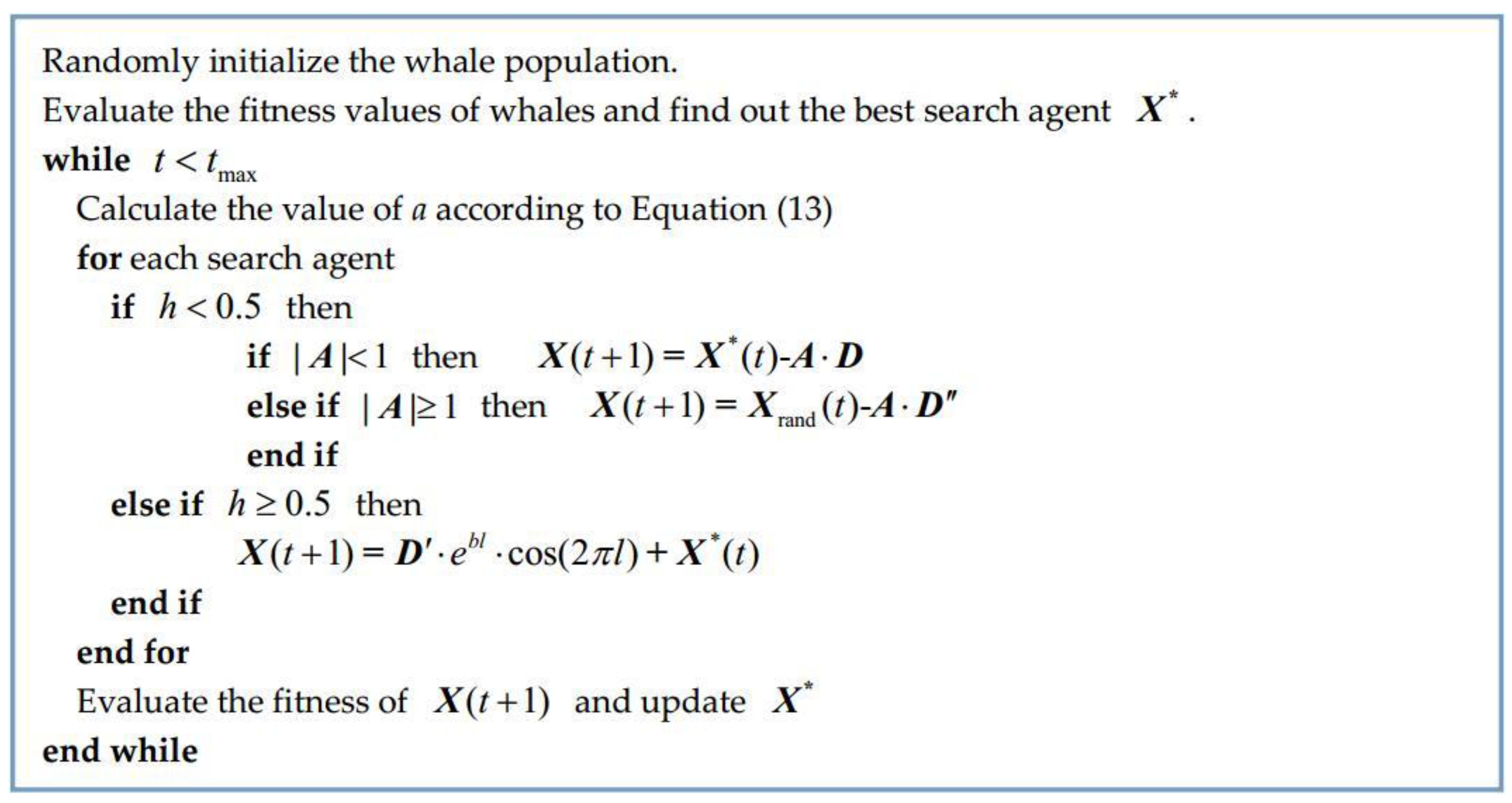
3.3. Pseudo Code of WOA

The pseudo code of the original WOA algorithm can be shown in Figure 1.

4. Implement of the Proposed IWOA

4.1. Scheduling Solution Representation

As mentioned above, the energy-efficient job shop scheduling problem consists of two sub-problems, that is, operation permutation and speed-level selection. To obtain a feasible scheduling scheme, it needs to choose suitable processing speeds for jobs and arrange them on each machine. Therefore, the scheduling solution can be represented by a two-segment string with the size of $2mn$. The first segment tries to arrange the processing sequence of operations on each machine, and the second aims to choose an appropriate speed level for each job.

Taking a $3\times 2$ (three jobs, two machines) EJSP, for example, five speed levels are considered for each job on machines. The scheduling solution can be shown by Figure 2. For the first segment, each element means the job code, where the elements with the same values represent different operations of the same job. For the second segment, each element represents the speed-level selected for the relevant job, which is stored in a given order. $O_{ik}$ represents the $k$th operation of job $i$.

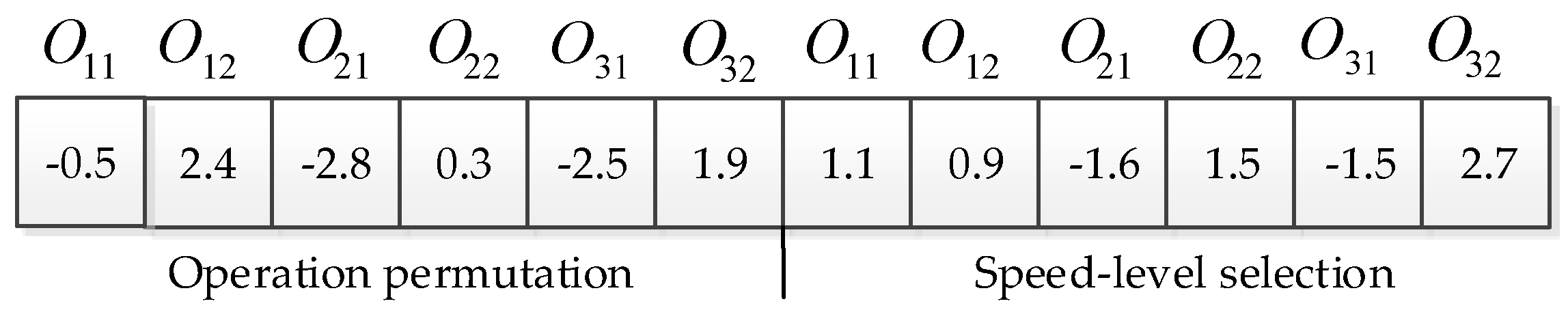
4.2. Individual Position Vector

In the proposed IWOA, the individual position is still a multi-dimensional real vector, which is also made up by two segments, that is, $\mathit{X}=\left\{x(1),x(2),\dots ,x(mn),x(mn+1),\dots ,x(2mn)\right\}$, where $x(j)\in [x_{\min },x_{\max }],j=1,2,\dots ,2mn$. The first segment ${\mathit{X}}_{{}^1}=\left\{x(1),x(2),\dots ,x(mn)\right\}$ presents the information of operation permutation, and the second segment ${\mathit{X}}_{{}^2}=\left\{x(mn+1),\dots ,x(2mn)\right\}$ gives the information of speed-level selection. For the above $3\times 2$ EJSP (three jobs, two machines), the individual position vector can be shown by Figure 3, where element values are stored according to the given order.

4.3. Conversion between Individual Position Vector and Scheduling Solution

The original WOA was proposed to deal with the continuous optimization problem. However, considering the discrete characteristics of the EJSP, it is very important to find a method to establish the mapping relationship between the individual position vector and the discrete scheduling solution. In the previous study, a method is proposed to implement the conversion between the continuous individual vector and the discrete scheduling solution for the classical flexible job shop (FJSP) [39]. It is known that FJSP is made up by operation permutation and machine selection. Seen from Figure 2, the structure of the solution is similar to that of the FJSP, where the speed-level selection is taken place of the machine selection vector. Therefore, the conversion method in the literature [39] is modified for the EJSP in this study. To facilitate the expression, the intervals $[x_{\min },x_{\max }]$ are all set as $[-\epsilon ,\epsilon ],\epsilon >0$ in the proposed method.

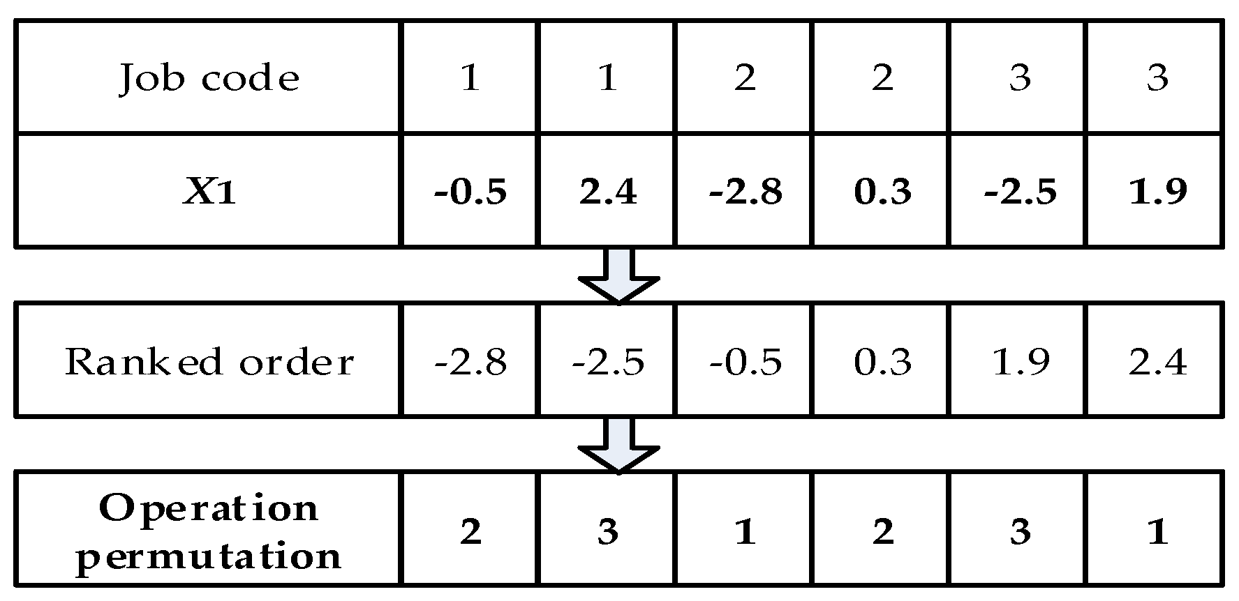
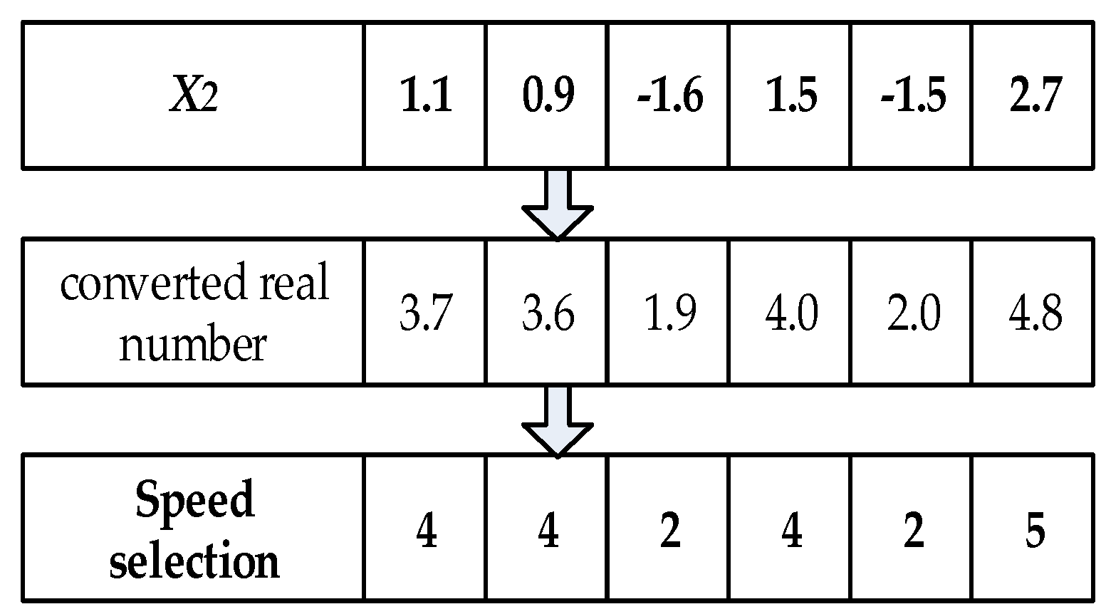
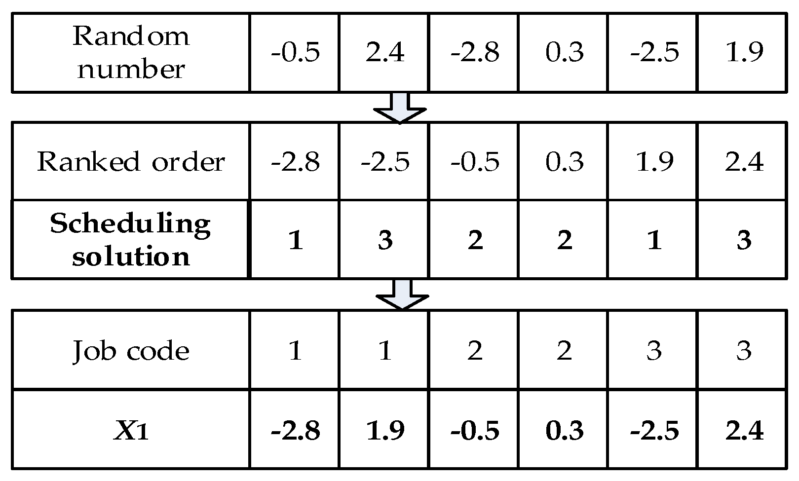
4.3.1. Conversion from Individual Position Vector to Scheduling Solution

For the operation permutation segment, the ranked-order-value (ROV) rule is used to implement the conversion from the individual position to the scheduling solution. In the rule, position values in ${\mathit{X}}_{{}^1}$ are first ranked in an increasing order, then the operation permutation can be acquired according to the new order, which is shown in Figure 4.

For the speed-level selection segment, the conversion process can be modified from the method proposed by Yuan and Xu [40], which can be represented by Equation (19). $z(j)$ denotes the size of alternative speed-level set for the operation corresponding to the jth element, $u(j)$ means the selected speed level, $u(j)\in [1,z(j)]$. In the procedure, $x(j)$ is first converted to a real number belonging to $[1,z(j)]$, then $u(j)$ is given the nearest integer value for the converted real number. For the above example, $\epsilon =3$ and $z(j)=5$. The conversion process is shown in Figure 5.

$$u(j)=round(\frac{x(j)+\epsilon }{2\epsilon }(z(j)-1)+1),1\le j\le mn$$

(19)

4.3.2. Conversion from Scheduling Solution to Individual Position Vector

For the operation permutation segment, $mn$ real numbers are first randomly generated between $[-\epsilon ,\epsilon ]$ and then ranked in an increasing order. According to the ranked order and the scheduling solution, the individual position vector $X_{{}^1}$ can be obtained according to the conversion process in Figure 6.

For the speed-level selection segment, the conversion is generally an inverse process of Equation (19). However, there is a special case, that is, $z(j)=1$, $x(j)$ is obtained by choosing a random value between $[-\epsilon ,\epsilon ]$. The conversion process is shown in Figure 7.

$$x(j)=\{\begin{array}{ll}\frac{2\epsilon }{z(j)-1}(u(j)-1)-\epsilon ,& z(j)\ne 1\\ x(j)\in [-\epsilon ,\epsilon ],& z(j)=1\end{array}$$

(20)

4.4. Initial Scheduling Generation

For a population-based optimization algorithm, the quality of initial solutions is very important for the computational performance. According to the characteristics of the scheduling solution, the population initialization process can be divided into two phases. In the speed-level selection phase, a random generation rule is employed to obtain the initial speeds for jobs. In the operation permutation phase, five dispatching rules are adopted as follows: the Most Work Remaining (MWR), the Most Operation Remaining (MOR), the Shortest Processing Time (SPT), the Longest Processing Time (LPT), and the Random Rule (RR). Each dispatching rule is randomly selected to generate a scheduling solution.

• MWR: give the highest priority to the job with the most amount of remaining work.
• MOR: give the highest priority to the job with the most number of remaining operations.
• SPT: give the highest priority to the job with the shortest processing time.
• LPT: give the highest priority to the job with the longest processing time.
• RR: select jobs for the permutation at random.

4.5. Nonlinear Convergence Factor

Like other population-based optimization algorithms, the cooperation between the abilities of exploitation and exploration is crucial for the performance of the algorithm. As seen from Figure 1, a suitable adjustment of search vector $\mathit{A}$ can allow the WOA algorithm to smoothly transition between exploration and exploitation. By decreasing the value of $\mathit{A}$, some iterations are focused on exploration ($\left|\mathit{A}\right|\ge 1$) and the others are devoted to exploitation ($\left|\mathit{A}\right|<1$). According to Equation (11), the value of $\mathit{A}$ is determined by the variation of $\mathit{a}$. However, $\mathit{a}$ are linearly decreased from 2 to 0 over the course of iterations, which can not well reflect the nonlinear search process of the algorithm. Therefore, a nonlinear adjustment curve of $\mathit{a}$ is adopted in (21), where $a_{\max }$ and $a_{\min }$ define the maximum and minimum values of $a$, respectively.

$$a=a_{\max }-(a_{\max }-a_{\min })\sin (t\pi /(2t_{\max }))$$

(21)

4.6. Mutation Operation

According to the characteristics of the WOA, whales cluster around the local optimum at the latter stage of the optimization, which will decrease the population diversity and lead to premature convergence. In this study, a kind of adaptive mutation operator is presented to overcome this drawback, where the mutation rate of each individual can be calculate according to Equation (15). $p_g$ defines the mutation rate of the gth individual and $f$ represents the fitness function $\raisebox{1ex}{$Q$}\!\left/ \!\raisebox{-1ex}{$F$}\right.$, where Q is a constant. $f_{\max }$ and $f_{\min }$ are the maximum and minimum values of $f$ in the current generation, respectively. In Equation (15), the mutation rate of each whale is changed along with the fitness in the evolution process. If a random number is smaller than $p_g$, the mutation operations for the two segments are conducted.

For the operation permutation segment, an inverse mutation operator is used to inverse the order of elements between two randomly selected positions in a candidate individual. For the speed-level selection segment, a single-point mutation is employed to select a new speed level to take place of the original one, and then a new individual position is obtained by Equation (20).

$$p_g(t)=1-\frac{f_{\max }(t)-f_g(t)}{f_{\max }(t)-f_{\min }(t)}$$

(22)

4.7. Pseudo Code of IWOA

The pseudo code of the IWOA algorithm can be shown in Figure 8.

5. Computational Results

5.1. Experimental Settings

The implementation of the proposed IWOA algorithm is coded by using Fortran language and run on VMware Workstation with 2GB main memory under WinXP. In this section, 38 instances modified from those of the classical JSP (FT06, FT10, and FT20 in the work of [41] and LA01–LA35 in the work of [42]) are used to validate the efficiency of the IWOA. For each instance, ten independent replications are run by different algorithms. Here, the processing times in the classical JSP are taken as the basic processing times. The speed for processing operations can be selected from $v=\left\{v_1,v_2,v_3,v_4,v_5\right\}=\{1.0,1.2,1.5,2.0,2.5\}$. The energy consumption cost per unit time of machine $k$ can be calculated according to $E_{kd}={\xi }_k\times v_d^2,d=1,2,3,4,5$, where ${\xi }_k$ is randomly generated following a discrete uniform distribution in the literature [2,4]. The stand-by energy consumption cost per unit time of machine $k$ is calculated by $S{E}_k={\xi }_k/4$. In addition, the completion time cost per unit time $\lambda$ is set to be 15.0.

5.2. Effectiveness of the Improvement Strategies

In this paper, three strategies are adopted to improve the performance of the IWOA algorithm, namely, DR, NCF, and MO. In this subsection, the effectiveness of the three strategies are first tested. In

Table 1. Effectiveness analysis of improvement strategy.

Instance	IWOA-R				IWOA-L				IWOA-NMO				IWOA
	Best	Avg	SD	Time	Best	Avg	SD	Time	Best	Avg	SD	Time	Best	Avg	SD	Time
FT06	1364.4	1381.5	13.1	27.0	1374.4	1384.3	6.7	27.0	1383.3	1389.8	6.9	15.9	1370.4	1382.8	6.2	26.9
FT10	31,756.9	32,689.8	652.5	108.2	31,809.4	32,564.2	569.2	109.6	31,720.1	32,394.9	322.9	64.0	31,619.3	32,726.4	649.4	107.8
FT20	35,225.1	35,925.9	337.0	111.5	35,138.0	35,888.1	425.9	113.7	35,005.8	35,525.3	370.1	66.2	34,544.2	35,155.7	376.8	111.4
LA01	18,053.5	18,278.0	164.1	40.8	18,031.3	18,281.8	157.6	39.2	18,033.6	18,408.3	243.7	23.6	18,096.0	18,204.8	88.8	39.0
LA02	17,663.3	17,893.5	131.0	38.5	17,699.8	17,935.7	160.5	38.7	17,911.5	18,253.6	218.7	23.3	17,661.0	17,967.5	157.8	38.2
LA03	15,679.5	15,877.2	142.5	38.5	15,765.6	15,989.5	189.1	38.8	15,873.5	16,153.8	183.0	23.2	15,679.6	15,913.4	219.2	38.7
LA04	16,114.6	16,327.7	119.2	38.0	16,223.0	16,384.8	107.1	40.0	16,129.9	16,467.2	215.8	23.5	16,039.7	16,209.3	136.1	38.0
LA05	14,506.1	14,667.6	96.0	38.6	14,447.2	14,657.9	133.4	39.7	14,613.5	14,813.4	138.4	23.6	14,442.6	14,608.0	97.8	38.2
LA06	25,145.6	25,529.1	206.2	68.7	25,248.1	25,654.4	204.1	69.4	25,464.8	25,758.7	196.6	40.8	25,198.4	25,501.0	134.8	68.2
LA07	24,510.7	24,770.1	183.8	67.0	24,534.1	24,868.4	227.2	67.1	24,513.2	24,867.2	238.4	39.9	24,172.9	24,619.2	203.1	66.3
LA08	24,511.2	24,765.4	213.7	73.6	24,717.8	24,889.7	132.6	73.9	24,700.3	24,922.0	140.0	39.5	24,422.8	24,775.7	202.1	67.6
LA09	27,349.1	27,538.6	136.5	72.3	27,401.1	27,692.2	122.0	74.0	27,610.5	27,798.6	149.9	44.0	27,329.5	27,608.6	122.5	73.5
LA10	24,959.0	25,349.7	216.4	73.6	25,210.1	25,455.5	164.4	73.5	25,206.4	25,405.9	164.9	43.9	25,081.3	25,315.5	178.9	73.2
LA11	34,287.2	34,668.2	213.6	112.6	34,406.6	34,697.8	220.4	113.9	34,227.4	34,706.6	233.3	64.6	34,221.7	34,659.8	258.5	110.1
LA12	29,927.1	30,282.2	178.2	110.8	30,213.3	30,432.0	163.0	111.9	30,088.7	30,287.8	159.4	64.3	29,905.6	30,221.5	173.9	111.6
LA13	32,974.4	33,316.7	232.8	110.4	33,379.4	33,617.1	143.1	117.0	33,192.5	33,401.8	124.9	67.5	33,198.1	33,490.7	216.0	110.2
LA14	33,991.7	34,116.7	114.7	113.3	34,084.4	34,478.8	187.5	114.7	33,979.4	34,398.0	249.7	67.2	33,794.5	34,214.3	242.8	114.0
LA15	35,817.5	36,102.2	159.3	113.9	36,017.9	36,327.0	209.0	115.1	35,979.6	36,315.0	258.1	66.2	35,802.4	36,199.8	203.0	113.1
LA16	31,572.7	32,171.2	549.2	109.1	31,746.8	32,480.8	453.5	111.4	32,215.1	32,856.2	313.0	64.5	31,516.7	32,118.2	397.7	108.9
LA17	27,734.0	28,259.8	249.5	110.7	28,258.8	28,710.7	265.3	111.4	28,103.6	28,570.6	277.9	64.4	27,606.6	28,166.0	377.8	110.1
LA18	30,631.3	31,300.5	291.1	106.2	31,147.3	31,530.1	188.4	108.3	31,192.0	31,465.4	243.4	63.0	30,826.6	31,480.9	525.1	107.5
LA19	30,938.3	31,432.7	270.4	108.1	30,951.9	31,608.5	343.4	109.3	30,626.6	31,684.9	491.6	63.3	31,167.9	31,653.8	352.9	108.5
LA20	32,959.8	33,481.9	379.0	108.3	33,121.5	33,816.8	501.0	108.0	33,213.6	33,863.7	365.5	61.6	32,675.2	33,359.4	384.3	104.1
LA21	46,010.4	46,775.4	473.7	199.4	46,475.3	47,252.7	665.3	196.7	45,814.5	46,567.8	707.6	115.4	46,139.7	46,595.8	256.6	190.7
LA22	41,008.2	42,285.9	721.5	191.3	41,528.4	42,418.6	430.6	197.2	40,960.6	42,078.4	640.5	116.3	41,378.6	42,185.1	556.5	193.9
LA23	44,957.1	45,687.4	619.0	191.6	45,303.6	46,203.4	602.4	203.2	45,527.4	46,142.1	722.9	116.1	44,848.3	45,655.5	626.4	195.5
LA24	42,921.1	44,018.8	442.6	191.0	43,142.3	44,258.3	614.3	185.4	42,587.5	43,819.4	775.2	108.0	41,747.3	43,487.9	869.3	191.3
LA25	42,397.1	42,925.9	332.0	184.0	42,805.1	43,693.6	470.3	186.2	42,602.1	43,175.7	310.0	106.4	43,328.0	43,686.9	364.9	185.7
LA26	59,010.9	59,783.1	426.7	289.8	60,087.4	60,912.2	569.9	299.8	58,381.8	59,645.3	745.5	171.7	58,956.5	60,361.9	792.4	292.0
LA27	60,258.6	62,040.3	1017.7	288.8	60,815.2	62,214.4	871.5	286.9	60,106.7	61,706.2	867.3	166.3	60,345.2	61,834.3	701.7	287.3
LA28	59,776.6	60,419.2	606.8	268.6	59,157.5	61,859.0	1448.4	292.5	59,131.6	60,600.6	777.6	162.5	59,361.1	60,933.3	580.5	282.0
LA29	57,139.0	58,076.0	596.4	278.2	56,908.8	58,345.2	1148.2	290.1	56,927.2	58,145.1	705.9	169.8	56,971.4	58,028.9	934.3	289.8
LA30	60,689.9	61,396.5	696.2	279.7	61,680.8	62,924.5	1226.9	280.1	60,856.4	62,305.2	1064.5	156.9	60,849.4	61,970.9	753.8	280.0
LA31	85,498.9	87,045.9	1149.1	532.6	85,708.0	87,871.1	1597.1	587.8	85,180.3	86,549.2	1422.7	320.8	85,121.3	86,301.1	551.2	588.0
LA32	90,282.2	93,019.1	1049.8	572.0	92,704.6	94,834.7	1647.9	572.5	89,949.9	92,833.3	1937.3	321.6	91,552.0	92,848.3	1208.2	570.5
LA33	83,128.1	84,780.9	1376.6	592.1	85,535.2	86,504.5	712.2	563.3	83,408.3	84,776.2	1063.2	314.6	83,406.5	84,898.0	667.4	557.6
LA34	85,278.7	87,079.6	1172.8	596.9	86,813.6	88,850.1	1395.4	590.0	84,950.7	86,471.5	1615.4	334.5	85,921.4	87,369.6	1379.5	578.7
LA35	86,418.3	88,466.7	1606.2	578.2	88,908.5	90,462.3	1168.2	582.1	87,212.1	87,976.7	590.0	327.6	87,327.1	89,208.7	1336.9	563.3

, instance names are listed in the first column, and computational data are reported in the following columns. ‘IWOA’ is the proposed algorithm in this study. ‘IWOA-R’ represents the algorithm where the initial solutions are only created by the random rule. ‘IWOA-L’ represents the algorithm where the elements of $a$ are linearly decreased by Equation (13). ‘IWOA-NMO’ represents the algorithm where the mutation operation is excluded from the IWOA algorithm. In addition, ‘Best’ represents the best value in the ten runs. ‘Avg’ means the average results of the ten runs. ‘SD’ is the standard deviation of total cost obtained by ten runs. ‘Time’ is the average computational time (in seconds) in the ten runs. Boldface denotes the optimal values obtained by algorithms. To facilitate the comparison, the same parameters are set for the compared algorithms, for example, population size is 200 and maximum iteration is 2000.

From the experimental data in Table 1, the following can be observed: (1) In comparisons of the ‘Best’ value, the IWOA algorithm yields 18 optimal values, which is significantly better than the other three algorithms. The second best algorithm, namely IWOA-R, only obtains 10 optimal values. (2) In comparisons of the ‘Avg’ value, the IWOA algorithm yields 16 optimal values, which is more than those of the other three algorithms. The second best algorithm, namely IWOA-R, can obtain 13 optimal values. (3) In comparisons of the ‘SD’ value, IWOA-R performs better than other three algorithms. The second best algorithm, the proposed IWOA algorithm, yields 8 optimal values, which is more than those of IWOA-L and IWOA-NMO. (4) In comparisons of the ‘Time’ value, IWOA-NMO spends a shorter time than other three algorithms. Compared with the IWOA-NMO, the increase of computation time is mainly the result of the addition of the mutation operation in IWOA.

5.3. Effectiveness of the Proposed IWOA

To demonstrate the effectiveness of the proposed IWOA algorithm, the proposed algorithm is compared with genetic algorithm 1 (GA1), genetic algorithm 2 (GA2), and the teaching-learning based optimization (TLBO) algorithm. For GA1, the initial population is generated by the proposed DR. The precedence preserving order-based crossover (POX) and the two-point crossover (TPX) are adopted as the crossover operators for the operation permutation and the speed selection, respectively. In addition, the swap mutation and one-point mutation are adopted for the operation permutation and the speed selection, respectively. For GA2, the algorithm in the work of [18] is used for solving the problem under study. For the TLBO, the algorithm in the work of [43] is modified with the addition of speed selection. Parameters are set as follows: In GA1 and GA2, the population size is 200, the maximum of iteration is 2000, the crossover rate is 0.8, and the mutation rate is 0.1. In the TLBO, the population size is 200 and the maximum of iteration is 2000. Ten independent replications are conducted for each instance.

From the experimental data in

Table 2. Comparison between different algorithms.

Instancce	GA1				GA2				TLBO				IWOA
	Best	Avg	SD	Time	Best	Avg	SD	Time	Best	Avg	SD	Time	Best	Avg	SD	Time
FT06	1528.0	1540.6	10.0	6.2	1550.6	1582.9	20.0	7.3	1639.3	1658.4	13.5	81.9	1370.4	1382.8	6.2	26.9
FT10	37,145.2	38,322.0	819.8	22.8	38,638.7	39,772.5	620.2	30.1	38,719.6	39,618.0	423.7	370.4	31,619.3	32,726.4	649.4	107.8
FT20	41,573.8	42,212.4	496.4	25.7	42,777.3	43,877.3	514.1	32.7	41,716.3	42,161.3	245.1	772.6	34,544.2	35,155.7	376.8	111.4
LA01	20,929.0	21,239.9	166.4	9.9	21,845.8	22,302.7	279.7	11.6	22,766.9	23,052.0	181.5	163.8	18,096.0	18,204.8	88.8	39.0
LA02	20,321.9	20,801.4	219.9	9.8	21,223.0	21,626.4	330.1	11.3	21,480.3	21,875.7	200.7	164.8	17,661.0	17,967.5	157.8	38.2
LA03	18,436.8	18,895.8	299.5	9.9	19,269.9	19,624.5	227.7	11.5	19,640.7	20,034.8	158.8	163.2	15,679.6	15,913.4	219.2	38.7
LA04	18,390.9	19,037.8	277.2	9.9	19,085.3	19,620.1	216.7	11.5	19,983.2	20,447.2	265.1	163.1	16,039.7	16,209.3	136.1	38.0
LA05	16,501.3	16,829.2	185.7	9.8	17,424.2	17,732.9	228.1	11.6	18,111.9	18,372.4	121.5	163.4	14,442.6	14,608.0	97.8	38.2
LA06	29,645.5	29,832.5	156.9	16.7	30,332.6	31,156.2	428.6	21.1	30,925.3	31,757.5	351.9	390.8	25,198.4	25,501.0	134.8	68.2
LA07	28,288.9	28,821.7	306.8	16.7	29,614.2	30,278.9	422.5	21.2	30,293.6	30,494.5	156.5	409.5	24,172.9	24,619.2	203.1	66.3
LA08	28,418.7	28,959.5	288.3	17.0	29,442.4	30,591.2	463.1	21.3	30,574.5	30,829.1	168.8	416.2	24,422.8	24,775.7	202.1	67.6
LA09	31,487.4	32,028.0	300.4	16.9	32,652.8	33,383.0	476.8	21.3	33,563.3	34,137.6	391.2	412.3	27,329.5	27,608.6	122.5	73.5
LA10	29,021.5	29,703.9	356.9	16.8	30,753.2	31,272.7	276.3	21.2	32,018.4	32,311.7	201.3	416.1	25,081.3	25,315.5	178.9	73.2
LA11	39,735.1	40,732.2	563.2	25.6	40,691.1	42,380.5	694.1	29.9	42,098.2	42,568.8	250.3	831.8	342,21.7	34,659.8	258.5	110.1
LA12	34,360.3	35,109.6	567.1	25.2	36,116.2	36,705.9	364.6	30.2	36,685.3	37,024.0	210.6	767.1	29,905.6	30,221.5	173.9	111.6
LA13	37,641.6	38,759.5	902.9	25.5	40,046.0	41,036.5	377.0	30.8	40,866.4	41,199.9	168.7	775.3	33,198.1	33,490.7	216.0	110.2
LA14	40,079.5	40,657.0	407.2	25.5	42,035.5	42,668.4	307.0	30.3	42,644.1	43,063.7	235.5	804.6	33,794.5	34,214.3	242.8	114.0
LA15	42,138.3	42,630.5	355.8	25.6	44,265.0	44,865.7	406.6	30.6	43,729.4	44,087.5	250.3	800.1	35,802.4	36,199.8	203.0	113.1
LA16	37,245.6	38,160.1	775.0	23.2	39,352.3	40,191.7	505.5	28.0	39,637.1	40,341.5	366.2	406.5	31,516.7	32,118.2	397.7	108.9
LA17	32,693.6	33,180.5	450.0	23.0	34,319.1	35,011.7	475.3	27.9	34,707.3	35,280.3	375.9	400.3	27,606.6	28,166.0	377.8	110.1
LA18	35,469.3	36,751.3	648.4	23.2	37,326.8	38,536.1	611.9	27.9	38,204.9	39,038.9	368.0	392.1	30,826.6	31,480.9	525.1	107.5
LA19	36,099.4	37,003.0	649.9	23.1	38,359.7	39,177.2	405.7	27.7	38,186.7	38,962.7	391.6	404.3	31,167.9	31,653.8	352.9	108.5
LA20	38,179.1	39,348.4	546.1	22.8	40,626.2	41,834.9	596.4	28.1	41,519.6	41,982.8	278.8	400.4	32,675.2	33,359.4	384.3	104.1
LA21	54,607.7	55,786.4	641.3	40.5	57,276.3	58,907.5	656.6	52.5	56,961.4	57,707.3	389.4	949.1	46,139.7	46,595.8	256.6	190.7
LA22	49,559.5	51,284.0	755.0	40.6	51,457.2	53,373.3	924.2	50.9	52,280.6	52,541.4	183.0	893.2	41,378.6	42,185.1	556.5	193.9
LA23	53,917.7	54,612.9	561.0	40.6	56,499.0	57,683.4	682.8	52.0	56,709.3	57,164.8	259.8	955.8	44,848.3	45,655.5	626.4	195.5
LA24	51,056.0	52,393.9	826.4	40.7	54,503.0	55,457.0	716.7	53.2	53,032.8	54,086.9	559.4	936.2	41,747.3	43,487.9	869.3	191.3
LA25	51,583.8	52,236.1	389.8	40.5	54,128.9	51,823.4	496.6	51.8	52,744.1	53,644.7	485.7	940.4	43,328.0	43,686.9	364.9	185.7
LA26	70,951.3	72,097.3	895.9	60.7	75,180.8	75,817.0	547.6	80.9	73,634.3	73,967.6	288.3	1807.0	58,956.5	60,361.9	792.4	292.0
LA27	72,413.8	74,974.8	1004.8	61.3	76,673.0	78,085.6	807.9	86.4	75,245.7	75,683.7	322.5	1845.4	60,345.2	61,834.3	701.7	287.3
LA28	71,365.7	72,774.3	782.7	61.3	74,918.6	76,472.9	834.1	85.3	73,722.1	74,669.0	608.7	1780.7	59,361.1	60,933.3	580.5	282.0
LA29	67,354.4	69,077.6	1235.2	60.9	70,744.8	72,150.4	1041.7	84.8	69,980.3	70,706.9	482.7	1777.3	56,971.4	58,028.9	934.3	289.8
LA30	72,707.5	73,966.6	589.3	59.8	76,737.0	77,547.9	659.0	85.1	74,160.6	75,329.5	711.6	1792.8	60,849.4	61,970.9	753.8	280.0
LA31	99,556.7	104,319.6	2041.1	113.8	106,691.4	108,275.1	979.2	168.9	103,707.5	104,566.3	703.8	4807.2	85,121.3	86,301.1	551.2	588.0
LA32	110,241.3	112,299.6	1208.0	113.8	115,254.6	117,103.4	859.6	165.9	113,250.8	113,450.3	220.1	4958.3	91,552.0	92,848.3	1208.2	570.5
LA33	100,960.7	102,467.9	1171.0	111.3	104,826.8	106,660.0	957.1	172.8	102,476.4	103,051.6	428.6	5273.3	83,406.5	84,898.0	667.4	557.6
LA34	102,234.6	104,521.0	1902.4	111.2	106,811.5	108,573.6	734.5	172.7	105,440.0	105,768.8	275.5	5064.8	85,921.4	87,369.6	1379.5	578.7
LA35	104,497.8	105,599.2	1097.5	112.0	107,670.7	110,468.2	1210.6	190.6	106,133.5	106,803.1	720.4	4814.7	87,327.1	89,208.7	1336.9	563.3

, the following can be easily observed: (1) In comparisons of the ‘Best’ value, the proposed IWOA algorithm can obtain all the optimal values. (2) In comparisons of the ‘Avg’ value, the proposed IWOA algorithm can also obtain all the optimal values. (3) In comparisons of the ‘SD’ value, the IWOA algorithm yields 15 optimal values, which is better than GA1 and GA2. (4) In comparisons of the ‘Time’ value, GA1 spends a shorter time than other two algorithms. The proposed IWOA spends more time because it contains the conversion process between the individual position vector and the scheduling solution. However, by comparison, the IWOA can yield the best values in an acceptable time.

6. Conclusions

In this study, an improved whale optimization algorithm (IWOA) is proposed to solve an energy-efficient job shop scheduling problem. The conversion method between the scheduling solution and the individual position vector is first designed. After that, three improvement strategies are adopted in the algorithm, namely, the dispatching rules (DR), the nonlinear convergence factor (NCF), and the mutation operation (MO). The DR is adopted to generate the initial solutions. The NCF is used to coordinate the capacity of exploration and exploitation. The MO is employed to avoid the premature convergence.

Extensive experiments are conducted for testing the performance of the IWOA algorithm. From the experimental results, it can be seen that the proposed improvement strategies can improve the computational result of the algorithm. In addition, compared with GA1, GA2, and TLBO, the proposed IWOA algorithm can obtain better results in an acceptable time.

In future work, the energy-efficient scheduling will be further studied by considering some more practical constraints, for example, flexible processing routing, time-of-use electricity policy, and renewable energy, among others. In addition, the energy-efficient scheduling problem will be extended to some complex workshop, such as flexible job shop and assembly job shop, among others.

References

1. Duflou, J.R.; Sutherland, J.W.; Dornfeld, D.; Herrmann, C.; Jeswiet, J.; Kara, S.; Hauschild, M.; Kellens, K. Towards energy and resource efficient manufacturing: A processes and systems approach. CIRP Ann.-Manuf. Technol. 2012, 61, 587–609. [Google Scholar] [CrossRef]
2. Fang, K.; Uhan, N.; Zhao, F.; Sutherland, J.W. A New Shop Scheduling Approach in Support of Sustainable Manufacturing; Glocalized solutions for sustainability in manufacturing; Springer: Berlin/Heidelberg, Germany, 2011; pp. 305–310. [Google Scholar]
3. Liu, Y.; Dong, H.; Lohse, N.; Petrovic, S.; Gindy, V. An investigation into minimising total energy consumption and total weighted tardiness in job shops. J. Clean. Prod. 2014, 65, 87–96. [Google Scholar] [CrossRef]
4. Mouzon, G.; Yildirim, M.B.; Twomey, J. Operational methods for minimization of energy consumption of manufacturing equipment. Int. J. Prod. Res. 2007, 45, 4247–4271. [Google Scholar] [CrossRef] [Green Version]
5. Mouzon, G.; Yildirim, M.B. A framework to minimise total energy consumption and total tardiness on a single machine. Int. J. Sustain. Eng. 2008, 1, 105–116. [Google Scholar] [CrossRef] [Green Version]
6. Yildirim, M.B.; Mouzon, G. Single-machine sustainable production planning to minimize total energy consumption and total completion time using a multiple objective genetic algorithm. IEEE. Trans. Eng. Manag. 2012, 59, 585–597. [Google Scholar] [CrossRef]
7. Shrouf, F.; Ordieres-Meré, J.; García-Sánchez, A.; Ortega-Mier, M. Optimizing the production scheduling of a single machine to minimize total energy consumption costs. J. Clean. Prod. 2014, 67, 197–207. [Google Scholar] [CrossRef]
8. Che, A.; Zeng, Y.; Lyu, K. An efficient greedy insertion heuristic for energy-conscious single machine scheduling problem under time-of-use electricity tariffs. J. Clean. Prod. 2016, 129, 565–577. [Google Scholar] [CrossRef]
9. Li, J.Q.; Sang, H.Y.; Han, Y.Y.; Wang, C.G.; Gao, K.Z. Efficient multi-objective optimization algorithm for hybrid flow shop scheduling problems with setup energy consumptions. J. Clean. Prod. 2018, 181, 584–598. [Google Scholar] [CrossRef]
10. Liu, G.S.; Zhang, B.X.; Yang, H.D.; Chen, X.; Huang, G.Q. A branch-and-bound algorithm for minimizing the energy consumption in the PFS problem. Math. Probl. Eng. 2013, 2013, 546810. [Google Scholar] [CrossRef]
11. Dai, M.; Tang, D.; Giret, A.; Salido, M.A.; Li, W.D. Energy-efficient scheduling for a flexible flow shop using an improved genetic-simulated annealing algorithm. Robot. Comput.-Int. Manuf. 2013, 29, 418–429. [Google Scholar] [CrossRef] [Green Version]
12. Ding, J.Y.; Song, S.; Wu, C. Carbon-efficient scheduling of flow shops by multi-objective optimization. Eur. J. Oper. Res. 2016, 248, 758–771. [Google Scholar] [CrossRef]
13. Mansouri, S.A.; Aktas, E.; Besikci, U. Green scheduling of a two-machine flowshop: Trade-off between makespan and energy consumption. Eur. J. Oper. Res. 2016, 248, 772–788. [Google Scholar] [CrossRef]
14. Luo, H.; Du, B.; Huang, G.Q.; Chen, H.; Li, X. Hybrid flow shop scheduling considering machine electricity consumption cost. Int. J. Prod. Econ. 2013, 146, 423–439. [Google Scholar] [CrossRef]
15. Salido, M.A.; Escamilla, J.; Giret, A.; Barber, F. A genetic algorithm for energy-efficiency in job-shop scheduling. Int. J. Adv. Manuf. Technol. 2016, 85, 1303–1314. [Google Scholar] [CrossRef]
16. Zhang, R.; Chiong, R. Solving the energy-efficient job shop scheduling problem: A multi-objective genetic algorithm with enhanced local search for minimizing the total weighted tardiness and total energy consumption. J. Clean. Prod. 2016, 112, 3361–3375. [Google Scholar] [CrossRef]
17. Tang, D.; Dai, M. Energy-efficient approach to minimizing the energy consumption in an extended job-shop scheduling problem. Chin. J. Mech. Eng. 2015, 28, 1048–1055. [Google Scholar] [CrossRef]
18. Escamilla, J.; Salido, M.A.; Giret, A.; Barber, F. A metaheuristic technique for energy-efficiency in job-shop scheduling. Knowl. Eng. Rev. 2016, 31, 475–485. [Google Scholar] [CrossRef]
19. Yin, L.; Li, X.; Gao, L.; Lu, C.; Zhang, Z. Energy-efficient job shop scheduling problem with variable spindle speed using a novel multi-objective algorithm. Adv. Mech. Eng. 2017, 9. [Google Scholar] [CrossRef] [Green Version]
20. Wang, G.G.; Tan, Y. Improving metaheuristic algorithms with information feedback models. IEEE. Trans. Cybern. 2017. [Google Scholar] [CrossRef] [PubMed]
21. Wang, G.G.; Gandomi, A.H.; Alavi, A.H. An effective krill herd algorithm with migration operator in biogeography-based optimization. Appl. Math. Model. 2014, 38, 2454–2462. [Google Scholar] [CrossRef]
22. Wang, G.G.; Gandomi, A.H.; Alavi, A.H. Stud krill herd algorithm. Neurocomputing 2014, 128, 363–370. [Google Scholar] [CrossRef]
23. Wang, G.G.; Guo, L.; Gandomi, A.H.; Hao, G.S.; Wang, H. Chaotic krill herd algorithm. Inform. Sci. 2014, 274, 17–34. [Google Scholar] [CrossRef]
24. Wang, G.; Guo, L.; Wang, H.; Duan, H.; Liu, L.; Li, J. Incorporating mutation scheme into krill herd algorithm for global numerical optimization. Neural Comput. Appl. 2014, 24, 853–871. [Google Scholar] [CrossRef]
25. Feng, Y.; Wang, G.G.; Dong, J.; Wang, L. Opposition-based learning monarch butterfly optimization with Gaussian perturbation for large-scale 0-1 knapsack problem. Comput. Electr. Eng. 2018, 67, 454–468. [Google Scholar] [CrossRef]
26. Rizk-Allah, R.M.; El-Sehiemy, R.A.; Wang, G.G. A novel parallel hurricane optimization algorithm for secure emission/economic load dispatch solution. Appl. Soft. Comput. 2018, 63, 206–222. [Google Scholar] [CrossRef]
27. Jiang, T.H.; Zhang, C. Application of Grey Wolf Optimization for solving combinatorial problems: Job shop and flexible job shop scheduling cases. IEEE. Access. 2018, 6, 26231–26240. [Google Scholar] [CrossRef]
28. Jiang, T.H.; Deng, G.L. Optimizing the low-carbon flexible job shop scheduling problem considering energy consumption. IEEE. Access. 2018, 6, 46346–46355. [Google Scholar] [CrossRef]
29. Han, Y.Y.; Gong, D.W.; Jin, Y.C.; Pan, Q.K. Evolutionary Multi-objective Blocking Lot-streaming Flow Shop Scheduling with Machine Breakdowns. IEEE. Trans. Cybern. 2018. [Google Scholar] [CrossRef]
30. Han, Y.Y.; Liang, J.; Pan, Q.K.; Li, J.Q. Effective hybrid discrete artificial bee colony algorithms for the total flow time minimization in the blocking flow shop problem. Int. J. Adv. Manuf. Technol. 2013, 67, 397–414. [Google Scholar] [CrossRef]
31. Han, Y.Y.; Pan, Q.K.; Li, J.Q.; Sang, H.Y. An improved artificial bee colony algorithm for the blocking flow shop scheduling problem. Int. J. Adv. Manuf. Technol. 2012, 60, 1149–1159. [Google Scholar] [CrossRef]
32. Li, J.Q.; Duan, P.Y.; Sang, H.Y.; Wang, S.; Liu, Z.M.; Duan, P. An efficient optimization algorithm for resource-constrained steelmaking scheduling problems. IEEE. Access. 2018, 6, 33883–33894. [Google Scholar] [CrossRef]
33. Mirjalili, S.; Lewis, A. The whale optimization algorithm. Adv. Eng. Softw. 2016, 95, 51–67. [Google Scholar] [CrossRef]
34. Ling, Y.; Zhou, Y.; Luo, Q. Lévy flight trajectory-based whale optimization algorithm for global optimization. IEEE. Access. 2017, 5, 6168–6186. [Google Scholar] [CrossRef]
35. Mafarja, M.; Mirjalili, S. Whale optimization approaches for wrapper feature selection. Appl. Soft. Comput. 2018, 62, 441–453. [Google Scholar] [CrossRef]
36. El Aziz, M.A.; Ewees, A.A.; Hassanien, A.E. Multi-objective whale optimization algorithm for content-based image retrieval. Multimed. Tools Appl. 2018, 77, 26135–26172. [Google Scholar] [CrossRef]
37. Abdel-Basset, M.; El-Shahat, D.; Sangaiah, A.K. A modified nature inspired meta-heuristic whale optimization algorithm for solving 0–1 knapsack problem. Int. J. Mach. Learn. Cybern. 2017, 1–20. [Google Scholar] [CrossRef]
38. Abdel-Basset, M.; Manogaran, G.; El-Shahat, D.; Mirjalili, S. A hybrid whale optimization algorithm based on local search strategy for the permutation flow shop scheduling problem. Future Gener. Comput. Syst. 2018, 85, 129–145. [Google Scholar] [CrossRef]
39. Jiang, T.H. Flexible job shop scheduling problem with hybrid grey wolf optimization algorithm. Control Decis. 2018, 33, 503–508. (In Chinese) [Google Scholar]
40. Yuan, Y.; Xu, H. Flexible job shop scheduling using hybrid differential evolution algorithms. Comput. Ind. Eng. 2013, 65, 246–260. [Google Scholar] [CrossRef]
41. Fisher, H.; Thompson, G.L. Probabilistic learning combinations of local job-shop scheduling rules. Ind. Sched. 1963, 3, 225–251. [Google Scholar]
42. Lawrence, S. Resource Constrained Project Scheduling: An Experimental Investigation of Heuristic Scheduling Techniques; Graduate School of Industrial Administration (GSIA), Carnegie Mellon University: Pittsburgh, PA, USA, 1984. [Google Scholar]
43. Baykasoglu, A.; Hamzadayi, A.; Kose, S.Y. Testing the performance of teaching-learning based optimization (TLBO) algorithm on combinatorial problems: Flow shop and job shop scheduling cases. Inform. Sci. 2014, 276, 204–218. [Google Scholar] [CrossRef]
Figure 1. The pseudo code of the original whale optimization algorithm (WOA).
Mathematics 06 00220 g001
Figure 2. Scheduling solution representation.
Mathematics 06 00220 g002
Figure 3. Individual position vector.
Mathematics 06 00220 g003
Figure 4. The conversion process from individual position vector to operation permutation.
Mathematics 06 00220 g004
Figure 5. The conversion process from individual position vector to speed-level selection.
Mathematics 06 00220 g005
Figure 6. The conversion process from operation permutation to individual position vector.
Mathematics 06 00220 g006
Figure 7. The conversion process from speed-level selection to individual position vector.
Mathematics 06 00220 g007
Figure 8. The pseudo code of the improved WOA (IWOA).
Mathematics 06 00220 g008