Morphogenesis of the Zeta Function in the Critical Strip by Computational Approach

Abstract

This article proposes a morphogenesis interpretation of the zeta function by computational approach by relying on numerical approximation formulae between the terms and the partial sums of the series, divergent in the critical strip. The goal is to exhibit structuring properties of the partial sums of the raw series by highlighting their morphogenesis, thanks to the elementary functions constituting the terms of the real and imaginary parts of the series, namely the logarithmic, cosine, sine, and power functions. Two essential indices of these sums appear: the index of no return of the vagrancy and the index of smothering of the function before the resumption of amplification of its divergence when the index tends towards infinity. The method consists of calculating, displaying graphically in 2D and 3D, and correlating, according to the index, the angles, the terms and the partial sums, in three nested domains: the critical strip, the critical line, and the set of non-trivial zeros on this line. Characteristics and approximation formulae are thus identified for the three domains. These formulae make it possible to grasp the morphogenetic foundations of the Riemann hypothesis (RH) and sketch the architecture of a more formal proof.

1. Introduction

1.1. The Historical Stages of the Conjecture

In 1859, Riemann [1] produced the famous Riemann Hypothesis (RH) and demonstrated the functional equation $\forall s\in ℂ, s\ne 0,1 : \zeta \left(s\right)=2^s{\pi }^{s-1}sin\left(\frac{\pi s}{2}\right)\Gamma \left(1-s\right)\zeta \left(1-s\right)$. The book The Theory of the Riemann Zeta-Function by EC Titchmarsh [2] presents a synthesis on the subject with the various advances, notably those of Hadamard [3] and La Vallée Poussin [4] in 1896, and the work of Littlewood [5] in 1912, Hardy [6] in 1914 and Hardy–Littlewood [7] in 1921. There is a countably infinite set of non-trivial zeros $y_{izero}$ of the ζ function on the critical line, $s=½+iy, y\in ℝ$, with an estimation of the average density of zeros on the critical line. The conjecture states that there are no non-trivial zeros outside this critical line. The ζ function of the complex variable $s=x+iy, s\in ℂ, x>1,y\in ℝ \mathrm{such} \mathrm{that} \zeta \left(s\right)={{\displaystyle \sum }}_{n=1}^{\infty }{n}^{-s}$ is continuous, differentiable and of class ${\mathrm{C}}^{\infty }$. Since ${{\displaystyle \sum }}_{n=1}^{\infty }{n}^{-s}$ diverges in the critical strip, we define $\zeta$ in this strip as follows: $\zeta \left(s\right)=\frac{{{\displaystyle \sum }}_{n=1}^{\infty }{\left(-1\right)}^{n-1}{n}^{-s}}{1-2^{-s+1}}$. The complex value $\zeta \left(s\right)=0$, that is $\Re (\zeta \left(s\right))=C\left(x,y\right)=0 \mathrm{and} \Im (\zeta \left(s\right))=S\left(x,y\right)=0$, is a regular value of the function.

Several approaches can be distinguished to apprehend the demonstration of this conjecture.

• The Fourier approach by spectral analysis;

The Fourier series decomposition of the Riemann function is natural, since it is a question of bringing both sums closer together the Fourier series of period T, $f\left(x\right)=a_0+{{\displaystyle \sum }}_{n=1}^{\infty }\left(a_{n}cosn2\pi x/T+b_{n}sinn2\pi x/T\right)$ and the Riemann series $\zeta \left(x+iy\right)={{\displaystyle \sum }}_{n=1}^{\infty }\left(n^{-x}cosylogn-i n^{-x}sinylogn\right)$. The Hilbert–Pólya program assumes that zeros are the eigenvalues of a Hermitian operator or a random Hermitian matrix: the spectral theory, in connection with quantum mechanics and the Hamiltonian of a particle, and in connection with functional analysis, continues this line of research.

• Dirichlet’s L-functions and modular forms;

An L-function is a ζ function with coefficients. The Dirichlet series were introduced by P.G. Lejeune-Dirichlet [8] in 1837 to show the existence of an infinity of prime numbers in arithmetic progressions (of type $a+nq$ with $a \mathrm{and} q$ coprime). They are of the form ${{\displaystyle \sum }}_{n=1}^{\infty }{a}_n{n}^{-s}, a_n\in ℂ$. It is therefore a question of plunging the Riemann function into a larger space since the RH is expressed in terms of zeros of the analytic extension of a sum function of a Dirichlet series. These series form a unitary commutative ring. A Dirichlet character $\mathrm{modulo} m$ is a multiplicative, periodic function of period $m$. A Dirichlet L-function, attached to $\chi$, is a series $L\left(\chi ,s\right)={{\displaystyle \sum }}_{n=1}^{\infty }\chi \left(n\right)/n^s$.

• The conjecture has analogues for varieties on finite fields;

Artin [9] introduced the analog ζ function for finite fields. Hasse [10] demonstrated the RH for curves of genus 1. Weil [11] separated the problem from the algebraic framework and placed it in a geometrical context and Deligne [12] demonstrated the RH in 1973 for the curves of genus $g⩾1$ on a finite field. However, the branch on the finite fields is different from that on the field of the numbers, because the $\zeta$ functions and the ξ functional equations associated are different. The $\zeta$ function is $Z\left(C,t\right)={{\displaystyle \prod }}_{i=1}^{2g}(1-{\alpha }_{i}t)/\left(1-t\right)\left(1-qt\right)$ on Frobenius ${\mathbb{F}}_q$, with $t=q^{-s}$, for a curve $C$ of genus $g$, and the functional equation is $Z\left(C,1/qt\right)=q^{1-g}{t}^{2-2g}Z\left(C,t\right)$. This branch, however, allowed the emergence of algebraic geometry, i.e., to give a geometrical point of view to the Riemann function, which until then had remained a problem of complex analysis and theory of numbers, in Euler’s and Riemann’s vision.

1.2. The Interactive Computational Approach

A computational approach is proposed to illustrate the RH. Abstractions that are not directly operational numerically are dispensed with, and the field of the $ℂ$ complexes and the properties of the holomorphic functions are abandoned. We focus on the real functions of the partial sums of the raw series in the critical strip in order to compute and numerically compare the studied entities. 2D and 3D curves, surfaces and scatter plots are visualized to observe and interpret mathematical phenomena. This long interactive work on thousands of figures makes it possible to exclude bad intuitions, to reveal new relationships, to discover valid laws pertaining to the critical strip and thus to open the outline of a formal demonstration. However, we are constrained by several obstacles:

• Ontological: The calculation does not prove anything, but allows lessons to be learned.
• Methodological: The Riemann $\zeta$ function diverges in the critical strip $𝓢$. This obstacle is usually solved by the powerful arsenal of holomorphic functions. We are led to consider the analytic extension by the Dirichlet η function, which converges in this strip $𝓢$. This obstacle is circumvented by considering only partial sums, since it is interesting to analyze the numerical values and the behavior of the partial sums of the divergent series in Borel’s vision [13], according to the indices and the terms which compose them.
• Technical: The functional equation $\zeta \left(s\right)=\xi \left(s\right).\zeta \left(1-s\right) \mathrm{with} \xi \left(s\right)={\pi }^{\left(s-½\right)}\frac{\Gamma \left(\left(1-s\right)/2\right)}{\Gamma \left(s/2\right)}$ is a function which implements the Euler’s complex Gamma function $\Gamma \left(s\right)={{\displaystyle \int }}_0^{\infty }{e}^{-t}{t}^{s-1}dt$, which takes numerical values which are difficult to express in a floating point representation. A 64-bit computer only considers positive rational numbers ranging from $4.94\times {10}^{-324}$ to $1.8\times {10}^{308}$, whereas, for example, $\Gamma \left(½+i 475\right)=\left(-1.22+i 1.94\right){10}^{-324}$ but $\Gamma \left(½+i {10}^5\right)=\left(-3+2i\right){10}^{-68219}$. Computer libraries like mpmath [14] are used to deal with these difficulties.

1.3. Structure of the Article

After the introduction, Section 2 presents the data used, as well as the mathematical and computational methods and tools, the theoretical difficulties, the related work and ends with a metaphor of the conjecture. Section 3 gives the results of the study with graphical representations in 2D and 3D. After an observation of the surfaces and curves relating to the ζ function and the partial sums, we propose anamorphoses to visualize the curves and the scatter plots; we study the anatomy of the components and the morphology of the partial sums, to generate approximation formulae. Section 4 discusses the results, explains the morphogenesis, shows the comparison with the Euler–Maclaurin formula, sketches the architecture of a demonstration, and proposes links with signal theory, shows the links with the Fresnel integrals, gives an interpretation of the conjecture by a conflict of homotheties and offers insights before the conclusion.

2. Materials and Methods

2.1. Notations

We denote $s=x+i y=r e^{i\alpha }; s∊ℂ; x, y, r∊ℝ; \alpha ∊\left[0,2\pi \right]$ Throughout the article, we assume $0\le x\le 1, y>0, r\ge 0$. The Riemann $\zeta$ function is written as

$$\zeta \left(s\right)=\zeta \left(x+i y\right)={{\displaystyle \sum }}_{n=1}^{\infty }{n}^{-s}=C-i S={{\displaystyle \sum }}_{n=1}^{\infty }(cos{\alpha }_n-i sin{\alpha }_n)/n^x; {\alpha }_n=y log\left(n\right) mod 2\pi .$$

In the critical strip, the Riemann $\zeta$ function is written as

$$\zeta \left(s\right)=\frac{{{\displaystyle \sum }}_{n=1}^{\infty }{\left(-1\right)}^{n-1}{n}^{-s}}{1-2^{-s+1}}=C-i S=\frac{{{\displaystyle \sum }}_{n=1}^{\infty }{\left(-1\right)}^{n-1}(cos{\alpha }_n-i sin{\alpha }_n)/n^x}{1-2^{-s+1}}.$$

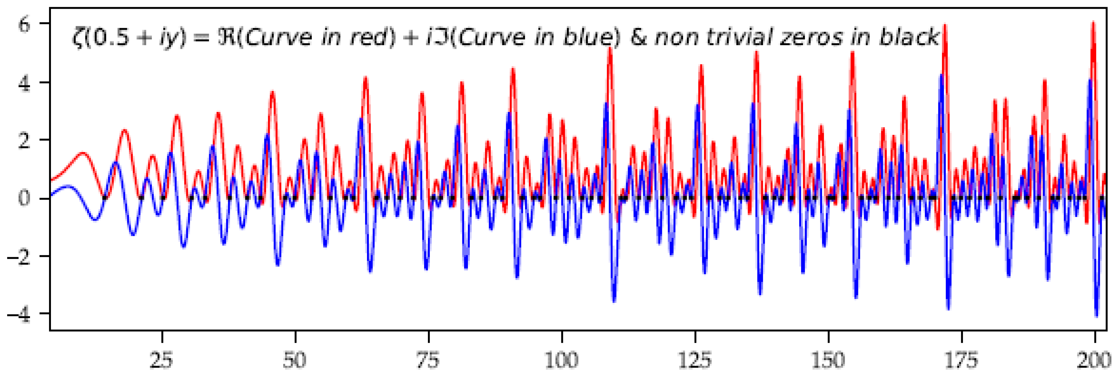
$C \mathrm{and} S$ are two real functions of two real variables $\left(x, y\right)$. RH asserts that the iso-value 0 of the two surfaces $C \mathrm{and} S$ intersects exclusively on the line $x=½$, in a number of values $y_{izero}$ (${\aleph }_0$ values, according to Hardy’s theorem), called non-trivial zeros.

The $\zeta$ function extends meromorphically to the domain $x\ge 0$, with a simple pole in $s=1$ of residue 1. In the critical strip, the Dirichlet series is: $\eta \left(s\right)={{\displaystyle \sum }}_{k=1}^{\infty }{\left(-1\right)}^{k-1}{k}^{-s}=\left(1-2^{s-1}\right)\zeta \left(s\right)$.

We consider the three nested sets $𝓢, 𝓛, 𝓩$:

• Critical strip: $𝓢:=\left\{s\in ℂ : x\in \left[0,1\right]\right\}$
• Critical line: $𝓛:=\left\{s\in ℂ : x=½\right\}$
• Non-trivial zeros: $𝓩:=\left\{s_{izero}=½+i{y}_{izero};\zeta \left(s_{izero}\right)=\eta \left(s_{izero}\right)=0\right\}$.

We call $ℨ$ the set of non-trivial zeros without the constraint of being on the critical line $𝓛:$ $ℨ:=\{s_{izero}=x+iy\in ℂ\}$.

Throughout the study, the partial sums in the critical strip $𝓢$ are used:

• ${\sigma }_n\left(s\right)={{\displaystyle \sum }}_{k=1}^n{z}_k={{\displaystyle \sum }}_{k=1}^n{k}^{-s}=\Re \left[{\sigma }_n\left(s\right)\right]+i \Im \left[{\sigma }_n\left(s\right)\right]$; $\zeta \left(s\right)=\Re \left[\zeta \left(s\right)\right]+i \Im \left[\zeta \left(s\right)\right]$;
• $C_n\left(x,y\right)={{\displaystyle \sum }}_{k=1}^{n}cos\left[ylog\left(k\right)modulo 2\pi \right]/k^x$; $C\left(x,y\right)=\Re \left[\zeta \left(s\right)\right]$;
• $S_n\left(x,y\right)={{\displaystyle \sum }}_{k=1}^{n}sin\left[ylog\left(k\right)modulo 2\pi \right]/k^x$; $S\left(x,y\right)=-\Im \left[\zeta \left(s\right)\right]$;

In the following, we use Euler’s complex Gamma function extended meromorphically to the whole complex plane $\Gamma \left(z\right)={{\displaystyle \int }}_0^{\infty }{t}^{z-1}{e}^{-t}dt$, with complement formula $\Gamma \left(s\right)\Gamma \left(1-s\right)=\pi /sin\left(\pi s\right)$ and distribution formula $\Gamma \left(z\right)\Gamma \left(z+½\right)=2^{1-2z}\sqrt{\pi } \Gamma \left(z\right)$.

We use the Taylor series: $f\left(z\right)={{\displaystyle \sum }}_{n=0}^{\infty }\frac{f^{\left(n\right)}\left(a\right)}{n!}{\left(z-a\right)}^n$.

We also use the Fresnel functions

$$C_F\left(x\right)={{\displaystyle \int }}_0^{x}cos\left(t^2\right)dt={{\displaystyle \sum }}_{n=0}^{\infty }\frac{{\left(-1\right)}^n{x}^{4n+1}}{\left(2n\right)!\left(4n+1\right)}.$$

and

$$S_F\left(x\right)={{\displaystyle \int }}_0^{x}sin\left(t^2\right)dt={{\displaystyle \sum }}_{n=0}^{\infty }\frac{{\left(-1\right)}^n{x}^{4n+3}}{\left(2n+1\right)!\left(4n+3\right)}.$$

Throughout the study, we use the integer part and the fractional part of a real: $y=\left[y\right]+\left\{y\right\}; \left[y\right]:\mathrm{integer} \mathrm{part};\left\{y\right\}$: fractional part; $y\in ℝ, \left[y\right]\in \mathbb{N}, \left\{y\right\}\in \left[0,1\right]$. The integer part and the fractional part of $t=y/2\pi$ are respectively $n=\left[y/2\pi \right]$ and $\left\{y/2\pi \right\}$. For example: $1000/2\pi =159.154943\dots =159+0.154943\dots$. In the article, $y/\left(2\pi \right)$ is denoted $t=y/2\pi$.

We use $𝓨:=\left\{y_{izero}\right\}$ to denote the sequence of imaginary parts of the non-trivial zeros on the critical line $x=½$ In contrast, $𝓦:=\left\{w_{izero}\right\}=\left\{½\left(y_{izero}+y_{izero+1}\right)\right\}$ is the sequence of values $w$ that will be used to denounce certain properties of the critical line, when $y$ is not a non-trivial zero. This subset $𝓦$ is used in a pedagogical way because it is the antinomic subset of $𝓨$, so that neither the highs or lows of the real and imaginary parts of the ζ function are null at these points.

We denote by $𝓗$, the so-called harmonic line, the sequence of integer indices $𝓗:=\left\{[y/\left(h\pi \right)]{\displaystyle \cup } h[y/\pi ]; h\in \mathbb{N}\right\}=\left\{\dots [y/\left(4\pi \right)],[y/\left(3\pi \right)],[y/\left(2\pi \right)],[y/\pi ], 2[y/\pi ], 3[y/\pi ],\dots \right\}$. The two main indices are denoted by: $n_{½}=\left[t\right]=[y/2\pi ] \mathrm{and} n_1=\left[u\right]=\left[y/\pi \right]$.

We denote the Riemann 3D helix $𝒽(𝓽):= \left\{x_1(𝓽), x_2(𝓽), x_3(𝓽)\right\}$, whose coordinates are

$$\mathrm{curvilinear} \mathrm{abscissa}:𝓈(𝓽)=ylog(𝓽); x_1=𝓇 cos\alpha ; x_2=𝓇 sin\alpha ;x_3= y/x\left(ArcTanh(𝓊)-𝓊\right);$$

$$s=x+iy; {\alpha }_{𝓽}=ylog(𝓽)mod 2\pi ; 𝓇={𝓽}^{-x}; 𝓊=\sqrt{1-\left(x^2+y^2\right){𝓇}^2/y^2}.$$

2.2. Data Used: The Field of Investigation Restricted to the Raw Sums in the Critical Strip

The selected set of points (denoted $𝓕$), which the study covers, includes

• ${10}^5$ points taken randomly from the complex rectangle $𝓡$: $0\le x\le 1;10\le y\le {10}^5$ of the critical strip $𝓢$.
• The ${10}^5$ first non-trivial zeros of the set $𝒵$: $y_1=14.1347\dots ; y_{100000}=74920.827\dots ;$
• To represent the subset $\left\{𝓛-𝓩\right\}$ of the critical line $x=½$, we select a subset $𝓦$ of ${10}^5$ points, in opposition to the subset $𝒵$, namely the ${10}^5$ median values between two successive values of $𝒵$

  $$w_{izero}=½\left(y_{izero}+y_{izero+1}\right).$$

The critical line is over-represented and sampled in a biased way, since it is characterized by the zeros $𝓨$ and the points $𝒲$ which may be far from being zero.

For this set $𝓕$ of all these $3\times {10}^5$ points $s$, within the rectangle $𝓡\subset 𝓢$, we calculate the whole set $𝓒:=\{\zeta \left(s\right),z_n\left(s\right), {\sigma }_n\left(s\right), {\alpha }_n, \{y/2\pi \}, \{y/\pi \};1\le n\le N[y/\pi ]\}$, $N$ increasing from $10 \mathrm{to} 100$, $\left(N=10 \mathrm{if} y={10}^5, N=100 \mathrm{if} y=10\right)$. The observed relations are more and more precise, as $y$ increases. The outliers concern a few points with a weak $y$ value, where the images sometimes go beyond the theoretical model. We can take as a reasonable threshold the value $y_{threshold}~ 535$ such that $log\left(y_{threshold}\right)=2\pi$.

2.3. Method: The Interactive Examination of Mathematical Phenomena

The focus of the research is to benefit from the use of computers as much as possible. Despite their inflexible nature, and their necessity for clear and unambiguous instructions, they remain a powerful tool; precise, meticulous, and fair, they allow us to implement numerical calculations to verify and validate the theoretical formulae. To discover relations, the methodology consists in applying anamorphoses (monotonic transformations of a variable) on the studied entities of $𝓒$ and visualizing them in 3D scatter plots $\left(X,Y,Z\right)$ Indeed, 2D graphics often obscure elegant 3D configurations. We consider and analyze the filling of the points in a parallelepiped of length a, of width b, and of height c, which are the intervals of variation of the variables $X, Y, \mathrm{and} Z$. We search for simple formulae $f\left(X,Y,Z\right)=0$ by transforming the manipulated variables: the equation of a plane $Z=uX+vY+w$, a cylinder, etc. The variables are transformed until a formula $g\circ f$ is obtained which uniformly sprays the triplets $(x_i,y_i,z_i)$ into this parallelepiped. We then frame the error we make on $f$ by writing that $g\circ f\left(X,Y,Z\right)$ is included into the parallelepiped. In the study, we select the variables $X,Y$ among the following entities: $0\le x\le 1;10\le y\le {10}^5;0\le \alpha <2\pi ;0\le \left\{y/2\pi \right\}<1; 0\le \left\{y/\pi \right\}<1$, and the variable $Z$ among $\zeta \left(s\right), z_n\left(s\right) \mathrm{and} {\sigma }_n\left(s\right)$. This method makes it possible to find approximation formulae and to quantify as accurately as possible the error that one commits: the error is often a function of a factor of the type ${\left[y/2\pi \right]}^{-x}, {\left[y/2\pi \right]}^{-x+½} \mathrm{or} {\left[y/\pi \right]}^{-x}$.

2.4. Mathematical Tools: The Original Entities of the Riemann Function

Instead of apprehending the RH in the field $ℂ$ of complexes and considering the outcomes of the holomorphic functions, we favor the study of the two real functions $\mathrm{C} \mathrm{and} \mathrm{S}$ of two variables $x \mathrm{and} y$, in order to capitalize on the authenticity of numerical calculations. In addition, for a better understanding of the $\zeta$ function’s mechanisms, we focus on the partial sums in order to untangle the internal mechanisms of the function, and to characterize the endogenous parameters, by interpreting the elements that contribute to the final result. The $\zeta$ function is first a discrete sum according to the natural numbers. This mis-sampling of a continuous function causes aliasing effects similar to the discretization of a poorly sampled continuous function. It then uses angles in the range $\left[0, 2\pi \right]$ which are decisive for the composition of partial sums. Trigonometric calculations are then structuring. In the very beginning of the sum, the final limit is already influenced by the intervention of the first terms of major importance and it is even finalized as soon as $[y/3\pi ]$. As we progress through the natural numbers, trigonometric terms divided by values whose modulus is significant, carry less and less weight. Finally, the power functions amplify, or not, the effects of the preceding entities, with a symmetrical effect $\left(s, 1-s\right)$ outside the critical line. The summation of these terms, becoming smaller and smaller, finalizes the result, knowing that the first terms $n\le [y/2\pi ]$ constitute a crucial base that encloses the node of the conjecture. The behavior at infinity is rather standard. However, it is necessary here to use a sleight of hand to get rid of the divergence of the raw function and to refer to the Dirichlet $\eta$ function to reach a pure convergence. However, this prestidigitation is only useful if one operates within the framework of the holomorphic functions or when one considers the series to infinity, which is not our case.

2.5. Computing Tools: Calculation, Visualization, and Rapid Prototyping

We use the Python language [15] to calculate the partial sums and we visualize them using the matplotlib library [16]. Interactivity allows us, at any moment, to adjust graphs and to discover relationships. The benefit of calculation and graphing is to be able to reject a false affirmation, by presenting a single example where the assertion is not verified. The advantage of quickly obtaining computationally interesting results is to suggest that some assertions are probably correct when they are observed on multiple separate cases, yet the scope and conditions of these assertions must be identified. The drawback of computer programming is that one never fully demonstrates anything since a calculation is only an instantiation of a mathematical object, nothing more. Nevertheless, we independently found relations and mathematical formulae that the mathematicians from previous generations had discovered by reasoning. We focus on the rectangular domain $𝓡:=\left\{0\le x\le 1;10\le y\le {10}^5\right\}$. All these points behave in the same way, although some $y$ weak points are a little off-center, before a certain threshold (which can be set for example at $y\le {10}^3$). These points $s$ and some first zeros are therefore outliers in the sketch, which can be explained by the rapid rise of the function $f\left(n\right)=y log\left(n\right)$ when $y$ is small and $n\le \left[y/\left(2\pi \right)\right]$: in this context, the angle $\alpha =y log\left[y/\left(2\pi \right)\right] mod \left(2\pi \right)$ sometimes becomes ‘aberrant’. This threshold depends on the tolerance of the degree of aberration that we accept.

2.6. Series Divergence Obstacles and Therapeutics: Relation between $\zeta and \eta$

The RH is about the zeros of the function outside the domain of convergence. By the notion of analytic extension, we prove that there exists a unique holomorphic function defined for every complex (different from 1, where it has a simple pole) and coinciding with $\zeta$ for the values where the latter is defined. In the critical strip $𝓢$, we do not generally work on the Riemann function that diverges, but we consider the Dirichlet function, which converges. However, the analysis of the passage from the $\zeta$ function to $\eta$ function is often neglected, or in any case, the mathematical subterfuge of the passage from holomorphic to meromorphic is not really interpreted. Both functions are related by $\eta \left(s\right)=\zeta \left(s\right)\left(1-2^{-s+1}\right)$. In this study, we do not use the $\eta$ function and we focus on the raw Riemann function in the critical strip, because it eventually contains as much structuring information as the Dirichlet function. However, the mechanism of the relationship is analyzed.

2.7. The ξ Function of the Functional Equation and Its Approximation

The function $\xi$ is defined by: $\xi \left(s\right)={\pi }^{s-½}\Gamma \left(\left(1-s\right)/2\right)/\Gamma \left(s/2\right)$. If $s=½+iy$, then $\Re \left[\xi \left(s\right)\right]$ and $\Im \left[\xi \left(s\right)\right]$ vary between −1 and +1 and $\left|\xi \left(s\right)\right|=1$, since $\Gamma \left(z\right)/\Gamma \left(\overline{z}\right)=e^{i\theta }$.

The Stirling asymptotic expansion is: $\Gamma \left(z\right)=\sqrt{2\pi /z}{\left(z/e\right)}^z\left(1+1/12z+𝒪\left(1/z^2\right)\right)$.

If $\left|s\right|$ is large, $\xi \left(s\right)$ becomes: $\xi \left(s\right)\simeq \frac{\sqrt{s/2\pi e}}{{\left(\sqrt{s\left(1-s\right)}/2\pi e\right)}^s}\frac{s}{s-1}\frac{6s-7}{6s+1}$.

If $x$ is small with respect to $y$, then $\xi \left(s\right)$ becomes: $x\ll y \Rightarrow \xi \left(s\right)\simeq {\left(\frac{y}{2\pi e}\right)}^{½-s}{e}^{i\pi ¼}A$

$$A=1-\left(x-½\right)+½{\left(x-½\right)}^2-\frac{3i}{8y}+½{\left(\frac{3i}{8y}\right)}^2+{{\displaystyle \sum }}_{k=1}^K\left(\frac{p_k}{y^2}+i\frac{q_k}{y}\right){\left(x-½\right)}^k+𝒪\left(\frac{\left(1+iy\right){\left(x-½\right)}^K}{y^2}\right);k\in \mathbb{N},p_k, q_k\in \mathbb{Q}.$$

If $s=½+iy$, then $\xi \left(s\right)\simeq {\left(\frac{y}{2\pi e}\right)}^{-iy}{e}^{i\pi ¼}(1-\frac{3i}{8y}+½{\left(\frac{3i}{8y}\right)}^2$) $\simeq e^{i\left(\pi ¼-\frac{3}{8y}-yLog\left[\frac{y}{2\pi }\right]+y\right)}$.

2.8. The Bounding of the $\zeta$ Function Research Roadmap by Approximation Formulae

Throughout the research on the $\zeta$ function, mathematicians have put forward approximation formulae on $\zeta \left(s\right)$ and partial sums ${\sigma }_n\left(s\right)$. Euler [17] has historically been the first mathematician to use this method to discover the equality of $\zeta \left(2\right)={\pi }^2/6$. The simplest approximation to $\zeta \left(s\right)$, in the critical strip [2], is due to Hardy and Littlewood, by a partial sum of its Dirichlet series

$$\zeta \left(s\right)= {\sigma }_n\left(s\right)-\frac{n^{1-s}}{1-s}+𝒪\left(n^{-x}\right) \mathrm{with} n>\left[y/2\pi \right]$$

For a complex function $f$, continuously differentiable $2k+1$ times on segment $\left[p,q\right];p,q,k\in \mathbb{N}, k>1$, the Euler–Maclaurin formula [18,19], with the Poisson remainder term, is

$${{\displaystyle \sum }}_{i=p}^{q}f\left(i\right)={{\displaystyle \int }}_p^{q}f\left(t\right)dt+½\left(f\left(p\right)+f\left(q\right)\right)+{{\displaystyle \sum }}_{j=1}^k\frac{b_{2j}}{\left(2j\right)!}\left(f^{\left(2j-1\right)}\left(q\right)-f^{\left(2j-1\right)}\left(p\right)\right)+R_{2k}$$

with $R_{2k}=-{{\displaystyle \int }}_p^q\frac{B_{2k}^{\ast }\left(t\right)}{\left(2k\right)!}{f}^{\left(2k\right)}\left(t\right)dt={{\displaystyle \int }}_p^q\frac{B_{2k+1}^{\ast }\left(t\right)}{\left(2k+1\right)!}{f}^{\left(2k+1\right)}\left(t\right)dt$.

$b_{2j}$ are the Bernoulli numbers; $B_p^{\ast }\left(t\right)=B_p\left(\left\{t\right\}\right)=B_p\left(t-\left[t\right]\right)$ where $B_p\left(t\right)$ are the Bernoulli polynomials.

For the zeta function, the Euler–Maclaurin formula is written as

$$\zeta \left(s\right)={\sigma }_{N-1}\left(s\right)+\frac{N^{1-s}}{s-1}+½N^{-s}+{{\displaystyle \sum }}_{j=1}^k\frac{b_{2j}}{\left(2j\right)!}s\left(s+1\right)\dots \left(s+2j-2\right)N^{-s-2j+1}+R_{2k}$$

$$R_{2k}=-\frac{s\left(s+1\right)\dots \left(s+2k-1\right)}{\left(2k\right)!}{{\displaystyle \int }}_N^{\infty }{B}_{2k}^{\ast }\left(t\right)t^{-s-2k}dt$$

The Euler–Maclaurin summation formula accurately describes the asymptotics of the series representation. Several algorithms to evaluate the zeta function start with this formula. The index $n$ of the formula is neutral and does not favor any particular value, so that it is difficult to guess the cursor ‘index $n$’ in order to correctly estimate the limit of the series, with reasonable processor resource. The estimation of the ‘error’ associated with this formula involves integrals. Selecting the index $n$ in this formula in order to achieve the best compromise, between precision and performance, being not well-defined, drives the examination of where and how the limit $\zeta \left(s\right)$ is generated in this infinite sum of terms: this is the morphogenetic aspect of this paper.

The Riemann–Siegel formula [20], known as the approximate functional equation, gives an approximation of $\zeta \left(s\right)$ in the critical strip

$$\zeta \left(s\right)={\sigma }_{\left[a\right]}\left(s\right)+\xi \left(s\right){\sigma }_{\left[b\right]}\left(1-s\right)+𝓞\left(a^{-x}\right)+𝓞\left(y^{½-x}{b}^{x-1}\right);ab=t=y/2\pi$$

This formula uses small values of the index $n$, but it takes advantage of the functional equation between $s$ and $1-s$ to improve the approximation. If these low indices are helpful in terms of calculation, they are also a weakness, because the partial sums with low indices $a$ and $b$ do not encompass all the information of the limit $\zeta \left(s\right)$, as we will realize in the morphogenetic analysis.

Numerous similar studies [21,22] have been published over the last 30 years to estimate the zeta function or to calculate the zeros of the partial sums [23,24]. Their aim is to estimate the entities in the best possible way. However, this is done without accounting for the morphogenesis of the function, i.e., without giving a structuring significance to the indices $n \in \mathbb{N}$ of the partial sums; In other words, we would like to cluster the partial sub-sums, in terms of composition of the $\zeta \left(s\right)$ limit and in terms of equilibria of partial sub-sums that will annihilate in the RH context.

The $\zeta$ function is not at all like its integral ${\displaystyle \int }dt/t^s$, especially in the first terms, where the sampling is loose with respect to the information contained in the integral. It is necessary to wait for indices $n=k\left[y/\pi \right]$, with $k$ large, to ensure a good connection between the sum and its integral. The discrepancy between the two entities (including both the terms of the difference and the remainder, often in the form of an integral) therefore has no meaning in terms of structuring partial sums, as we will see later on. The Euler–Maclaurin formula is very general and does not help to capture the morphogenesis of partial sums, nor does it help to understand the construction of the limit that occurs at very specific indices (the even terms of set $𝓗$), as we will see in the rest of the article.

In summary, in order to find operational approximation formulae that allow the selection of indices $n$ in order to estimate $\zeta \left(s\right)$ but also to understand the importance of the terms in the construction of the function, it is necessary to work directly on the calculations with raw partial sums.

2.9. Metaphorical Illustration of the Riemann Hypothesis

The RH can be illustrated as follows: two pleated surfaces (real $C$ and imaginary $S$ parts within the critical strip $𝓢$) in the image of the Riemann function are like two vertical gathered curtains of height 1, from top to bottom (ordinate x varying from 0 to 1) and of infinite length (abscissa y varying from 0 to ∞), from left to right. The upstanding gathers are ample at the top and small at the bottom. As the abscissa increases, the folds are more and more tight to the right. The two curtains are supported by a single rod, the first hiding the second on the common rod. The drapes can intersect because the curtains are not cloth but made of laser light. The conjecture consists in saying that the two curtains intersect vertically beneath at the base of the rod (both in $C=S=0$) in a horizontal dotted line at mid-height ($x=½$). These points of intersection are countable. They are usually located in the midst of the undulations and on each side of the gathers of the second curtain, and in the hollow of the valleys of the first curtain. The density of the folds, and therefore the non-trivial zeros of the Riemann function, increase as the abscissa increases, which similarly, reduces the spaces between the dotted lines of intersection of the 0-contour of the two surfaces, at the vertical to the curtain rod.

3. Results

The work first started in visualizing and interpreting the ${\sigma }_n\left(s\right)$ curves as a function of $n$ and the ${\sigma }_n\left(s\right)$ 3D scatter plots as a function of $\left(x,y\right)$. The set $𝓗:=\left\{[y/\left(h\pi \right)]{\displaystyle \cup }h[y/\pi ]; h\in \mathbb{N}\right\}$ has established itself as the research template, with the two main indices $\left[y/2\pi \right]$ and $\left[y/\pi \right]$. Then the exploration for anamorphoses on ${\sigma }_n\left(s\right)$ versus the $\left(x,y\right)$ diagrams made it possible to find the first order approximation formulae (order of magnitude $n^{-s}$). Finally, the introduction of the elements $\left\{y/2\pi \right\}$ and $\left\{y/\pi \right\}$ made it possible to estimate the residuals in order to refine the approximation formulae (order of magnitude $n^{-s-1}$).

We establish five approximation formulae in the critical strip $𝓢$, $\left(\forall s\in 𝓢\right)$

○

The estimate of $\zeta \left(s\right)$ with the sum of the first $n_{½}=[y/2\pi ]=\left[t\right]$ terms of the series

$$\begin{array}{c}\zeta \left(s\right)={{\displaystyle \sum }}_{n=1}^{n_{½}}{n}^{-s}+½e^{i\pi ¼}{n_{½}}^{-s+½}+{n_{½}}^{-s}\left(\left\{t\right\}-½-\frac{i\left(x-½\right)}{2\pi }\right)-p {n_{½}}^{-s-½}+𝓞\left({n_{½}}^{-s-1}\right)\\ p={\mu }_2+i{\nu }_1; {\mu }_2: complex quadratic surface; {\nu }_1: real plan\\ \left(u,v\right): u=x-½; v=\left\{y/2\pi \right\}-½;\left(u^{\prime },v^{\prime }\right)= \left(\sqrt{y},{\left\{y/2\pi \right\}}^2\right);\\ {\mu }_2\left(u,v\right)=\left(a_0+a_{1}u+a_{2}v+a_3{u}^2+a_{4}uv+a_5{v}^2\right)+i\left(b_0+b_{1}u+b_{2}v+b_3{u}^2+b_{4}uv+b_5{v}^2\right)\\ with \left\{a_i\right\}=\left\{-0.28;0.18;-1.1;0.028;0.37;-1.1\right\} \left\{b_i\right\}=1e-3\ast \left\{-1;180;-2;-30;350;26\right\}\\ {\nu }_1\left(u’,v^{\prime }\right)=c_0+c_{1}u\prime +c_{2}v\prime with \left\{c_i\right\}=1e-3\ast \left\{5;-10;1135\right\}\end{array}$$

(1)

○

The correspondence between the sum from $n_{½}+1$ to $n_1$ and the functional equation

$${{\displaystyle \sum }}_{n=1+n_{½}}^{n_1}{n}^{-s}=½\left(\xi \left(s\right)+{n_1}^{-s}\right)+{n_{½}}^{-s}\left(\left\{t\right\}-½-i\left(x-⅔\right)/2\pi \right)+𝓞\left({n_{½}}^{-s-1}\right)$$

(2)

○

The estimate of $\zeta \left(s\right)$ with the sum of the first $n_1=[y/\pi ]=\left[u\right]$ terms of the series

$$\zeta \left(s\right)={{\displaystyle \sum }}_{n=1}^{n_1}{n}^{-s}-½{n_1}^{-s}+{n_1}^{-s-1}\left(x+i\pi \left\{u\right\}\right)/4+𝓞\left({n_1}^{-s-1}\right)$$

(3)

○

The calculation of the distribution of zeros on the critical line ($t=y/2\pi$)

$$\mathrm{Density} \mathrm{over} \mathrm{an} \mathrm{interval} \mathrm{h} \mathrm{at} \mathrm{the} \mathrm{point} \mathrm{y}: d\left(y\right)=h/2\pi log\left(t\right)+constant\left(h\right)$$

(4)

$$\mathrm{Number} \mathrm{of} \mathrm{zeros} \le y=t log\left(t\right)-t+1- {\alpha }_{\left[t\right]}/2\pi$$

(5)

3.1. Primitive Observation and Anamorphosis of the Surfaces $C\left(x,y\right) and S\left(x,y\right)$ and of the Curves ${\sigma }_n\left(s\right)$

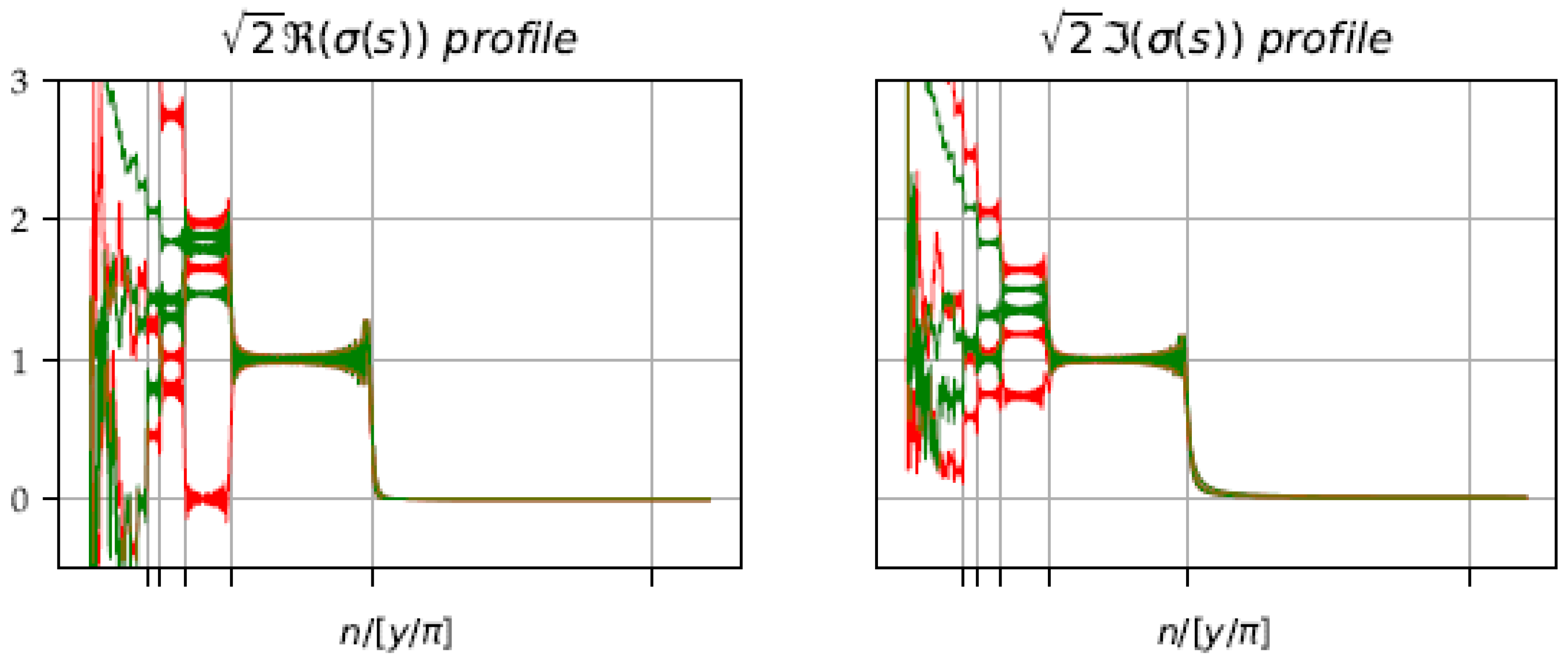
The purpose of the primitive observation is to optimize the visualization of surfaces and curves. We define a transformation on the graphs, in order to standardize the entities, to tame the general appearance and to calibrate the local behaviors. Thus, we convert the graph of the ζ function via anamorphosis, by a homothety of ${\left[y/2\pi \right]}^{\left(s-1\right)/2}$ and that of sums ${\sigma }_n$, is converted into a common profile after $n_{¼}=[y/4\pi ]$, via a translation and homothety ($-\zeta \left(s\right);{\left[y/2\pi \right]}^{x-½})$.

3.1.1. The Surfaces $C\left(x,y\right) \mathrm{and} S\left(x,y\right)$: Parallel Folds in $y$, the Functional Correspondence in $x$

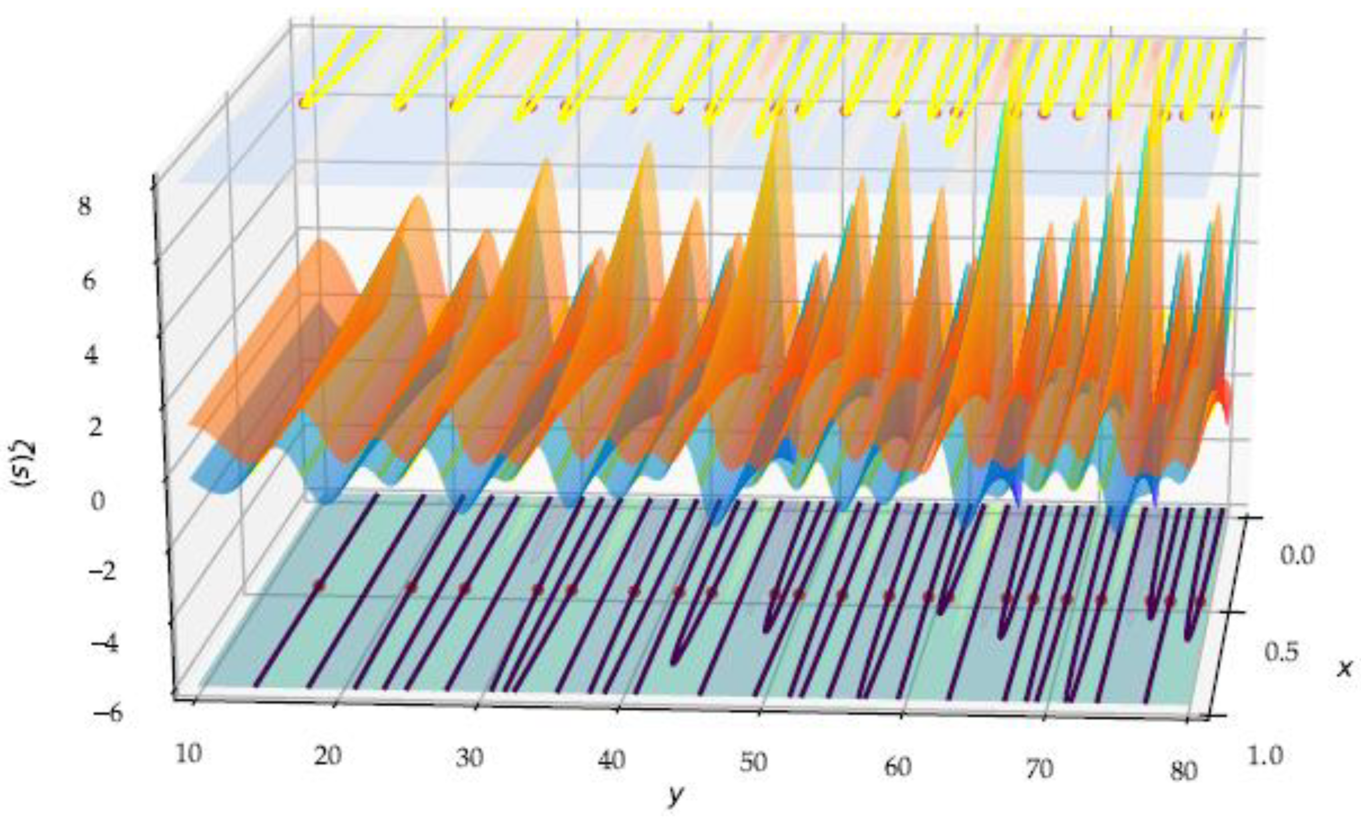
The $\zeta$ function derives from ‘nice underlying functions’. Figure 1 shows both functions $C\left(x,y\right) \mathrm{and} S\left(x,y\right)$ which have a similar morphology of irregularly corrugated fabric. Functions are smooth, in folds parallel to $y$, more and more tight from left to right as $y$ increases, and progressively weak from back to front ($x \mathrm{from} 0 \mathrm{to} 1$). The 0-level curves of each of the surfaces $C \mathrm{and} S$ are often located, in the valleys of the cosine, halfway up the undulations of the sine, where the function presents neither singularity nor any exceptional geometrical property (Figure 2).

The RH is not due to mathematical singularities. It is not to be explored in the peaks of the folds, but in the intrinsic properties of the functions themselves, namely the sum of concrete functions (logarithm, trigonometric, power) which are involved in the calculation. We will therefore abandon the analysis of the surface neighborhood and focus on the intrinsic analysis of each point $\left(x,y\right)$.

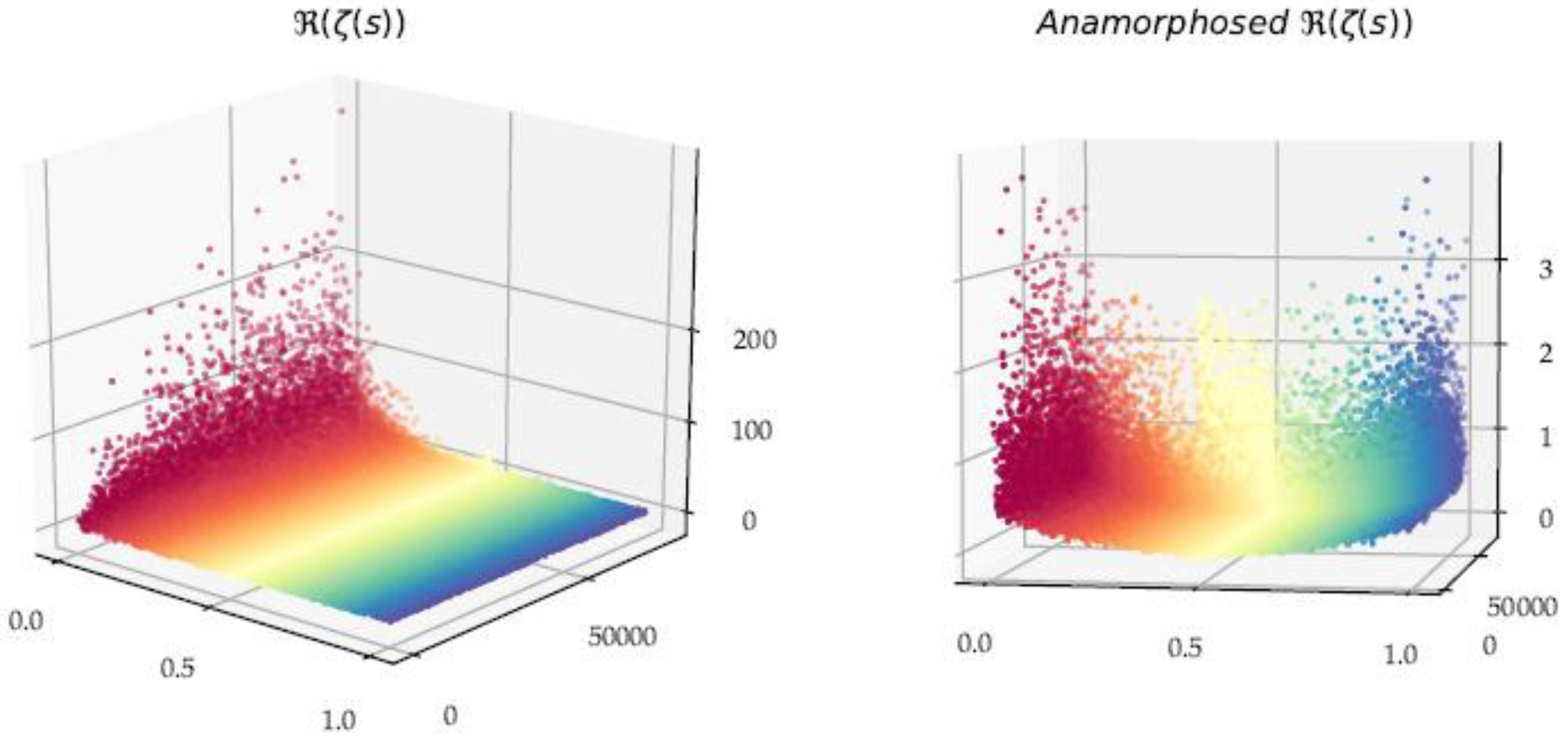
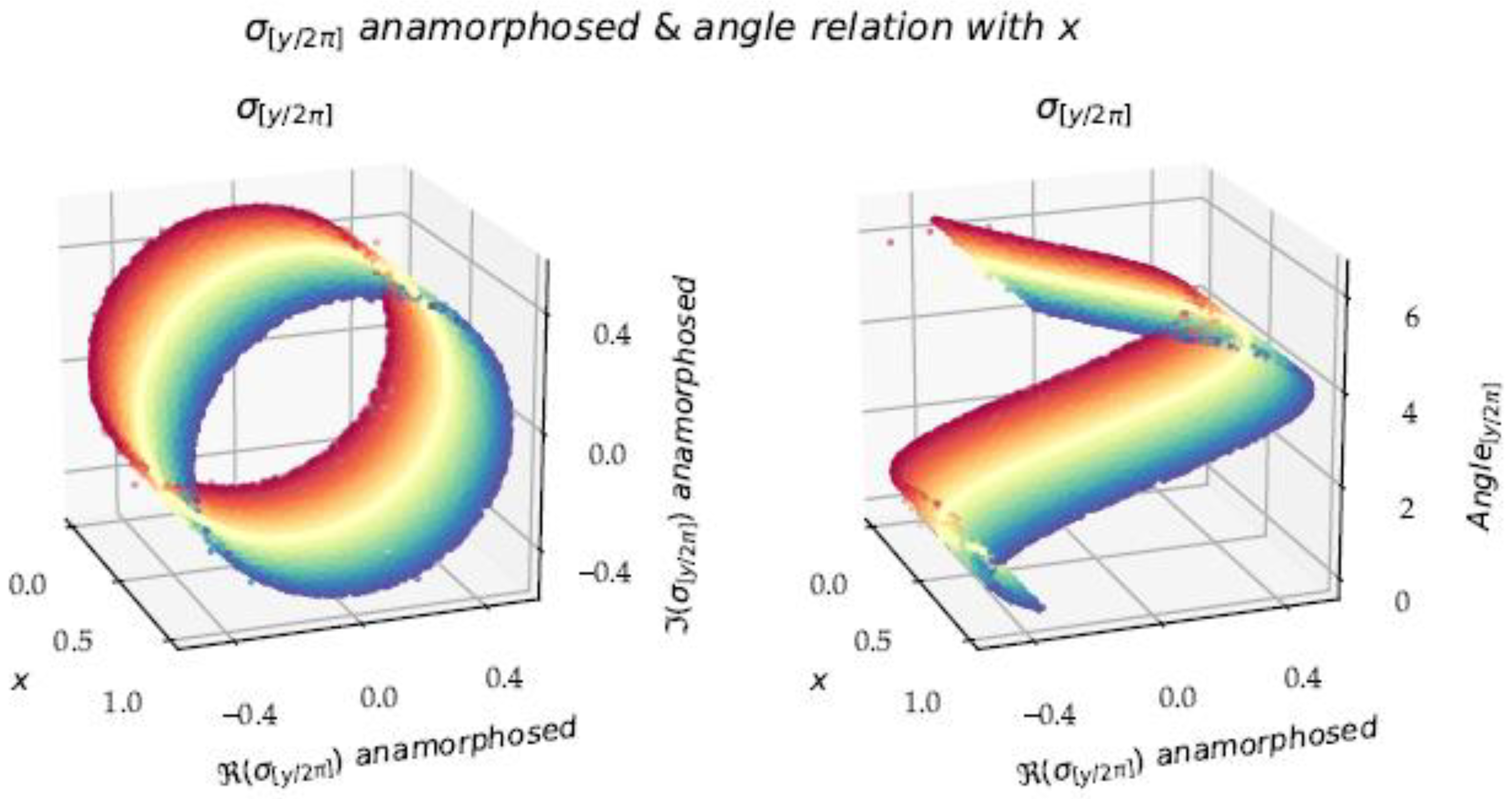
Figure 3 shows the anamorphosis of the $\zeta$ function to visualize the local behavior. The two different subsets $𝓩$ and $𝓦$ of the critical line $𝓛$ at $x=½$. are visible in light yellow color.

3.1.2. The Curves ${\sigma }_n\left(s\right)$: A Common Profile after Translation-Homothety

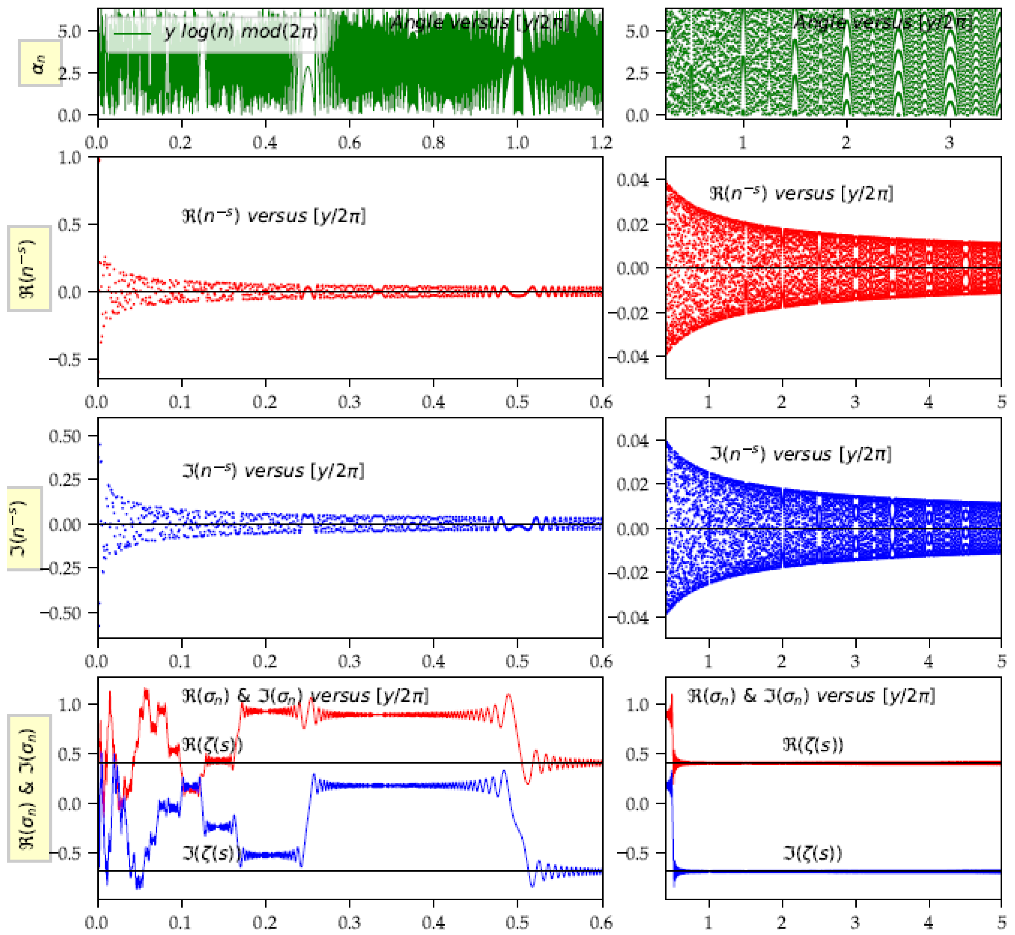
The term $z_n=n^{-s}=n^{-x}\left(cos\left\{\left[y log\left(n\right)\right]\mathrm{mod}\left(2\pi \right)\right\}-i sin\left\{\left[y log\left(n\right)\right]mod\left(2\pi \right)\right\}\right)$ is expressed in computation, as a function of the logarithm, of the cosine and sine, and of an angle measured with the $2\pi$ scale.

Figure 4 shows successively the curves, with abscissa $n/\left[u\right]$, where the importance of the angle ${\alpha }_n=ylog\left(n\right)modulo 2\pi$, appears on the terms $z_n$ and on the curves ${\sigma }_n\left(s\right)$. We also note the sequence, called harmonic, $𝓗:=\left\{[y/h\pi \left] {\displaystyle \cup } h[y/\pi \right]\right\}, h\in \mathbb{N},$ of aliasing indices, distinguishing the parity of $h$. When $h$ is even, the curve ${\sigma }_n$ has sharp fractures, due to cosine and sine aggregations of the same sign. The limit $\zeta \left(s\right)$ seems only to be built from the addition of these breaks, although it is difficult to identify them at the beginning of the n weak indices. When $h$ is odd, the sums of cosine and sine are of alternating signs, and the curve ${\sigma }_n$ reveals some constrictions in implosion.

Oscillations are observed (Figure 4), these being greater around the discontinuities $𝓗$ of the partial sums ${\sigma }_n\left(s\right)$; these oscillations are similar to the Gibbs (or Gibbs–Wilbraham) [25] phenomenon of the Fourier series of the square wave, or of series of eigenfunctions (occurring at simple discontinuities), or of approximations of functions with jump discontinuities. These oscillations occur whenever the function is discontinuous, and will be present whenever ${\sigma }_n$ meets a substantial jump. Here, they originate from the local influence of the sums of truncated trigonometric functions.

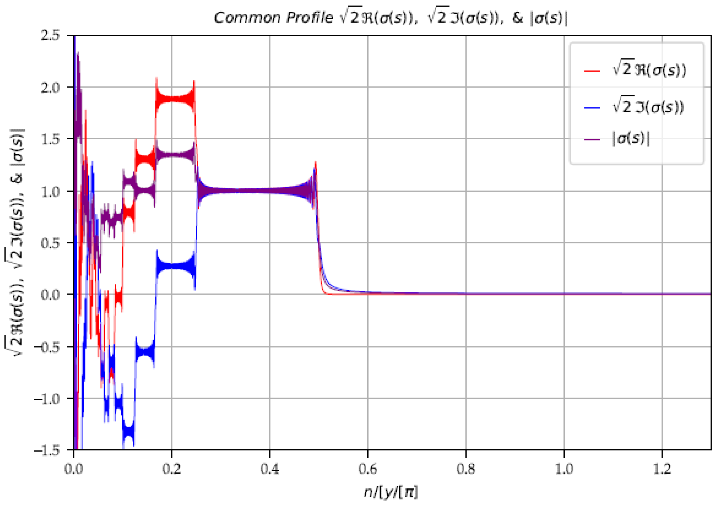
From all these observations, we are able to define a common profile (Figure 5), along the abscissa $n/\left[u\right]$, with an anamorphosis of the partial sums, defined by a translation-homothety.

For each of the profiles, one untangles the curves, after the index $n_{¼}$, by practicing successive rotations on ${\sigma }_n\left(s\right):$ $e^{i\left({\alpha }_n+\frac{y}{2n}\right)} \mathrm{if} n⩾n_{½ }\mathrm{and} e^{i\left({\alpha }_{½}+\pi \right)} \mathrm{otherwise}$. We thus make sure that $\Re \left({\sigma }_n\left(s\right)\right)$ is low after $n_{½}$ and we thus transpose the whole contribution of ${\sigma }_n\left(s\right)$ on $\Im \left({\sigma }_n\left(s\right)\right)$, which avoids working in ${ℝ}^2$. On Figure 6, we visualize $\sqrt{2}{\sigma }_n\left(s\right)$ to display the common profile for different $s$.

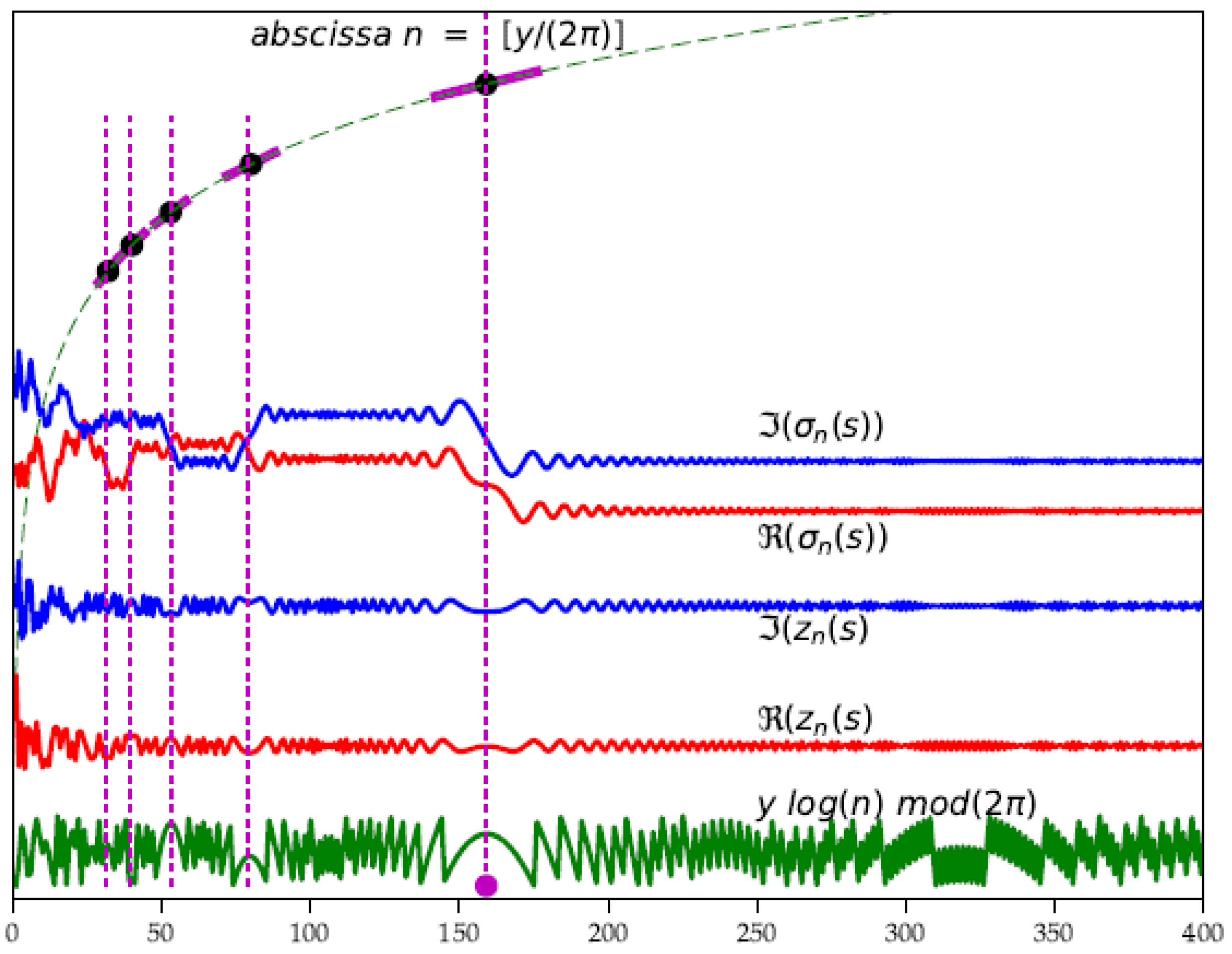
3.1.3. The Curves ${\sigma }_n\left(s\right)$ in Polar Coordinates: Helix Aliasing with the Change of Direction

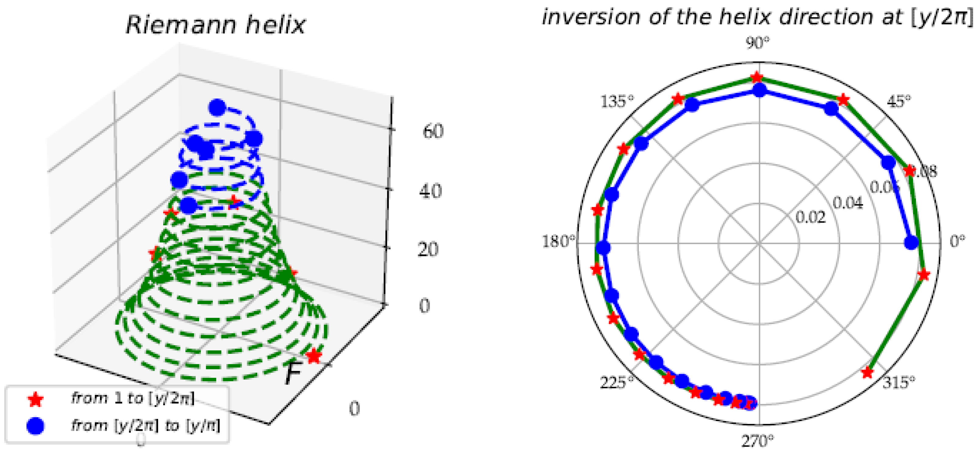
An unusual phenomenon occurs by the $2\pi$ modularity of the logarithmic function. When the derivative $y/n$ of the function $y log\left(n\right)$ is equal to 1, (and its harmonics equal to $1/h$) the cosines and sines are distributed before and after on the trigonometric circle, but the angle ${\alpha }_n$ reaches a maximum angle and the sequence of angles reverses and retraces its steps. This phenomenon of inversion of the direction on the trigonometric circle, in fact generates the limit values of the $\zeta$ function (Figure 7). This inversion appears on the sampled set, but not on the continuous helix.

3.2. Anatomy of the Components: Angle α and the Fresnel Cliffs and the Clothoids

3.2.1. The Terms $z_n$: Inevitable Memory of the Logarithm and the Angle $\alpha$

We summarize the key effect of the logarithm on Figure 8, where the $𝓗$ harmonic sequence emerges in all the different curves.

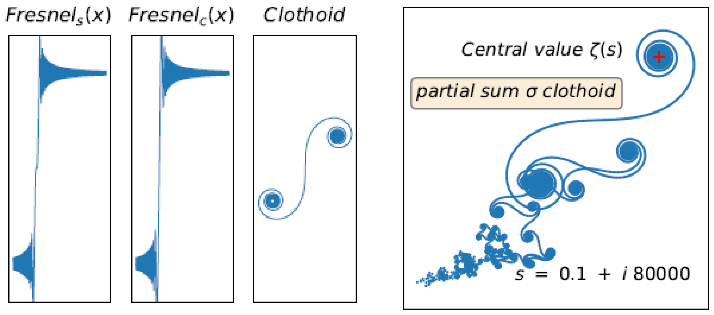
3.2.2. Fresnel’s Patterns ${{\displaystyle \sum }}_{k=-p}^p{e}^{i(a+b{k}^2)}$ and the Sums ${\sigma }_n$ in the Shape of 2D Clothoids

The morphology of the partial sums ${\sigma }_n$ is explained by Taylor’s formula

$$\begin{gathered} y log\left(\left[y/h\pi \right]+p\right)=y log\left(\left[y/h\pi \right]\left(1+p/\left[y/h\pi \right]\right)\right)\simeq y log\left(\left[y/h\pi \right]\right)+ph\pi -p^2{\left(h\pi \right)}^2/\left(2y\right)+\dots , p\in \mathbb{Z} \\ ylog\left(\left[y/h\pi \right]+p\right)={\alpha }_{n_{1/h}}+\epsilon \pi -p^2{\left(h\pi \right)}^2/\left(2y\right)mod 2\pi , p\in \mathbb{Z}, \epsilon =0 \mathrm{if} \mathrm{ph} \mathrm{is} \mathrm{even}, \mathrm{otherwise} \epsilon =1. \\ cos\left(ylog \left(\left[y/h\pi \right]+p\right))=\epsilon cos({\alpha }_{n_{1/h}}+\beta p^2\right), \epsilon =1 \mathrm{if} \mathrm{ph} \mathrm{est} \mathrm{even}, \mathrm{otherwise} \mathrm{alternatively} \epsilon =\pm 1. \end{gathered}$$

The point $n=\left[y/\left(2\pi \right)\right]$ thus makes it possible to define ‘even harmonics’: $n_h=\left[y/\left(2h\pi \right)\right]$ for the $\zeta$ function (For the $\eta$ function, they are odd: $n_h=\left[y/\left(\left(2h+1\right)\pi \right)\right])$. Around these points, the finite sums generate clothoids. These clothoids are caused by the regular and ‘clumsy’ sampling of the sequence of integers $u_n=n,n\in \mathbb{N}$ compared to the sequence $v_n=log\left(n\right)$, a hiatus which produces an aliasing by a stroboscopic effect of the usual trigonometric functions, sine and cosine. It appears as ‘Fresnel cliffs’, named this way by analogy to the eponymous integrals (Figure 9).

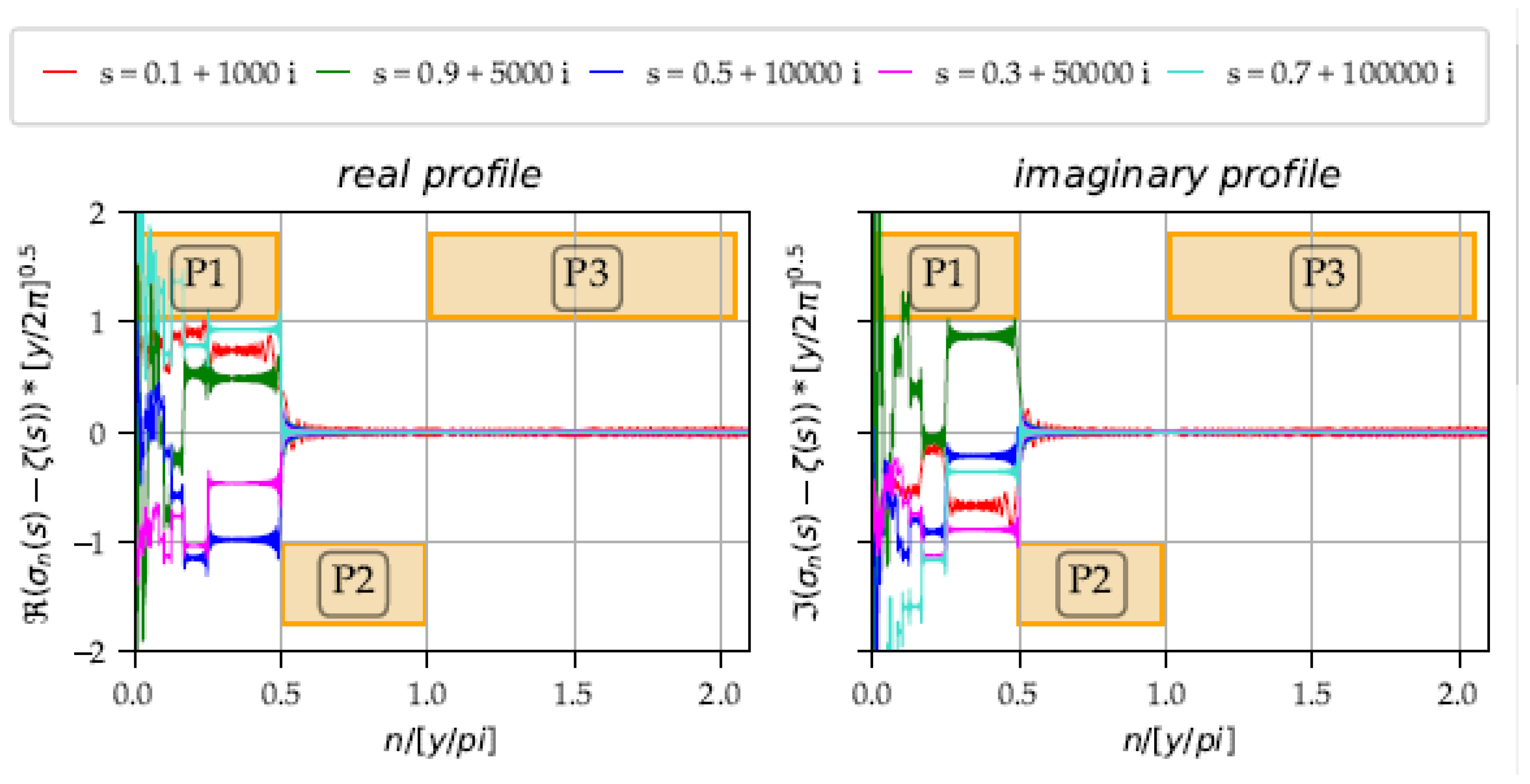
3.3. Morphology of the Partial Sums of the Series Split in 3 Phases in the Critical Strip

Discovery and development of formulae required a lot of interactive research effort, including higher order developments. In formulae, $[y/(2\pi )]$ and $t=y/\left(2\pi \right)$ must be distinguished, as the results become different. The estimator depending on the index $n_1$ gives the best accuracy. The errors made on the estimates are fairly small. This makes it possible to quickly visualize curves and surfaces with these estimators when exactness is not required, since the calculation of ${\zeta }^{\ast }$ is essentially condensed to a sum of $[y/\pi ]$ terms. Formulae, according to other indices, have been developed: $e.g. \forall s\in 𝓢: {\sigma }_{n_3}-\zeta \left(s\right)\simeq z_{n_3-1}$.

In the critical strip, all the partial sums have, whatever $x \mathrm{and} y$, an analogous behavior that we analyze in order to derive properties whose origin is in the anatomy of the elementary functions that compose their terms, namely the modulo $2\pi$ logarithm function, the two trigonometric cosine and sine functions and the power function. We thus highlight two particular indices that are of decisive importance. They split all the indices of the natural numbers into three dissimilar regions due to the effect of the regular sampling (and consequently inadequate for a good representation) of the continuous function by the natural numbers. This constant-interval sampling then causes staggering on the modulo $2\pi$ logarithm function. This aliasing effect has structuring consequences on the partial sums and on the morphogenesis of the Riemann function. The three phases of evolution are as follows.

3.3.1. Phase $P_1$: Gestation of the Limit $\zeta \left(s\right)$

The first phase $P_1$, erratic, itself is divided into two cycles, a jerky, spasmodic cycle, and a harmonic cycle of longer and longer plateaus, separated by ruptures, like cliffs, in the form of Fresnel functions. In phase $P_1$, the partial sums ${\sigma }_n$, influenced by the first values $z_k$, already register and memorize the final limit. The limit $\zeta \left(s\right)$ is an endogenous character of this phase $P_1$. More precisely, the gestation of the limit ends at point $n_{½}=\left[y/2\pi \right]$. It is at this point that the conjecture may be proved. In the critical strip, behaviors are similar to a homothetic factor beyond $n_{½}=\left[y/2\pi \right]$.

Figure 10 shows the relationship between $\left({\sigma }_{n_{½}}\left(s\right)-\zeta \left(s\right)\right) {n_{½}}^{x-½}$, the angle ${\alpha }_{n_{½}}$ and $x$ at the first order. Figure 11 (left panel) shows the discrepancy vis-à-vis the theoretical model, at the first order. It is necessary to go further and to improve the approximation formula with the residual $\{y/2\pi \}$. Laborious interactive work gives the final formula, with higher order corrections. From the 3D plots, at $n_{½}=\left[y/2\pi \right]$, we can finally establish the first order (6) and the final (7) approximation formulae for the phase $P_1$: $\forall s=x+iy\in 𝓢$

$$2\left(\zeta \left(s\right)- {{\displaystyle \sum }}_{n=1}^{n_{½}}{n}^{-s}\right)\simeq z_{n_{½}}{e}^{i\pi ¼}\sqrt{n_{½}}={n_{½}}^{-s+½}{e}^{i\pi ¼}={n_{½}}^{-x+½}{e}^{-i\left({\alpha }_{n_{½}}-\pi ¼\right)}$$

(6)

$$\zeta \left(s\right)={{\displaystyle \sum }}_{n=1}^{n_{½}}{n}^{-s}+{n_{½}}^{-s}\left(½e^{i\pi ¼}\sqrt{n_{½}}+\left\{t\right\}-½-i\left(x-½\right)/2\pi -p {n_{½}}^{-½}+𝓞\left({n_{½}}^{-1}\right)\right)$$

(7)

3.3.2. Phase $P_2$: Emergence of the Functional Equation ξ

The middle phase $P_2$ is a transition and decompensation phase. The sampling is more precise, the angle $\alpha$ in polar coordinates becomes less irregular and organizes a morphology of damping, of smothering, and a beginning of convergence. In the $P_2$ phase, on the other hand, the intermediate sum will not intrinsically memorize the final limit, which has been erased from the calculations, since the $P_2$ phase has lost the knowledge of the terminal target. On the other hand, the Dirichlet sum begins its convergence from this phase $P_2$.

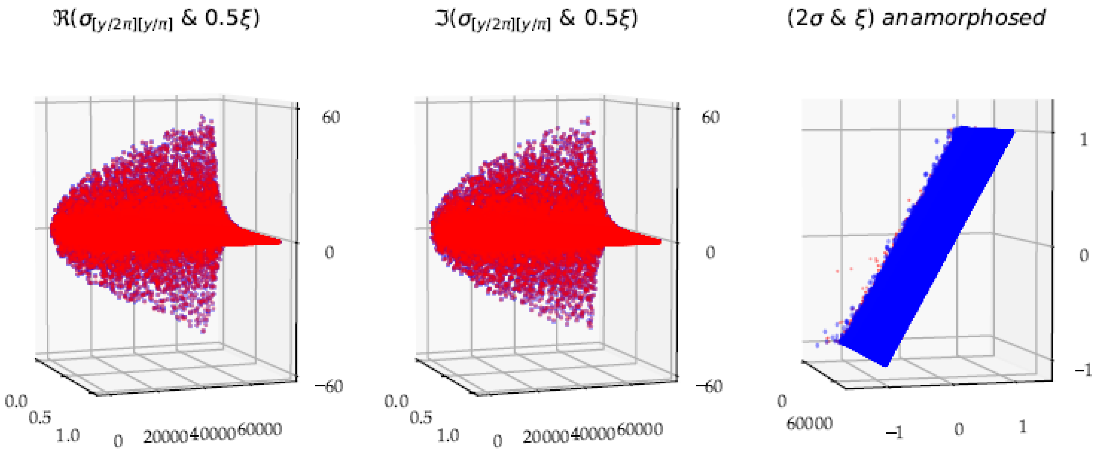
Figure 12 shows the relationship between ${{\displaystyle \sum }}_{1+n_{½}}^{n_1}{n}^{-s} \mathrm{and} ½\xi \left(s\right)$. The final formula with higher order corrections further improves the approximation. Therefore, we establish the first order (8) and the final (9) approximation formulae for the phase $P_2$, $\forall s=x+iy\in 𝓢$

$$2{{\displaystyle \sum }}_{n=1+n_{½}}^{n_1}{n}^{-s}-\xi \left(s\right)\simeq {n_1}^{-s}=z_{n_1}$$

(8)

$${n_{½}}^s{{\displaystyle \sum }}_{n=1+n_{½}}^{n_1}{n}^{-s}=½ {n_{½}}^s\left(\xi \left(s\right)+{n_1}^{-s}\right)+\left\{t\right\}-½-i\left(x-⅔\right)/2\pi +𝓞\left({n_{½}}^{-1-s}\right)$$

(9)

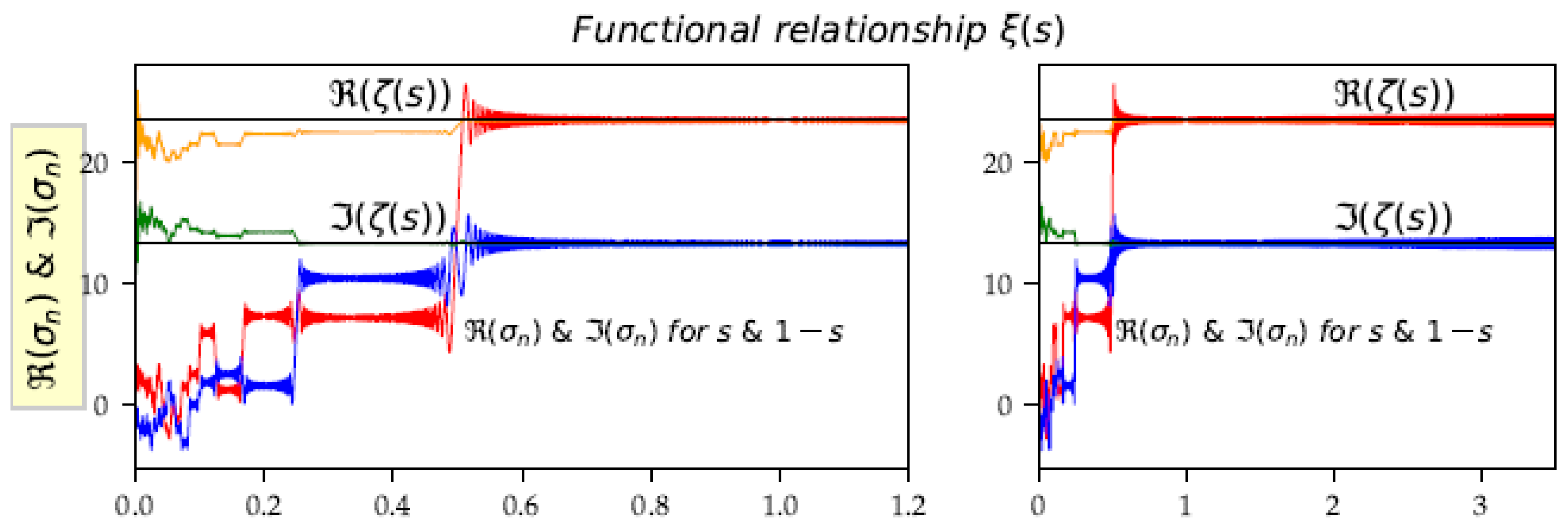
Figure 13 shows the effects of the functional equation on the partial sums along $n/\left[u\right]$. Keeping in mind the metaphor of the curtain, the $\xi$ function is an anamorphosis which makes it possible to connect the folds from above and below the curtain. In the symmetry middle $x=½$, this prism is neutral. The $\xi$ function serves to maintain this direct relationship between the great and small gathers of Riemann’s curtain.

It is thus important to detect this functional equation within the partial sums. This equation emphasizes the link between the values $\zeta \left(s\right) \mathrm{and} \zeta \left(1-s\right)$, but the partial sums of the functions $\zeta \left(s\right) \mathrm{and} \zeta \left(1-s\right)$ behave differently, at the level of the angles, of the plateau values, and oscillation amplitudes. Nevertheless, the central values of oscillations starting from $[y/2\pi ]$ are identical to ensure the equality of the limits.

3.3.3. Phase $P_3$: Divergence of $\zeta$ Riemann and the Convergence of $\eta$ Dirichlet

Figure 14 shows the relationship between $\left({\sigma }_{n_1}\left(s\right)-\zeta \left(s\right)\right) {n_1}^x$, the angle ${\alpha }_{n_1}$ and $x$ at the first order. There are some discrepancies (Figure 11, right panel). The final formula with higher order corrections further improves this approximation. At $n_1=\left[y/\pi \right]$, we finally establish the first order (10) and final (11) approximation formulae for the phase $P_3$, $\forall s=x+iy\in 𝓢$

$$\forall s=x+iy\in 𝓢: 2\left(\zeta \left(s\right)-{{\displaystyle \sum }}_{n=1}^{n_1}{n}^{-s}\right)\simeq -{n_1}^{-s}=-z_{n_1}$$

(10)

$$\forall s=x+iy\in 𝓢: \zeta \left(s\right)={{\displaystyle \sum }}_{n=1}^{n_1}{n}^{-s}+{n_1}^{-s}\left(-½+\left(x+i\pi \left\{u\right\}\right)/4n_1+𝓞\left({n_1}^{-1}\right)\right)$$

(11)

The terminal phase $P_3$ generates divergence. These are ripples becoming larger and larger, and wider and wider. Soon the functions are sweeping intervals that will reach higher and higher values in the positive and negative directions. In fact, the logarithmic function greatly lengthens the $2\pi$ increment intervals, which generates a roller coaster by an accumulation of more and more numerous terms of very similar trigonometric values, the power function playing only a second homothetic role. Phase $P_3$ is a phase of divergence, of oscillations around a central value, which is in fact the limit of the meromorphic function. It is the value most often traversed by scans of sigma functions. The infinite sum of Dirichlet of this phase $P_3$ makes it possible to calculate this central value. $P_3$ determines the exact values of $y_{izero}$ on the critical line.

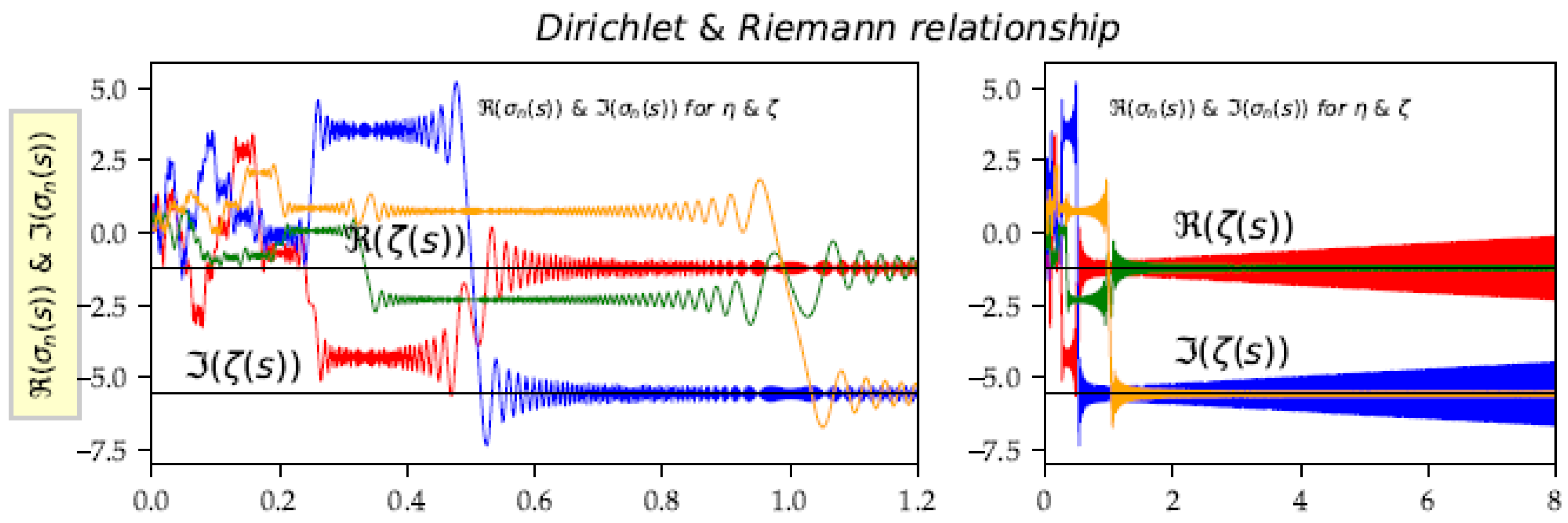
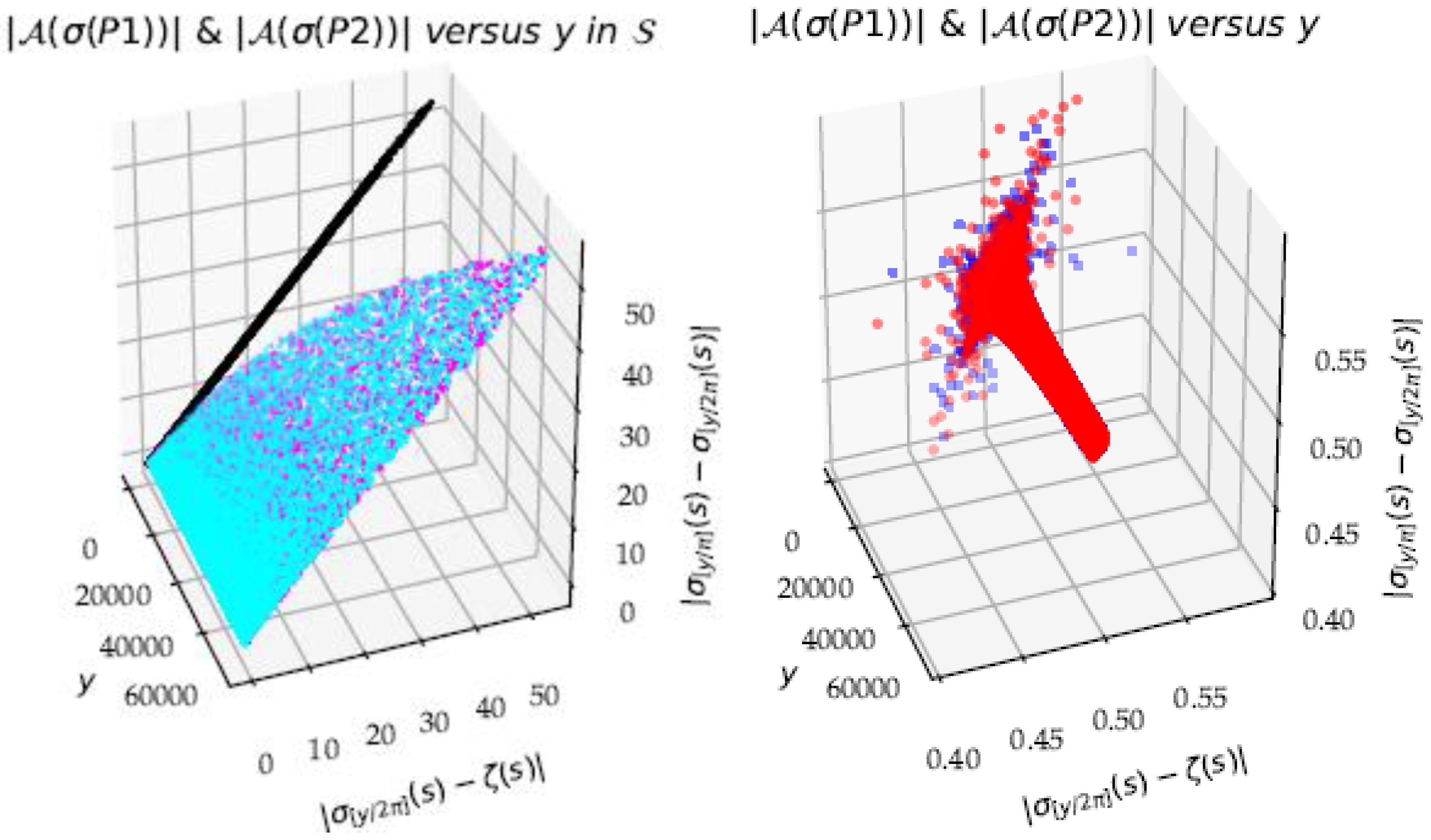
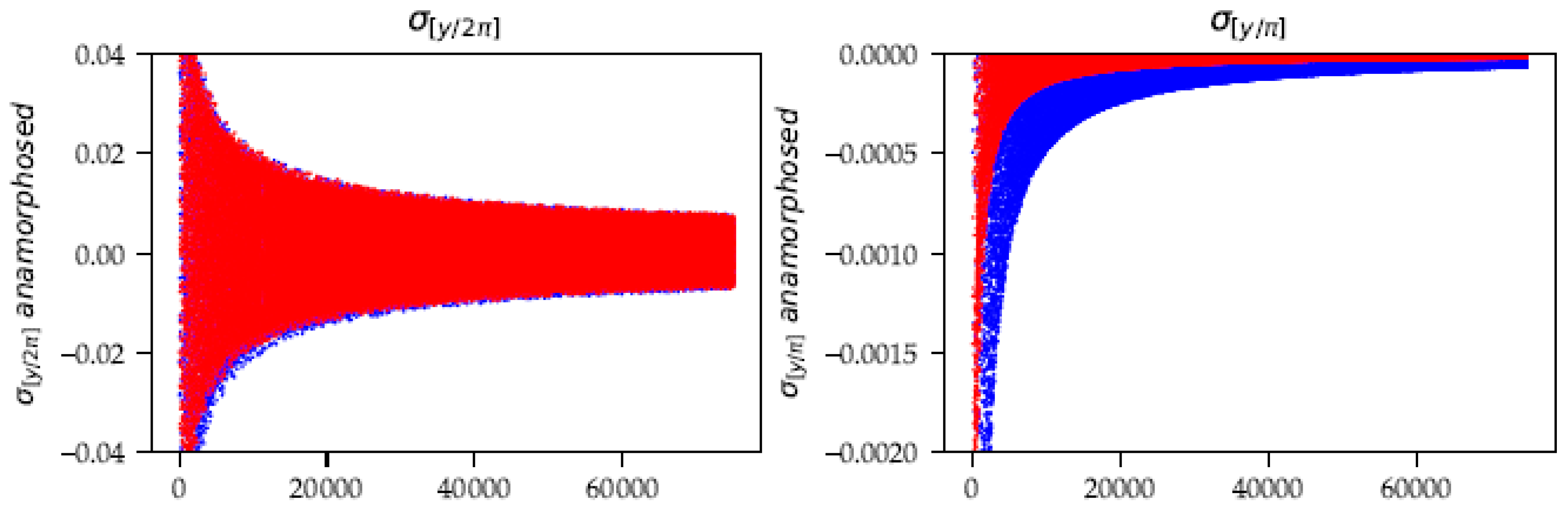
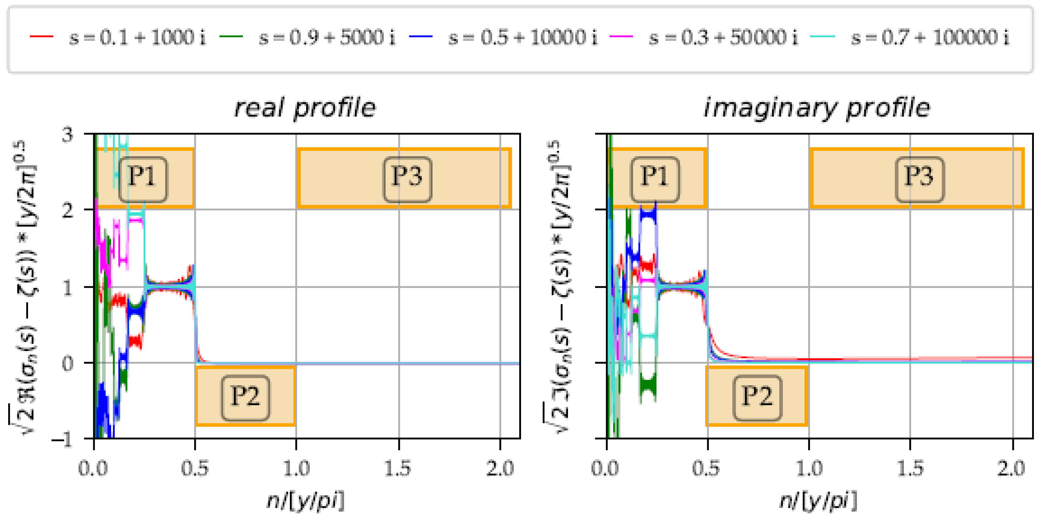
It is important to understand the interrelation between $\zeta \left(s\right)$ and $\eta \left(s\right)$ in the critical strip, by analyzing the partial sums of both functions (Figure 15). Their behavior is similar in phases $P_1$ and $P_2$, except that the phases correspond to double indices for $\eta$ with respect to $\zeta$. On the other hand, in the $P_3$ phase, the $\zeta$ function diverges irreparably, while oscillating around a ‘central value’, which is a median value of oscillation, whereas the $\eta$ function converges uniformly towards a true limit $\eta \left(s\right)=\zeta \left(s\right)\left(1-2^{-s+1}\right)$. The $\zeta$ function is a sum that can be estimated by an integral when the functions $sin\left(ylog\left(n\right)\right) \mathrm{and} cos\left(ylog\left(n\right)\right)$ are ‘well discretized’ from $n>N\left[y/\pi \right]; N \mathrm{large}$. The sum ${\sigma }_n\left(s\right)$ then reacts as an integral of a continuous function $Z\left(s\right)={{\displaystyle \int }}_1^{\infty }1/z^{s}dz$. After the value $[y/\pi ]$, a phenomenon takes place, more violent than the Cesàro’s arithmetic mean situation. The positive and negative sub-sums win out one after the other and we witness a more and more pronounced rollercoaster phenomenon. It would be advisable to define a ‘convergence’ for this divergent sum, via the central value. Although the Cesàro subsequences diverge, we can statistically define the central value of the undulations or consider the involute center of the 2D spiral generated by the real and imaginary parts of $\zeta$, ($\zeta \left(s\right): \mathrm{clothoid} \mathrm{center})$. (See Figure 9, right panel).

3.4. The Three Nested Domains: Presence of ½ in the Exponents of Homotheties

We have established valid relations in the critical strip, $\forall s\in 𝓢$, with an estimation of the errors which are of the order of $y^{-\left(s+1\right)}$, which reinforces us towards a general result for the values of $s$ with a higher $y$. At the first order of magnitude, we have the three formulae for the three phases

$$\forall s=x+iy\in 𝓢:({\sigma }_{n_{½}}\left(s\right)-\zeta \left(s\right)){n_{½}}^{x-½}\simeq -½ e^{-i\left({\alpha }_{n_{½}}-\pi /4\right)}$$

(12)

$$\forall s=x+iy\in 𝓢:\left({{\displaystyle \sum }}_{n=1+n_{½}}^{n_1}{n}^{-s}-½\xi \left(s\right)\right){n_1}^x\simeq ½ e^{-i{\alpha }_{n_1}}$$

(13)

$$\forall s=x+iy\in 𝓢:\left({\sigma }_{n_1}\left(s\right)-\zeta \left(s\right)\right){n_1}^x\simeq ½ e^{-i{\alpha }_{n_1}}$$

(14)

On the critical line $𝓛$, the formulae (12) and (14) are simplified, thanks to the element $½$.

$$\forall s=½+iy\in 𝓛:{\sigma }_{n_{½}}\left(s\right)-\zeta \left(s\right)\simeq -½ e^{-i\left({\alpha }_{n_{½}}-\pi /4\right)}$$

(15)

$$\forall s=½+iy\in 𝓛:\left({\sigma }_{n_1}-\zeta \left(s\right)\right)\sqrt{n_1}\simeq ½ e^{-i{\alpha }_{n_1}}$$

(16)

The relationship (13) between the partial sums and the associated function is also simplified. Keeping in mind that $\xi \left(½+iy\right)\simeq e^{-i\left(y log\left(y/2\pi e\right)-\pi /4+⅜/y\right)}$ belongs to the unit circle, it becomes

$$\forall s=½+iy\in 𝓛: {{\displaystyle \sum }}_{n=1+n_{½}}^{n_1}{n}^{-s}=½ \left(\xi \left(s\right)+z_{n_1}\right)+(\left\{t\right\}-½+i/12\pi ){n_{½}}^{-s}+𝓞\left({n_{½}}^{-1½}\right)$$

(17)

The presence of the term $½$ in the exponent of the homotheties discriminates the nested domains $𝓢,𝓛,𝓩$. Its cancellation repairs the hiatus of the homothety ratios and the translation $-\zeta \left(s\right)$ balances the two phases $P_1 \mathrm{and} P_2$ for the set $𝓩$.

3.5. $𝓩$ Distribution of Non-Trivial Zeros on the Critical Line $𝓛$

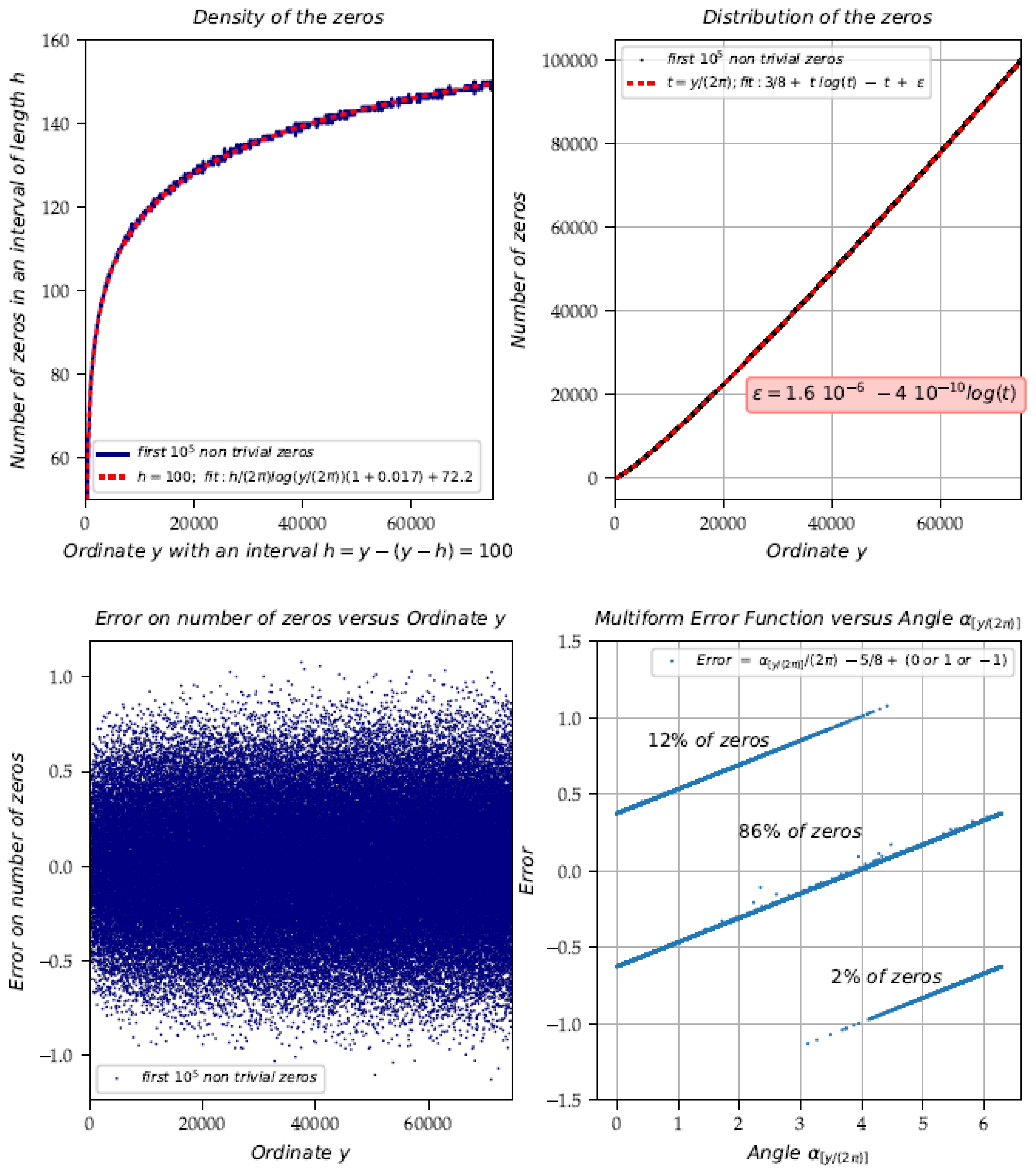
We specify the formulae of the density of zeros (4) and the distribution of zeros (5) on the critical line from the set of selected points (Figure 16). The density of zeros, calculated over an interval $h$, is $d\left(y\right)=h/2\pi log\left(y/2\pi \right)+constant\left(h\right)$. The distribution of zeros, that is to say the number of zeros $<y$ is the integral of this density, that is to say $N\left(y_{izero}<y\right)=tlog\left(t\right)-t; t=y/2\pi$. However, this formula must be corrected which causes errors dependent on the ${\alpha }_{[y/2\pi ]}$, so the final Formula (5) is: $N\left(y_{izero}<y\right)=tlog\left(t\right)-t-\frac{{\alpha }_{[y/2\pi ]}}{2\pi }+1$. This formula allows, for a given $y$, to correctly estimate the number of zeros in the interval 86% of the time, with an overestimate +1 (i.e., the next $y_{izero}$ is ‘late’) 12% of the time, and with an underestimate −1 (i.e., the next $y_{izero}$ has already appeared) 2% of the time. The Formula (5) $N\left(y_{izero}<y\right)=tlog\left(t\right)-t-\frac{{\alpha }_{[y/2\pi ]}}{2\pi }+1$ is more accurate than the traditional formula $N\left(y_{izero}<y\right)=\frac{y}{2\pi }ln\left(\frac{y}{2\pi e}\right)+⅜$, thanks to the expression ${\alpha }_{[y/2\pi ]}=ylog\left[t\right] mod\left(2\pi \right)$ taking into account the angle $y log\left[\frac{y}{2\pi }\right]mod\left(2\pi \right)$. With this additional correction, a good estimation is obtained 86% of the time, on average.

4. Discussion

4.1. Approximation Formulae

In this paper, three approximation formulae are proposed: (1) and (3) for $\zeta \left(s\right)$, (2) for $\xi \left(s\right)$.

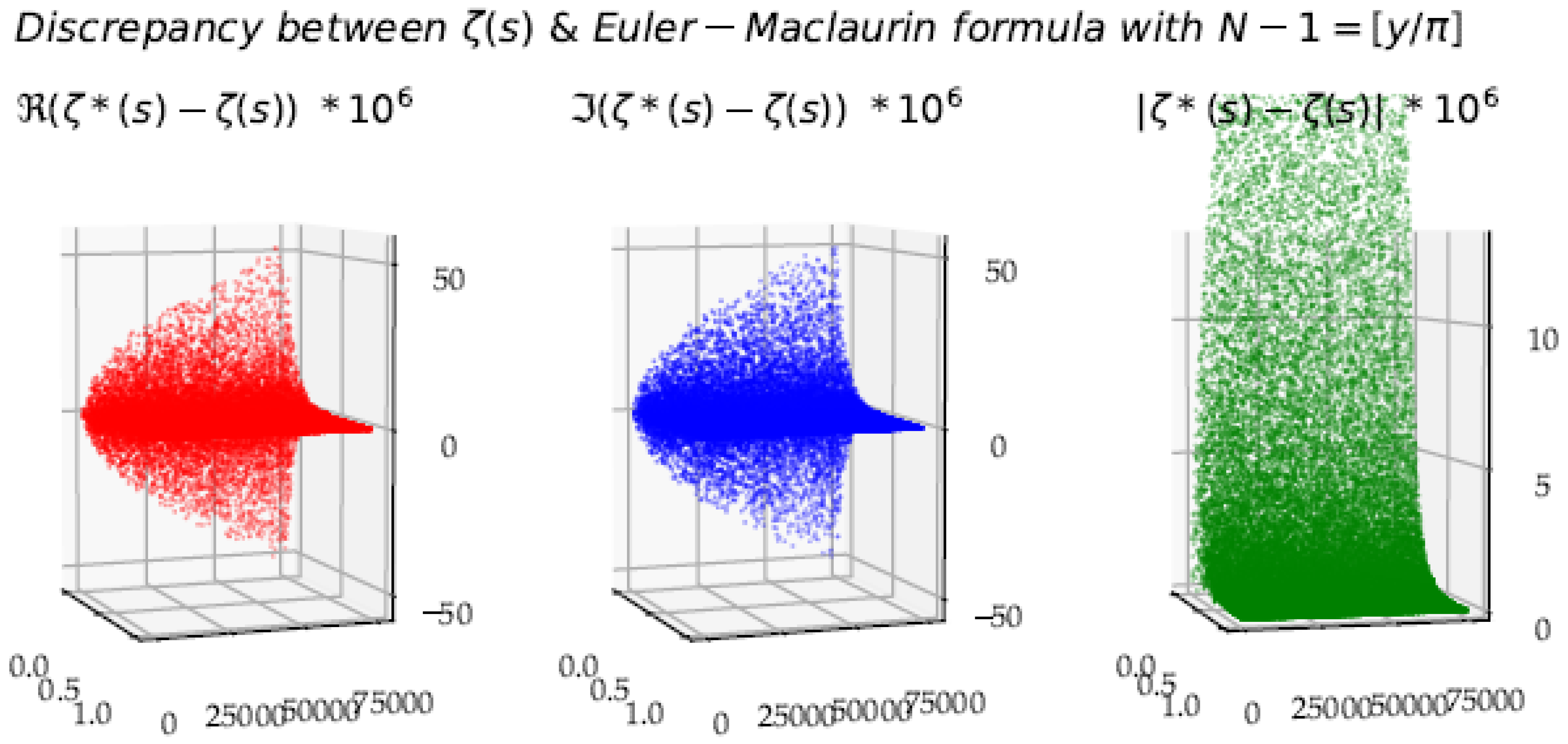
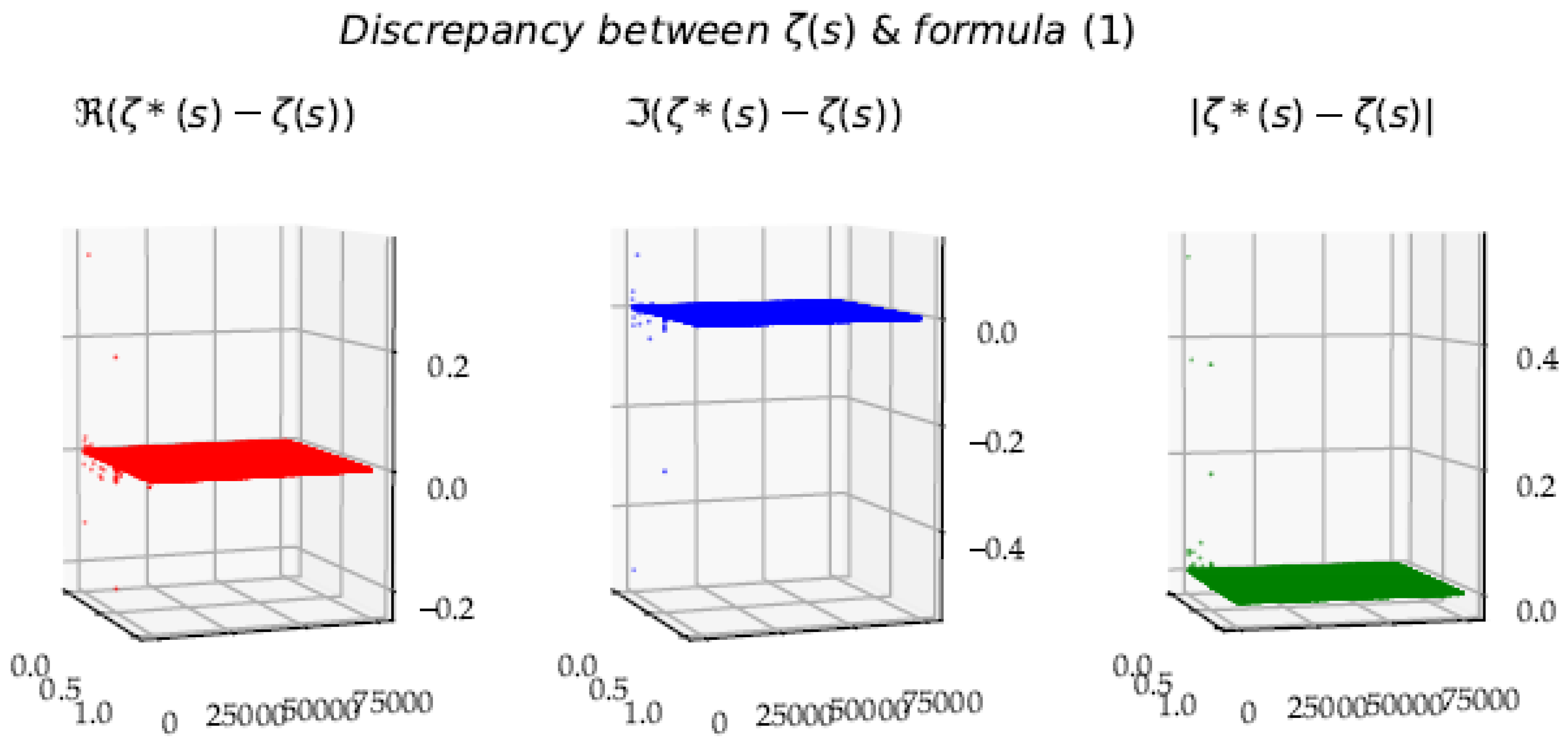
Figure 17 shows the discrepancy between the Formula (1) and $\zeta \left(s\right).$

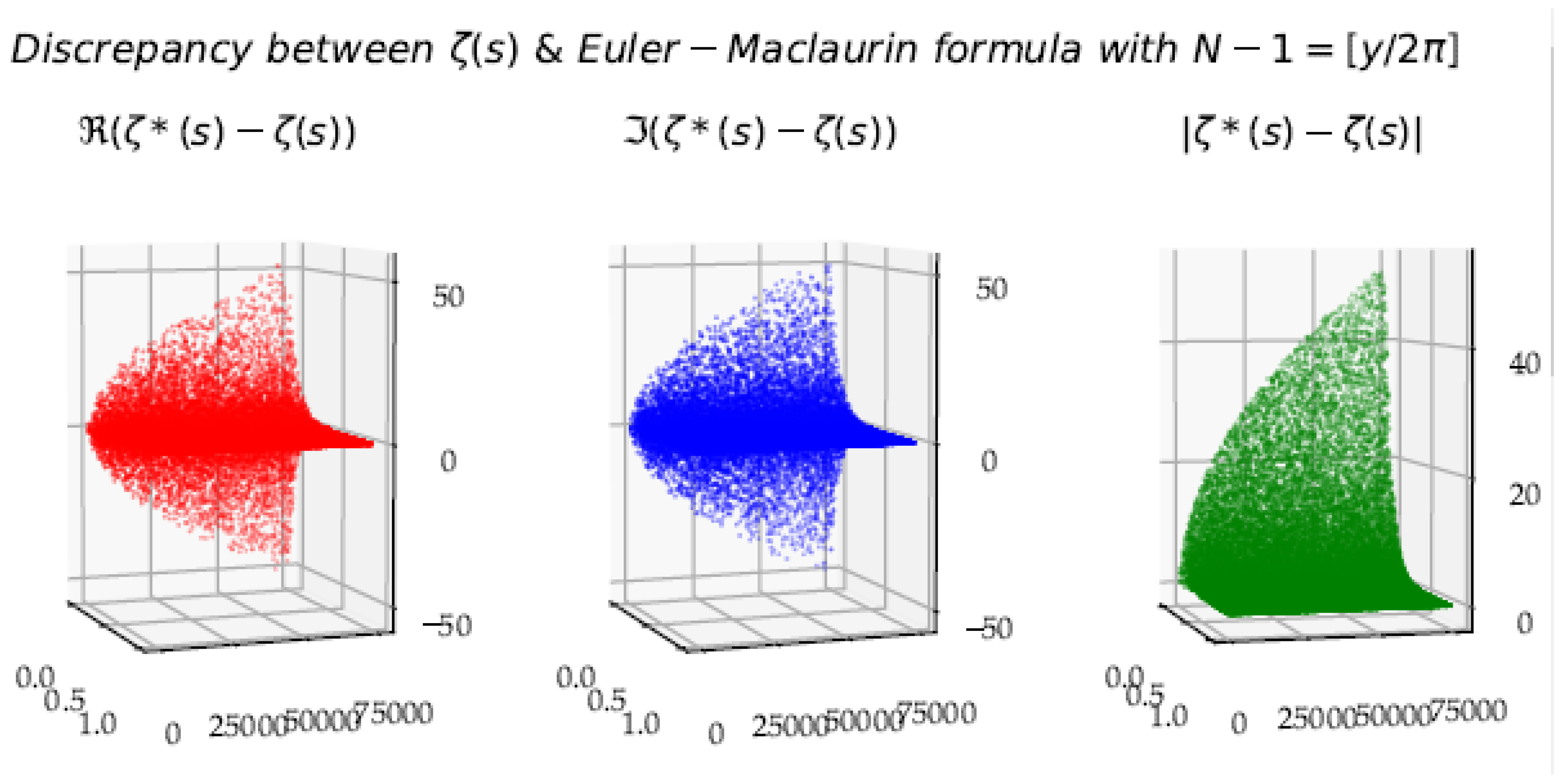
Figure 18 shows the discrepancy between the equivalent Euler–Maclaurin formula ($N-1=\left[y/2\pi \right]$) without the remainder and $\zeta \left(s\right)$.

Figure 17 shows that one can estimate $\zeta \left(s\right)$ with a reasonable approximation, using at least the first $n_{½}=\left[y/2\pi \right]$ terms.

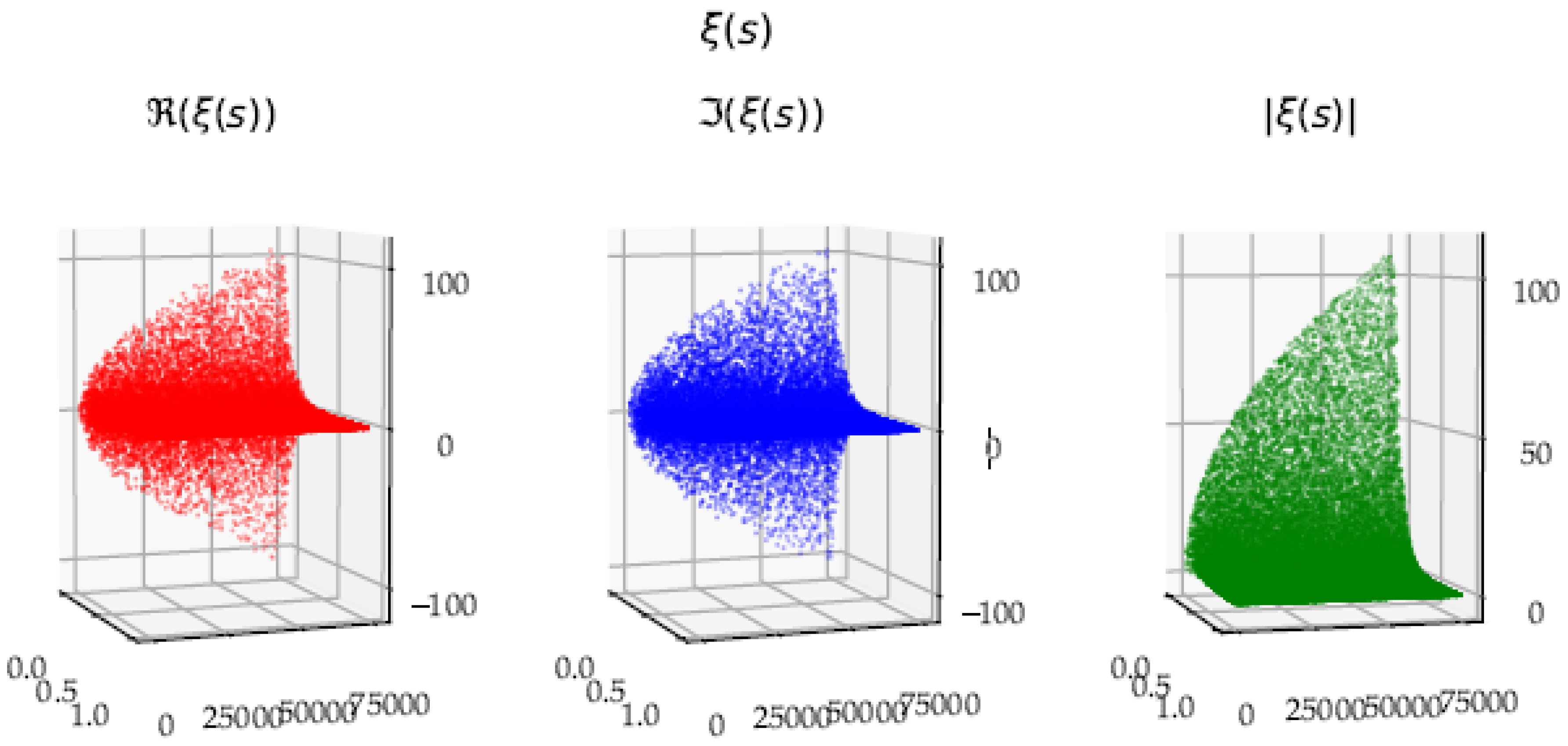
Figure 19 shows $\xi \left(s\right)$ for the $s$ values of the data points from $𝓕$, in the critical strip.

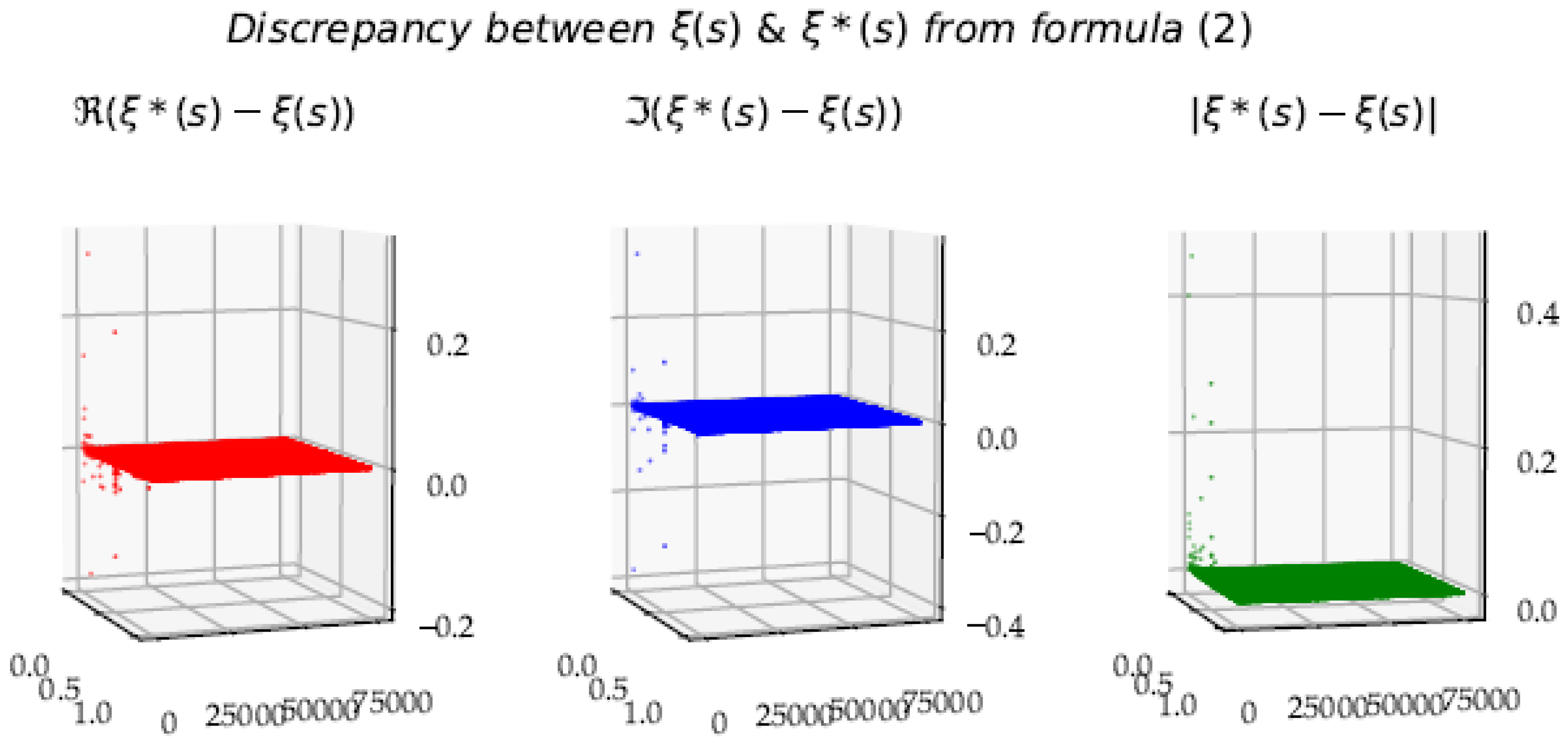
Figure 20 shows the discrepancy between $\xi \left(s\right)$ and the estimation ξ*(s) from Formula (2).

Figure 20 shows that it is possible to estimate $\xi \left(s\right)$ with a reasonable approximation, from the calculation of the partial sub-sum ${{\displaystyle \sum }}_{1+\left[y/2\pi \right]}^{\left[y/\pi \right]}{n}^{-s}$. Figure 20 emphasizes the intrinsic aspect of the $\xi$ function into the partial sub-sum of phase $P_2$.

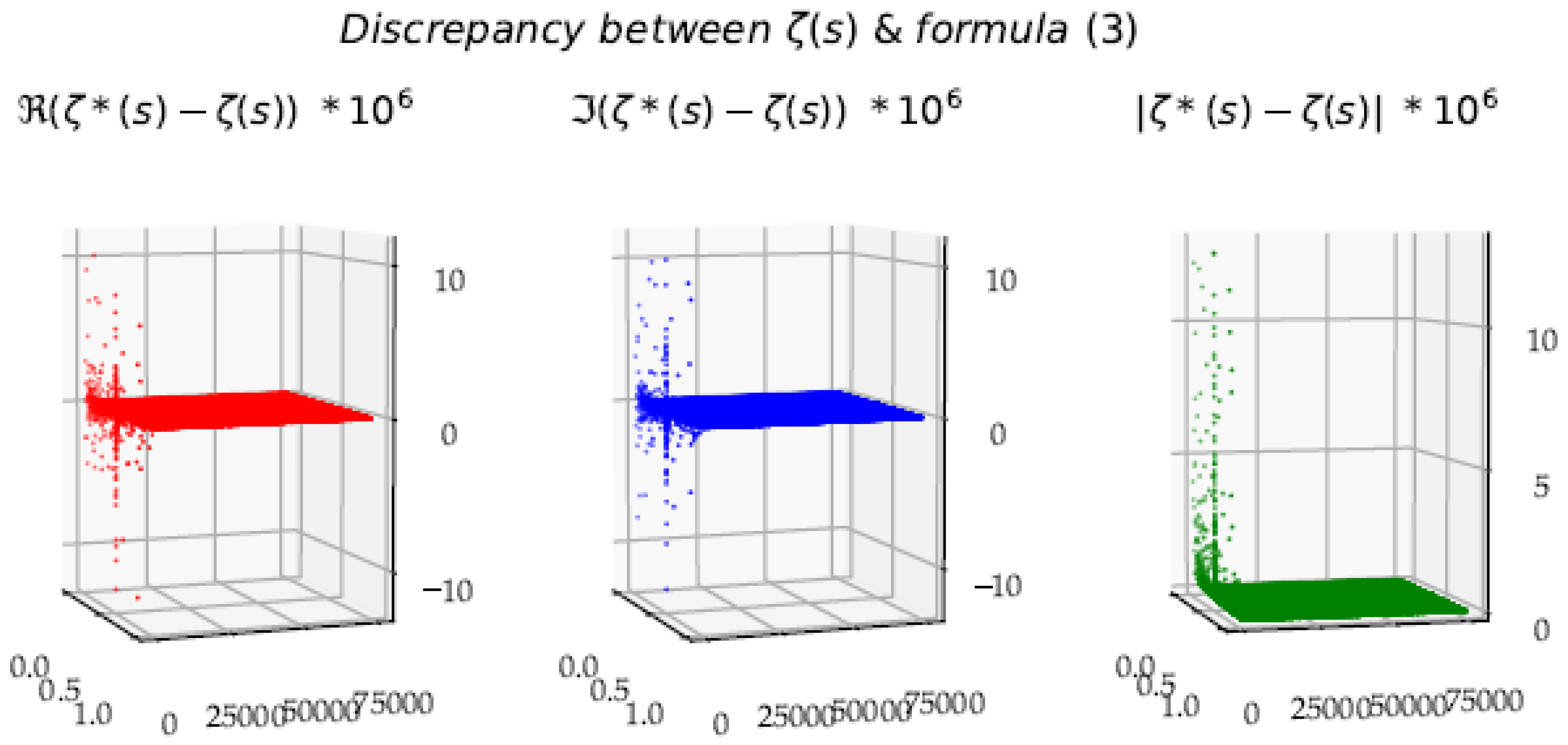
Figure 21 shows the discrepancy between Formula (3) and $\zeta \left(s\right)$.

Figure 22 shows the discrepancy between the equivalent Euler–Maclaurin formula ($N-1=\left[y/\pi \right]$) without the remainder and $\zeta \left(s\right)$.

Figure 21 shows that one can estimate $\zeta \left(s\right)$ with a quite good approximation, using the first $n_1=\left[y/\pi \right]$ terms. From the comparison between Figure 21 and Figure 22, we see the interest of working directly on the raw values of the partial sums, without involving an artificial entity (the integral ${\displaystyle \int }dt/t^s$) which obscures the understanding of the production of the $\zeta \left(s\right)$ limit. Additionally, using a non-natural entity distributes the gap between the raw function and this entity in a non-structuring way. The essential reason for the gap of the Euler–Maclaurin formula without the remainder, comes from the fact that the $\zeta \left(s\right)$ limit is precisely made in the Fresnel cliffs, where the nonconformity between, on the one hand, the discrete function of the series and on the other hand the continuous function, can be filled only by the Poisson’s remainder, in the form of an integral.

The results with the Riemann–Siegel formula will not be shown here because the gaps are even larger than those of the Euler–Maclaurin formula.

4.2. Morphogenesis of Riemann’s Function

Thanks to these estimates, we can understand the RH by its construction in the partial sums. Three phases are identified in the morphogenesis (Figure 23 and Figure 24).

In order to remove the obstacle, in the Riemann’s function, from the precise calculation of the expression ${{\displaystyle \sum }}_{k=a+1}^b{k}^{-s}$, one splits the sum into intervals where the $a$ and the $b$ are of the form $\left[y/h\pi \right] \mathrm{or} h\left[y/\pi \right], h\in \mathbb{N}$. Thus, the partial sums can be broken down into three distinct phases $P_1, P_2, P_3,$ separated by the two indices $n_{½}=\left[y/2\pi \right] \mathrm{and} n_1=\left[y/\pi \right]$. These three phases play different roles in the gestation of the limit $\zeta \left(s\right)$ and in the RH. The first phase $P_1$ endogenously builds the limit $\zeta \left(s\right)$; the second phase $P_2$ reveals the functional equation $\xi \left(s\right)$, i.e., the symmetry between $s \mathrm{and} 1-s$; the third phase $P_3$ reveals the divergence of the series ${{\displaystyle \sum }}_{n=1}^{\infty }{n}^{-s}$, whereas in this third phase, the associated Dirichlet function $\eta \left(s\right)$ expresses on the contrary its convergence, limit $\eta \left(s\right)$, constructed in the combined phases $P_1{\displaystyle \cup }{P}_2$.

1. In the phase $P_1$, the value $\zeta \left(s\right)$ is generated, with the largest terms of the infinite sum.

The limit $\zeta \left(s\right)$ is therefore endogenous from the initial values from $1 \mathrm{to} \left[y/2\pi \right]$ (in fact, the result is reached as early as $\left[y/3\pi \right]$). The element $e^{i\pi /4}$, true rotation of the axes, intervenes in the formulae up to the index $n_{½}$ to compensate for the difference due to the unbalanced term $z_1=1+0.i$ (the fixed-point F of the helix $𝒽(𝓽)$) and to restore the equilibrium between both $\left(\Re , \Im \right)$ axes.

2. Then, the phase $P_2$, independent of the limit $\zeta \left(s\right)$, exhibits the functional equation $\xi$, which was masked by the landscape dynamics in horizontal plateaus and steep cliffs.

Phase $P_2$, phase of exhaustion and decompression, reveals the deep nature of the $\zeta$ function. The reciprocity of the functional equation $\xi$, i.e., the duality along the x-axis, demonstrated by Riemann, thus appears in the foreground. At point $n_1$ the phase $P_2$ ‘converges’, or rather is concretized in $\zeta \left(s\right)$. Phase $P_2$ makes it possible to correctly estimate the limit $\zeta \left(s\right)$ because we have fertilized the limit in $P_1$ and extinguished the functional equation $\xi$ in $P_2$. At a $-\zeta \left(s\right)$ translation, if the two phases $P_1$ and $P_2$ are equal in modulus, the sum vanishes in $n_1$ (to within $½ z_{n_1}$).

3. Phase $P_3$ closes the calculations, but does not have a structuring role.

The divergence begins at point $\left[y/\pi \right]+1$, in a roller coaster, (in fact the divergence really starts around $2\left[y/\pi \right]$). The last phase manages the ε, to ‘converge’ to 0 (to within a meromorphy). The set $𝓩$, neutral element of the affine homothety $𝓗=\left\{-\zeta \left(s\right);\left(1/n_1, {n_{½}}^{\left(x-½\right)}\right)\right\}$, can only be included in the critical line $𝓛$, since $\left|\xi \left(s\right)\right|=1$ in $𝓛$ and this is true only for $x=½$.

The morphogenesis of the zeta function is summarized in

Table 1. ζ-function morphogenesis: location of the elements in the various approximate formulae.

Phase	ζ		η	Index n	Euler Maclaurin (*)	Riemann Siegel (**)	Formula (1)	Formula (2)	Formula (3)
	Scene	Morphogenesis
P1	Plateaus, Cliffs	ζ gestation	ζ gestation	1	index ‘n’ is not differentiated		$e^{i\pi /4}$
				a		${\sigma }_a$(s)	ζ(s) $\sqrt[2]{\left[y/2\pi \right]}$
				$\left[\sqrt{y/2\pi }\right]$		$\mathrm{ab}=y/2\pi$
				b		${\sigma }_b$(1 − s)
				[y/2π]			$½z_{\left[y/2\pi \right]}$
P2	Amortization	ξ exposure		[y/2π] +1				$-½\xi \left(s\right)$
				[y/π]				$-½z_{\left[y/\pi \right]}$	$-½z_{\left[y/\pi \right]}$
P3	Roller coaster	divergence	convergence	[y/π] +1
				∞

(*): $\zeta \left(s\right)={\sigma }_{N-1}\left(s\right)+\frac{N^{1-s}}{s-1}+½N^{-s}+{{\displaystyle \int }}_{j=1}^k\frac{b_{2j}}{\left(2j\right)!}s\left(s+1\right)\dots \left(s+2j-2\right)N^{-s-2j+1}$. (**): $\zeta \left(s\right)\simeq {\sigma }_{\left[a\right]}\left(s\right)+\xi \left(s\right){\sigma }_{\left[b\right]}\left(1-s\right)$. $\left(1\right):\zeta \left(s\right)\simeq {\sigma }_{\left[y/2\pi \right]}\left(s\right)+e^{i\pi /4} ½z_{\left[y/2\pi \right]}\sqrt[2]{\left[y/2\pi \right]}$. (2): ${{\displaystyle \sum }}_{n=1+n_{½}}^{n_1}{n}^{-s}=½ \left(\xi \left(s\right)+{n_1}^{-s}\right)$. $\left(3\right): \zeta \left(s\right)\simeq {\sigma }_{\left[y/\pi \right]}\left(s\right)-½z_{\left[y/\pi \right]}$.

, where the most significant elements of Formulae (1)–(3) have been positioned with Euler–Maclaurin and Riemann–Siegel formulae.

4.3. Architecture of a Demonstration

We then obtain in

Table 2. Architecture of the RH demonstration.

Steps	Demonstration Architecture
1	Initially, we know that:
	$\forall s∊𝓢: \Sigma (P_1+P_2)- \zeta \left(s\right)=0; \Sigma (P_1)-\zeta \left(s\right)=½z_{n_{½}}\sqrt{n_{½}}{e}^{i\pi /4}; \Sigma (P_2)=½\xi \left(s\right).$
2	$\mathrm{For} \mathrm{the} \mathrm{zeros} \mathrm{of} ℨ$, these formulae simplify:
	$\forall s\in ℨ:\zeta \left(s\right)=0\Rightarrow \Sigma (P_1+P_2)=0; \Sigma (P_1)=½z_{n_{½}}\sqrt{n_{½}}{e}^{i\pi /4}.$
3	$\mathrm{This} \mathrm{gives} \mathrm{the} \mathrm{value} \mathrm{in} P_2$ in two ways:
	$\Sigma (P_2)=\Sigma (P_1+P_2)-\Sigma (P_1)=-½z_{n_{½}}\sqrt{n_{½}} e^{i\pi /4} \Rightarrow -½z_{n_{½}}\sqrt{n_{½}} e^{i\pi /4}=½\xi \left(s\right)$
4	We equalize the modules:
	$\left|-½{\left[y/2\pi \right]}^{-x+½}{e}^{-i\left({\alpha }_{n_{½}}-\pi /4\right)}\right|=\left|½{(y/(2\pi e))}^{-x+½}\right|$
5	Hence, we then obtain, neglecting the epsilons:
	$1=e^{x-½}\Rightarrow x=½. \Rightarrow ℨ\equiv 𝓩$

the architecture of a proof of the RH. For pedagogical reasons, we neglect, at first, the phase $P_3$ and we neglect the elements of order greater than ${\left[\frac{y}{2\pi }\right]}^{-s}$.

In a second step, the right estimates can be integrated for a full demonstration, considering the detailed formulae. The calculation is tedious, but the articulation of the demonstration is identical. We start with Formulae (1)–(3). The process involves Taylor expansions, and after developing these, we eventually achieve the same result of $1=e^{x-½}\Rightarrow x=½$.

4.4. The Link between the Aliasing from Signal Theory and Dirichlet’s Meromorphism

We thus show that the partial sums of the Riemann function admit structuring properties due to the morphogenesis of the attributes of their terms $z_n$. They are organized according to the sampling of the integral ${{\displaystyle \int }}_1^{\infty }{t}^{-s}dt$ by natural numbers of $\mathbb{N}$. They deploy themselves at first in a disorderly way, because of a sampling which is too loose, then stabilize on certain plateaus with ruptures (in Fresnel cliffs) with harmonic values $n_{1/h}=\left[y/h\pi \right]$. Finally, they reach a point of no return at index $n_{½}=\left[t\right]=\left[y/2\pi \right]$ where the curves oscillate as they dampen and land to a quenching point at index $n_1=\left[u\right]=\left[y/\pi \right]$. The two phases $P_1:=\left\{1⩽k⩽\left[t\right]\right\}, P_2:=\left\{\left[t\right]<k⩽\left[u\right]\right\}, k\in \mathbb{N}$, equal in their width, are practically equal in their absolute values for the set $𝓩$ of zeros. In phase $P_3$, the sampling of the continuous function $t^{-s}$ is, after a certain time, sufficient to be able to assimilate the discrete sums ${\displaystyle \sum }{n}^{-s}$ to integrals ${\displaystyle \int }{t}^{-s}dt=t^{\left(1-s\right)}/\left(1-s\right)$. This phase $P_3:=\left\{\left[u\right]<k\right\}, k\in \mathbb{N}$, of infinite width, will complete balancing the two phases $P_1 \mathrm{and} P_2$ for this set $𝓩$. In fact, however, we use the ‘subterfuge’ of the calculation of the $\eta$ Dirichlet series since the raw $\zeta$ function is divergent and is therefore substituted in the critical strip by the meromorphic function. It is in fact from the index $n_1=\left[u\right]$ that the raw Riemann sum increases its oscillations in amplitudes and with wider and wider periods, within the envelopes $\pm Z\left(t\right)=\frac{\pm t^{\left(1-s\right)}}{1-s}-\zeta \left(s\right)$ defined by the integral ${{\displaystyle \int }}_u^b{t}^{-s}dt$. The function ${\sigma }_n\left(s\right)$ finally scans increasing intervals $\pm \Re \left[{\sigma }_n\left(s\right)\right] \mathrm{and} \pm \Im \left[{\sigma }_n\left(s\right)\right]$ by drawing a clothoid in the complex field $ℂ$, spiraling away from the central value $\zeta \left(s\right)$, while the $\eta$ Dirichlet function converges to a finite complex limit $\eta \left(s\right)=\zeta \left(s\right)\left(1-2^{-s+1}\right)$. From $n_1$, the difference of the angles is ${\Delta }_h$: ${\Delta }_h=y log\left(h\left[u\right]+1\right)-y log\left(h\left[u\right]\right)=y log\left(1+1/h\left[u\right]\right)\simeq \pi /h$. In polar coordinates, the vectors $V_{n_h} \mathrm{and} V_{n_h+1}$ form an angle $\pi$: they are almost opposite vectors that annihilate their respective contributions. Along the integers n, appear a third vector, then a fourth for $n_2, n_2+1, n_2+2, n_2+3$, forming successive angles of $\simeq \pi /2$, also forming angles 2 by 2 of $\simeq \pi$, which annihilate their respective contributions, and which echo with the contributions preceding $n_1, n_1+1$. The octagon, starting from $n_4$, echoes with the square, etc. We thus understand geometrically the factorization $2^{-s}$ on the even terms of the sum of $\zeta \left(s\right)$ and the transition from ${\sigma }_n\left(s\right)={{\displaystyle \sum }}_{k=1}^n{k}^{-s}$ to ${\eta }_n\left(s\right)={{\displaystyle \sum }}_{k=1}^n{\left(-1\right)}^{k-1}{k}^{-s}$ with the change of sign to ensure convergence.

4.5. The Link between the Logarithm and the Fresnel Clothoids

The morphogenesis of the partial sums in the different phases is mainly due to the increasing monotony and the convexity (towards the negative axis) of the logarithmic function, broken by the modulo $2\pi$. The logarithm (in fact the angle ${\alpha }_n=y log\left(n\right)mod\left(2\pi \right)$) is responsible for the profile of the surfaces $C \mathrm{and} S$ in folds parallel to the real axis, which shape the landscape $\zeta \left(s\right)$. The logarithm $ylogn$ and its derivative thus have a preponderant role in the structuring of the three phases of the partial sums: in the neighborhood of even milestones indices $n_{1/2h}=\left[t/h\right]$, accumulations of cosines for the real part or sine for the imaginary part create ruptures in Fresnel cliffs and, on the contrary, in the vicinity of odd milestones $n_{1/\left(2h+1\right)}=\left[u/\left(2h+1\right)\right]$, accumulations of cosine or sine self-destruct in implosion. It is then possible to melt, into a single mold, the silhouettes of the partial sums of the critical strip $𝓢$ by an affine homothety (group of translation-homotheties) by reducing the axis of $n \mathrm{to} n/\left[u\right]$, and the axis of sums ${\sigma }_n\left(s\right) \mathrm{to} \left({\sigma }_n\left(s\right)-\zeta \left(s\right)\right){\left[t\right]}^{\left(x-½\right)}$. This gives a single profile for all partial sums, especially after the value $n_{¼}/\left[u\right]=\left[t/2\right]/\left[u\right]=¼$ It is even possible to untangle the curves by successive rotations to better visualize the general evolution of these sums. On the other hand, the index $n_{½}$ and its logarithm also intervene in the density of zeros on the critical line. Sampling, biased by the prism of the logarithm of natural numbers, is robustly visible in the creation of surface folds and in the appearance of zeros on the critical line $𝓛$.

4.6. The Rivalry of Homotheties between Power Function and Gamma Function

We present approximation formulae at the boundaries of these phases of the development of the partial sums. At both the $n_{½}$ and $n_1$ boundaries of the three phases, it is possible to obtain good estimators of $\zeta \left(s\right)$, from the partial sums ${\sigma }_n\left(s\right)$ and from the $z_n$ value of the indices $n_{½}$ and $n_1$. We can even improve these estimators, respectively with the residues $\left\{t\right\} \mathrm{and} \left\{u\right\}$. These formulae make it possible to enter the mechanisms of the cancellation of the Riemann function for certain values $s_{izero}=½+i{y}_{izero}$ of the critical line $𝓛$. We confirm the RH numerically, considering the three approximation formulae, valid for a subset $𝓩:=\{s_{izero}=½+i y_{izero}\}$ of the critical line $𝓛$. The approximation formulae obtained for $\zeta \left(s\right)$ at the boundaries of the $P_2$ phase and the approximation formula of the sum of this second phase as a function of $\xi \left(s\right)$ make it possible to interpret the behavior of the $\zeta$ function in the critical strip and on the critical line. The homothety, due to the power function, is decisive in the RH. The conjecture is true, on the one hand because $\left|\xi \left(s\right)\right|=1, \forall x=½$, which structures the symmetry, and secondly, because the ratio of Gamma functions $\Gamma \left(\left(1-s\right)/2\right)/\Gamma \left(s/2\right)$. The phases $P_1 \mathrm{and} P_2$ show homotheties of different ratios $P_1={(y/2\pi )}^{x-½}$, $P_2: {(y/2\pi e)}^{x-½}$, with the same exponent $x-½$, ratios equal only when $x=½$.

4.7. More Formal Perspectives

The effort should continue by investigating the computation and properties of ${{\displaystyle \sum }}_{n=1}^{\left[y/2\mathsf{\pi }\right]}{n}^{-s}$, ${{\displaystyle \sum }}_{n=1+\left[y/2\pi \right]}^{\left[y/\pi \right]}{n}^{-s}$, and ${{\displaystyle \sum }}_{n=1}^{\left[y/\pi \right]}{n}^{-s}$, with explicit theoretical expressions for the remainders (Figure 25). The emergence of the ξ function and the evanescence of the limit $\zeta \left(s\right)$ in the partial sum ${{\displaystyle \sum }}_{n=1+\left[y/2\pi \right]}^{\left[y/\pi \right]}{n}^{-s}$ must also be further elucidated, in light of the vanishing landscape of plateaus and cliffs. The fluctuating imbalance in the critical strip between $P_1$ $\left(½e^{i\pi /4}{\left[y/2\pi \right]}^{½-s}\right)$ and $P_2$ $\left(½\xi \left(s\right)=½\sqrt[2]{i}{\left[y/2\pi e\right]}^{½-s}A\right)$ must be examined to appreciate and transcend the perfect balance in the critical line $x=½$ for the set $𝓩$. A Siegel-type formula with $a=\left[y/h2\pi \right]$, $b=h\left[y/2\pi \right]$ relating $\xi , s, 1-s$ could also be explored in order to take into account both the $\zeta \left(s\right)$ limit and the dependence on the functional equation with $\xi \left(s\right)$ in the segments $\left[1, a\right]$ and $[[y/2\pi \left], b\right]$, and to wrap them into a single formulation. More importantly, it is necessary to extend this computational approach in a more formal way, theoretically proving the conjecture, by using the group of affine homotheties, the Taylor and Euler–Maclaurin formulae, the Fourier transformation, the $\Gamma \left(z\right)$ Euler function and the theory of the complex analysis of series.

5. Conclusions

This paper has attempted to show how particular indices ($1, \left[y/2\pi \right], \left[y/\pi \right])$ of partial Riemann sums structure their morphology and morphogenesis. The emphasis on the set $𝓗$ of indices $n$ of partial sums ${\sigma }_n\left(s\right)$ allows a morphogenetic interpretation which makes it possible to conclude that when $h$ is even, the partial sum contributes to producing the $\zeta \left(s\right)$ limit. On the contrary, when $h$ is odd, the partial sums curl up and are good indices for calculating this limit, especially for $h=1$, i.e., for ${\sigma }_{\left[y/\pi \right]}$. Thus, this article advocates the point of view of numerical computation and morphogenetic interpretation. The detailed contributions are as follows:

• In the critical strip $𝓢$, approximation formulae have been established in polynomial form:

  ○

  The estimate of $\zeta \left(s\right)$ with the sum of the first $n_{½}=\left[y/2\pi \right]$ terms of the series;

  ○

  The correspondence between the sum from $n_{½}+1$ to $n_1$ and the functional equation;

  ○

  The estimate of $\zeta \left(s\right)$ with the sum of the first $n_1=\left[y/\pi \right]$ terms of the series;

  ○

  The calculation of the distribution of zeros on the critical line with an extra term $1-\frac{{\alpha }_{[y/2\pi ]}}{2\pi }$;

  ○

  The approximations are of order $𝓞\left(y^{-1-s}\right)$. Other formulae have been discovered. Only the formulae that allow the outcome of the conjecture are explained in this article.

• In the critical strip $𝓢$, the following mathematical phenomena have been developed:

  ○

  For each $s=x+i y\in S$, the key numeric value of the series is $t=y/2\pi$, abscissa of the point where the derivative of the function $f\left(v\right)=ylog\left(v\right)$ is equal to $2\pi$, which raises the key index $n_{½}=\left[t\right]$, in the partial sums ${\sigma }_n\left(s\right)={{\displaystyle \sum }}_{k=1}^n{k}^{-s}$ with its declensions: the angle ${\alpha }_{n_{½}}=ylog\left[t\right]mod 2\pi$, the density of the zeros $h/2\pi .log\left(t\right)$ and the number $N\left(y_{izero}<y\right)=tlog\left(t\right)-t+1-\frac{{\alpha }_{[y/2\pi ]}}{2\pi }$ of zeros less than $y.$

  ○

  The harmonic line $𝓗:=\left\{n_{1/h}=\left[u/h\right]{\displaystyle \cup }{n}_h=h\left[u\right]; u=y/\pi ,h\in \mathbb{N}\right\}$ is a sequence of decisive indices to cut out partial sums and define three phases. Depending on whether $h$ is even or odd, burstings or implosions arise. In phase $P_1$, these breaks in the even indices are at the origin of the gestation of the limit $\zeta \left(s\right)$. The ruptures, named here as Fresnel cliffs, due to local sums ${{\displaystyle \sum }}_k{e}^{i\left(a+b k^2\right)}$, draw clothoids punctually, the last spiral diverging into an infinite spiral, around its center $\zeta \left(s\right)$.

  ○

  A single profile condenses the shape of the partial sums ${\sigma }_n\left(s\right)={{\displaystyle \sum }}_{k=1}^n{z}_k$, by a transformation of axes $n\to n/n_1$ and ${\sigma }_n\left(s\right)\to \left({\sigma }_n\left(s\right)-\zeta \left(s\right)\right) {n_{½}}^{\left(x-½\right)}$. This profile oscillates around $1/\sqrt{2}$ from $n_{¼} \mathrm{to} n_{½}$, passes through the point $\left(½, ½e^{i\pi ¼}\right)$ and crystallizes at the point $\left(⅓, 1\right)$ for $\left|{\sigma }_n\left(s\right)\right|$. In $P_2$, the sums $\Re \left[{\sigma }_n\left(s\right)\right] \mathrm{and} \Im \left[{\sigma }_n\left(s\right)\right]$ fade away, at point $n_1$ before diverging in $P_3$ in a roller coaster around a central value $\zeta \left(s\right)$, which is also the limit of the convergent series $\eta \left(s\right)/\left(1-2^{-s+1}\right)$.

  ○

  The architecture of the demonstration derives from these elaborations. In the set $ℨ:=\left\{\zeta \left(s\right)=0\right\}$, the sums in the phases $P_1$ and $P_2$ are canceled ${{\displaystyle \sum }}_{n=1}^{n_{½}}{n}^{-s}+{{\displaystyle \sum }}_{n=1+n_{½}}^{n_1}{n}^{-s}=0$, when neglecting the epsilons. However, this equilibrium between the two phases can only occur if $\left|{{\displaystyle \sum }}_{n=1}^{n_{½}}{n}^{-s}\right|=\left|{{\displaystyle \sum }}_{n=1+n_{½}}^{n_1}{n}^{-s}\right|=½$, in order to neutralize the affine homothety (translation $-\zeta \left(s\right)$, homothety of ratio 1) which necessarily implies that $x=½$. The set of zeros $ℨ$ is therefore on the critical line $𝓛$: $ℨ\equiv 𝓩$.

Computer science is still struggling to slip into the mathematical area of demonstration. Turing complete computer languages manipulate fixed length rational numbers, consider discrete functions, in short ignore any idea of continuous and infinite, and struggle with abstract symbols like $\pi , e,i,\infty ,{\displaystyle \int }$, which present many difficulties. A single calculation is enough to reject a false assertion, thousands of calculations can legitimize an assumption but cannot claim being a demonstration. It is therefore necessary to use a computer for what it is designed: calculate thousands of functions and quickly display graphical results. Computer science then becomes a window for abstraction, a natural mirror, an effective reflection tool to establish new properties. Handicaps and constraints of computer languages keep the computer in a singular machine that forces one to think differently, to dialogue and to confront intuition with partial views of thought elaboration. In short, this tool requires us to think computationally about mathematical concepts. It is this way of interactive computation with interpretation and reflection, that one wants to defend here.