Adaptive System for Steering a Ship Along the Desired Route

Abstract

An adaptive ship steering system along a preset track is an example of an intelligent system. An optimal linear quadratic regulator (LQR) regulator with a symmetric indicator of control quality was adopted as the control algorithm. The model identification was based on the continuous version of the least squares method. A significant part of the article presents the proof of the stability of the proposed system. The results of the calculation experiments are provided to confirm the effective and correct working of the system.

1. Introduction

The design of a control system is usually based on a mathematical model of the object as the basis for the synthesis. In reality, the determination of the exact structure of the model and values of its parameters is not an easy task. The parameters may change in time under the influence of the properties of the object itself or as a result of changing environmental conditions. This entails the need to create adaptive control algorithms, which are characterized by learning capacity, a large range of autonomy in responding to changes in the system and the ability to perform in complex conditions. Algorithms of this type are the essence of intelligent control systems.

An example of the above problem is the steering of a ship, a complex dynamic object subject to strong disturbances. The scope and sensitivity of the steering panel operation changes as sailing conditions change (ship speed, water depth, wind force, current, waves, loading condition, etc.), but a skilled helmsman is able to allow for the changes and perform as instructed. Changing conditions, however, create great difficulties in designing autopilots because a well-designed autopilot, to perform a control task, will have to change its parameters in time based on the identified parameters of the model or even make use of the variable structure of the model.

One of the classic problems in this field is automatic ship steering along a preset route, generally defined in the form of a broken line, joining a series of preset waypoints. The ship’s track-keeping ability is crucial, because improper control of the rudder results in the reduction of the average speed, longer track and time of the voyage and, consequently, higher fuel consumption, leading to higher total operating costs. The associated operational problem is steering gear overload, which may lead to a critical breakdown. Most importantly, uncontrollable yawing, especially on waterways with increased traffic, adversely affects the level of safety, increasing the risk of collision [1].

A common feature found in publications on strategies of ship control along a preset track is their strong dependence on the reliability of the mathematical model describing the maneuvering dynamics of the ship (linear quadratic Gaussian control [2,3,4,5], H-infinity control [6], sliding mode control [7,8], backstepping control [9,10,11,12], and modal control [13]). To avoid the above difficulties, which stem from the application of an exact mathematical model of ship dynamics, other control strategies have been developed, including the theory of fuzzy sets [14,15,16] or artificial neural networks [17,18,19].

The alternative solution presented herein is an adaptive system of ship control along a set track (trajectory autopilot) using the method of indirect adaptation. In the first stage of the method the model parameters are identified (it is assumed that the model structure is known), then, using the certainty equivalence principle we take the model as an exact representative of the controlled object. For these considerations, an optimal linear quadratic regulator (LQR) with a symmetric indicator of control quality was chosen. The model identification was based on the continuous version of the least squares method.

The proposed solution effectively stabilized the ship’s trajectory relative to the desired track, and the whole process ran in the online mode. This is important for the implementation of the developed system. Implementation often seems to be very difficult in the cases presented in the literature on the subject. This limitation is a consequence of the assumptions made in these methods. The proposed adaptive algorithm for the automatic track-keeping of a ship is a functional solution, characterized by the high control quality combined with the possibility of effective implementation in marine navigational systems.

2. Adaptive Control System–The General Case

Let the dynamics of a continuous object be described by a linear equation of state:

$$\dot{x}=Ax+Bu$$

(1)

where

• $A$—a matrix with the size $n\times n$ and fixed elements independent of time;
• $B$—a matrix with the size $n\times p$ and fixed elements independent of time;
• $x$—n-dimensional vector of state;
• $\dot{x}$—n-dimensional vector of derivatives versus time (t);
• $u$—p-dimensional vector of control signals.

with the initial condition:

$$x\left(0\right)=x_0$$

(2)

while the symmetric control quality indicator has this form:

$$J\left(u\right)={\displaystyle \underset{0}{\overset{\infty }{\int }}\left(x^T{R}_{x}x+u^T{R}_{u}u\right)dt}$$

(3)

where

$R_x$—symmetric, positive semidefinite matrix, with dimensions $n\times n$ and fixed elements independent of time;

$R_u$—symmetric, positive definite matrix, with dimensions $p\times p$ and fixed elements independent of time.

The optimal control $u^{\ast }$ (LQR), that meets Equations (1) and (2) and minimizes the control quality criterion (3) takes the form [20]:

$$u^{\ast }=R_u{}^{-1}{B}^{T}Px$$

(4)

where the matrix P (symmetrical and negative specified) is determined from the algebraic Riccati equation:

$$0=-PA-A^{T}P-PB{R}_u{}^{-1}{B}^{T}P+R_x$$

(5)

where

$0$—zero matrix with $n\times n$ dimensions.

The previous considerations referred to a situation where the matrices of the model coefficients are known and constant, that is, they are time-independent. However, this is generally not the case, and then it is necessary to continuously identify the said matrix elements, which translates into the need for the adaptation of regulator gain (4). The problem to be solved in this case is how to continuously and as accurately as possible estimate the model representing a real object (1):

$${\dot{x}}_m=A_m{x}_m+B_{m}u$$

(6)

assuming only that the state vector is measurable. Equation (1) will be considered as an accurate (but unknown and non-stationary) description of an object, while its model will be the estimation (6).

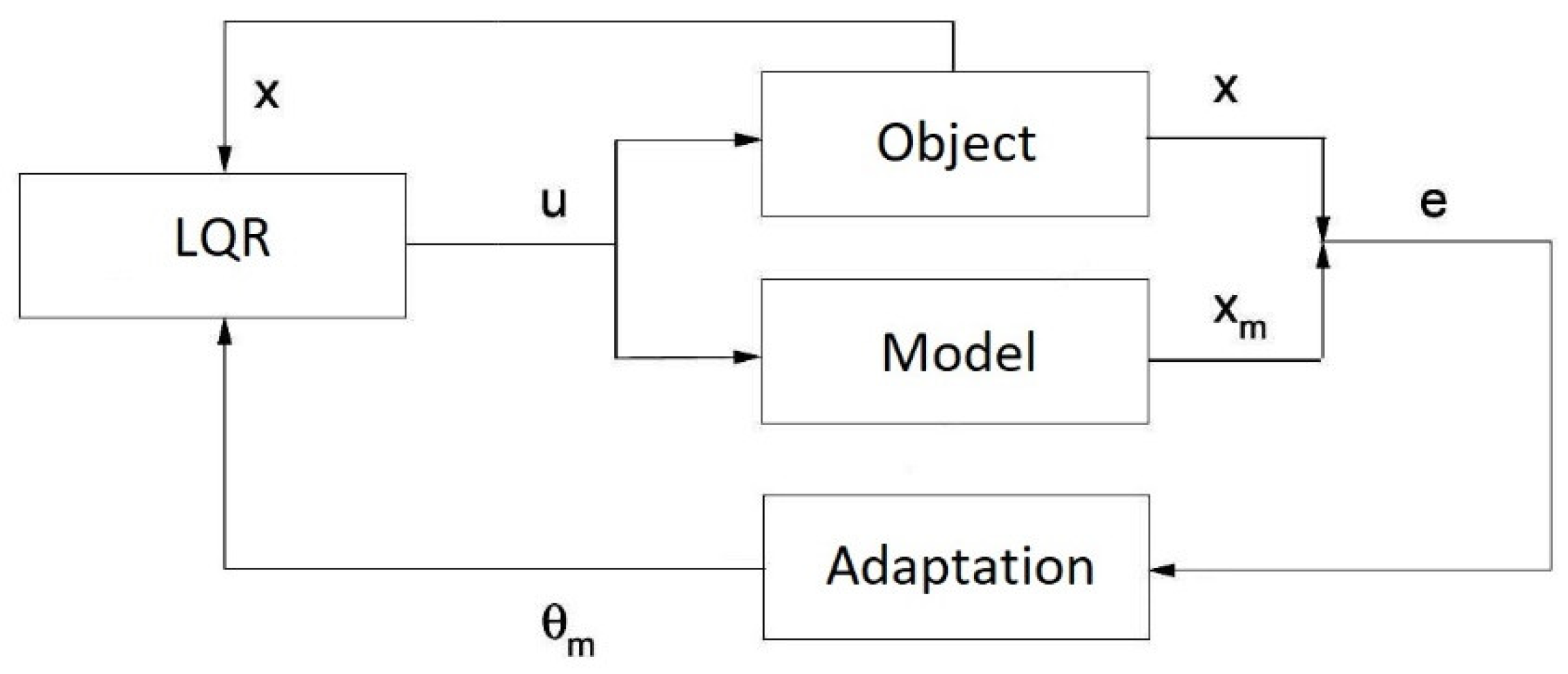
The idea of the method used for solving the formulated problem can be described as follows. Based on the error stemming from the actual state x, and the state estimated from the model $x_m$, unknown elements of the matrices A and B are identified. Then, based on the results, the LQR regulator (4) is tuned (Figure 1).

The continuous version of the least squares method was used to identify the looked-for elements of the matrices A and B. The estimation is based on the minimization of the integral from the squared standard error ($e=x-x_m$):

$$\underset{{\mathsf{\theta }}_m}{{\displaystyle \min }}{\displaystyle \underset{0}{\overset{t}{\int }}||e|{|}^{2}d\tau }$$

(7)

where the Euclidean standard is described by the formula:

$$||e||=\sqrt{e^{T}e}=\sqrt{{\displaystyle \sum _{i=1}^n{e}_i{}^2}}$$

(8)

assuming there exists a linear relationship:

$$x_m={\mathsf{\Phi }}^T{\mathsf{\theta }}_m$$

(9)

where

${\mathsf{\theta }}_m$—k-dimensional vector of estimates of identified elements of matrices A and B (its coordinates are part of the matrix $A_m$ and $B_m$);

$\mathsf{\Phi }$—measurement matrix, regressor (with dimensions $k\times n$).

The Equation (7) can be written in the form of:

$$\underset{{\mathsf{\theta }}_m}{{\displaystyle \min }}{\displaystyle \underset{0}{\overset{t}{\int }}||x-{\mathsf{\Phi }}^T{\mathsf{\theta }}_m|{|}^{2}d\tau }$$

(10)

Therefore, vector ${\mathsf{\theta }}_m$ is determined from the relationship (derived by comparing the derivative versus ${\mathsf{\theta }}_m$ from Equation (10) to zero):

$${\displaystyle \underset{0}{\overset{t}{\int }}\mathsf{\Phi }\left(x-{\mathsf{\Phi }}^T{\mathsf{\theta }}_m\right)d\tau }=0$$

(11)

which after transformation (provided that for a set t the vector ${\mathsf{\theta }}_m$ is treated as a constant) and has this form:

$$K{\mathsf{\theta }}_m={\displaystyle \underset{0}{\overset{t}{\int }}\mathsf{\Phi }xd\tau }$$

(12)

where

$K={\displaystyle \underset{0}{\overset{t}{\int }}\mathsf{\Phi }{\mathsf{\Phi }}^{T}d\tau }$—a regular matrix (where the initial condition is a positive definite matrix) with $k\times k$ dimensions.

Differentiating Equation (12) with respect to time we obtain:

$$\dot{K}{\mathsf{\theta }}_m+K{\dot{\mathsf{\theta }}}_m=\mathsf{\Phi }x$$

(13)

where after substitution:

$$\dot{K}=\mathsf{\Phi }{\mathsf{\Phi }}^T$$

(14)

and simple transformations we get a formula for the identification of model parameters:

$${\mathsf{\theta }}_m={\displaystyle \underset{0}{\overset{t}{\int }}{K}^{-1}\mathsf{\Phi }ed\tau }$$

(15)

By means of the model parameters identified using the Formula (15) we can determine the LQR (4) gain, which will assure the system adaptation.

3. Stability of the Adaptive Control System

The stability of the proposed system will be proved below. The system (1) with feedback (4) is stable [20], and therefore for a symmetric and positive definite matrix $Q$, the matrix ${\left(A+B{R}_u{}^{-1}{B}^{T}P\right)}^{T}Q+Q\left(A+B{R}_u{}^{-1}{B}^{T}P\right)$ is non-positive definite and symmetric. This results from the Lapunov equation for a stable dynamic linear system (in the Lapunov sense).

Taking into account the feedback in Equation (6), it will be transformed to this form:

$${\dot{x}}_m=A_m{x}_m+B_{m}u=\left(A_m+B_m{R}_u{}^{-1}{B}_m{}^T{P}_m\right)x_m$$

(16)

where

$A_m,B_m$—matrices $A,B$ identified by means of Formula (15);

$P_m$—solution of the Equation (5) for $A=A_m$, $B=B_m$.

The derivative of error e with respect to time can be written as:

$$\dot{e}=\dot{x}-\frac{x_m}{x}\dot{x}+\frac{x_m}{x}\dot{x}-{\dot{x}}_m$$

(17)

which after substitution of the Equations (1), (4), (16) will take the form:

$$\dot{e}=\left(A+B{R}_u{}^{-1}{B}^{T}P\right)e+\left(A-A_m+B{R}_u{}^{-1}{B}^{T}P-B_m{R}_u{}^{-1}{B}_m{}^T{P}_m\right)x_m$$

(18)

For clarity, the second term of the sum in Equation (18) will be omitted (as being limited) which yields:

$$\dot{e}=\left(A+B{R}_u{}^{-1}{B}^{T}P\right)e$$

(19)

Let the positive definite quadratic form:

$$V\left(e\right)=e^{T}Qe$$

(20)

be the Lapunov function of the system in question. The time derivative of the function has this form:

$$\dot{V}\left(e\right)={\dot{e}}^{T}Qe+e^{T}Q\dot{e}$$

(21)

and by substituting the relationship (19) we get:

$$\dot{V}\left(e\right)=e^T\left({\left(A+B{R}_u{}^{-1}{B}^{T}P\right)}^{T}Q+Q\left(A+B{R}_u{}^{-1}{B}^{T}P\right)\right)e$$

(22)

Therefore, because the matrix ${\left(A+B{R}_u{}^{-1}{B}^{T}P\right)}^{T}Q+Q\left(A+B{R}_u{}^{-1}{B}^{T}P\right)$ is non-positive definite, this relation exists:

$$\dot{V}\left(e\right)\le 0$$

(23)

which proves the stability of the adaptive control system herein considered. If we also take into account the second term of Equation (18), to obtain the system stability we have to use the sliding mode control [21], which consists of adding a properly selected signal to the control, which will guarantee the inequality (23) to take place. This is successfully done when we know the vector’s $\left(A-A_m+B{R}_u{}^{-1}{B}^{T}P-B_m{R}_u{}^{-1}{B}_m{}^T{P}_m\right)x_m$ component constraints and we additionally assume that only one element of the matrix $B$ is non-zero (then $B$ is an n-element vector, while the control is a scalar). In such a case, the control signal in Equation (16) will be:

$$u=R_u{}^{-1}{B}_m{}^T{P}_m{x}_m+\frac{n\cdot \underset{1\le i\le n}{\max }\left\{o_i\right\}\cdot \underset{1\le i\le n}{\max }\left\{|{\left(Qe\right)}_i|\right\}}{{\left(b_m\right)}_j{\left(Qe\right)}_j}$$

(24)

where

$o_i$—known upper i-th vector $|(A-A_m+B{R}_u{}^{-1}{B}^{T}P-B_m{R}_u{}^{-1}{B}_m{}^T{P}_m)x_m|$ element constraint $\left(1\le i\le n\right)$;

${\left(Qe\right)}_i$—i-th vector $Qe$ element $\left(1\le i\le n\right)$;

${\left(b_m\right)}_j$—j-th vector $B_m$ element, where j means the non-zero vector $B$ element numeral.

It will be noted in further considerations that inequality (23) will occur, which has been shown.

4. Trajectory Autopilot

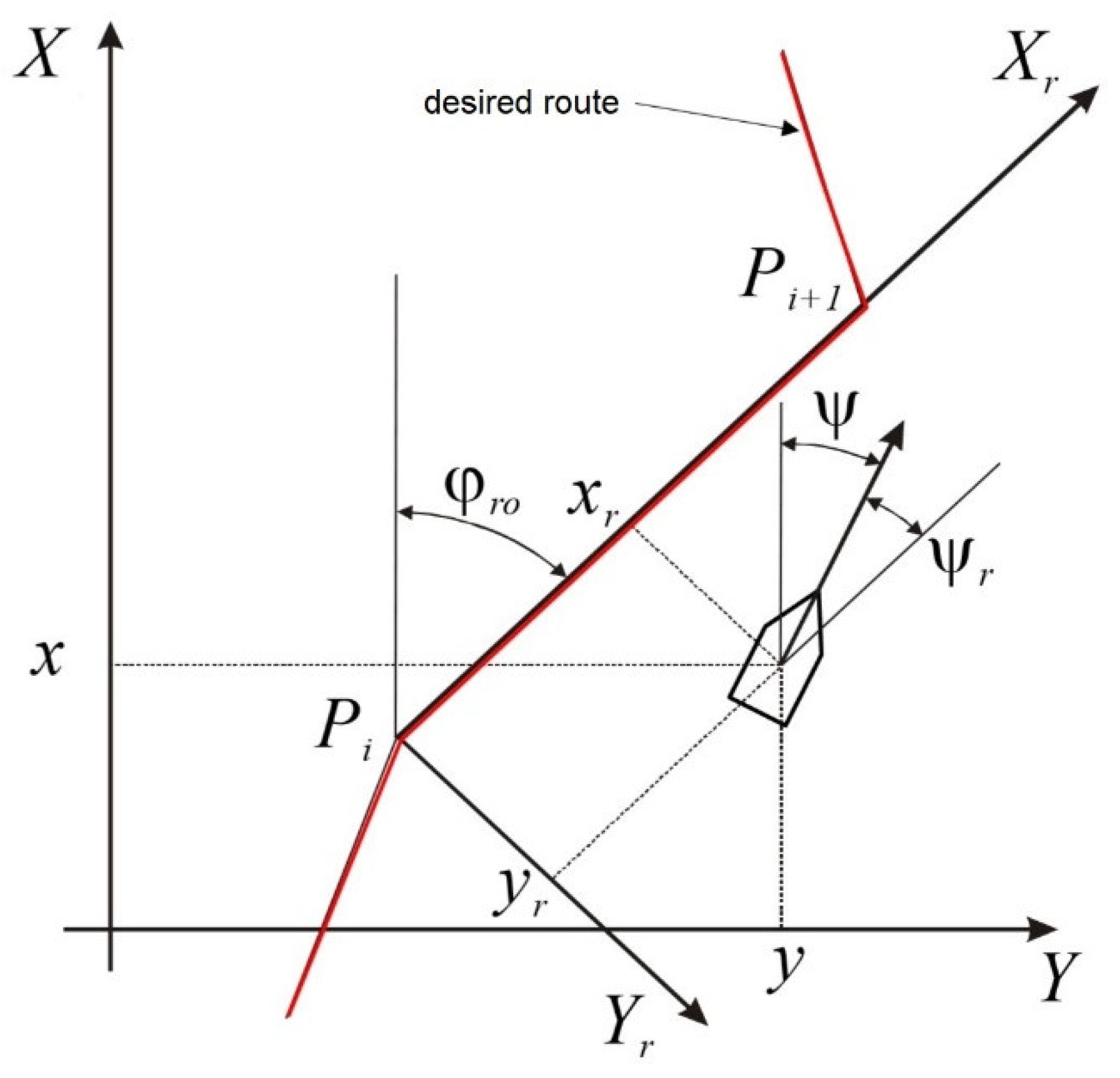
The track along which the ship should be steered is defined as a broken line defined by n preset waypoints $P_1\left(x_1,y_1\right)$, $P_2\left(x_2,y_2\right)$, …, $P_i\left(x_i,y_i\right)$, …, $P_n\left(x_n,y_n\right)$ $\left(1\le i\le n\right)$. To formalize the problem of keeping track of the ship, two reference systems will be introduced (Figure 2):

• global, stationary to the ground $\left(X,Y\right)$;
• relative (mobile) $\left(X_r,Y_r\right)$, with the origin located in the latest reached waypoint $P_i\left(x_i,y_i\right)$, and the vertical axis along the section $P_i{P}_{i+1}$ (${\varphi }_{ro}$—the angle of the relative reference system rotation).

Figure 2 also depicts the ship’s gyrocompass course $\psi$ and the relative course ${\psi }_r$. The relative position of the ship, and its relative course are obtained by transformation:

$$\left[\begin{array}{c}{x}_r\\ y_r\\ {\psi }_r\end{array}\right]=\left[\begin{array}{ccc}\cos {\varphi }_{ro}& \sin {\varphi }_{ro}& 0\\ -\sin {\varphi }_{ro}& \cos {\varphi }_{ro}& 0\\ 0& 0& 1\end{array}\right]\left[\begin{array}{c}x-x_i\\ y-y_i\\ \psi -{\varphi }_{ro}\end{array}\right]$$

(25)

which defines the subsequent displacements and rotations of the global reference system depending on the current track leg. The system rotation angle is defined as follows:

$${\varphi }_{ro}=\{\begin{array}{ccc}arctg\left(\frac{y_{i+1}-y_i}{x_{i+1}-x_i}\right)& gdy& x_i\ne x_{i+1}\\ \pi /2& gdy& x_i=x_{i+1}\wedge y_i<y_{i+1}\\ -\pi /2& gdy& x_i=x_{i+1}\wedge y_i>y_{i+1}\end{array}$$

(26)

The rotation of the system is made after the condition is met:

$$|P_i{P}_{i+1}|-x_r<R$$

(27)

where

$R$—radius reaching the waypoint, a positive value determined arbitrarily.

Let the model describing the ship’s movement dynamics be a Nomoto model [22]. Then, to be consistent with the form (1), the following denotations are made:

$$A=\left[\begin{array}{ccc}0& u& 0\\ 0& 0& 1\\ 0& 0& -a\end{array}\right],B=\left[\begin{array}{c}0\\ 0\\ c\end{array}\right],x=\left[\begin{array}{c}{y}_r\\ {\psi }_r\\ r\end{array}\right],u=\left[\delta \right]$$

(28)

where

$a,c$—coefficients determined from model tests (different for different types of vessels);

$u$—longitudinal speed of the ship (as an approximation the actual speed can be accepted);

$r$—rate of turn;

$\delta$—rudder angle.

The control quality, when the track for the ship to follow has been set, is most commonly expressed by the indicator:

$$J\left(\delta \right)={\displaystyle \underset{0}{\overset{\infty }{\int }}\left({\lambda }_y{\left(y_r\right)}^2+{\lambda }_{\psi }{\left({\psi }_r\right)}^2+{\lambda }_{\delta }{\delta }^2\right)dt}$$

(29)

where ${\lambda }_y,{\lambda }_{\psi },{\lambda }_{\delta }$—coefficients greater than zero, arbitrarily determined, which, after introducing the matrices:

$$R_x=\left[\begin{array}{ccc}{\lambda }_y& 0& 0\\ 0& {\lambda }_{\psi }& 0\\ 0& 0& 0\end{array}\right],R_u=\left[{\lambda }_{\delta }\right]$$

(30)

will take the form (3).

If we assume that the coefficients a, c are known and fixed (and not time-dependent), the optimal control of track-keeping can be found from the relation (4).

Let the equation describing the object (ship) be the Nomoto model, but not taking into account the deviation from the course as a component of the state:

$$\dot{r}=-ar+c\delta$$

(31)

and a_m, c_m (established arbitrarily) will be the estimated model parameters. To use the identification Formula (15), first the Laplace transformation will be applied (for initial zero conditions) in Equation (31), then two filtered signals will be substituted:

$$\begin{array}{c}{r}_f\left(s\right)=\frac{1}{1+s}r\left(s\right)\\ {\delta }_f\left(s\right)=\frac{1}{1+s}\delta \left(s\right)\end{array}$$

(32)

after transformation and returning to the time domain, we obtain:

$$r_m=\left(1-a_m\right)r_f+c_m{\delta }_f$$

(33)

By introducing the denotations:

$$\mathsf{\Phi }=\left[\begin{array}{c}{r}_f\\ {\delta }_f\end{array}\right],{\mathsf{\theta }}_m=\left[\begin{array}{c}1-a_m\\ c_m\end{array}\right],x=\left[r\right]$$

(34)

we get a conformity of (33) with the form (15). Formula (15) can now be used for the continuous identification of the parameters of the Nomoto model. With the identified vector ${\mathsf{\theta }}_m$ of the Nomoto model parameters, the optimal control of track-keeping is determined from relation (4).

It should be noted that the control quality of the presented trajectory autopilot can depend on the parameters ${\lambda }_y,{\lambda }_{\psi },{\lambda }_{\delta },R$ and the initial estimates a, c. The assumption here is that they are adopted arbitrarily. The automatic selection of these parameters goes beyond the framework of this work and will be examined in the future.

5. Calculation Experiments

The experiments were made in the Matlab/Simulink environment. A de Witt–Oppe model [23] was used as an object (vessel), incorporating the dynamics of the steering gear [22]:

$$\begin{array}{l}{\dot{x}}_1=x_5\cos x_3-x_6\sin x_3\hfill \\ {\dot{x}}_2=x_5\sin x_3+x_6\cos x_3\hfill \\ {\dot{x}}_3=x_4\hfill \\ {\dot{x}}_4=-a_1{x}_4-a_2{x}_4{}^3+a_{3}u\hfill \\ {\dot{x}}_5=-f{x}_5-W{x}_4{}^2+S\hfill \\ x_6=-r_1{x}_4-r_3{x}_4{}^3\hfill \\ \dot{u}=u_z-u\hfill \\ |u_z|\le u_{\max }\hfill \\ |\dot{u}|\le {\dot{u}}_{\max }\hfill \end{array}$$

(35)

where

$(x_1,x_2)=(x,y)$—Cartesian coordinates (ship’s position),

$x_3=\psi$—deviation from the course,

$x_4=r$—angular velocity,

$x_5$—longitudinal speed,

$x_6$—lateral speed,

$u=\delta$—rudder angle,

$u_z={\delta }_z$—preset rudder angle,

${\delta }_{\max }$—maximum rudder angle,

${\dot{\delta }}_{\max }$—maximum rate of turn of the rudder,

S—propeller thrust,

$a_1,a_2,a_3,f,W,r_1,r_3$—coefficients determined from model tests (different for different types of vessels).

The ship movement parameters assumed here are those of a ship of mariner class, such as the m.s. Compass Island [23]: a₁ = 0.018(1/s), a₂ = 37.2(s/rad²), a₃ = 0.001(1/s²), f = 0.014(1/s), w = 124(m/rad²), s = 0.11(m/s²), r₁ = −69.5(m/rad), r₃ = 0(m·s²/rad³). The selected ship has the following characteristics: gross registered tons 9214 (t), 13498 DWT (Dead Weight Tonnage) (t), single screw, length 172 (m), maximum draft 8 (m), maximum speed 20 (knots), maximum (minimum) angular velocity r_max = 0.0191(rad/s) (r_min = −0.0191(rad/s)), maximum (minimum) rudder angle δ_max = 0.6(rad) (δ_min = −0.6(rad)), maximum (minimum) rate of turn of the rudder ${\dot{\delta }}_{\max }$ = 0.066(rad/s) (${\dot{\delta }}_{\min }$ = −0.066(rad/s)).

In order to take account of disturbances, the simulations included a signal characteristic of wind-induced sea waves (the wind direction conforms with the direction of the Y axis) [22].

The established initial parameters of the simulation were as follows: angular velocity r = 0 (rad/s), deviation from the course ψ = 0 (rad), rudder angle δ = 0 (rad), ship’s speed v = 7.7 (m/s), and ship’s position $\left(0,-500\right)\left(\mathrm{m}\right)$. The time span of the simulation was determined at 1000 (s).

The track to be followed by the ship was determined by setting the waypoints $P_1\left(0,0\right)$, $P_2\left(3000,0\right)$, $P_3\left(3000,1000\right)$, and $P_4\left(10,000,1000\right)\left(m\right)$.

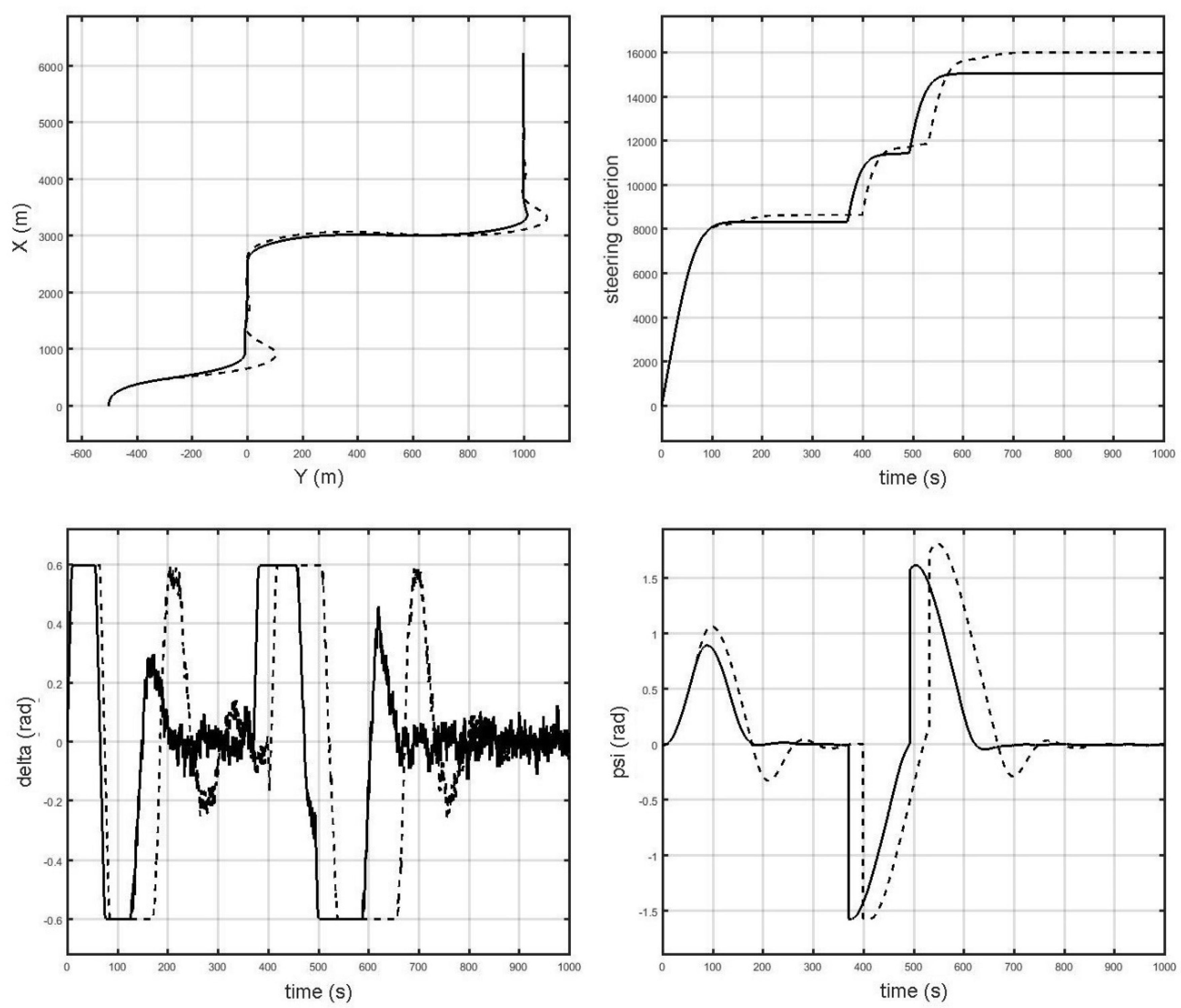
The calculation experiments were conducted to compare the performance of the proposed adaptive system and the LQR regulator without the identification of the model parameters. The values ${\lambda }_y=1/2000$, ${\lambda }_{\psi }=1$, ${\lambda }_{\delta }=5$, R = 500 (m) were arbitrarily accepted as the LQR regulator parameters. Figure 3 shows an example simulation result for the case where the initial estimates of the Nomoto model parameters assumed the values a₀ = 0.02 (1/s) and c₀ = 0.002 (1/s²) (nominal values a = 0.018(1/s), c = 0.001(1/ s²)). Preliminary estimates of the Nomoto model parameters were used for the determination of the LQR regulator’s gain and as input data for the adaptive algorithm. The charts illustrate, respectively, the simulation results: ship movement trajectory, control quality indicator, rudder angle, and deviation from the course. It can be observed that both the control by the proposed method and by LQR lead to the ship correctly stabilizing its position relative to the planned track. However, the proposed method had a significantly higher control quality. This applies to the value of the control quality indicator (lower for the proposed method) and to oscillations and overshoots (lower in the proposed method). It should be noted that the oscillation of the presented system (the lower left chart) can depend on the parameters ${\lambda }_y,{\lambda }_{\psi },{\lambda }_{\delta }$, which is interpreted as a compromise between the deviation from the route and the rudder angle (steering gear load). The automatic selection of these parameters goes beyond the framework of this work and will be examined in the future.

The situation presented in the experiment is typical of this kind of research. In all cases considered, the value of the quality indicator for the ship controlled by the proposed adaptive system was lower than in the case of the LQR regulator without the identification of the model parameters. The method led to a reduction of the control quality indicator value to 15%, depending on the assumed initial estimates of the Nomoto model parameters.

6. Conclusions

The article presented an adaptive control system for keeping track of a ship as an element of an intelligent system applicable in modern marine navigation [24,25,26,27,28,29,30,31,32,33,34,35]. An optimal LQR regulator with a symmetric indicator of control quality was adopted as the control algorithm. The model identification was based on the continuous version of the least squares method.

The results of calculation experiments clearly confirmed the high quality of control of the proposed adaptive system. This refers to the minimization of the control criterion values as well as the reduction of oscillation and overshoot. In all examined cases, the control quality of the proposed system was higher than that of the LQR regulator without the identification of the model parameters.

The proposed solution effectively stabilized the ship’s trajectory relative to the desired track, and the whole process ran in the online mode. The simplicity of the method and the lack of application limitations are relevant for the implementation of the developed system on vessels. The proposed adaptive algorithm for automatic track-keeping by a ship is a functional solution, characterized by high control quality that can be effectively implemented in navigational systems.