Article

A Numerical Solution of Fractional Lienard’s Equation by Using the Residual Power Series Method

Department of Mathematical Sciences, United Arab Emirates University, Al-Ain 15551, United Arab Emirates
Mathematics 2018, 6(1), 1; https://doi.org/10.3390/math6010001
Submission received: 1 October 2017 / Revised: 19 November 2017 / Accepted: 21 November 2017 / Published: 22 December 2017
(This article belongs to the Special Issue Advances in Differential and Difference Equations with Applications)

Abstract

:
In this paper, we investigate a numerical solution of Lienard’s equation. The residual power series (RPS) method is implemented to find an approximate solution to this problem. The proposed method is a combination of the fractional Taylor series and the residual functions. Numerical and theoretical results are presented.

1. Introduction

The ordinary Lienard’s equation is given by:
y ( x ) + f ( y ) y ( x ) + g ( y ) = r ( x ) .
Different choices of f , g , and r will produce different models. For example, if f ( y ) y ( x ) is the damping force, g ( y ) is the restoring force, and r ( x ) is the external force, we get the damped pendulum equation. However, if we choose f ( y ) = ϵ ( y 2 1 ) , g ( y ) = y , and r ( x ) = 0 , we get a nonlinear model of electronic oscillation, see [1,2].
Several researchers have studied the exact solution of special cases of Equation (1). For example, Feng [3] investigated the exact solution of:
y ( x ) + a y ( x ) + b y 3 ( x ) + c y 5 ( x ) = 0 .
He found that one of the solutions to Equation (2) is given by:
y ( x ) = 2 a b ( 1 + tan ( a x )
when b 2 4 4 a c 3 = 0 , b > 0 , and a < 0 . Several methods are used to investigate the solution of nonlinear equation such as the homotopy analysis method (HAM), Adomian decomposition method, and variational method [4,5,6,7,8,9,10,11,12]. Equation (2) was studied by many researchers, notably Kong [13], Matinfar et al. [14,15], and others. In this paper, we generalize Equation (2) to the fractional case. It is not an easy task to solve highly nonlinear differential equations of fractional order. Many of the researchers tried to solve nonlinear equations by using different techniques. For example, Liao studied an analytical method termed as the HAM [9,10,11] to examine nonlinear problems. Furthermore, the HAM is used by many researchers to solve various types of nonlinear problems such as fractional Black–Scholes equation [12], natural convective heat and mass transfer in a steady 2-D MHD fluid flow over a stretching vertical surface via porous media [16], micropolar flow in a porous channel in the presence of mass injection [17], etc. The standard classical analytic schemes require more computational time and computer memory. Some researchers combine analytical techniques with Laplace transform to study nonlinear problems such as a class of nonlinear differential equations [18], the nonlinear boundary value problem on a semi infinite domain [19], the fractional convection–diffusion equation [20], the fractional Keller–Segel model [21], fractional coupled Burgers equations [16], and the synthesis of FO-PID controllers [22]. In this paper, we consider the following class of fractional Lienard’s equation of the form:
D 2 α y ( x ) + a y ( x ) + b y 3 ( x ) + c y 5 ( x ) = 0 , x > 0 , 1 2 < α 1 ,
subject to:
y ( 0 ) = y 0 , D α y ( 0 ) = y 1
where a , b , c , y 0 , and y 1 are constants. The derivative in Equation (4) is in the Caputo sense. The Caputo derivative is defined as follows; see [23,24].
Definition 1.
Let n be the smallest integer greater than or equal to α . The Caputo fractional derivative of order α > 0 is defined as:
D α y ( x ) = 1 Γ ( n α ) 0 x ( x t ) n α 1 y ( n ) ( t ) d t , n 1 < α < n , y ( n ) ( x ) , α = n N . .
The power rule of the Caputo derivative is given as follows.
Theorem 1.
The Caputo fractional derivative of the power function is given by:
D α x p = Γ ( p + 1 ) Γ ( p α + 1 ) x p α , n 1 < α < n , p > n 1 , p R , 0 , n 1 < α < n , p n 1 , p N .
We implement the residual power series (RPS) method [13,25,26,27] to solve Equation (4). We start by the following definition and some theorems related to the RPS, [13,27].
Definition 2.
A power series expansion of the form:
m = 0 c m ( x x 0 ) m α = c 0 + c 1 ( x x 0 ) α + c 2 ( x x 0 ) 2 α +
where 0 n 1 < α n , x x 0 , is called fractional power series FPS about x = x 0 .
Theorem 2.
Suppose that f has a RPS representation at x = x 0 of the form:
f ( x ) = m = 0 c m ( x x 0 ) m α , x 0 x < x 0 + R ,
where R is the radius of convergence. If D m α f ( x ) , m = 0 , 1 , 2 , are continuous on ( x 0 , x 0 + R ) , then c m = D m α f ( x 0 ) Γ ( 1 + m α ) .

2. The Residual Power Series Method for Fractional Lienard’s Equation

Write the solution of Equation (4) as a fractional power series of the form:
y ( x ) = n = 0 y n x n α Γ ( 1 + n α ) .
Using the initial conditions in Equation (5), we approximate y ( x ) in Equation (6) by:
y k ( x ) = y 0 + y 1 x α Γ ( 1 + α ) + n = 2 k y n x n α Γ ( 1 + n α ) , k = 2 , 3 ,
where y 1 ( x ) = y 0 + y 1 x α Γ ( 1 + α ) is considered as the first RPS approximate solution of y ( x ) . To find the values of the RPS-coefficients y n , n = 2 , 3 , 4 , , we solve the equation:
D ( n 2 ) α R e s n ( 0 ) = 0 , n = 2 , 3 , 4 ,
where R e s k ( x ) is the kth residual function [13,27] and it is defined by:
R e s k ( x ) = D 2 α y k ( x ) + a y k ( x ) + b y k 3 ( x ) + c y k 5 ( x ) .
To find y 2 in Equation (7), we substitute the second RPS approximate solution y 2 ( x ) = y 0 + y 1 x α Γ ( 1 + α ) + y 2 x 2 α Γ ( 1 + 2 α ) into:
R e s 2 ( x ) = D 2 α y 2 ( x ) + a y 2 ( x ) + b y 2 3 ( x ) + c y 2 5 ( x )   = y 2 + a y 0 + y 1 x α Γ ( 1 + α ) + y 2 x 2 α Γ ( 1 + 2 α )     + b y 0 + y 1 x α Γ ( 1 + α ) + y 2 x 2 α Γ ( 1 + 2 α ) 3     + c y 0 + y 1 x α Γ ( 1 + α ) + y 2 x 2 α Γ ( 1 + 2 α ) 5 .
Then, we solve R e s 2 ( 0 ) = 0 to get:
y 2 = a y 0 + b y 0 3 + c y 0 5 .
To find y 3 in Equation (7), we substitute the third RPS approximate solution y 3 ( x ) = y 0 + y 1 x α Γ ( 1 + α ) + y 2 x 2 α Γ ( 1 + 2 α ) + y 3 x 3 α Γ ( 1 + 3 α ) into:
R e s 3 ( x ) = D 2 α y 3 ( x ) + a y 3 ( x ) + b y 3 3 ( x ) + c y 3 5 ( x )   = y 2 + y 3 x α Γ ( 1 + α ) + a y 0 + y 1 x α Γ ( 1 + α ) + y 2 x 2 α Γ ( 1 + 2 α ) + y 3 x 3 α Γ ( 1 + 3 α )     + b y 0 + y 1 x α Γ ( 1 + α ) + y 2 x 2 α Γ ( 1 + 2 α ) + y 3 x 3 α Γ ( 1 + 3 α ) 3     + c y 0 + y 1 x α Γ ( 1 + α ) + y 2 x 2 α Γ ( 1 + 2 α ) + y 3 x 3 α Γ ( 1 + 3 α ) 5 .
Then, we solve D α R e s 3 ( 0 ) = 0 to get:
y 3 = a y 1 + 3 b y 0 2 y 1 + 5 c y 0 4 y 1 .
In general, to find y k ( x ) , we substitute the k t h RPS approximate solution y k ( x ) into:
R e s k ( x ) = D 2 α y k ( x ) + a y k ( x ) + b y k 3 ( x ) + c y k 5 ( x ) .
Then, we solve D t ( k 2 ) α R e s k ( 0 ) = 0 to get:
y k = a y k 2 + b i = 0 k 2 j = 0 k 2 i y i y j y k 2 i j Γ ( 1 + ( k 2 ) α ) Γ ( 1 + i α ) Γ ( 1 + j α ) Γ ( 1 + ( k 2 i j ) α ) + c i = 0 k 2 j = 0 k 2 i l = 0 k 2 i j m = 0 k 2 i j l y i y j y l y m y k 2 i j l m Γ ( 1 + ( k 2 ) α ) Γ ( 1 + i α ) Γ ( 1 + j α ) Γ ( 1 + l α ) Γ ( 1 + m α ) Γ ( 1 + ( k 2 i j l m ) α ) .

3. Convergence Analysis

In this section, we prove the convergence of the proposed method. We start by the following lemma.
Lemma 1.
The classical power series n = 0 y n x n , < x < , has a radius of convergence R if and only if the fractional power series n = 0 y n x α n , x 0 , has a radius of convergence R 1 α .
Proof. 
See [28].
Theorem 3.
The fractional power series:
y ( x ) = n = 0 y n x n α Γ ( 1 + n α )
where the coefficients are defined in Equation (15) has a positive radius of convergence.
Proof. 
From Equation (15), one can see that:
y k Γ ( 1 + k α ) A y k 2 + B i = 0 k 2 j = 0 k 2 i y i y j y k 2 i j + C i = 0 k 2 j = 0 k 2 i l = 0 k 2 i j m = 0 k 2 i j l y i y j y l y m y k 2 i j l m
where:
A = a Γ ( 1 + k α ) , B = M a x 0 j k 2 i 0 i k 2 k Γ ( 1 + ( k 2 ) α ) Γ ( 1 + i α ) Γ ( 1 + j α ) Γ ( 1 + ( k 2 i j ) α ) Γ ( 1 + k α ) b , C = M a x 0 m k 2 i j l 0 l k 2 i j 0 j k 2 i 0 i k 2 k Γ ( 1 + ( k 2 ) α ) ρ i , j , k , l , m c , ρ i , j , k , l , m = Γ ( 1 + i α ) Γ ( 1 + j α ) Γ ( 1 + l α ) Γ ( 1 + m α ) Γ ( 1 + ( k 2 i j l m ) α ) Γ ( 1 + k α ) .
Let:
f ( x ) = k = 0 a k x k
where a 0 = y 0 , a 1 = y 1 Γ ( 1 + α ) , and
a k = A a k 2 + B i = 0 k 2 j = 0 k 2 i a i a j a k 2 i j + C i = 0 k 2 j = 0 k 2 i l = 0 k 2 i j m = 0 i k 2 i j l a i a j a l a m a k 2 i j l m
for k = 2 , 3 , Then,
ω = f ( x ) = a 0 + a 1 x + x 2 k = 0 a k + 2 x k   = a 0 + a 1 x + x 2 A k = 0 a k x k + B k = 0 i = 0 k j = 0 k i a i a j a k i j x k + C k = 0 i = 0 k j = 0 k i l = 0 k i j m = 0 i k i j l a i a j a l a m a k i j l m x k .
Let:
H ( x , ω ) = ω a 0 a 1 x x 2 A ω + B ω 3 + C ω 5 .
It is easy to see that H ( x , ω ) is an analytic function in the ( x , ω ) plane and
H ( 0 , a 0 ) = 0 , H ω ( 0 , a 0 ) = 1 0 .
By implicit function theorem [29], f ( x ) is analytic function in a neighborhood of the point ( 0 , a 0 ) of the ( x , ω ) plane with a positive radius of convergence. Thus, the series in Equation (6) is convergent by Lemma 1. ☐

4. Numerical Results

In this section, we present four examples to show the efficiency of the proposed approach. Comparison with the exact solution presented in Equation (3) is reported in Table 1, Table 2, Table 3 and Table 4 for different choices of a , b , and c with α = 1 . Let:
e r r o r ( x ) = y e x a c t ( x ) y 5 ( x ) , x 0 .
In these two examples, we use k = 3 . Then,
y 2 = a y 0 + b y 0 3 + c y 0 5 , y 3 = a y 1 + 3 b y 0 2 y 1 + 5 c y 0 4 y 1 .
Example 1.
Consider the following class of fractional differential equation:
D 2 α y ( x ) y ( x ) + 3 y 3 ( x ) 27 16 y 5 ( x ) = 0 , 1 2 < α 1 ,
subject to:
y ( 0 ) = y 0 = 2 3 , D α y ( 0 ) = y 1 = 1 6 .
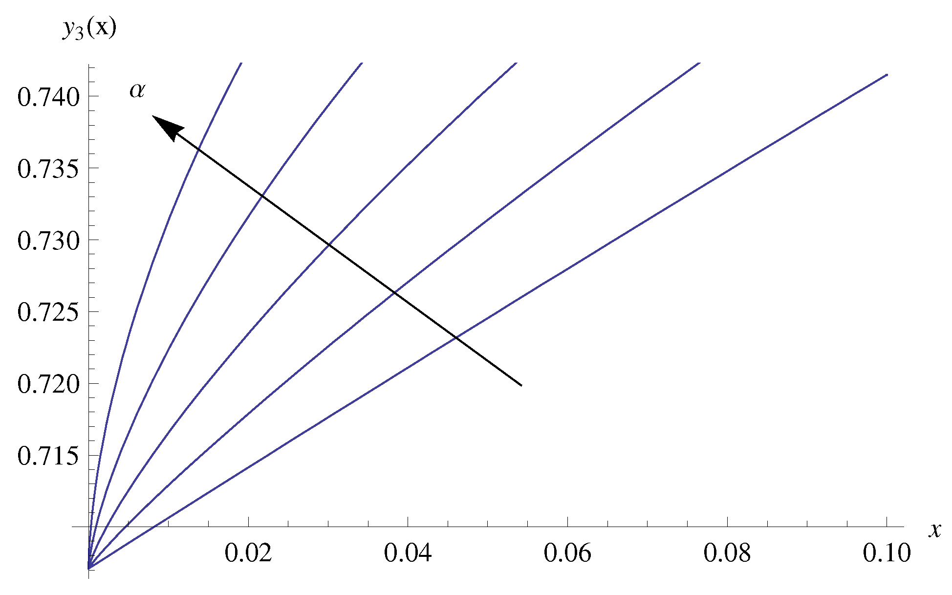
Then, the error, when α = 1 , is reported in Table 1. Figure 1 shows the effect of α on the solution for α = 0 . 6 , 0 . 7 , 0 . 8 , 0 . 9 , 1 .
Example 2.
Consider the following class of fractional differential equation:
D 2 α y ( x ) y ( x ) + 4 y 3 ( x ) 3 y 5 ( x ) = 0 , 1 2 < α 1 ,
subject to:
y ( 0 ) = y 0 = 1 2 , D α y ( 0 ) = y 1 = 1 8 .
Then, the error, when α = 1 , is reported in Table 2. Figure 2 shows the effect of α on the solution for α = 0 . 6 , 0 . 7 , 0 . 8 , 0 . 9 , 1 .
Example 3.
Consider the following class of fractional differential equation:
D 2 α y ( x ) y ( x ) + 2 y 3 ( x ) 3 4 y 5 ( x ) = 0 , 1 2 < α 1 ,
subject to:
y ( 0 ) = y 0 = 1 , D α y ( 0 ) = y 1 = 1 .
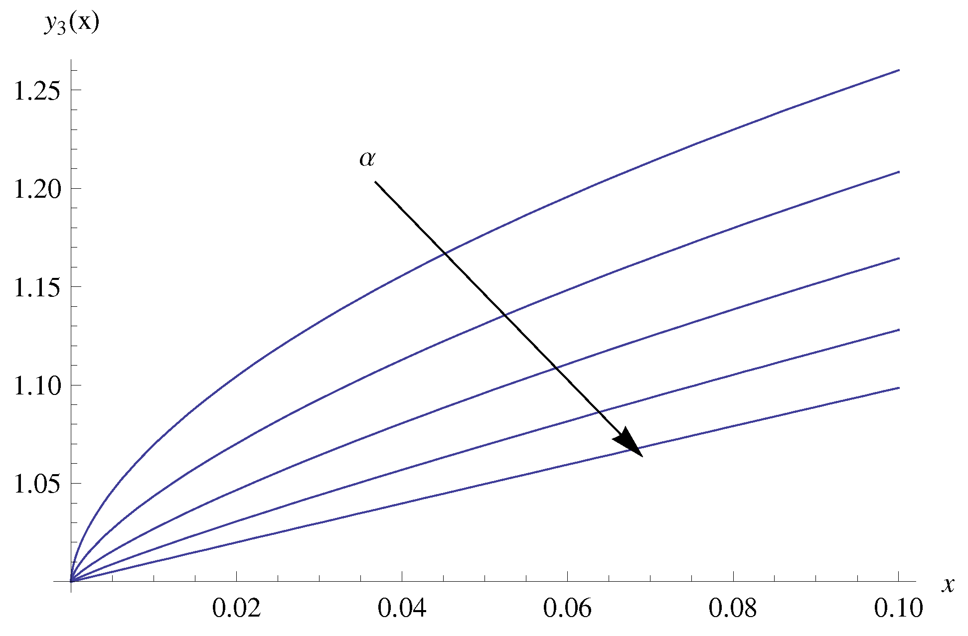
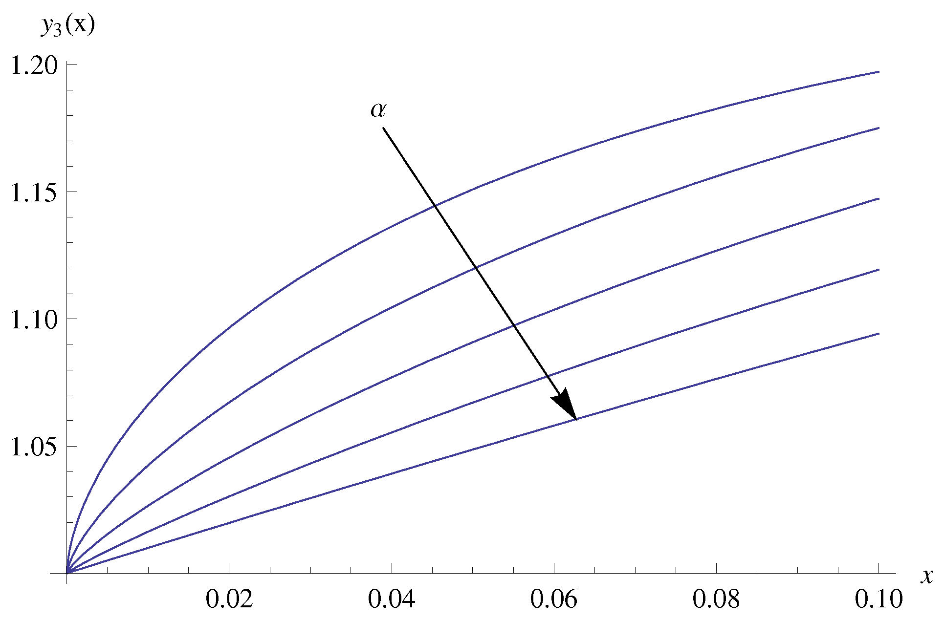
Then, the error, when α = 1 , is reported in Table 3. Figure 3 shows the effect of α on the solution for α = 0 . 6 , 0 . 7 , 0 . 8 , 0 . 9 , 1 .
Example 4.
Consider the following class of fractional differential equation:
D 2 α y ( x ) 4 y ( x ) + 8 y 3 ( x ) 3 y 5 ( x ) = 0 , 1 2 < α 1 ,
subject to:
y ( 0 ) = y 0 = 1 , D α y ( 0 ) = y 1 = 1 .
Then, the error, when α = 1 , is reported in Table 4. Figure 4 shows the effect of α on the solution for α = 0 . 6 , 0 . 7 , 0 . 8 , 0 . 9 , 1 .

5. Conclusions

In this paper, we have investigated the analytical solution of Lienard’s equation based on the RPS method. Convergence of the proposed infinite series is presented. Four examples of our numerical results are presented. Comparison with the exact solution when α = 1 is reported in Table 1, Table 2, Table 3 and Table 4. From Table 1, Table 2, Table 3 and Table 4, we see that the approximate solute is close to the exact solution with four terms only. From Figure 1 and Figure 2, we see that as α is increasing, the approximate solution is increasing while from Figure 3 and Figure 4, we see that as α is increasing, the approximate solution is decreasing. We see that this approach is cheap compared with other methods and we obtain accurate results using four terms only. A reasonably accurate solution can be achieved with only a few terms. Moreover, the proposed method can be applied to several nonlinear models in science and engineering.

Acknowledgments

In addition, The authors would like to express their appreciation for the valuable comments of the reviewers.

Conflicts of Interest

The author declares no conflict of interest.

References

  1. Guckenheimer, J. Dynamics of the van der Pol equation. IEEE Trans. Circuits Syst. 1980, 27, 983. [Google Scholar] [CrossRef]
  2. Zhang, Z.F.; Ding, T.; Huang, H.W.; Dong, Z.X. Qualitative Theory of Differential Equations; Science Press: Peking, China, 1985. [Google Scholar]
  3. Feng, Z. On explicit exact solutions for the Lienard equation and its applications. Phys. Lett. A 2002, 293, 50–56. [Google Scholar] [CrossRef]
  4. Syam, M.; Attili, B. Numerical solution of singularly perturbed fifth order two point boundary value problem. Appl. Math. Comput. 2005, 170, 1085–1094. [Google Scholar] [CrossRef]
  5. Attilia, B.; Furati, K.; Syam, M. An efficient implicit Runge–Kutta method for second order systems. Appl. Math. Comput. 2006, 178, 229–238. [Google Scholar] [CrossRef]
  6. Syam, M.; Siyyam, H. Numerical differentiation of implicitly defined curves. J. Comput. Appl. Math. 1999, 108, 131–144. [Google Scholar] [CrossRef]
  7. El-Sayed, M.; Syam, M. Electrohydrodynamic instability of a dielectric compressible liquid sheet streaming into an ambient stationary compressible gas. Arch. Appl. Mech. 2007, 77, 613–626. [Google Scholar] [CrossRef]
  8. Syam, M. The modified Broyden-variational method for solving nonlinear elliptic differential equations. Chaos Solitons Fractals 2007, 32, 392–404. [Google Scholar] [CrossRef]
  9. Liao, S.J. Beyond Perturbation: Introduction to Homotopy Analysis Method; Chapman and Hall/CRC Press: Boca Raton, FL, USA, 2003. [Google Scholar]
  10. Liao, S.J. On the homotopy analysis method for nonlinear problems. Appl. Math. Comput. 2004, 147, 499–513. [Google Scholar] [CrossRef]
  11. Liao, S.J. An approximate solution technique not depending on small parameters: A special example. Int. J. Non-Linear Mech. 1995, 30, 371–380. [Google Scholar] [CrossRef]
  12. Kumar, S.; Kumar, D.; Singh, J. Numerical computation of fractional Black–Scholes equation arising in financial market. Egypt. J. Basic Appl. Sci. 2014, 1, 177–183. [Google Scholar] [CrossRef]
  13. Kong, D. Explicit exact solutions for the Lienard equation and its applications. Phys. Lett. A 1995, 196, 301–306. [Google Scholar] [CrossRef]
  14. Matinfar, M.; Hosseinzadeh, H.; Ghanbari, M. A numerical implementation of the variational iteration method for the Lienard equation. World J. Model. Simul. 2008, 4, 205–210. [Google Scholar]
  15. Matinfar, M.; Mahdavi, M.; Raeisy, Z. Exact and numerical solution of Lienard’s equation by the variational homotopy perturbation method. J. Inf. Comput. Sci. 2011, 6, 73–80. [Google Scholar]
  16. Rashidi, M.M.; Rostami, B.; Freidoonimehr, N.; Abbasbandy, S. Free convective heat and mass transfer for MHD fluid flow over a permeable vertical stretching sheet in the presence of the radiation and buoyancy effects. Ain Shams Eng. J. 2014, 5, 901–912. [Google Scholar] [CrossRef]
  17. Rashidi, M.M.; Hassan, H. An analytic solution of micropolar flow in a porous channel with mass injection using homotopy analysis method. Int. J. Numer. Methods Heat Fluid Flow 2014, 24, 419–437. [Google Scholar]
  18. Khuri, S.A. A Laplace decomposition algorithm applied to a class of nonlinear differential equations. J. Appl. Math. 2001, 1, 141–155. [Google Scholar] [CrossRef]
  19. Khan, M.; Gondal, M.A.; Hussain, I.; Karimi Vanani, S. A new comparative study between homotopy analysis transform method and homotopy perturbation transform method on semi-infinite domain. Math. Comput. Model. 2012, 55, 1143–1150. [Google Scholar] [CrossRef]
  20. Singh, J.; Swroop, R.; Kumar, D. A computational approach for fractional Convection–Diffusion equation via integral transforms. Ain Shams Eng. J. 2016. [Google Scholar] [CrossRef]
  21. Kumar, S.; Kumar, A.; Argyros, I.K. A new analysis for the Keller–Segel model of fractional order. Numer. Algorithms 2016. [Google Scholar] [CrossRef]
  22. Caponetto, R.; Dongola, G.; Fortuna, L.; Gallo, A. New results on the synthesis of FO-PID controllers. Commun. Nonlinear Sci. Numer. Simul. 2010, 15, 997–1007. [Google Scholar] [CrossRef]
  23. Syam, M. Analytical solution of the Fractional Fredholm integro-differntial equation using the modified residual power series method. Complexity 2017, 2017, 6. [Google Scholar] [CrossRef]
  24. Caputo, M. Linear models of dissipation whose Q is almost frequency independent-II. Geophys. J. R. Astron. Soc. 1967, 13, 529–539. [Google Scholar] [CrossRef]
  25. Alquran, M.; Al-Khaled, K.; Sarda, T.; Chattopadhyay, J. Revisited Fisher’s equation in a new outlook: A fractional derivative approach. Phys. A Stat. Mech. Appl. 2015, 438, 81–93. [Google Scholar] [CrossRef]
  26. Jaradat, H.M.; Al-Shara, S.; Khan, Q.J.A.; Alquran, M.; Al-Khaled, K. Analytical solution of time-fractional Drinfeld-Sokolov-Wilson System using residual power series method. IAENG Int. J. Appl. Math. 2016, 46, 64–70. [Google Scholar]
  27. Abu Arqub, O. Series solution of fuzzy differential equations under strongly generalized differentiability. J. Adv. Res. Appl. Math. 2013, 5, 31–52. [Google Scholar] [CrossRef]
  28. El-Ajou, A.; Abu Arqub, O.; Al zhour, Z.; Momani, S. New results on fractional power series: Theories and applications. Entropy 2013, 15, 5305–5323. [Google Scholar] [CrossRef]
  29. Rudin, W. Principles of Mathematical Analysis, 3rd ed.; China Machine Press: Beijing, China, 2004. [Google Scholar]
Figure 1. The approximate solution for α = 0 . 6 , 0 . 7 , 0 . 8 , 0 . 9 , 1 .
Mathematics 06 00001 g001
Figure 2. The approximate solution for α = 0 . 6 , 0 . 7 , 0 . 8 , 0 . 9 , 1 .
Mathematics 06 00001 g002
Figure 3. The approximate solution for α = 0 . 6 , 0 . 7 , 0 . 8 , 0 . 9 , 1 .
Mathematics 06 00001 g003
Figure 4. The approximate solution for α = 0 . 6 , 0 . 7 , 0 . 8 , 0 . 9 , 1 .
Mathematics 06 00001 g004
Table 1. Error when α = 1.
xExact Solution y 3 ( x ) error   ( x )
0 . 00 0 . 816497 0 . 816497 0
0 . 02 0 . 824622 0 . 824620 2.2 × 10 6
0 . 04 0 . 832675 0 . 832658 1.7 × 10 5
0 . 06 0 . 840663 0 . 840606 5.8 × 10 5
0 . 08 0 . 848595 0 . 848460 1.4 × 10 4
0 . 10 0 . 856479 0 . 856216 2.6 × 10 4
Table 2. Error when α = 1.
xExact Solution y 3 ( x ) error   ( x )
0 . 00 0 . 707107 0 . 707107 0
0 . 02 0 . 714142 0 . 714144 1.9 × 10 6
0 . 04 0 . 721103 0 . 721118 1.5 × 10 5
0 . 06 0 . 727986 0 . 728036 4.9 × 10 5
0 . 08 0 . 734789 0 . 734905 1.1 × 10 4
0 . 10 0 . 741508 0 . 741733 2.2 × 10 4
Table 3. Error when α = 1.
xExact Solution y 3 ( x ) error   ( x )
0 . 00 1 . 41421356 1 . 41421356 0
0 . 02 1 . 43407937 1 . 43407951 1.4 × 10 8
0 . 04 1 . 45370489 1 . 45370501 1.2 × 10 6
0 . 06 1 . 47313071 1 . 47313091 2.0 × 10 6
0 . 08 1 . 49239558 1 . 49239579 2.1 × 10 6
0 . 10 1 . 51153681 1 . 51153707 2.6 × 10 6
Table 4. Error when α = 1.
xExact Solution y 3 ( x ) error   ( x )
0 . 00 110
0 . 02 1.019814371.019814414.0 × 10 8
0 . 04 1.039312801.039312941.4 × 10 7
0 . 06 1.058574201.058574442.4 × 10 7
0 . 08 1.077673171.077673483.1 × 10 7
0 . 10 1.096681371.096681713.4 × 10 7