Fractional Derivatives, Memory Kernels and Solution of a Free Electron Laser Volterra Type Equation

Abstract

The high gain free electron laser (FEL) equation is a Volterra type integro-differential equation amenable for analytical solutions in a limited number of cases. In this note, a novel technique, based on an expansion employing a family of two variable Hermite polynomials, is shown to provide straightforward analytical solutions for cases hardly solvable with conventional means. The possibility of extending the method by the use of expansion using different polynomials (two variable Legendre like) expansion is also discussed.

1. Introduction

The free electron laser (FEL) is a device capable of transforming the kinetic energy of a releativistic electron beam into electromagnetic radiation.

The constituting elements of the device are a beam of high energy electrons, injected into an alternating magnetic field where they emit laser like radiation whose growth is ruled by the following integro differential equation [1,2,3]

$$\begin{array}{c}{\partial }_{\tau }a=i\pi g_0{\int }_0^{\tau }{\tau }^{\prime }{e}^{-i\nu {\tau }^{\prime }-\frac{{\left(\pi {\mu }_{\epsilon }{\tau }^{\prime }\right)}^2}{2}}a(\tau -{\tau }^{\prime })d{\tau }^{\prime },\hfill \\ a\left(0\right)=1\hfill \end{array}$$

(1)

where a represents the laser field amplitude, $g_0$ the small signal gain coefficient, $\nu$ is linked to the laser frequency and the coefficient ${\mu }_{\epsilon }$ is a parameter regulating the effects of the gain reduction due to the electrons’ energy distribution.

The FEL equation reported in (1) belongs to the Volterra integro-differential family. It has playd an important role in the design of modern FEL devices, it is the most elementary version of the FEL linear intensity growth equation. More elaborated versions include the e-beam transverse and longitudinal distributions, the magnetic field inhomogeneities and so on. Equation (1) captures the essential features of the FEL dynamics itself and more complicated expressions can be treated with the methods outlined below [1,2,3]. The relevant kernel can be viewed as a memory operator, it is indeed associated with the nature of the physics it describes, namely the amplification of a laser field.

The fractional derivative operators can be ascribed to the same category, they are indeed exploited to represent phenomena implying dissipation of energy or damage [4,5,6].

Following such a point of view the authors of references [7,8] have proposed a further definition of fractional derivative without a singular kernel, defined as

$$D_{ex}f\left(t\right)={\displaystyle \frac{m\left(\alpha \right)}{1-\alpha }}{\int }_{\beta }^{t}f\left(\xi \right)e^{-\frac{t-\xi }{1-\alpha }}d\xi$$

(2)

where $m\left(\alpha \right)$ is a normalization term and $\alpha$ constant.

Without entering into further discussion regarding the use of this derivative in applications, we note that we can define the FEL fractional (temporal) derivative as

$$D_{FEL}f\left(t\right)={\int }_0^{\tau }\xi f\left(\xi \right)e^{-i\nu (\tau -\xi )-\frac{{\left(\pi {\mu }_{\epsilon }\right)}^2}{2}{(\tau -\xi )}^2}d\xi$$

(3)

which can be considered conceptually analogous to the Caputo- Fabrizio fractional derivative [7].

The analytical/numerical method developed in this paper to deal with the solution of Equation (1) can be applied to problems involving derivatives of type (2), as discussed elsewhere.

We can write Equation (1) in a slightly different form, more suitable for our purposes

$$\begin{array}{c}{\partial }_{\tau }a=\widehat{V}\left(\tau \right)a,\hfill \\ \widehat{V}\left(\tau \right)=i\pi g_0{\int }_0^{\tau }{\tau }^{\prime }{e}^{-i\nu {\tau }^{\prime }-{\tau }^{\prime }{\partial }_{\tau }-{\left(\pi {\mu }_{\epsilon }\right)}^2{\tau }^{\prime 2}}.\hfill \end{array}$$

(4)

The solution can accordingly be obtained by the iteration

$${\partial }_{\tau }{a}_n\left(\tau \right)={\widehat{V}}^n{a}_0$$

(5)

which can also be cast in the more familiar form [9,10]

$$\begin{array}{c}{\partial }_{\tau }{a}_n=i\pi g_0{\int }_0^{\tau }{\tau }^{\prime }{e}^{-i\nu {\tau }^{\prime }-\frac{{\left(\pi {\mu }_{\epsilon }{\tau }^{\prime }\right)}^2}{2}}{a}_{n-1}(\tau -{\tau }^{\prime })d{\tau }^{\prime },\hfill \\ a_0=1.\hfill \end{array}$$

(6)

For later convenience we will call n the principal expansion index.

Even though the method is efficient and fast converging the integrals cannot be done analytically but requires a numerical treatment, which increases the computation times when a larger number of terms is involved.

2. Using the Hermite Expansion

A way out is the use of two variable Hermite polynomials defined as [11,12]

$$H_m(x,y)=m!\sum _{r=0}^{⌊\frac{m}{2}⌋}\frac{x^{m-2r}{y}^r}{(m-2r)!r!}$$

(7)

and specified by the generating function

$$\sum _{m=0}^{\infty }\frac{t^m}{m!}{H}_m(x,y)=e^{xt+y{t}^2}$$

(8)

$${\partial }_{\tau }{a}_n=i\pi g_0\sum _{m=0}^{\infty }\frac{1}{m!}{\int }_0^{\tau }{\tau }^{\prime }{}^{(m+1)}{H}_m\left(-i\nu ,-\frac{{\left(\pi {\mu }_{\epsilon }\right)}^2}{2}\right)a_{n-1}(\tau -{\tau }^{\prime })d{\tau }^{\prime },$$

(9)

The expansion index m is therefore nested into the principal index n. The integration procedure is now straightforward and we get

1.  First Order Solution

$$a_1=i\pi g_0\sum _{m=0}^{\infty }\frac{H_m\left(-i\nu ,-\frac{{\left(\pi {\mu }_{\epsilon }\right)}^2}{2}\right)}{m!}{\int }_0^{\tau }d{\tau }^{\prime }{\int }_0^{{\tau }^{\prime }}{\tau }^{\prime }{}^{\prime }{}^{(m+1)}d{\tau }^{\prime }{}^{\prime },$$

(10)

which yields

$$\begin{array}{c}{a}_1=i\pi g_0\sum _{m_1=0}^{\infty }{\alpha }_{m_1}{\tau }^{m_1+3},\hfill \\ {\alpha }_{m_1}=\frac{H_{m_1}}{m_1!(m_1+2)(m_1+3)}.\hfill \end{array}$$

(11)

The arguments of the Hermite have been omitted to avoid cumbersome expressions.

2.  Second Order Solution

$$a_2={\left(i\pi g_0\right)}^2\sum _{m_2=0}^{\infty }\frac{H_{m_2}}{m_2!}{\int }_0^{\tau }d{\tau }^{\prime }{\int }_0^{{\tau }^{\prime }}{\tau }^{\prime }{}^{\prime }{}^{(m_2+1)}{a}_1({\tau }^{\prime }-{\tau }^{\prime }{}^{\prime })d{\tau }^{\prime }{}^{\prime },$$

(12)

which after some algebra yields

$$\begin{array}{cc}\hfill a_2& ={\left(i\pi g_0\right)}^2\sum _{m_1,m_2=0}^{\infty }{\alpha }_{m_1,m_2}{\tau }^{m_1+m_2+6},\hfill \\ \hfill {\alpha }_{m_1,m_2}& ={\alpha }_{m_1}\sum _{s=0}^{m_1+3}\left(\begin{array}{c}{m}_1+3\\ s\end{array}\right)\frac{{(-1)}^s{H}_{m_2}}{m_2!(m_2+s+2)(m_2+m_1+6)}=\hfill \\ & =\frac{H_{m_1}{H}_{m_2}}{m_2!m_1!(m_1+2)(m_1+3)(m_2+m_1+6)}\sum _{s=0}^{m_1+3}\left(\begin{array}{c}{m}_1+3\\ s\end{array}\right)\frac{{(-1)}^s}{(m_2+s+2)}.\hfill \end{array}$$

(13)

We can use the previous two contributions to check whether the results we obtain concerning e.g., the FEL gain agree with analogous conclusions already given in the literature.

It must be emphasized that further iterations are necessary, if one is interested to larger gain values. The technicalities of the expansion will be discussed in the forthcoming sections.

3.  Higher Order Solution

The interesting aspect of the present nested procedure is that the n-th order can be computed in a modular way just looking at the symmetries of the expansion itself. The n-th order term indeed reads

$$\begin{array}{c}{a}_n={\left(i\pi g_0\right)}^n\sum _{m_1,..m_n=0}^{\infty }{\alpha }_{m_1,..m_n}{\tau }^{\left({\sum }_{r=1}^n{m}_r+3n\right)},\hfill \\ {\alpha }_{m_1,..m_n}={\alpha }_{m_1,..m_{n-1}}\sum _{s=0}^{\left({\sum }_{r=1}^{n-1}{m}_r+3(n-1)\right)}\left(\begin{array}{c}\sum _{r=1}^{n-1}{m}_r+3(n-1)\\ s\end{array}\right)\frac{H_{m_n}}{m_n!(m_n+s+2)\left({\sum }_{r=1}^n{m}_r+3n\right)}.\hfill \end{array}$$

(14)

A pivotal quantity in FEL physics is the gain defining the fractional intensity growth at the end of the interaction ($\tau =1$), namely

$$G(\nu ,{\mu }_{\epsilon })={∥a∥}^2-1.$$

(15)

In the forthcoming section we will discuss the relevant numerical integration and compare the relevant results with those from a complete numerical integration.

3. Implementation and Comparison

The procedure has been implemented in Mathematica, but does not rely on its symbolic capabilities and thus can been implemented in any computer language, unless the analytical result is requested. In this case the calculation has to be done with a tool with symbolic capabilities.

The gain equation of order n is given from (15) combining solutions of (1) as

$$G(\nu ,{\mu }_{\epsilon })={∥a_0+a_1+a_2+..+a_n∥}^2-1.$$

(16)

It requires the calculation of the norm of the quadratic sum of $n+1$ terms, of which one is constant (unity for $a_0$) and n, according to the method outlined in previous section, are the Hermite polynomials expansion as of in Equations (11), (13) and (14). The expansion has to be truncated for computational resons and it is easy to implement, by the literal point of view, but the performance is poor. The j-th expansion, in fact, requires the evaluation of $M^j$ terms (if all expansions are truncated at the M-th term) for every $j=1\dots n$, that is ${\displaystyle \frac{M^{n+1}-1}{M-1}}$ terms in total, which can be quite demanding. Algorithmic optimizations are thus needed.

It can be noted that some Hermite polynomials are the same in different occurrencies, and could be evaluated once and then stored for the next occurrencies.

The first optimization is to build a lookup table containing the Hermite polynomials or to define functions that remember their own values (which is a feature offered by Mathematica to implement transparently lookup tables).

The second optimization is to do index or exponent reordering with the aim to move factors in or out of the summation to avoid repetitions of the calculus, like in the r.h.s of Equation (13).

The resulting code is very compact and can be viewed in Figure A1 (Appendix A).

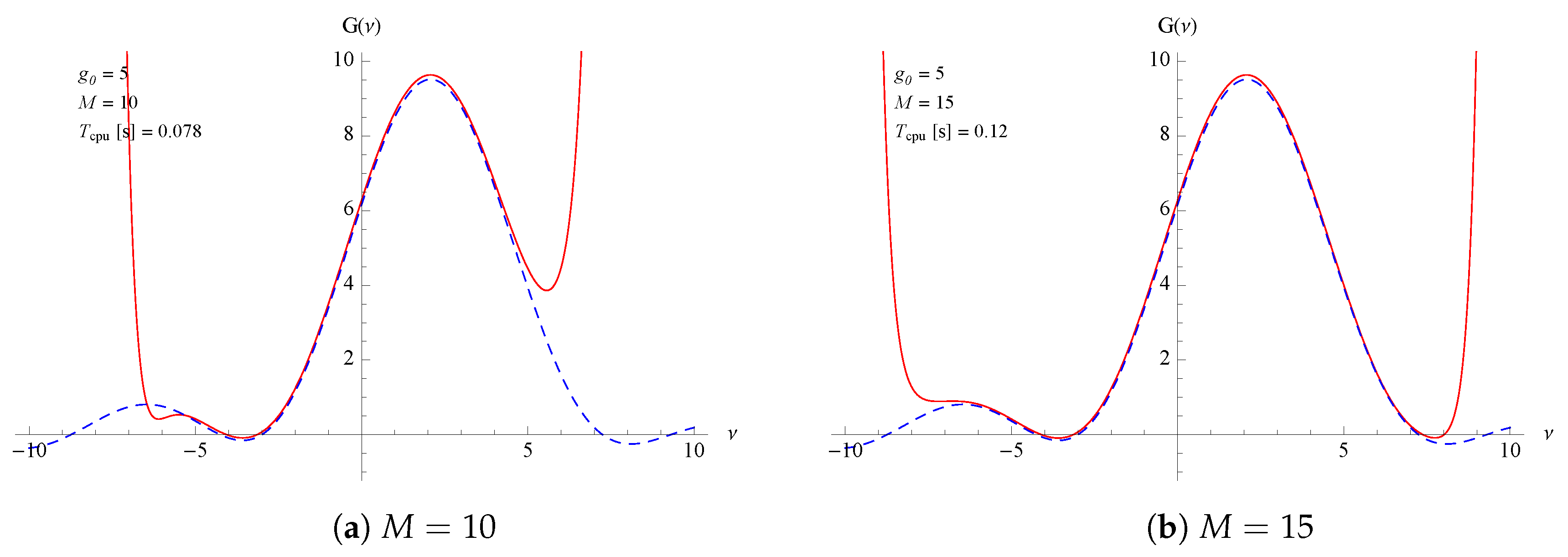
The comparison is reported in Figure 1 for a 2nd order gain function, where the present procedure (at different truncation levels) is confronted with those from a complete numerical integration and no differences are foreseeable. The truncation of the Hermite expansion obviously affects the speed and the approximation of the gain curve.

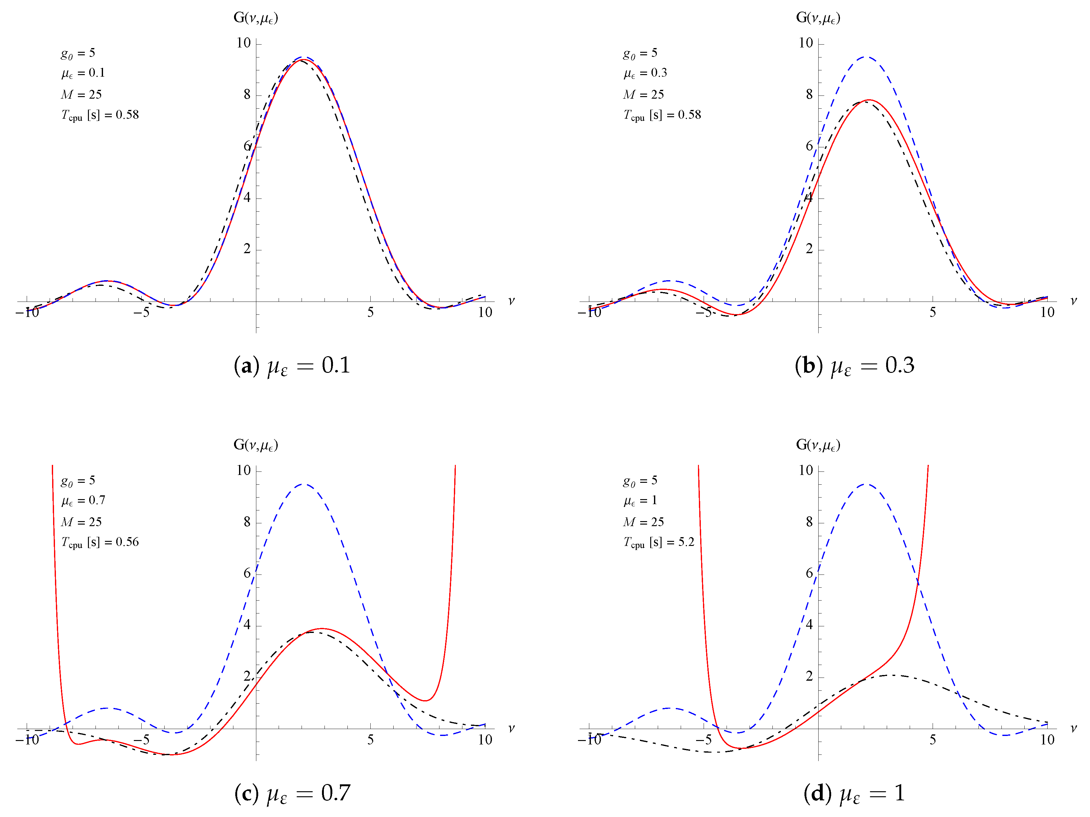
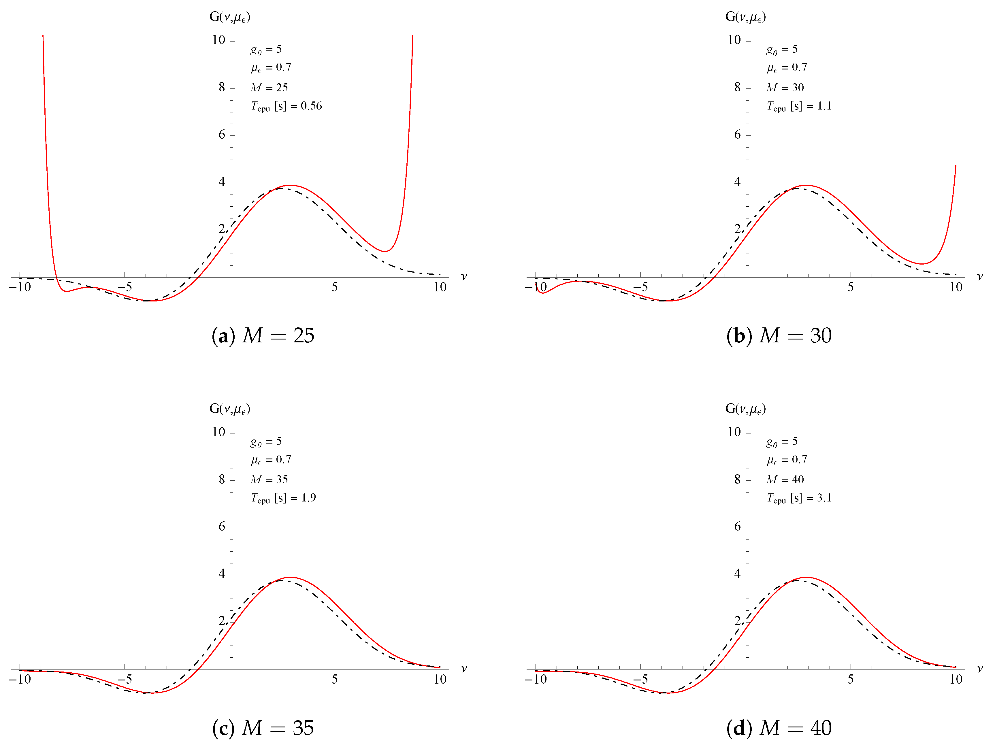
The method allows also taking into account the broadening effect as shown in Figure 2. It has to be noted that for higher broadening effects an higher truncation level is needed to achieve a good approximation, as shown in Figure 3. In this case, the comparison is made with the expression discussed in Appendix B.

The Hermite expansion approach let the integrals found in Equation (6) become polynomials and thus very easy to solve automatically. They are, of course, high in number but tractable also by a symbolic processor.

It is therefore possible to obtain, with the same degree of approximation, but with longer calculation times than the numeric case, also the full analytical expression for the curve.

The longer timings are then well payed back by the possibility to evaluate the curve on the fly with any combination of parameter values.

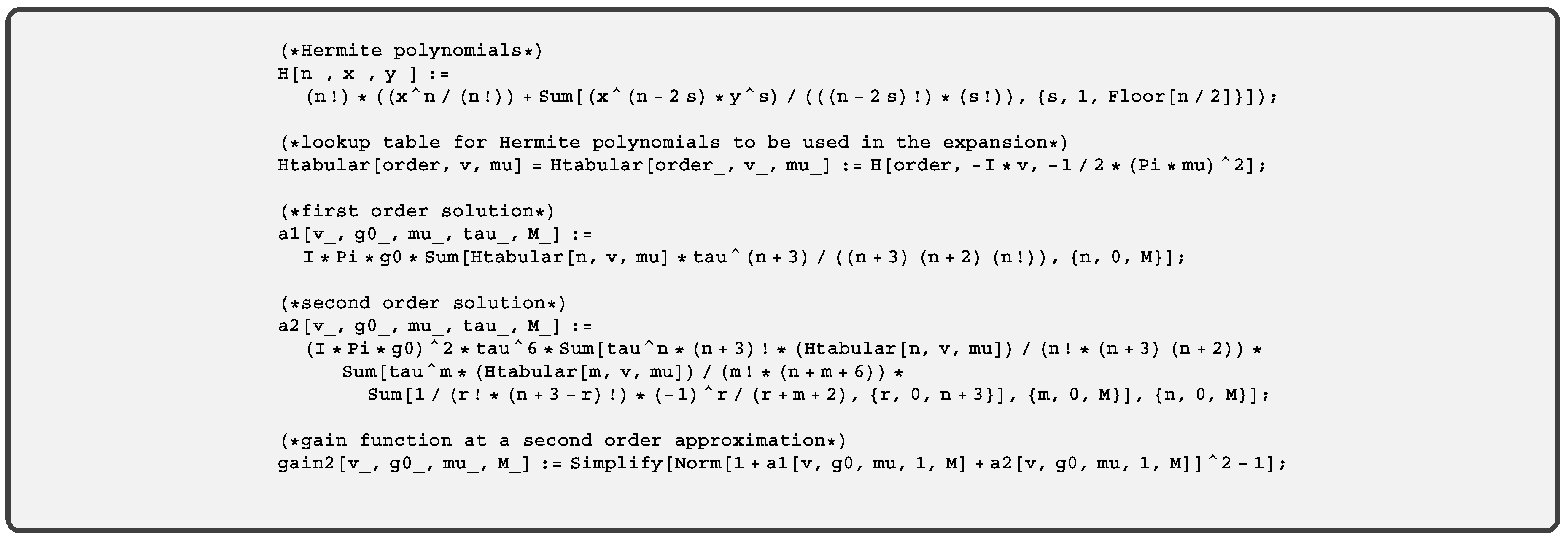
In Appendix A it can be found the symbolic expression of the curve for $M=10$ (which is inaccurate, but compact enough to be checked by visual inspection and corresponding to that plotted in Figure 1).

It is clear that in our procedure there are two levels of approximation, the first associated with the principal index expansion n, depending on the values of the small signal gain coefficient $g_0$ which fixes how fast the laser intensity grows in time, the second is associated with the nested index $m_n$ , depending on the values of the inhomogeneous parameter. It is worth noting that in actual FEL devices $n=4$ is largely sufficient and since ${\mu }_{\epsilon }$ is not larger than $0.3$ the index $m_n$ is not required to exceed 30.

4. Conclusions

The method we have foreseen is general enough to be applied to Volterra type equations with different kernels, provided that a corresponding expansion in terms of a suitable polynomial family is allowed.

To clarify the previous statement we consider the equation

$${\partial }_{\tau }a\left(\tau \right)=\lambda {\int }_0^{\tau }{\displaystyle \frac{{\tau }^{\prime }}{1+\alpha {\tau }^{\prime }+\beta {\tau }^{\prime 2}}}a(\tau -{\tau }^{\prime })d{\tau }^{\prime }$$

(17)

In this case the problem can be solved by the use of a two variable Legendre like polynomials

$$P_n(x,y)=\sum _{r=0}^{\lfloor \frac{n}{2}\rfloor }{\displaystyle \frac{(n-r)!x^{n-2r}{y}^r}{(n-2r)!r!}}$$

(18)

with generating function

$$\sum _{n=0}^{\infty }{t}^n{P}_n(x,y)={\displaystyle \frac{1}{1+xt+y{t}^2}}.$$

(19)

The solution of the problem (17) looks, therefore, like the expression derived for Equation (1) with the two variable Legendre polynomials replacing the Hermite polynomials, namely

$${\partial }_{\tau }{a}_n\left(\tau \right)=\lambda \sum _{m_n=0}^{\infty }{P}_{m_n}(-\alpha ,-\beta ){\int }_0^{\tau }{\tau }^{\prime (m_n+1)}{a}_{n-1}(\tau -{\tau }^{\prime })d{\tau }^{\prime }.$$

(20)

In a forthcoming paper, dedicated to the physical aspects of the FEL, we will show how this family of polynomials allows the inclusion in the FEL high gain equation of the gain detrimental effects due to electron beam transverse and angular distributions.