
New Analytical Technique for Solving a System of Nonlinear Fractional Partial Differential Equations


Abstract
:1. Introduction
2. Basic Definitions and Preliminaries
3. NAT for Solving a System of NFPDEs
3.1. Existence Theorem
3.2. Convergence and Error Analysis
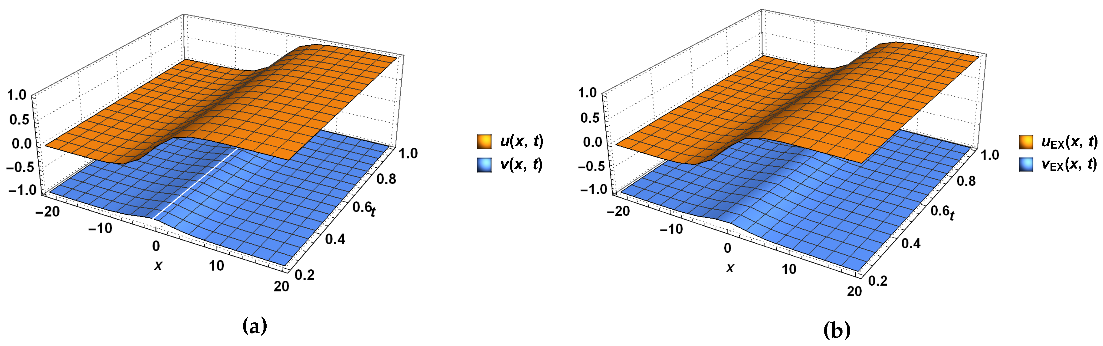
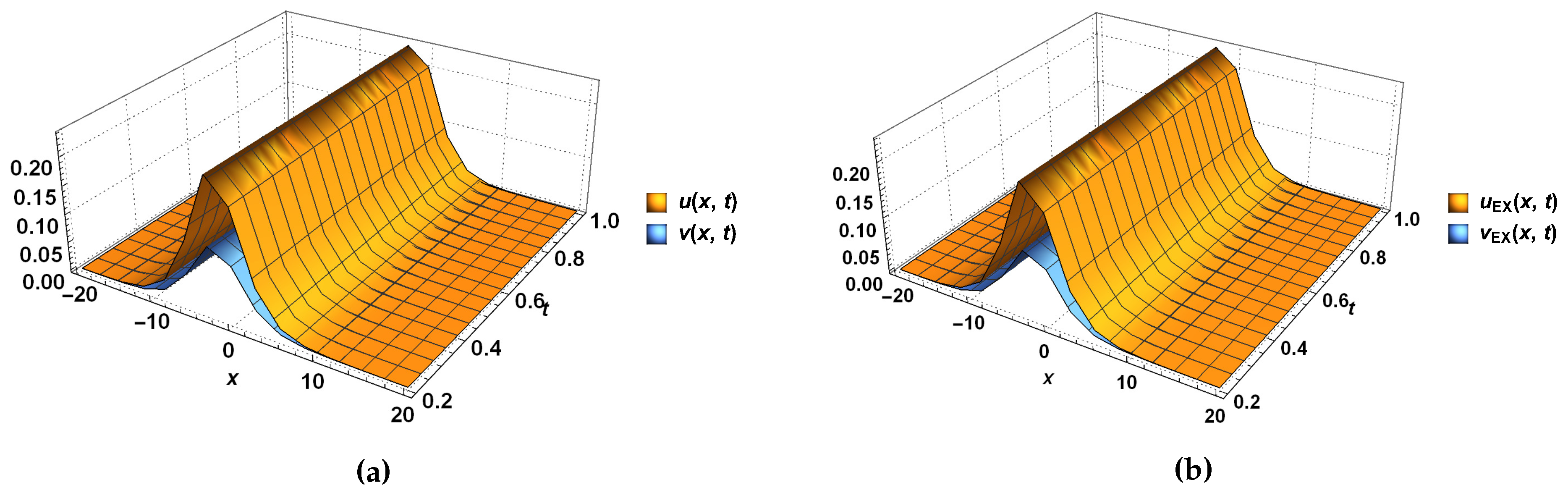
4. Applications to the Systems of Nonlinear Wave Equations
5. Discussion and Conclusions
Acknowledgments
Author Contributions
Conflicts of Interest
References
- Baleanu, D. Special issue on nonlinear fractional differential equations and their applications in honour of Ravi P. Agarwal on his 65th birthday. Nonlinear Dyn. 2013, 71, 603. [Google Scholar] [CrossRef]
- Chalishajar, D.; George, R.; Nandakumaran, A.; Acharya, F. Trajectory controllability of nonlinear integro-differential system. J. Franklin Inst. 2010, 347, 1065–1075. [Google Scholar] [CrossRef]
- De Souza, M. On a class of nonhomogeneous fractional quasilinear equations in with exponential growth. Nonlinear Differ. Equ. Appl. NoDEA. 2015, 22, 499–511. [Google Scholar] [CrossRef]
- Demir, A.; Erman, S.; Özgür, B.; Korkmaz, E. Analysis of fractional partial differential equations by Taylor series expansion. Bound. Value Probl. 2013, 2013, 68. [Google Scholar] [CrossRef]
- Huang, Q.; Zhdanov, R. Symmetries and exact solutions of the time fractional Harry-Dym equation with Riemann–Liouville derivative. Phys. A Stat. Mech. Appl. 2014, 409, 110–118. [Google Scholar] [CrossRef]
- Sun, H.; Chen, W.; Chen, Y. Variable-order fractional differential operators in anomalous diffusion modeling. Phys. A Stat. Mech. Appl. 2009, 388, 4586–4592. [Google Scholar] [CrossRef]
- Sun, H.; Chen, W.; Li, C.; Chen, Y. Fractional differential models for anomalous diffusion. Phys. A Stat. Mech. Appl. 2010, 389, 2719–2724. [Google Scholar] [CrossRef]
- Sun, H.G.; Chen, W.; Sheng, H.; Chen, Y.Q. On mean square displacement behaviors of anomalous diffusions with variable and random orders. Phys. Lett. A 2010, 374, 906–910. [Google Scholar] [CrossRef]
- Zayed, E.M.E.; Amer, Y.A.; Shohib, R.M.A. The fractional complex transformation for nonlinear fractional partial differential equations in the mathematical physics. J. Assoc. Arab Univ. Basic Appl. Sci. 2016, 19, 59–69. [Google Scholar] [CrossRef]
- Momani, S.; Odibat, Z. Homotopy perturbation method for nonlinear partial differential equations of fractional order. Phys. Lett. A 2007, 365, 345–350. [Google Scholar] [CrossRef]
- El-Sayed, A.; Elsaid, a.; El-Kalla, I.; Hammad, D. A homotopy perturbation technique for solving partial differential equations of fractional order in finite domains. Appl. Math. Comput. 2012, 218, 8329–8340. [Google Scholar] [CrossRef]
- Odibat, Z.; Momani, S. Numerical methods for nonlinear partial differential equations of fractional order. Appl. Math. Model. 2008, 32, 28–39. [Google Scholar] [CrossRef]
- Ma, W.X.; Lee, J.H. A transformed rational function method and exact solutions to the 3 + 1 dimensional Jimbo-Miwa equation. Chaos Solitons Fractals 2009, 42, 1356–1363. [Google Scholar] [CrossRef]
- Ma, W.X.; Zhu, Z. Solving the (3 + 1)-dimensional generalized KP and BKP equations by the multiple exp-function algorithm. Appl. Math. Comput. 2012, 218, 11871–11879. [Google Scholar] [CrossRef]
- Magin, R.; Ortigueira, M.D.; Podlubny, I.; Trujillo, J. On the fractional signals and systems. Signal Proc. 2011, 91, 350–371. [Google Scholar] [CrossRef]
- Mamchuev, M.O. Cauchy problem in nonlocal statement for a system of fractional partial differential equations. Differ. Equ. 2012, 48, 354–361. [Google Scholar] [CrossRef]
- Mamchuev, M.O. Mixed problem for a system of fractional partial differential equations. Differ. Equ. 2016, 52, 133–138. [Google Scholar] [CrossRef]
- Longuet-Higgins, M.; Stewart, R. Radiation stresses in water waves; a physical discussion, with applications. Deep Sea Res. Oceanogr. Abstr. 1964, 11, 529–562. [Google Scholar] [CrossRef]
- Slunyaev, A.; Didenkulova, I.; Pelinovsky, E. Rogue waters. Contemp. Phys. 2011, 52, 571–590. [Google Scholar] [CrossRef]
- Bai, C. New explicit and exact travelling wave solutions for a system of dispersive long wave equations. Rep. Math. Phys. 2004, 53, 291–299. [Google Scholar] [CrossRef]
- Benney, D.J.; Luke, J.C. On the Interactions of Permanent Waves of Finite Amplitude. J. Math. Phys. 1964, 43, 309–313. [Google Scholar] [CrossRef]
- Wang, M. Solitary wave solutions for variant Boussinesq equations. Phys. Lett. A 1995, 199, 169–172. [Google Scholar] [CrossRef]
- Lu, B. N-soliton solutions of a system of coupled KdV equations. Phys. Lett. A 1994, 189, 25–26. [Google Scholar] [CrossRef]
- Wang, M.; Zhou, Y.; Li, Z. Application of a homogeneous balance method to exact solutions of nonlinear equations in mathematical physics. Phys. Lett. A. 1996, 216, 67–75. [Google Scholar] [CrossRef]
- Lou, S.Y. Painlevé test for the integrable dispersive long wave equations in two space dimensions. Phys. Lett. A 1993, 176, 96–100. [Google Scholar] [CrossRef]
- Paquin, G.; Winternitz, P. Group theoretical analysis of dispersive long wave equations in two space dimensions. Phys. D Nonlinear Phenom. 1990, 46, 122–138. [Google Scholar] [CrossRef]
- Jafari, H.; Seifi, S. Solving a system of nonlinear fractional partial differential equations using homotopy analysis method. Commun. Nonlinear Sci. Numer. Simul. 2009, 14, 1962–1969. [Google Scholar] [CrossRef]
- Jafari, H.; Nazari, M.; Baleanu, D.; Khalique, C.M. A new approach for solving a system of fractional partial differential equations. Comput. Math. Appl. 2013, 66, 838–843. [Google Scholar] [CrossRef]
- Zhang, R.; Gong, J. Synchronization of the fractional-order chaotic system via adaptive observer. Syst. Sci. Control Eng. 2014, 2, 751–754. [Google Scholar] [CrossRef]
- Diethelm, K. The Analysis of Fractional Differential Equations: An Application-Oriented Exposition Using Differential Operators of Caputo Type; Springer: Berlin, Germany, 2010. [Google Scholar]
- Ghorbani, A. Toward a new analytical method for solving nonlinear fractional differential equations. Comput. Methods Appl. Mech. Eng. 2008, 197, 4173–4179. [Google Scholar] [CrossRef]
- Guo, B.; Pu, X.; Huang, F. Fractional Partial Differential Equations and Their Numerical Solutions; World Scientific Publishing Co Pte Ltd: Singapore, 2015. [Google Scholar]
- Kilbas, A.A.A.; Srivastava, H.M.; Trujillo, J.J. Theory and Applications of Fractional Differential Equations; Elsevier Science Limited: Amsterdam, Netherlands, 2006; Volume 204. [Google Scholar]
- Miller, K.S.; Ross, B. An Introduction to the Fractional Calculus and Fractional Differential Equations; Wiley-Interscience: New York, NY, USA, 1993. [Google Scholar]
- Podlubny, I. Fractional Differential Equations: An Introduction to Fractional Derivatives, Fractional Differential Equations, to Methods of Their Solution and Some of Their Applications; Academic Press: Salt Lake City, UT, USA, 1998; p. 198. [Google Scholar]

| x | t | , | Absolute Error | ||||||
|---|---|---|---|---|---|---|---|---|---|
| −10 | 0.20 | 0.0171378 | 0.0085689 | 0.0174511 | 0.0087256 | 0.0174511 | 0.0087256 | 9.11712 × | 4.55856 × |
| 0.40 | 0.0169274 | 0.0084637 | 0.0172419 | 0.0086210 | 0.0172419 | 0.0086210 | 1.45834 × | 7.29172 × | |
| 0.60 | 0.0167686 | 0.0083843 | 0.0170352 | 0.0085176 | 0.0170352 | 0.0085176 | 7.38075 × | 3.69037 × | |
| 0 | 0.20 | 0.1994480 | 0.0997242 | 0.1977450 | 0.0988724 | 0.1977450 | 0.0988724 | 5.11989 × | 2.55994 × |
| 0.40 | 0.2006050 | 0.1003020 | 0.1988720 | 0.0994360 | 0.1988720 | 0.0994360 | 8.07505 × | 4.03753 × | |
| 0.60 | 0.20148400 | 0.1007420 | 0.1999930 | 0.0999966 | 0.1999930 | 0.0999966 | 4.02841 × | 2.01421 × | |
| 20 | 0.20 | 0.0000172 | 8.62 × | 0.0000169 | 8.46 × | 0.0000169 | 8.46 × | 1.70233 × | 8.51164 × |
| 0.40 | 0.0000175 | 8.74 × | 0.0000171 | 8.56 × | 0.0000171 | 8.56 × | 2.73056 × | 1.36528 × | |
| 0.60 | 0.0000177 | 8.83 × | 0.0000173 | 8.67 × | 0.0000173 | 8.67 × | 1.38582 × | 6.92909 × | |
| x | t | Absolute Error | |||||||
|---|---|---|---|---|---|---|---|---|---|
| −10 | 0.20 | 0.0104859 | −0.9952150 | 0.0104567 | −0.9948260 | 0.0104567 | −0.9948260 | 2.38731 × | 9.68267 × |
| 0.40 | 0.0100181 | −0.9954506 | 0.0099518 | −0.9950740 | 0.0099518 | −0.9950740 | 3.78897 × | 1.54049 × | |
| 0.60 | 0.0095700 | −0.9956240 | 0.0094709 | −0.9953090 | 0.0094710 | −0.9953090 | 1.90276 × | 7.75425 × | |
| 0 | 0.20 | 0.6103320 | −0.8796460 | 0.6106390 | −0.8811210 | 0.6106390 | −0.8811210 | 2.69185 × | 1.81638 × |
| 0.40 | 0.5979280 | −0.8788030 | 0.5986870 | −0.8798700 | 0.5986880 | −0.8798700 | 4.24645 × | 2.98579 × | |
| 0.60 | 0.5853820 | −0.8782520 | 0.5866150 | −0.8787530 | 0.5866180 | −0.8787510 | 2.11781 × | 1.55116 × | |
| 20 | 0.20 | 0.9999710 | −0.9999840 | 0.9999710 | −0.9999860 | 0.9999710 | −0.9999860 | 7.23998 × | 3.61844 × |
| 0.40 | 0.9999700 | −0.9999830 | 0.9999700 | −0.9999850 | 0.9999000 | −0.9999850 | 1.17016 × | 5.84818 × | |
| 0.60 | 0.9999680 | −0.9999820 | 0.9999680 | −0.9999840 | 0.9999680 | −0.9999840 | 5.98445 × | 2.99087 × | |
© 2017 by the authors. Licensee MDPI, Basel, Switzerland. This article is an open access article distributed under the terms and conditions of the Creative Commons Attribution (CC BY) license (http://creativecommons.org/licenses/by/4.0/).
Share and Cite
Thabet, H.; Kendre, S.; Chalishajar, D. New Analytical Technique for Solving a System of Nonlinear Fractional Partial Differential Equations. Mathematics 2017, 5, 47. https://doi.org/10.3390/math5040047
Thabet H, Kendre S, Chalishajar D. New Analytical Technique for Solving a System of Nonlinear Fractional Partial Differential Equations. Mathematics. 2017; 5(4):47. https://doi.org/10.3390/math5040047
Chicago/Turabian StyleThabet, Hayman, Subhash Kendre, and Dimplekumar Chalishajar. 2017. "New Analytical Technique for Solving a System of Nonlinear Fractional Partial Differential Equations" Mathematics 5, no. 4: 47. https://doi.org/10.3390/math5040047
APA StyleThabet, H., Kendre, S., & Chalishajar, D. (2017). New Analytical Technique for Solving a System of Nonlinear Fractional Partial Differential Equations. Mathematics, 5(4), 47. https://doi.org/10.3390/math5040047