Abstract
Burg’s entropy plays an important role in this age of information euphoria, particularly in understanding the emergent behavior of a complex system such as statistical mechanics. For discrete or continuous variable, maximization of Burg’s Entropy subject to its only natural and mean constraint always provide us a positive density function though the Entropy is always negative. On the other hand, Burg’s modified entropy is a better measure than the standard Burg’s entropy measure since this is always positive and there is no computational problem for small probabilistic values. Moreover, the maximum value of Burg’s modified entropy increases with the number of possible outcomes. In this paper, a premium has been put on the fact that if Burg’s modified entropy is used instead of conventional Burg’s entropy in a maximum entropy probability density (MEPD) function, the result yields a better approximation of the probability distribution. An important lemma in basic algebra and a suitable example with tables and graphs in statistical mechanics have been given to illustrate the whole idea appropriately.
1. Introduction
The concept of entropy [1] figured strongly in the physical sciences during the 19th century, especially in thermodynamics and statistical mechanics [2], as a measure of equilibrium and evolution of thermodynamic systems. Two main views were developed which were the macroscopic view formulated originally by Clausius and Carnot and the microscopic approach associated with Boltzmann and Maxwell. Since then, both the approaches have made introspection in natural thermodynamic and microscopically probabilistic systems possible. Entropy is defined as the measure of a system’s thermal energy per unit temperature that is unavailable for doing useful work. Because work is obtained from ordered molecular motion, the amount of entropy is also a measure of molecular disorder or randomness of a system. The concept of entropy provides deep insight into the direction of spontaneous change for many day-to-day phenomena. Now, how entropy was developed by Rudolf Clausius [3] is discussed below.
1.1. Clausius’s Entropy
To provide a quantitative measure for the direction of spontaneous change, Clausius introduced the concept of entropy as a precise way of expressing the second law of thermodynamics. The Clausius form of the second law states that spontaneous change for an irreversible process [4] in an isolated system (that is, one that does not exchange heat or work with its surroundings) always proceeds in the direction of increasing entropy. By the Clausius definition, if an amount of heat flows into a large heat reservoir at temperature above absolute zero, then . This equation effectively gives an alternate definition of temperature that agrees with the usual definition. Assume that there are two heat reservoirs and at temperatures and . (such as the stove and the block of ice). If an amount of heat flows from to , then the net entropy change for the two reservoirs is which is positive, provided that . Thus, the observation that heat never flows spontaneously from cold to hot is equivalent to requiring the net entropy change to be positive for a spontaneous flow of heat. When the system is in thermodynamic equilibrium, then , i.e., if , then the reservoirs are in equilibrium, no heat flows, and . If the gas absorbs an incremental amount of heat from a heat reservoir at temperature and expands reversibly against the maximum possible restraining pressure , then it does the maximum work and . The internal energy of the gas might also change by an amount as it expands. Then, by conservation of energy, . Because the net entropy change for the system plus reservoir is zero when maximum work is done and the entropy of the reservoir decreases by an amount , this must be counterbalanced by an entropy increase of for the working gas so that . For any real process, less than the maximum work would be done (because of friction, for example), and so the actual amount of heat absorbed from the heat reservoir would be less than the maximum amount . For example, the gas could be allowed to expand freely into a vacuum and do no work at all. Therefore, it can be stated that with, in the case of maximum work corresponding to a reversible process. This equation defines as a thermodynamic state variable, meaning that its value is completely determined by the current state of the system and not by how the system reached that state. Entropy is a comprehensive property in that its magnitude depends on the amount of material in the system.
In one statistical interpretation of entropy, it is found that for a very large system in thermodynamic equilibrium, entropy is proportional to the natural logarithm of a quantity corresponding to and can be realized; that is, , in which is related to molecular energy. On the other hand, entropy generation analysis [5,6,7,8,9,10,11] is used to optimize the thermal engineering devices for higher energy efficiency; it has attracted wide attention to its applications and rates in recent years. In order to access the best thermal design of systems, by minimizing the irreversibility, the second law of thermodynamics could be employed. Entropy generation is a criterion for the destruction of a systematized work.The development of the theory followed two conceptually different lines of thought. Nevertheless, they are symbiotically related, in particular through the work of Boltzmann.
1.2. Boltzmann’s Entropy
In addition to thermodynamic (or heat-change) entropy, physicists also study entropy statistically [12,13]. The statistical or probabilistic study of entropy is presented in Boltzmann’s law. Boltzmann’s equation is somewhat different from the original Clausius (thermodynamic) formulation of entropy. Firstly, the Boltzmann formulation is structured in terms of probabilities, while the thermodynamic formulation does not consist in the calculation of probabilities. The thermodynamic formulation can be characterized as a mathematical formulation, while the Boltzmann formulation is statistical. Secondly, the Boltzmann equation yields a value of entropy while the thermodynamic formulation yields only a value for the change in entropy . Thirdly, there is a shift in content, as the Boltzmann equation was developed for research on gas molecules rather than thermodynamics. Fourthly, by incorporating probabilities, the Boltzmann equation focuses on microstates, and thus explicitly introduces the question of the relationship between macrostates and microstates. Boltzmann investigated such microstates and defined entropy in a new way such that the macroscopic maximum entropy state corresponded to a thermodynamic configuration which could be formulated by the maximum number of different microstates. He noticed that the entropy of a system can be considered as a measure of the disorder in the system and that in a system having many degrees of freedom, the number measuring the degree of disorder also measured the uncertainty in a probabilistic sense about the particular microstates.
The value was originally intended to be proportional to the Wahrscheinlichkeit (means probability) of a macrostate for some probability distribution of a possible microstate, in which the thermodynamic state of a system can be realized by assigning different and of different molecules. The Boltzmann formula is the most general formula for thermodynamic entropy; however, his hypothesis was for an ideal gas of identical particles, of which are the th microscopic condition of position and momentum of a given distribution . Here, , ,…etc. For this state, the probability of each microstate system is equal, so it was equivalent to calculating the number of microstates associated with a macrostate. Then the statistical disorder is given by [14] . Therefore, the entropy given by Boltzmann is: Where
Let us now take an approximate value of for a large . Using Stirling’s approximation , we have:
where is the probability of the occurrence of th microstates. Boltzmann was the first to emphasize the probabilistic meaning of entropy and the probabilistic nature of thermodynamics.
1.3. Information Theory andShannon’s Entropy
Unlike the first two entropy approaches (thermodynamic entropy by Clausius and Boltzmann’s entropy), the third major form of entropy did not fall within the field of physics, but was developed instead in a new field known as information theory [15,16,17] (also known as communication theory). A fundamental step in using entropy in new contexts unrelated to thermodynamics was provided by Shannon [18], who came to conclude that entropy could be used to measure types of disorder other than that of thermodynamic microstates. Shannon was interested in information theory [19,20], particularly in the ways in which information can be conveyed via a message. This led him to examine probability distributions in a very general sense and he worked to find a way of measuring the level of uncertainty in different distributions.
For example, suppose the probability distribution for the outcome of a coin toss experiment is P(H) = 0.999 and P(T) = 0.001. One is likely to notice that there is much more “certainty” than “uncertainty” about the outcome of this experiment and, consequently, the probability distribution. If, on the other hand, the probability distribution governing that same experiment were P(H) = 0.5 and P(T) = 0.5, then there is much less “certainty” and much more “uncertainty” when compared to the previous distribution. However, how can these uncertainties can be quantified? Is there some algebraic function which measures the amount of uncertainty in any probabilistic distribution in terms of the individual probabilities? From these types of simple examples and others, Shannon was able to devise a set of criteria which any measure of uncertainty may satisfy. He then tried to find an algebraic form which would satisfy his criteria and discovered that there was only one formula which fit. Let the probabilities of possible outcomes of an experiment be , giving rise to the probability distribution . There is an uncertainty as to the outcome when the experiment is performed. Shannon suggested the measure , which is identical to the previous entropy relation if the constant of probability is taken as the Boltzmann constant . Thus, Shannon showed that entropy, which measures the amount of disorder in a thermodynamic system, also measures the amount of uncertainty in any probability distribution. Let us now give the formal definition of Shannon’s entropy as follows: Consider a random experiment whose possible outcomes have probabilities that are known. Can we guess in advance which outcome we shall obtain? Can we measure the amount of uncertainty? We shall denote such an uncertainty measure by . The most common as well as the most useful measure of uncertainty is Shannon's informational entropy (which should satisfy some basic requirements), which is defined as follows:
Definition I:
Let be the probability of the occurrence of the events associated with a random experiment. The Shannon’s entropy probability distribution of the random experiment system is defined by where, . The above definition is generalized straightforwardly as the definition of entropy of a random variable.
Definition II: Let X R be a discrete random variable which takes the value with the probability ; then the entropy of is defined by the expression Examination of H or reveals why Shannon’s measure is the most satisfactory measure of entropy because of the following:
- (i)
- is a continuous function of
- (ii)
- is a symmetric function of its arguments.
- (iii)
- , i.e., it should not change if there is an impossible outcome to the probability.
- (iv)
- Its minimum is 0 when there is no uncertainty about the outcome. Thus, it should vanish when one of the outcomes is certain to happen so that
- (v)
- It is the maximum when there is maximum uncertainty, which arises when the outcomes are equally likely so that is the maximum when .
- (vi)
- The maximum value of increases with .
- (vii)
- For two independent probability distributions and , the uncertainty of the joint scheme should be the sum of their uncertainties:
Shannon’s entropy has various applications in the field of portfolio analysis, the measurement of economic analysis, transportation, and urban and regional planning as well as in the fields of statistics, thermodynamics, queuing theory, parametric estimation, etc. It has been used in the field non-commensurable and conflicting criteria [21] and in the nonlinear complexity of random sequences [22] as well.
2. Discussion
2.1. Jaynes’ Maximum Entropy (MaxEnt) Principle
Let the random variable of an experiment be , and assume the probability mass associated with the value is , i.e., . The set is called the source ensemble as described by Karmeshu [23]. In general, we may find expected values of the functions to get and with natural constraint given a number of constraints. Thus, we have relations between . There may be infinite probability distributions satisfying the above equation. If we know only , then we get a family of max entropy distributions. If, in addition, we know the values of we get a specific member of this family and we call it the max entropy probability distribution. According to a great article by Jaynes [24,25,26], we choose the probability distribution out of all these which maximizes the measure of entropy as shown by Shannon’s equation, .
Any distribution of the form may be regarded as the maximum entropy distribution where are determined as functions of ; then the maximum entropy is given by .
Kapur [27,28] showed that there is always a concave function of We also note that all the probabilities given by are always positive. We naturally want to know whether there is another measure of entropy other than Shannon’s entropy which, when maximized, subject to, , gives positive probabilities and for which is possibly a concave function [29] of parameters. Kapur [30] studied that Burg’s [31] measure of entropy, which has been very successfully used in spectral analysis, does always give positive probabilities. The maximum entropy principal of Jaynes has been used frequently to derive the distribution of statistical mechanics by maximizing the entropy of the system subject to some given constraints. The Maxwell-Boltzman distribution is obtained when there is only one constraint on a system which prescribes the expected energy per particle of the system by Bose-Einstein (B.E.) distribution, Fermi-Dirac (F.D.) distribution and intermediate statistics (I.S.) distributions; these are obtained by maximizing the entropy subject to two constraints by Kapur and Kesavan, and Kullback [32,33] and also by the present authors [34].
2.2. Formulation of MEPD in Statistical Mechanics Using Shannon’s Measure of Entropy
Let be the probabilities of a particle having energy levels ….,, respectively, and let the expected value of energy be prescribed as ; then, to get MEPD, we maximize the Shannon’s measure of entropy:
Subject to
Let the Lagrangian be
Differentiating with respect to ’s, we get:
where, are to be determined by using Equation (2) so that
Where
Equation (4) is the well-known Maxwell-Boltzmann distribution from statistical mechanics which is used in many areas [35,36,37].
2.3. Burg’s Entropy Measure and MEPD
When was replaced by Burg’s measure of entropy , it gave interesting results as shown by Kapur. Burg’s measure of entropy is always negative, but this does not matter in entropy maximization, where it has been found that a probability distribution with maximum entropy satisfies the same constraint and it does not matter if all the entropies are negative. So, in Equation (1) when we use
we get
where are obtained by solving the equations
Multiplying first and second Equation (8) by respectively then adding
We get
so that from Equation (8),
Then, is an obvious solution but that will give us and this will satisfy the second equation of (8)
if . Now, Equation (10) is the th degree polynomial in , and one of its roots is zero. Its non-zero solutions will be obtained by solving an equation of th degree in . Lemma has been proved by Kapur as the following:
Lemma:
All the roots of are real; in other words, none of the roots can be complex.
Proof:
Let be a pair of complex conjugate roots of Equation (10). Then,
and ; subtracting the second from the first, we get
, which gives , or . The second possibility can easily be ruled out. To find the actual location of the n real roots, let us assume
and this function is discontinuous at the following points:
, where and is a “+” fraction. More precisely, when points from one side and when points from other side. Again,
2.4. d Burg’s Modifie Entropy (MBE) Measure and MEPD
2.4.1. Monotonic Character of MBE
We propose use of Burg’s modified entropy instead of Burg’s entropy. Maximizing the Burg’s modified measure of entropy:
Therefore, is the monotonic increasing function of . For the probability distribution
it is showed (see: Table 1.) that .

Table 1.
The values & maximum values of Burg’s Modified Entropy.
The measure of entropy is the Burg’s modified entropy. This is a better measure than the standard Burg’s measure since it is always positive and there is no computational problem when is very small. In the above case, the maximum value increases with the number of possible outcomes .
2.4.2. MBE and Its Relation with Burg’s Entropy
So, when , maximizing and will give the same result in both cases;again, if is maximized under the constraints
we get . Letting, we have
The ’s are determined by using Constraints (14) and (15) and this gives the MEPD when Burg’s entropy is maximized as subject to Equation (14).
Therefore, when , the MEPD of BME Burg’s MEPD; in fact:
2.4.3. MBE and Its Concavity of under Prescribed Mean
subjectto .
We obtain this using Lagranges multiplier mechanics:
From the above equation:
, i.e., and
So
Therefore,
and
where is determined as a function of and that is
Therefore,
So that
will be a concave function of if , that is, if either when the denominator , respectively.
In the above case, when we get and the derivative of as follows:
So that
Additionally, we have
So that
Therefore,
So,
Therefore, from Equations (27) and (30),
will be a concave function of if either
Or
Additionally, when , all the probabilities are equal, and from Equation (24) we have:
We have,
Now, if we proceed algebraically as done Section 2.3, we get:
. The obvious solution of the above problem is which will give , i.e., uniform distribution, and thus we get, .
3. An Illustrative Example in Statistical Mechanics
3.1. Example
Let be the probabilities of a particle having energy levels ….,; respectively, and let the expected value of energy be prescribed as ; then, we get the maximum entropy probability distribution (MEPD) with MBE as follows:
Solution:
Maximizing the measure of entropy subject to the given constraints, we have .
When , i.e., , we get the probability distribution in the form of a table and also get the values of as described by Kapur and Kesavan.
There may be two cases,
Case (i) when .
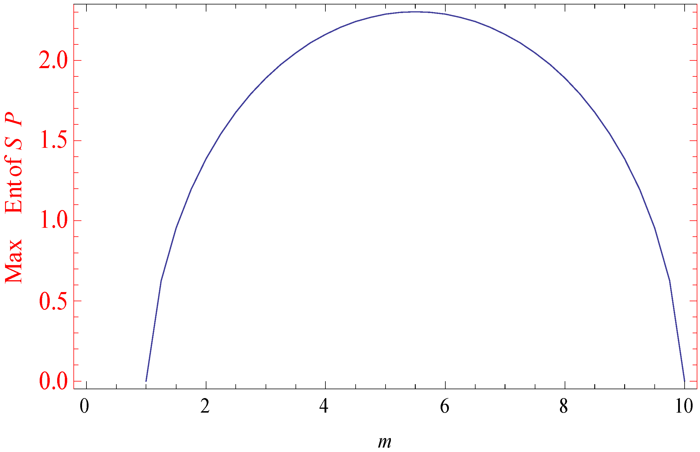
In this case, when lies between 1 and 5.5, implies and then is increasing.
Case (ii) when .
In this case, when lies between 5.5 and 10, implies and then is decreasing.
When , , .
it can be shown that will be concave if we prescribe instead of , where is a monotonic increasing function of ; then we will apply the necessary changes. Again, since the concavity of has already been proven, this will enable us to handle the inequality constraint of the type .
3.2. Simulated Results
Following Table (Table 2) Found Using LINGO Software 2011 where Different Max-Entropy Values Are Given for Different m Values:
Table 2.
Comparative Maximum Entropy Values.
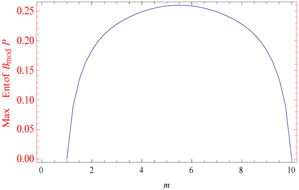
Figure 1.
Maximum Burg’s modified entropy.
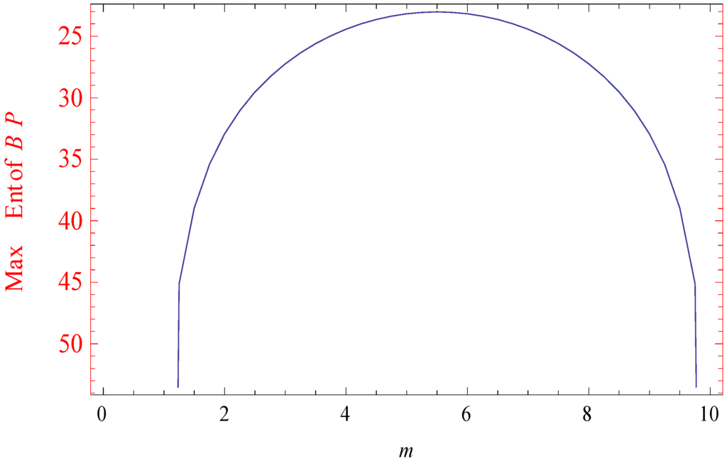
Figure 2.
Maximum Burg’s entropy.
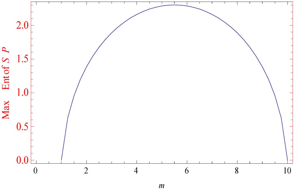
Figure 3.
Maximum Shannon’s entropy.
Table 3.
and graph.

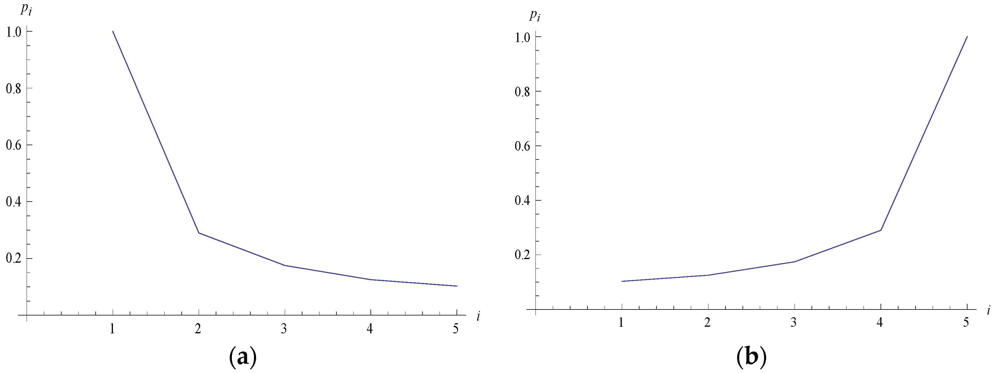
Figure 4.
Rectangular hyperbolic types of graphs. (a) when ; (b) when .
4. Conclusions
In the present paper we have presented different MEPDs and respective entropy measures with their properties. It has been found that MBE is a better measure than Burg’s entropy when the maximized subject to the mean is prescribed, and it also has been shown that unlike Burg’s entropy, the maximum value of MBE increases with . The main problem here will consist of solving simultaneous transcendental equations for the Lagranges multipliers. An application in statistical mechanics with simulated data has been studied with the help of Lingo11 software and corresponding graphs are provided. Now, one question arises: Will this result continue to hold for other moment constraints also? When we take generalized moment expectation of instead of expectation of , then must be a monotonic increasing function of , and if becomes negative for some values of the moments, then we have to set those probabilities to zero and reformulate the problem for the remaining probabilities over the remaining range and solve it.
Acknowledgments
Authors would like to express their sincere gratitude and appreciation to the reviewers for their valuable comments and good suggestions to make this paper enriched and impactful, and a special thank you to the Assistant Editor.
Author Contributions
A. Ray and S. K. Majumder conceived and designed the experiments; A. Ray performed the experiments, analyzed the data and both A. Ray and S. K. Majumder contributed in analysis tools; A. Ray wrote the paper.
Conflicts of Interest
The authors declare no conflict of interest.
Nomenclature
- = Entropy
- , probability of th event
- = Information entropy
- = Shannon’s entropy
- = Burg’s entropy
- = Burg’s modified entropy
- = Number of energy levels/number of possible outcome
- = Boltzmann constant
- = Absolute temperature
- = Identical particle of ideal gas
- = Increase of entropy
- = Change in entropy
- = Greatest integer value of
- Where is the mean value:
- = Expectation
- = Change in volume
- = Union of two sets
- , ranges from 1 to 10 with step length of 0.25
- = Maximum entropy
- = Maximum value under the given probability distribution
- MBE=Modified Burg’s Entropy
Greek Symbols
- = The maximum number of microscopic ways in the macroscopic state
- = Position of the molecule
- = Momentum of the molecule
- =Lagrangian constant
- =Different energy levels
- =Mean energy
Subscripts
- B=Boltzmann
- max =Maximum
- mod =modified
Superscript
- =New constant different from
References
- Andreas, G.; Keller, G.; Warnecke, G. Entropy; Princeton University Press: Princeton, NJ, USA, 2003. [Google Scholar]
- Phil, A. Thermodynamics and Statistical Mechanics: Equilibrium by Entropy Maximisation; Academic Press: Cambridge, MA, USA, 2002. [Google Scholar]
- Rudolf, C. Ueber verschiedene für die Anwendung bequeme Formen der Hauptgleichungen der mechanischen Wärmetheorie. Annalen der Physik 1865. (In German) [Google Scholar] [CrossRef]
- Wu, J. Three Factors Causing the Thermal Efficiency of a Heat Engine to Be Less than Unity and Their Relevance to Daily Life. Eur. J. Phys. 2015, 36, 015008. [Google Scholar] [CrossRef]
- Rashidi, M.M.; Shamekhi, L. Entropy Generation Analysis of the Revised Cheng-Minkowycz Problem for Natural Convective Boundary Layer Flow of Nanofluid in a Porous Medium. J. Thermal Sci. 2015, 19. [Google Scholar] [CrossRef]
- Rashidi, M.M.; Mohammadi, F. Entropy Generation Analysis for Stagnation Point Flow in a Porous Medium over a Permeable Stretching Surface. J. Appl. Fluid Mech. 2014, 8, 753–763. [Google Scholar]
- Rashidi, M.M.; Mahmud, S. Analysis of Entropy Generation in an MHD Flow over a Rotating Porous Disk with Variable Physical Properties. Int. J. Energy 2014. [Google Scholar] [CrossRef]
- Abolbashari, M.H.; Freidoonimehr, N. Analytical Modeling of Entropy Generation for Casson Nano-Fluid Flow Induced by a Stretching Surface. Adv. Powder Technol. 2015, 231. [Google Scholar] [CrossRef]
- Baag, S.S.R.; Dash, M.G.C.; Acharya, M.R. Entropy Generation Analysis for Viscoelastic MHD Flow over a Stretching Sheet Embedded in a Porous Medium. Ain Shams Eng. J. 2016, 23. [Google Scholar] [CrossRef]
- Shi, Z.; Tao, D. Entropy Generation and Optimization of Laminar Convective Heat Transfer and Fluid Flow in a Microchannel with Staggered Arrays of Pin Fin Structure with Tip Clearance. Energy Convers. Manag. 2015, 94, 493–504. [Google Scholar] [CrossRef]
- Hossein, A.M.; Ahmadi, M.A.; Mellit, A.; Pourfayaz, F.; Feidt, M. Thermodynamic Analysis and Multi Objective Optimization of Performance of Solar Dish Stirling Engine by the Centrality of Entransy and Entropy Generation. Int. J. Electr. Power Energy Syst. 2016, 78, 88–95. [Google Scholar] [CrossRef]
- Giovanni, G. Statistical Mechanics: A Short Treatise; Springer Science & Business Media: New York, NY, USA, 2013. [Google Scholar]
- Reif, F. Fundamentals of Statistical and Thermal Physics; Waveland Press: Long Grove, IL, USA, 2009. [Google Scholar]
- Rudolf, C.; Shimony, A. Two Essays on Entropy; University of California Press: Berkeley, CA, USA, 1977. [Google Scholar]
- Shu-Cherng, F.; Rajasekera, J.R.; Tsao, H.S.J. Entropy Optimization and Mathematical Programming; Springer Science & Business Media: New York, NY, USA, 2012. [Google Scholar]
- Robert, M.G. Entropy and Information Theory; Springer Science & Business Media: New York, NY, USA, 2013. [Google Scholar]
- Silviu, G. Information Theory with New Applications; MacGraw-Hill Books Company: New York, NY, USA, 1977. [Google Scholar]
- Shannon, C.E. A Mathematical Theory of Communication. SigmobileMob. Comput. Commun. Rev. 2001, 5, 3–55. [Google Scholar] [CrossRef]
- Thomas, M.C.; Thomas, J.A. Elements of Information Theory; John Wiley & Sons: Hoboken, NJ, USA, 2012. [Google Scholar]
- Christodoulos, A.F.; Pardalos, P.M. Encyclopedia of Optimization; Springer Science & Business Media: New York, NY, USA, 2008. [Google Scholar]
- Arash, M.; Azarnivand, A. Application of Integrated Shannon’s Entropy and VIKOR Techniques in Prioritization of Flood Risk in the Shemshak Watershed, Iran. Water Resour. Manag. 2015, 30, 409–425. [Google Scholar] [CrossRef]
- Liu, L.; Miao, S.; Liu, B. On Nonlinear Complexity and Shannon’s Entropy of Finite Length Random Sequences. Entropy 2015, 17, 1936–1945. [Google Scholar] [CrossRef]
- Karmeshu. Entropy Measures, Maximum Entropy Principle and Emerging Applications; Springer: Berlin, Germany; Heidelberg, Germany, 2012. [Google Scholar]
- Jaynes, E.T. Information Theory and Statistical Mechanics. II. Phys. Rev. 1957, 108, 171–190. [Google Scholar] [CrossRef]
- Jaynes, E.T. On the Rationale of Maximum-Entropy Methods. Proc. IEEE 1982, 70, 939–952. [Google Scholar] [CrossRef]
- Jaynes, E.T. Prior Probabilities. IEEE Trans. Syst. Sci. Cybernet. 1968, 4, 227–241. [Google Scholar] [CrossRef]
- Kapur, J.N. Maximum-Entropy Models in Science and Engineering; John Wiley & Sons: New York, NY, USA, 1989. [Google Scholar]
- Kapur, J.N. Maximum-Entropy Probability Distribution for a Continuous Random Variate over a Finite Interval. J. Math. Phys. Sci. 1982, 16, 693–714. [Google Scholar]
- Ray, A.; Majumder, S.K. Concavity of maximum entropy through modified Burg’s entropy subject to its prescribed mean. Int. J. Math. Oper. Res. 2016, 8. to appear. [Google Scholar]
- Kapur, J.N. Measures of Information and Their Applications; Wiley: New York, NY, USA, 1994. [Google Scholar]
- Burg, J. The Relationship between Maximum Entropy Spectra and Maximum Likelihood Spectra. Geophysics 1972, 37, 375–376. [Google Scholar] [CrossRef]
- Narain, K.J.; Kesavan, H.K. Entropy Optimization Principles with Applications; Academic Press: Cambridge, MA, USA, 1992. [Google Scholar]
- Solomon, K. Information Theory and Statistics; Courier Corporation: North Chelmsford, MA, USA, 2012. [Google Scholar]
- Amritansu, R.; Majumder, S.K. Derivation of some new distributions in statistical mechanics using maximum entropy approach. Yugoslav J. Oper. Res. 2013, 24, 145–155. [Google Scholar]
- Ulrych, T.J.; Bishop, T.N. Maximum Entropy Spectral Analysis and Autoregressive Decomposition. Rev. Geophys. 1975, 13, 183–200. [Google Scholar] [CrossRef]
- Michele, P.; Ferrante, A. On the Geometry of Maximum Entropy Problems. 2011. arXiv:1112.5529. [Google Scholar]
- Ke, J.-C.; Lin, C.-H. Maximum Entropy Approach to Machine Repair Problem. Int. J. Serv. Oper. Inform. 2010, 5, 197–208. [Google Scholar] [CrossRef]

© 2016 by the authors; licensee MDPI, Basel, Switzerland. This article is an open access article distributed under the terms and conditions of the Creative Commons by Attribution (CC-BY) license (http://creativecommons.org/licenses/by/4.0/).