1. Introduction and Statement of Results
The celebrated twin prime conjecture predicts that there are infinitely many pairs of consecutive primes. While a proof of the conjecture seems to be out of reach by current methods, there has been a spate of recent advances concerning the weaker conjecture:
In 2005, Goldston, Pintz and Yıldırım [
1] proved that there exists infinitely many consecutive primes, which are much closer than average, that is,
Based on their methods, Zhang [
2] showed that:
Maynard [
3] improved the upper bound to 600 using a modified sieve method. The constant was subsequently improved to 252 by an ongoing polymath project [
4].
In a similar vein, people have investigated related problems about “almost primes” or numbers with few prime factors. Chen [
5] proved that there are infinitely many primes,
p, such that
has at most two distinct prime factors. In [
6], Goldston, Graham, Pintz and Yıldırım (GGPY) considered the
numbers, which are numbers with exactly two distinct prime factors, and showed that there are infinitely many pairs of
numbers that are at most six apart.
Thorne [
7] observed that the methods in [
6] are highly adaptable, and generalized the result to
numbers, which are numbers with exactly
r distinct prime factors. In [
7], he showed that given an infinite set of primes,
, satisfying certain conditions, and positive integers
ν and
r with
, there exists an effectively computable constant
, such that:
where
is the
n-th
number, whose prime factors are all in
.
Using this theorem, Thorne proved several corollaries. With a result by Soundararajan [
8], he showed that there are infinitely many pairs of
numbers,
m and
n, such that the class groups,
and
, each contain elements of order four, with
. As a second application, he considered the quadratic twists of elliptic curves over
without a
-rational torsion point of order two. Let
be such an elliptic curve,
denote its Hasse–Weil
L-function,
denote the rank of the group of rational points on
E over
and
denote the
D-quadratic twist of
E for a fundamental discriminant,
D. Using the work of Ono [
9], he showed that for “good” elliptic curve
(defined as in [
10]), there are infinitely many pairs of square-free numbers,
m and
n, such that
,
and
hold simultaneously for some absolute constant,
. For
, Thorne obtained a bound of
6,152,146.
In this paper, we revisit Thorne’s examples and obtain stronger bounds by relaxing the condition to instead consider bounded gaps between square-free numbers with prime factors all in . In this case, we can prove an analogous general theorem with a better bound on the gaps.
Theorem 1. Suppose is a set of primes with positive Frobenius density. Let ν be a positive integer; and let denote the n-th square-free number, whose prime factors are all in . Then: Remark 1. Theorem 1 also holds for arbitrary sets of primes of positive density satisfying a Siegel–Walfisz-type condition (defined in
Section 2).
We observe that if we remove the restriction on the number of prime divisors in each of Thorne’s examples, we can obtain better bounds. Replacing by a square-free number in his first example, we obtain the following twin prime-type result.
Corollary 1. There are infinitely many square-free numbers, n, such that the class groups, and , each contain elements of order four.
In the second example, the bound, , can be improved analogously. We give an explicit bound in the case when .
Corollary 2. Let . Then, there are infinitely many pairs of square-free numbers, m and n, for which the following hold simultaneously:
- (i)
,
- (ii)
,
- (iii)
.
Remark 2. There are more general applications of Theorem 1. Thorne [
7] described an application to the nonvanishing of Fourier coefficients of weight one newforms, where Theorem 1 can also be applied. If
is a newform of integer weight, then the set of integers,
n, such that
is nonzero modulo
ℓ has zero density for all prime
ℓ by the theory of Deligne and Serre [
11]. Nonetheless, our result shows that there are bounded gaps between such
n for almost all
ℓ, yielding better bounds than [
7].
Our result also applies to the quadratic twists of elliptic curves over
that have a given 2-Selmer
-rank. If
K is a number field,
E is an elliptic curve over
K and
r is a suitable nonnegative integer, Mazur and Rubin [
12] conjecture that for a positive proportion of quadratic extensions,
, the quadratic twist,
, of
E by
has the 2-Selmer rank
r. Using ([
12] (Proposition 4.2)), our result shows that for
, an elliptic curve,
, with no two-torsion points, and a given integer,
, either no quadratic twists have 2-Selmer rank
r or there are bounded gaps between the square-free numbers,
d, such that
has 2-Selmer rank
r.
2. Main Result
We borrow our notation from [
6], using
k to denote an integer greater than one,
to denote an admissible
k-tuple of linear forms (defined in
Section 2.2) with
for some
, and
to denote a set of primes with positive density
α. The constants implied by “
O” and “≪” may depend on
k,
and
. Let
denote the number of ways of writing
n as a product of
k factors and
denote the number of distinct prime factors of
n.
and
are the usual Euler and Möbius functions.
N and
R will denote real numbers regarded as tending to infinity, and we will always assume
.
Given a set of primes,
, with density
α, we call a square-free number with prime factors only in
an
number . Let
be the set of primes in
greater than
and
be the characteristic function of all
numbers. Given a positive integer,
M, to be chosen later, let
be the density of integers,
n, congruent to
m mod
M in the set of
numbers and the
minimum density δ of a set of linear forms,
, be the minimum of
,
. We define:
Following [
7], we say that
satisfies a
Siegel-Walfisz condition if for each
b coprime to
M and for any positive
C,
holds uniformly for all
q with
.
We also recall that a set of primes,
, has
Frobenius densityα,
(
cf. [
13]), if there is a Galois extension,
, and a union of conjugacy classes,
H, in
, such that for all primes,
p, sufficiently large,
if and only if
, and
.
Analogous to the approach in [
6,
7], Theorem 1 follows from the following main result.
Theorem 2. Let be an infinite set of primes with positive Frobenius density that satisfies . Let be an M-admissible (defined in Section 2.2) k-tuple of linear forms with minimum density δ. There are at least forms among them that infinitely, often, simultaneously represent square-free numbers with prime factors all in , provided that:where: Remark 3. Our method is not directly applicable in the case when . Nonetheless, if we take the limit, , on the right-hand side of the inequality, we get . In practice, one can take a subset of with Frobenius density close to one that satisfies , so that the same k still satisfies the inequality in Theorem 2.
In the case when and , we have the following twin prime-type result.
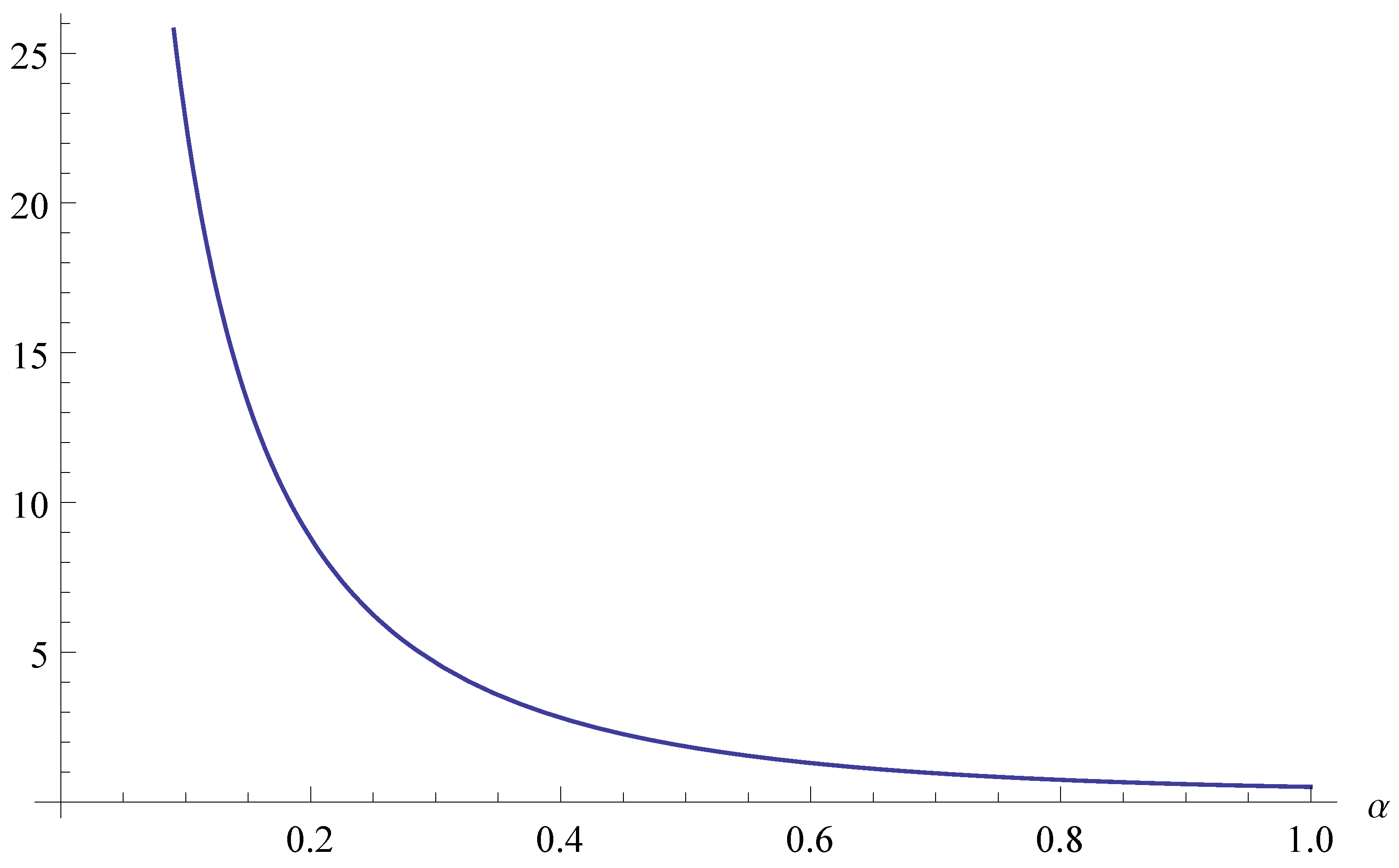
Corollary 3. Let be an infinite set of primes with positive Frobenius density that satisfies . For any even number, d, let . Assume that:Then, there are infinitely many n for which n and are simultaneously square-free numbers with prime factors all in .
We have plotted the right-hand side of the inequality against
α to illustrate the conditions under which one can obtain a twin prime-type result (
Figure 1).
Figure 1.
The right-hand side of Corollary 3 vs. α.
Figure 1.
The right-hand side of Corollary 3 vs. α.
As another sample application of our theorem, we consider the problem of representing square-free integers by translates of tuples. This problem was actually answered by Hall [
14], who even obtained an asymptotic expression for the number of such representations, but, by taking the limit,
, in Theorem 2.1, we easily obtain the following corollary.
Corollary 4. Let be an admissible k-tuple. Then, there are infinitely many n, such that all of the are simultaneously square-free.
Here, we recall from [
1] that a
k-tuple of integers is
admissible if for all prime,
p, they do not cover all the residue classes modulo
p. We remark that admissibility is not a necessary condition for this corollary to hold, but it is a natural limit of our method.
2.1. The Level of Distribution of Numbers
In this section, we will prove a Bombieri–Vinogradov-type result for
numbers if
satisfies
, generalizing a result of Orr [
15]. More precisely, we shall show that the
numbers have a level of distribution
. We remark that a set,
, with positive Frobenius density satisfies
for some
M as a consequence of Lemma 3.1 in [
7].
Lemma 1. Suppose that satisfies for some M. Then, for each b coprime to M and for any C, there exists some , such that:Proof. The result is a variant of Motohashi [
16]. Similar results are also treated by Bombieri, Friedlander and Iwaniec [
17]. We will use the modern treatment given by ([
18] (Theorem 17.4)), following the approach of Thorne ([
7] (Lemma 3.2)).
Let
be the characteristic function of
numbers congruent to
b modulo
M and
be the characteristic function of primes in
congruent to
b modulo
M. We further define
. Borrowing the notation from [
18], given an arithmetic function,
, define:
Finally, we let
denote the restriction of
to the interval,
I,
i.e.,
if
,
otherwise. We first remark that:
Hence, for
, where
will be chosen later,
Fixing
, we now split the interval
into intervals of the form
, where
. The number of such intervals is
. Then, we remark that
closely approximates
. Both functions are supported in
and identical on
. The differences on the intervals,
and
, contribute
to each
. Summing over all
and all pairs
, such that
, the total contribution of the error is:
On the other hand, we may apply Theorem 17.4 in [
18] with
and
. Note that Condition (17.13) on
β is satisfied for some
, since
satisfies the
condition, and:
where:
Hence, the theorem gives (note that
for any
):
We take
, and sum over all the pairs
, such that
to conclude that:
From there, taking
gives the desired result.
2.2. Linear Forms and Admissibility
Following [
7] and [
6], we will prove our results for
k-tuples of linear forms:
We will prove that for any admissible
k-tuple with
k sufficiently large, there are infinitely many
x for which several
simultaneously represent square-free numbers with all prime factors in
. The basic setup is the same as [
7]. We shall recall only the important notions and hypotheses in this section and refer our readers to ([
7] (
Section 2.2]) and ([
6] (
Section 3)) for a detailed exposition. As in [
7] and [
6], we define the quantities:
We recall from [
7] the following admissibility constraint.
Definition 1. Given a positive integer, M, a k-tuple of linear forms is M-admissible if the following conditions hold simultaneously.- (i)
For every prime, p, there exists an integer, , such that ;
- (ii)
for each i, M divides ;
- (iii)
for each i, M is coprime to .
A k-tuple of linear forms, , is called admissible if it satisfies only (i). The above stronger admissibility constraint is introduced to incorporate the fact that may fail to be well-distributed modulo M.
We will primarily consider the case when
. Given a set of linear forms
with
, remove finitely many primes from
, so that
for all
. Throughout the paper, we shall use
for a sum over all the values relatively prime to
A and any prime
(this is different from [
7], which only requires the values to be relatively prime to
A). As in [
7] and [
6], we may assume without loss of generality that
M-admissibility can be replaced by a stronger condition, which we label
Hypothesis . The justification for this hypothesis appears in [
7].
Hypothesis . is an M-admissible k-tuple of linear forms. The functions have integer coefficients with . Each of the coefficients, , is divisible by the same set of primes, none of which divides any of the . If , then any prime factor of divides each of the .
2.3. Preliminary Lemmas
In this section, we shall provide the setup of the proof of the main theorem and prove a few key lemmas. We first recall a lemma from [
6], which we shall use frequently in this section.
Lemma 2. ([6] (Lemma 4)) Suppose that γ is a multiplicative function, and suppose that there are positive real numbers , such that:and:if . Let g be the multiplicative function defined by:Let:Assume that is a piecewise differentiable function. Then:where: . The constant implied by “O” may depend on and κ, but it is independent of L and F. Following the approach in [
7] and [
6], we shall consider the sum:
where
are real numbers to be described later. As in [
7] and [
6], Theorem 2 will follow from the positivity of the sum,
S.
Note that there is a key distinction between our definition of
S and the definition in [
7] and [
6]. Here, we sum up
over only the square-free numbers,
d, that are relatively prime to all the primes in
. Intuitively, this gives a bigger sieve weight to the values,
n, where
has many prime factors in
; hence, the positivity of
S can be satisfied for smaller
k. As we can see in the proof of Lemma 4, this change also simplifies the calculation of
S.
For each square-free number,
d, let:
The sieve weights,
, are related to the quantities,
, by:
Then, by Möbius inversion, we have:
Since the sum of
is taken over all the square-free numbers relatively prime to the primes in
, we take
to be supported only on integers coprime to
, which implies that the
are also supported on integers coprime to
.
To determine
S, we break the sum into parts and evaluate each of them individually. Let:
Then:
We shall now estimate
and
in the following two lemmas.
Lemma 3. Suppose that is a set of linear forms satisfying Hypothesis . There is a constant, C, such that if , then:Proof. From the definition of
, we have:
where for each square-free
d with
and
for all
,
As in the proof of Theorem 7 in [
6], note that the error term is
if
. For the main term,
We use Lemma 2 with:
and
. Then,
. It can verified as in ([
6] (Lemma 7)) that the conditions in Lemma 2 are satisfied with
, using the fact that the Frobenius density of
is
. Then, the main term becomes:
with the desired error term. The result follows by evaluating the integral. ☐
Remark 4. This argument breaks down when , since κ needs to be positive in order to apply Lemma 2. A similar phenomenon occurs in the proof of Lemma 4.
Lemma 4. Let be a set of linear forms satisfying Hypothesis . There is a constant, C, such that if , then:where:and satisfies: Remark 5. The ratio,
, approaches a positive constant as
N tends to infinity by Theorem 2.4 in [
13].
Proof. From the definition of
, we have:
We remark that in the second equality, we have used the condition that
is not divisible by any prime in
, and hence, the condition
in the sum implies that
for nonzero
. This contributes to the much simpler estimate of
than that in [
7].
Let
denote the set of residue classes,
a, modulo
x, such that
. Note that
by Hypothesis
(
cf. (4.4) in [
7]). Then:
Write
, then
, with
and
. By assumption, the values,
, are all coprime. Let
. Then, we may use the Chinese Remainder Theorem to combine the congruence conditions modulo
and
into a single condition on
. Let
denote the set of all possible residue classes of
modulo
x. Then:
Now, we decompose the inner sum:
Accordingly, we can decompose
into its main term and error term
. Let
The error term can be estimated using Lemma 1 and Cauchy’s inequality as in the proof of Lemma 4.1 in [
7]. Let
, then
. Note that
. Moreover, by Hypothesis
, we have
for all
. Hence:
for any
U. To obtain the third line, we use the fact that
by (4.3) of [
6]. For the main term of
,
where
is the density of the elements congruent to
mod
M in the set of
numbers.
Our next step is to evaluate the last sum. Let
and
. Then:
by an analogue of Lemma 6 in [
6], where:
Thus:
We use Lemma 2 with:
and
. Again, the conditions are verified as in ([
6] (Lemma 7)) with
, giving:
Hence for square-free
r with
and
for all
,
Thus:
We evaluate the last sum using Lemma 2, taking
and:
The conditions are satisfied when
, as verified in ([
6] [Lemma 8]). Then:
Hence:
Plugging the definition of
and this identity into (
1), we have the desired result. Note that here we have used the fact that
by Hypothesis
.
2.4. Proof of Theorems 1 and 2
Proof of Theorem 2. Let
, where
C is the constant in Lemma 2.6. Noting that
, we have, as
,
where:
Hence,
S is positive for all large enough
N if:
where:
and:
is the beta function. Finally, by a variant of the Tauberian theorem ([
19] (Theorem 2.4.1)), we deduce that:
where, as we recall from Lemma 4,
is the function that satisfies:
For
N large enough, the infinite product approaches one. Now, the result follows from Equation (
2). ☐
Proof of Theorem 1. To derive Theorem 1.1 from our main theorem, we consider for given k and m a set of k primes, , with the appropriate residue classes as needed. Then, forms an M-admissible k-tuple, which can be normalized to fit Hypothesis . This gives us the value, , for the constant, .

