Article

Application of Machine Learning to Cluster Analysis of Diabetes Mortality at the Municipality Level in Mexico According to Sociodemographic Factors


by
Nelva N. Almanza-Ortega
1,
Carlos Fernando Moreno-Calderon
2,
Sandra Silvia Roblero-Aguilar
3,
Rodolfo Pazos-Rangel
4,
Joaquín Pérez-Ortega
2,*,
Vanesa Landero-Nájera
5 and
Víctor Augusto Castellanos-Escamilla
3
1
Secretaría de Ciencias, Humanidades, Tecnología e Innovación, SECIHTI, Mexico City 03940, Mexico
2
Cenidet, Tecnológico Nacional de México, Cuernavaca 62490, Mexico
3
IT Tlalnepantla, Tecnológico Nacional de México, Tlalnepantla 54070, Mexico
4
IT Cd. Madero, Tecnológico Nacional de México, Madero 89440, Mexico
5
Computer Systems, Universidad Politécnica de Apodaca, Apodaca 66600, Mexico
*
Author to whom correspondence should be addressed.
Mathematics 2026, 14(3), 573; https://doi.org/10.3390/math14030573
Submission received: 19 December 2025 / Revised: 22 January 2026 / Accepted: 27 January 2026 / Published: 5 February 2026

Abstract

In recent years, the mortality due to diabetes has increased around the world. In particular, diabetes is the second leading cause of mortality in Mexico, with a heterogeneous distribution of mortality rates at the municipality level. The objective of this study is the analysis of clusters of municipalities with similar values for sociodemographic indices and diabetes mortality. In this sense, an application is presented that was developed using a data science methodology and a machine learning algorithm called fuzzy c-means. For this research, 4,604,360 death certificates from 2019 to 2023 were assessed, among other official data. As a result of the analysis, two key indicators related to diabetes mortality were found, i.e., one is the percentage of population in poverty and the other is population density. The main results of this research are as follows: a direct correlation was found between population density and mortality, and an inverse correlation was found between population in poverty and mortality. In the study interval, it was observed that the cluster with less mortality showed an increase in mortality rate year after year. Finally, we consider that the tendencies found can be useful to public health authorities for optimizing the distribution of resources for treating diabetes and reducing diabetes-related mortality.
MSC:
62H30; 90C70; 68W40; 91C20; 62P10

1. Introduction

Diabetes mellitus is a chronic metabolic disease characterized by the presence hyperglycemia, i.e., high levels of glucose in blood [1]. According to the World Health Organization, the number of people that live with diabetes increased from 200 million in 1990 to 830 million in 2022. According to the International Diabetes Federation (IDF) Atlas 2025 [2], 11.1% of the adult population between 20 and 79 years of age has diabetes, i.e., approximately 1 in 9 people. From this percentage of the population, more than 40% has not been diagnosed. Projections for 2050 indicate that 1 in 8 people, approximately 853 million people globally, will live with diabetes, which amounts to an increase of 46%. In the Americas, according to the recent data from the Pan American Health Organization, in 2021, diabetes was the sixth leading cause of mortality with a mortality rate of 29.3 deaths per 100,000 people [3].
In particular, in Mexico in 2021, the mortality rate attributed to this disease was 76.1 deaths per 100,000 people, which places Mexico 13th worldwide in terms of diabetes [4]. In 2023, according to data from INEGI (the Mexican institute for statistics and geography), 110,059 deaths occurred due to diabetes in Mexico, making it the second leading cause of mortality [5].
Diabetes constitutes a public health problem that is ever more important in Mexico due to its high morbidity and mortality [6,7,8], as well as the high expenditure associated with its prevention and treatment. To obtain an idea of this expenditure in Mexico, it is important to mention that PROFECO (the Mexican consumer protection agency) published that, in 2021, Mexico spent USD 19,946.8 million on diabetes prevention and treatment [9].
The causes of diabetes are multifactorial. Some of these causes are the structural factors of population, malnutrition, obesity, and lack of physical activity, among others [10,11]. For mitigating the effect of this disease, it is known that several strategies have been implemented, which are oriented toward disease prevention and universal access to its treatment in several countries [12].
On another issue, in recent years, with the advent of computers with larger processing and storage capacities coupled with advances in data science [13,14], artificial intelligence [15,16], and particularly machine learning [17,18,19], it has been possible to address ever more complex health problems.
To date, it is known that there exist official large databases and repositories that can be processed to find new patterns about diabetes and to generate new knowledge that can be useful for public health authorities. In this sense, in this research, people mortality databases and population censuses, among others, were processed using fuzzy clustering algorithms, which allow generating new knowledge capable of helping decision making. In particular, the regions of Mexican municipalities with the highest mortality rates were determined as well as the regions with the lowest rates.
In the following three subsections, investigations that use machine learning techniques or algorithms for data processing aiming at obtaining new knowledge on diabetes are presented. The first subsection presents computer applications that use an epidemiological perspective and process data from Mexico. The second subsection differs from the first subsection as in its data from other countries are used. Finally, the third subsection describes machine learning applications that do not have an epidemiological perspective. Noteworthily, in all the research works, relevant information such as publication year, the source of data used, the machine learning techniques or algorithms employed, and the main findings reported are mentioned.

1.1. Computational Applications in Mexico Using Diabetes Data from an Epidemiological Perspective

To our knowledge, in Mexico, few investigations have been carried out on diabetes mortality that include spatial and time determinants from an epidemiological perspective.
Bello-Chavolla et al. [20] present a descriptive epidemiological analysis of diabetes mellitus type 2 (T2DM) mortality from 2000 to 2010. Their data sources were the General Directorate of Health Information (DGIS), INEGI, CONAPO (the Mexican population council), and ENSANUT (the Mexican survey on health and nutrition). From one of the results of this research, it was inferred that the diabetes mortality rate increased by 3.8% from 2000 to 2010. This increase was related to structural processes such as nutritional transition, an increased obesity prevalence in more than 70% of the adult population, a high consumption of ultra-processed food, and a sedentary lifestyle.
Additionally, genetic and socioeconomic factors have contributed to increasing the gap among regional diabetes mortality rates. This research also inferred that diabetes mortality was higher in the northern and central regions of the country. In particular, the federal entity Mexico City (denoted by CDMX) had a rate almost 30 points above the national average, followed by the state of Coahuila. In contrast, the states with the lowest mortality rates were Quintana Roo, Chiapas, and Baja California Sur.
Pérez-Ortega et al. [14] developed a Support Vector Regression model for predicting diabetes mortality in CDMX and the State of Mexico in the interval of 2020–2024. For the application development, they used the Batch MFCD methodology from data science [21]. In the experiments, they used the official mortality data from DGIS as well as population databases from INEGI and CONAPO, corresponding to the period of 1990–2019. Thus, a decreasing tendency of 10.7% was observed in the mortality rate in CDMX in the interval of 2017–2019. Additionally, for the period 2020–2024, it was projected that diabetes mortality would continue decreasing at a similar rate. The authors mentioned that year 2020 was an atypical case because of the COVID-19 pandemic; therefore, it is foreseeable that its effects will alter the actual diabetes mortality rates in the subsequent years.
Bello-Chavolla et al. [22] used spatial and negative binomial regression models and spatial autocorrelation, including Moran I and Getis-Ord Gi* statistics, for analyzing the diabetes mortality distribution at the state level and its relation to sociodemographic factors. The analysis compared the mortality rates observed in 2020 with the average mortality rates of the time period 2017–2019 using the official data from ENSANUT, INEGI, and CONAPO. For assessing the effect of sociodemographic inequalities on diabetes mortality at the national level, the social lag index (SLI) and the density-independent SLI were used. The results showed an increase in diabetes mortality rate of 41.6% in 2020 compared to the average mortality rate of 2017–2019. The states with the highest mortality rates, adjusted for age, were the State of Mexico, Tlaxcala, and Tabasco. The authors concluded that structural inequalities and the interruption of medical care during the COVID-19 pandemic resulted in the increase in diabetes mortality in Mexico.
Cervantes and Baptista [23] analyzed the spatial distribution of type 2 diabetes mortality in the 2469 municipalities of Mexico in 2020. Using mortality data from INEGI (ICD-10 codes E110–E119) and population projections from CONAPO, a hierarchical Bayesian model was applied using the INLA inference for estimating the standardized mortality ratios (SMRs) and subsequent relative risk, distinguished by age groups. The results make the central area of Mexico to stand out (CDMX, Tlaxcala, the State of Mexico, Hidalgo, and Puebla) because of its higher diabetes mortality rate in people older than 50 years. The Yucatan peninsula area (Yucatan, Campeche, and Quintana Roo) and the southeast zone of the country (Chiapas and Tabasco) show a high mortality risk due to diabetes in the population younger than 50 years. Associations between a high mortality risk and conditions such as a low education level, unsteady nutrition, and poverty were identified, whereas a larger GNP per capita was found to be associated with a lower mortality risk.

1.2. Computational Applications on Diabetes Datasets from a Global Epidemiological Perspective

Globally, diabetes research has evolved and has approaches that include spatial and sociodemographic dimensions aiming at understanding the territorial distribution of the disease and associated determinants.
In North America, relevant investigations have been carried out. In Winnipeg, Canada, Green et al. [24] performed a geographical analysis of diabetes prevalence using administrative health record sources and applying spatial scanning techniques and regression models. The results revealed significant clusters in areas characterized by unfavorable socioeconomic conditions, less healthy environments, and inadequate lifestyles, emphasizing the influence of structural factors and intra-urban heterogeneity on the disease. In Boston, Link and McKinlay [25] used logistic regression and the chi-square test to analyze disparities according to race, socioeconomic status, and medical insurance and determined education and income to be the key social determinants.
Additionally, in North Carolina, Bravo et al. [26] utilized spatial Bayesian models using the health electronic records of 41,203 people (2007–2011) as a data source for evaluating racial differences, which revealed a larger prevalence of diabetes in the non-Hispanic black population, and emphasizing the importance of built environments for understanding geographic disparities. A national research by Fang et al. [27] applied statistical methods such as linear regression, logistic regression, and ponderation for relating diabetes to sociodemographic characteristics, physical indicators, and life habits, which revealed body mass to be the most strongly associated with diabetes.
In South America, the spatial patterns of diabetes linked to social inequalities have been identified. In Chile, Crespo et al. [28] used self-organizing maps (SOMs) for clustering zones according to socioeconomic variables and found that a high diabetes prevalence is associated with low income and a low educational level. In Colombia, Montoya-Betancur et al. [29] performed an ecological study by applying the Bayesian hierarchical model smoothing and LISA statistic for identifying the persistent clusters of type 2 diabetes mortality (2003–2016), and they unexpectedly found a positive association between mortality and economic development. In Brazil, Oliveira et al. [30] used a Bernoulli model for finding the clusters in zones with a low educational level and low income, and the areas with high levels of both education and income showed a low diabetes prevalence.
In Asia, investigations have been carried out mainly in India and China. In India, Valson et al. [31] applied the Bernoulli model for discovering the clusters of high and low prevalence; in contrast, population density did not show a significant association with diabetes mortality, while factors such as criminality and traffic accidents did show an association. In China, investigations have found significant results twice. First, Zhou et al. [32] conducted a national analysis that involved 161 districts between 2006 and 2012 by applying multilevel negative binomial models with data sources from the China Mortality Surveillance System. Their results showed a general reduction of 12% in diabetes mortality rates with decreases in urban areas larger than those in rural areas, though regional inequalities persisted, i.e., the northwestern and northeastern regions showed a significantly higher diabetes mortality risk than the southern region. Mortality was associated with larger urbanization, body mass index, and high temperatures, while factors like smoking, cholesterol level, and the local prevalence of diabetes did not show any significant relations.
Finally, Luo et al. [33] performed a spatial temporal analysis of diabetes mortality in the Guangdong province, aiming to identify high-risk areas and its socio-environmental determinants. By using the empirical Bayesian kriging techniques and spatial Poisson scanning, critical mortality clusters were identified mainly in the eastern and western coastal zones of the province, with a significantly higher relative diabetes mortality risk than that of other regions. The authors found that exposure to atmospheric contaminants, especially carbon monoxide, was significantly associated with high mortality risk. In particular, the mortality results from this research, similar to ours, suggest that, in densely populated areas, as the population’s income increases, the mortality rate increases.

1.3. Application of Machine Learning to Diabetes Datasets

To date, it is known that investigations that aimed to find new knowledge about diabetes from the analysis of datasets about the disease have successfully used machine learning techniques. In general, diabetes research follows an epidemiological or clinical approach, and the source data have the same nature. As mentioned before, the current article follows an epidemiological approach. However, to get an idea of other machine learning applications that are mainly clinically orientated, several relevant applications will be briefly described. The readers that wish to delve further into machine learning applications on diabetes can read articles [34,35,36], since they include systematical surveys. In the rest of this subsection, investigations that use supervised learning techniques are mentioned, followed by non-supervised learning techniques.
Some examples of investigations that used supervised learning are described next. Prabhu et al. [37] used Deep Belief Networks with the Pima Indians diabetes dataset. Elmenshawy et al. [38] integrated models such as XGBoost with explicable artificial intelligence (XAI) (SHAP and LIME), allowing the generation of comprehensive predictions from the clinical data of Bangladeshi female patients. Allani et al. [39] developed an interactive platform based on LightGBM with local explainability (SHAP and LIME) applied to the BRFSS 2015 dataset. Complementarily, Olaniran et al. [40] proposed a hybrid approach that combines the random selection of characteristics and LSTM/BiLSTM networks, which was evaluated using three datasets: the Pima Indians diabetes dataset, the diabetic retinopathy Debrecen dataset, and the early-stage diabetes risk prediction dataset.
The recognition of diabetes subtypes has also been approached by using supervised models. Omar et al. [41] used neural networks to classify four Mexican clinical cohorts: SIGMA, Metabolic Syndrome, ENSANUT 2016, and CAIPaDi. From their results, four consistent clinical subgroups were found, i.e., SIDD, SIRD, MOD, and MARD. Tanabe et al. [42] used Random Forest for classifying four subtypes, using data from two Japanese clinical cohorts. Antonio-Villa et al. [43] carried out a transversal analysis by using data from ENSANUT 2016, 2018, and 2020–2022. Additionally, by using self-normalizing neural networks (SNNNs), 23,354 adults were classified into four subgroups of type 2 diabetes (MOD, SIDD, SIRD, and MARD). Taurbekova et al. [44] validated five subtypes of diabetes by conducting a cross-sectional review and study on a sample of 558 patients. Preedasawakul et al. [45] proposed the 4TaStiC algorithm, which was tested using HbA1c (a measure of average blood sugar) time series data of 1989 patients with diabetes for clustering patients based on both HbA1c levels and hidden trends and patterns.
Described next are some applications that used unsupervised learning. Carrillo-Larco et al. [46] used k-means on national health surveys in Latin America and the Caribbean with data from 8361 adults, which revealed four population profiles. Manzani et al. [47] analyzed the clinical trajectories from 11,028 patients with diabetes by using a Kernelized-AutoEncoder, which revealed seven clinically relevant evolution clusters. Abbasi et al. [48] used the k-prototype clustering algorithm on pediatric records and found five clinical diabetes subtypes with a risk of complication. Finally, Priambodo et al. [49] evaluated lifestyle factors associated with the diabetes risk by using the k-means algorithm on a dataset of 912 patients of Puskesmas Jayanti (a community health center) in Indonesia.
Most of the machine learning applications regarding diabetes have been developed from hospital datasets, which utilize individual clinical variables. In contrast, this research proposes a different approach, based on population mortality datasets, to analyze groups related to diabetes mortality rates at the municipality level by applying a machine learning algorithm and data science from an epidemiological perspective.
The remaining article is organized as follows: Section 2 describes the first four steps of the approach used. Section 3 addresses the remaining two steps by integrating them as a part of the analysis of results and discussion. Finally, Section 3 presents the conclusions.

2. Methodology

In this research, the methodology known as Batch MFCD [14] was utilized, a variant of the one developed by IBM [21]. This methodology has been previously applied in studies related to the COVID-19 mortality rate in Mexico from an epidemiological perspective [13]. This methodology is illustrated in Figure 1 and consists of six steps: (1) business understanding, in which the research questions are defined; (2) data collection, in which the gathering of datasets from different sources is carried out; (3) data preparation, in which the selection of attributes and records from the obtained databases is performed, new attributes are generated from calculating the initial attributes, and the values of the new attributes are normalized for a better interpretation of the results; (4) modeling, in which a clustering model is selected; and the steps 5 and 6 are not described in separate subsections, since graphic displays were used in Section 3 for facilitating the reading and interpretation of results.

2.1. Business Understanding

According to the principles of data science [50], the formulation of objectives and the research question must be presented in the initial steps of the project. Therefore, the questions that oriented this project were as follows: (1) what are the clusters of Mexican municipalities with high diabetes mortality rates according to sociodemographic factors? and (2) what are the time patterns of mortality rates of clusters in the interval 2019–2023?
In the context of this research, it is important to mention that Mexico is divided into 31 states and CDMX; in turn, states are divided into municipalities except CDMX, which is subdivided into districts. To facilitate comprehension, in the rest of this article we will use the term municipality for the CDMX districts.

2.2. Data Collection

In this step, the attribute values are selected and prepared for their use in the modeling and evaluation. In this study, records from four official datasets from Mexico were obtained, which are described in Table 1.

2.3. Data Preparation

2.3.1. Selection of Attributes

This section describes the attributes that were selected for creating the data warehouse. The data warehouse attributes are of two types: one involving attribute directly selected from the datasets, which are called base attributes, and the other including indicators.
Noteworthily, numerous experiments were carried out with different combinations of attributes of different datasets without obtaining conclusive results. Therefore, the grouping of the combinations of base attributes and indicators was attempted. Satisfactory results were obtained with this approach, as described in Section 3.
Table 2 shows the base attributes selected from each dataset. The next subsection shows the process for calculating the indicators.

2.3.2. Generation of Indicators

This subsubsection describes the procedure used for calculating indicators for the municipality level, which were crucial for carrying out this research. The first indicator was the population density at the municipality level, and the second indicator was the mortality rate at the municipality level per 100,000 inhabitants.
Population   density = Population km 2
Mortality   rate = Deaths Population     ×     100 , 000

2.3.3. Record Selection

Noteworthily, in this research, only municipalities with a population greater than 100,000 inhabitants were considered. A total of 234 municipalities that met this criterion were included, since those with a smaller population could introduce biases in the interpretation of results.
Mortality records were selected according to the values of the mortality cause attribute. In particular, the values were those in the interval E10 to E14 and those in E232, O240, O241, O244, P700, and P702. These values are related to disease codes associated with diabetes, according to the International Statistical Classification of Diseases and Related Health Problems 10th Revision [56].

2.3.4. Normalization of Attribute Values

The values of population density and percentage of people in poverty attributes were normalized. Equation (3) shows, in a general way, the calculation for normalizing a set X of attribute values.
x = x x m i n x m a x x m i n
where x′ denotes the normalized value of x; the largest value of the set of values is xmax, and the smallest is xmin.

2.4. Modeling

For selecting the clustering algorithm, several exploratory experiments were performed using the following algorithms: standard k-means [57], k-means++ [58], standard fuzzy c-means (FCM) [59], and a hybrid variant called fuzzy c-means++ (FCM++) [60]. As a result of these experiments, it was found that FCM++ was the algorithm that obtained better solutions for our specific application; therefore, it was selected for use in the rest of the investigation. The FCM++ variant differs from the standard FCM algorithm as it uses the k-means++ algorithm for generating the initial centroids.
In the rest of this section, the k-means++ and FCM algorithms are described, and their respective pseudocodes are shown.

2.4.1. Algorithm k-Means++

Algorithm k-means++, proposed in [58], initializes the cluster centroids of the k-means algorithm by randomly selecting objects from the set of data as explained next. First, let D(x) be the shortest distance from a point x to the closest centroid that has already been chosen. Next, randomly choose the initial centroid v1. Main step: determine the next centroid by choosing viX with probability D(vi)2/∑xX D(x)2. Finally, repeat the main step until k centroids are determined. The pseudocode of algorithm k-means++ is shown in Algorithm 1.
Algorithm 1: k-means++
1Initialization:
2      X: = {x1, …, xn}; //The set of data
3      Assign the value for k;
4      V: = {}; //The set of centroids is initialized
5      V: = V U {vi}; //Where the first centroid vi is selected randomly
6      for i = 2 to k do
7            Select the i-th centroid viX that maximizes probability D(vi)2/∑xX D(x)2;
8            V: = V U {vi};
9       end for
10      Return V;
11End of algorithm
Algorithm 1 shows the initialization of centroids by using the algorithm k-means++. Given the dataset X and the number of clusters k, the first step consists of selecting the first centroid v1 randomly from the dataset X (line 5). Next, v1 is incorporated to the set of centroids denoted by V (line 5). Finally, for the second centroid and until the number of centroids equals k, the i-th centroid must be selected to maximize a probability distribution across all values of xX (lines 6 to 9).

2.4.2. FCM Algorithm

The clustering algorithm FCM [59,61] is a fuzzy-type partitional algorithm. The algorithm is based on an objective function, which is shown in Equation (4).
J m ( U , V ) = i = 1 n j = 1 c u i j m x i v j 2
where U = uij denotes the membership degree of each object i to each cluster j; V = {v1,…,vc} denotes the set of centroids, where vj represents the centroid of cluster j; m denotes the weighting exponent or fuzzy factor, which represents the membership degree m > 1; c denotes the number of clusters; n denotes the number of objects; and ‖xivj2 denotes the Euclidean norm.
The solution of the clustering of dataset X is defined by the (U, V) pairs, which minimize the value of Jm.
In the convergence process, the algorithm uses Equations (5) and (6).
u i j = 1 k = 1 c x i v j 2 x i v k 2 1 m 1
v j = i = 1 n u i j m x i i = 1 n u i j m
where xi and vj are vectors in the R d space and are defined by Equations (7) and (8).
x i = ( x 1 , x 2 , , x d )
v j = ( v 1 , v 2 , , v d )
The restrictions of fuzzy clusters are presented in Equations (9)–(12).
u i j [ 0 , 1 ]
j = 1 c u i j = 1
u i j = 1   if   x i = v j
0 < i = 1 n u i j < n
Equation (9) affirms that the membership degree of any object i to cluster j must lie in the interval from 0 to 1. Equation (10) shows that the membership degree of object i to all the clusters must be 1. Equation (11) indicates that the membership degree of object i to cluster j is 1 if the object xi is at the same position as centroid vj. Equation (12) affirms that the sum of all the membership degrees of objects to a cluster must be larger than 0 and smaller than n, i.e., there cannot be empty clusters or clusters with zero objects.
The pseudocode of the FCM algorithm is shown in Algorithm 2. The K++ function is called in line 4, which generates the initial centroids V′. In the rest of this article, this variant of FCM is called FCM++.
Algorithm 2: Fuzzy C-Means++
Input: dataset X, c, m, t, ε
Output: V, U
    1Initialization:
    2          X: = {x1, …, xn};
    3          c: = 20;
    4          Function K++ (X, c);
    5                    Return V′;
    6          m: = 1.3;
    7          ε: = 0.01;
    8          t: = 0;
    9Calculate membership matrix U(0):
    10          Calculate the membership matrix using Equation (5);
    11Repeat
    12           Calculate centroids:
    13                    Calculate the centroids using Equation (6);
    14          t: = t + 1;
    15           Calculate membership matrix U(t):
    16          Calculate the membership matrix using Equation (5);
    17Until |U(t)U(t−1)| < ε
    18End of algorithm

3. Experimental Results and Discussion

This section is subdivided into four parts: the experiment design, result analysis, analysis of time pattern results, and their discussion.

3.1. Experiments Design

In this subsection, the experiments carried out and their parameters are described. For each year of the study interval (2019–2023), the clustering of municipalities with similar values of population density and percentage of population in poverty was carried out using the FCM++ algorithm. In the five experiments, corresponding to each year of the study, the values of used parameters were as follows: c = 20, m = 1.3, and ε = 0.01.
In particular, the value of c was selected based on a series of experiments conducted using the different values of c. For each clustering configuration, the partition coefficient, partition entropy, and silhouette index were computed. As shown in Table 3, the best results were obtained for c = 20 across all three indices.
The datasets from the years 2019 to 2023 were clustered using the initial centroids of the dataset from the year 2019. These centroids were generated using the K++ function of the initialization phase of algorithm FCM++. However, for the datasets from 2020 to 2023, the K++ function was omitted in the initialization, and the centroids calculated for the dataset from 2019 were used instead.
The FCM++ algorithm was implemented in C language using the GCC 7.4.0 compiler. The computational experimentation was carried out on an Acer Nitro 5 computer with a Windows 11 operating system Intel® Core™ i7-11800H processor at 2.30 GHz with 16 GB of RAM memory, 512 GB SSD, and 1 TB HDD. Python 3.12 was used with the Matplotlib 3.10 library for drawing scatter plot graphs, and the Cartopy 0.24 library was used for drawing map graphs. The R version 4.4.1 development environment was used for calculating the Pearson correlation.

3.2. Result Analysis

In this subsection, the results of the five experiments carried out are presented. Table 4 shows the results of the clustering of the dataset for 2020. The first column shows the cluster identifier, the second and third columns show the centroid values of the population density and percentage of population in poverty attributes, the fourth column shows the number of municipalities that belong to the cluster, and the fifth column shows the calculated average of the mortality rate of each cluster.
Noteworthily, clusters 10, 3, and 7 have larger values of population density and average mortality rate. Cluster 19 is atypical with only one municipality, which has a similar population density value to those of clusters 3 and 7 but a larger population in poverty value. This cluster has smaller mortality rate values. Additionally, cluster 11, which has the smallest value of population density, has also the smallest average mortality rate. In the rest of this article, clusters 10, 3, 7, and 11 are called clusters of interest, since they have the most extreme values of average mortality rate and are particularly important for this research.
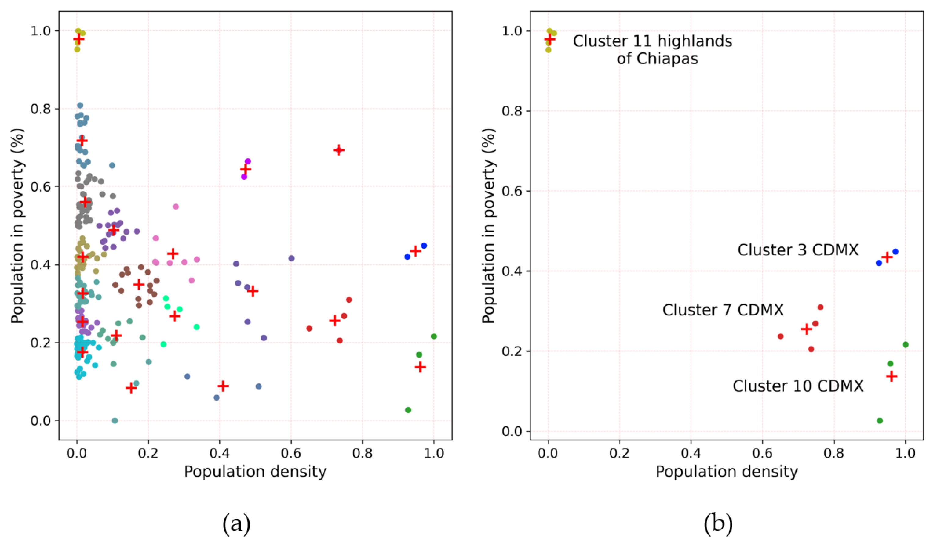
Table 4 shows both a high mortality rate and a high population density. However, the mortality rate is low when the percentage of population in poverty is high. For comparing the population density and percentage of population in poverty with the mortality rate, a Pearson correlation was performed. It was observed that the population density and mortality rate values have a high correlation of 0.74, while a negative correlation is observed for the poverty values. Additionally, the average age of people in clusters 10, 3, and 7 is 69 years, while for cluster 11, it is 59 years. Figure 2 shows the result of the clustering presented in Table 4.
In Figure 2a,b, the values on the x axis represent population density, the values on the y axis represent population in poverty and the symbol + represents the centroid of each cluster. The values of indicators are shown normalized in the interval from 0 to 1. In panel (a), the centroids of the 20 clusters are represented by crosses, and the municipalities included in this research are represented by dots. In the lower right corner, the clusters with the largest population density and the lowest population in poverty are shown, while, in the upper left corner, the cluster with the lowest population density and the largest population in poverty is shown. In panel (b), only the clusters of interest are shown.
Table 5 shows the values of the centroids of the so-called clusters of interest. The first three rows are related to clusters with a high mortality rate, which are located in the north of CDMX. The fourth row is related to the cluster with the lowest average mortality rate, which is in the State of Chiapas.
Table 5 presents the information on clusters of interest and the changes that the mortality rate has experienced over the years. The first column has the rows for the years 2020 and 2001 highlighted in red to emphasize the span of the COVID-19 pandemic. Clusters 10, 3, and 7 are the clusters with a high mortality rate located in the north of CDMX. Additionally, the ages of people that died are 68 to 70 years old. Cluster 11 has the smallest average age at death, which is located in Chiapas. Furthermore, the ages of people that die are smaller: 63 to 64 years on average. Table 6 presents the names of the municipalities that are members of each cluster.
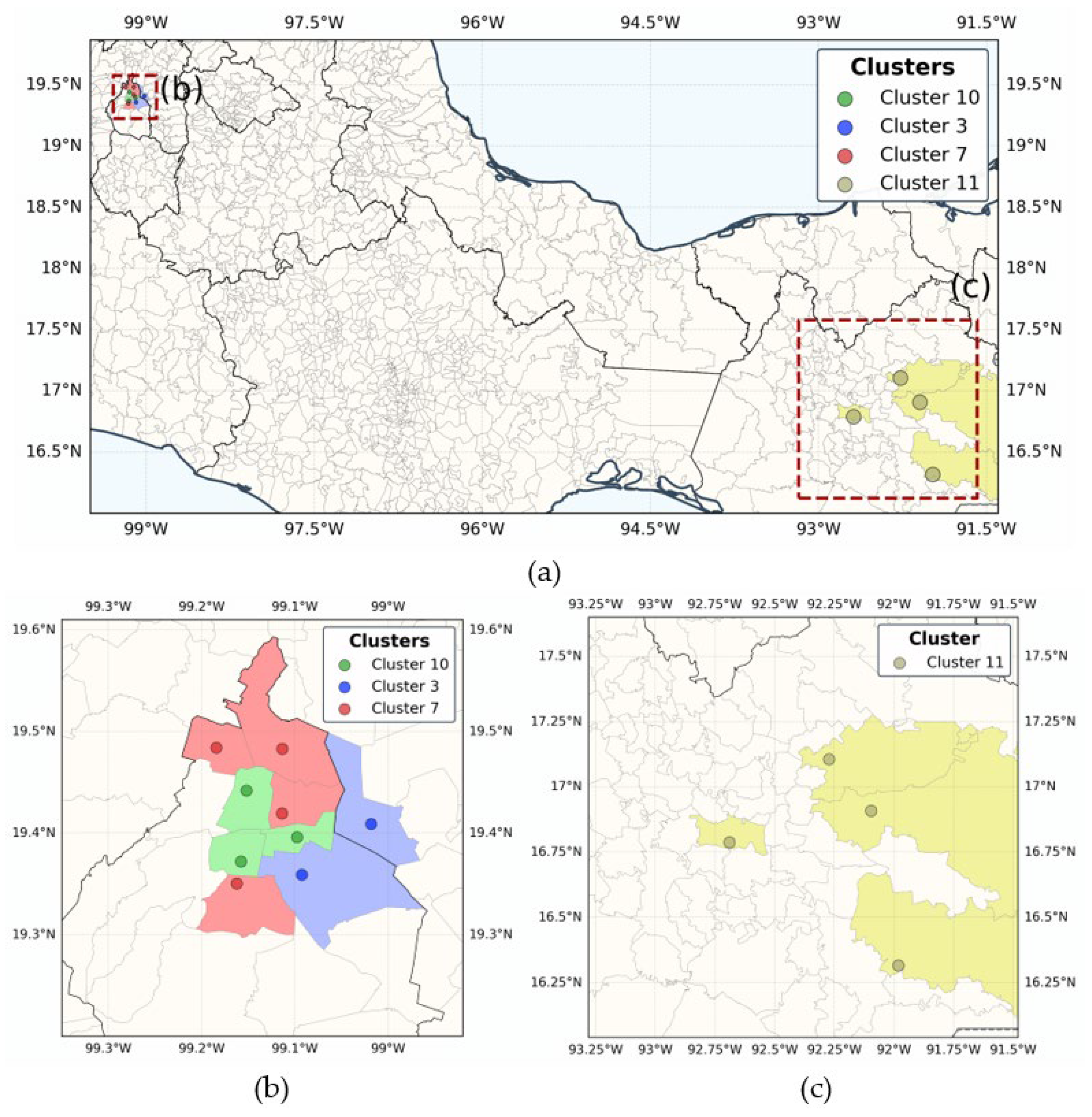
Figure 3 shows the results of municipality clustering in a geospatial plot to facilitate the interpretation of the clustering results.
Figure 3 comprises three panels. Panel (a) shows a geospatial plot of the municipalities of the clusters of interest; additionally, for the better interpretation of data, dots represent municipal seats, and each colored space symbolizes the geographical area of each municipality. Panel (b) presents a zoomed-in view of panel (a) in the CDMX area. In this area, there are three clusters whose elements are represented by colored dots. These clusters are located in the north of the city and are contiguous or close to each other. In contrast, panel (c) shows the cluster with the smallest mortality rates, which is located in Chiapas. This cluster is located in Chiapas Hights, which is inhabited by Indigenous people and a region with high poverty and marginalization in Mexico.

3.3. Analysis of the Results of Time Patterns of Clusters

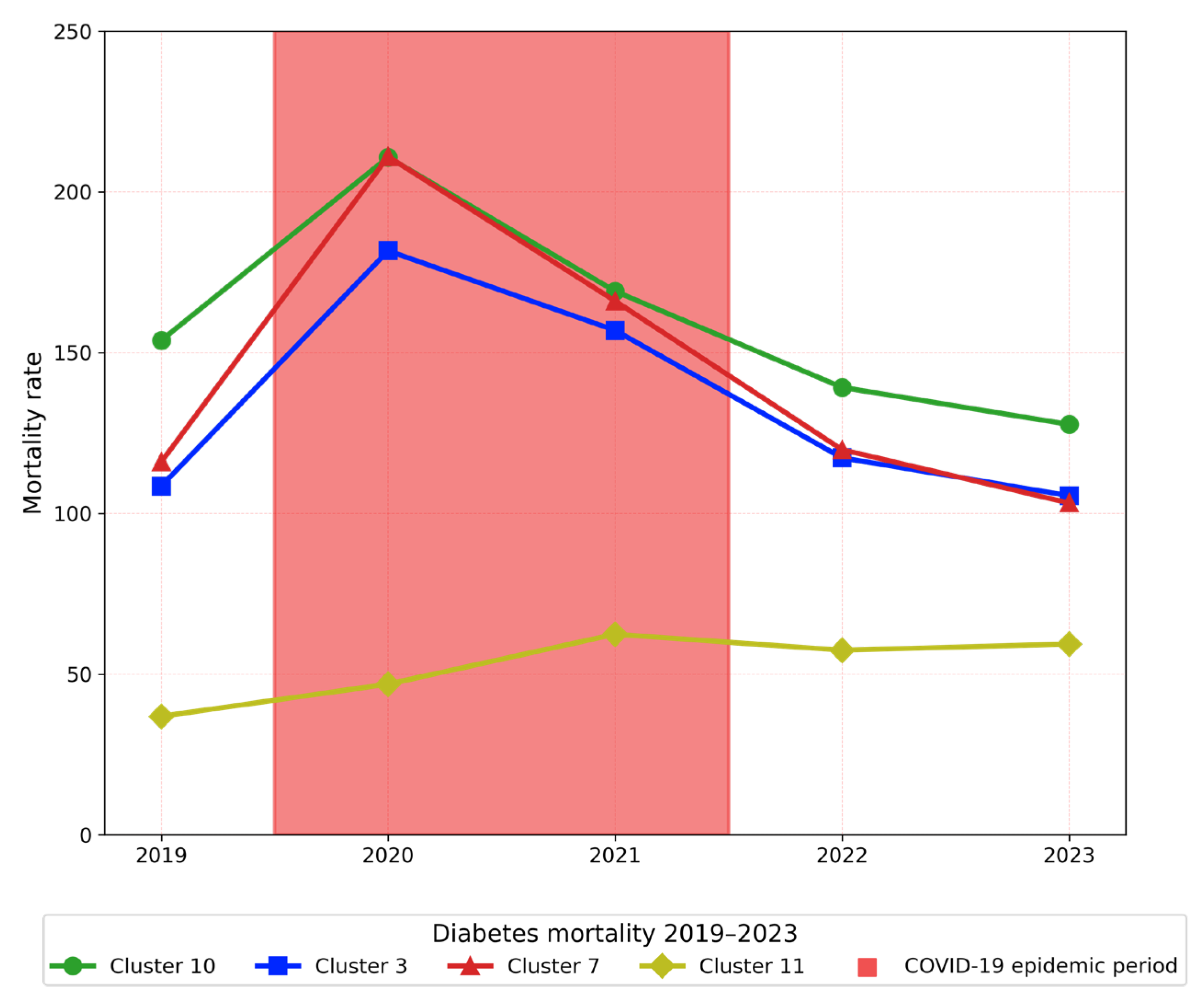
This subsection presents the analysis of time patterns of clusters through the years. Figure 4 shows the trend of mortality rate of the clusters of interest for the years 2019 to 2023.
Figure 4 shows the mortality values associated with each of the clusters of interest in the time period from 2019–2023. It is observed that clusters with the highest mortality rates, mainly located in CDMX, show a decreasing trend over time. In contrast, the cluster with the lowest mortality rate, corresponding to the Chiapas Hights, shows an increasing trend for the same indicator. Noteworthily, as they are clusters of interest, these trend results are especially relevant. In the municipalities of CDMX, diabetes mortality has decreased over the years in the study interval.
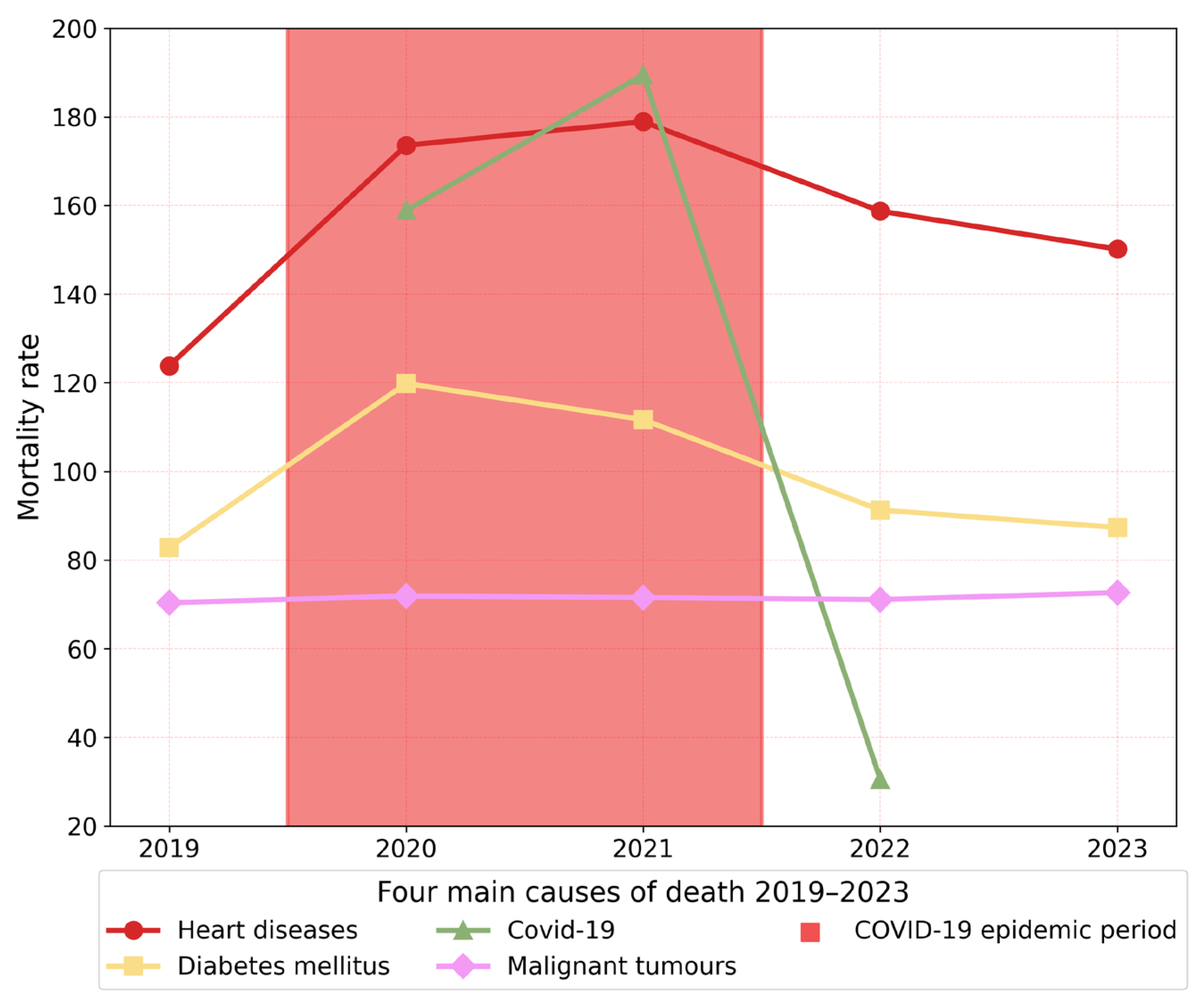
The area highlighted in red in Figure 4 represents the time period of the COVID-19 pandemic, which might be the reason for the decrease in the diabetes mortality rate of the clusters in CDMX. In contrast, for the cluster of interest located in Chiapas, mortality shows an increasing trend over the years, which suggests an increasing vulnerability in this region. In the Chiapas region, there were less deaths by COVID-19, which was a possible cause for the increase in diabetes mortality rate. Figure 5 shows the four main causes of death in Mexico from 2019–2023.
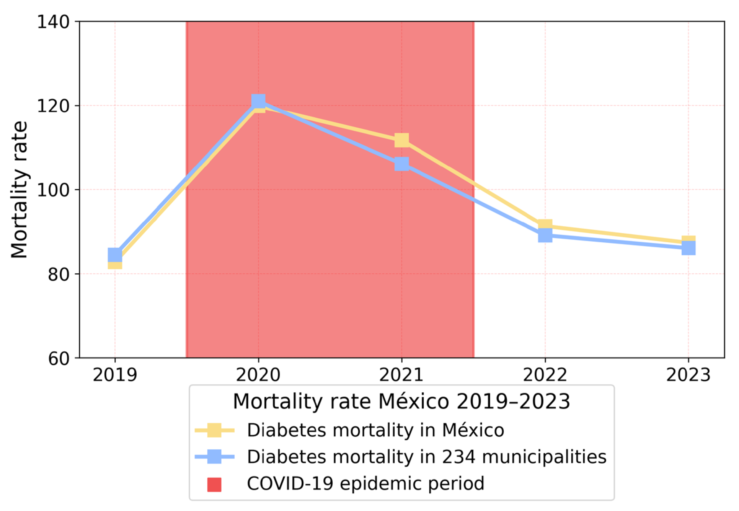
Figure 5 shows the number of deaths by heart diseases, diabetes mellitus, COVID-19, and malignant tumors. The COVID-19 pandemic started in 2020, and in the period of 2020–2021, an increase in the number of deaths due to COVID-19 occurred, while the number of deaths caused by diabetes decreased. Similar trends are observed for the causes of death due to heart diseases. However, for deaths due to malignant tumors, a slight increase was noted. The behavior of diabetes mortality rate in the entire Mexico (2478 municipalities) was compared to that of the selected 234 municipalities. Figure 6 shows the trends of both of these diabetes mortality rates.
It is evident from Figure 6 that the trends for both mortality rates are similar. The mortality rate for the 234 municipalities is larger than the nationwide mortality rate in the years 2019–2020. However, from 2021, the mortality of the 234 municipalities is smaller than that of the entire nation.

3.4. Discussion

The analysis of population databases with an epidemiological approach is complex, and the number of investigations performed in Mexico has been limited [14,20,22,23].
This problem has several dimensions. One of these dimensions is the ingress to other databases for accessing complementary information on populations, for example, census data. Another one dimension is accessing databases on the geographical and statistical information of entities or subdivisions of a country, for knowing information such as the average income of inhabitants or territorial area. Additionally, it is necessary that the data from different sources cover the same time period for the new generated knowledge to be valid. Another dimension involves the computational tools and methodologies used for the analysis. As previously mentioned, in this research, we applied machine learning techniques and a data science methodology.
The rest of this subsection contrasts the results of this research with those of other works on the following aspects: (1) cluster granularity, (2) the key parameters or variables used for clustering, and (3) the results and patterns of clustering.
Concerning granularity, in this research, clusters were defined as groups of municipalities with similar values in two sociodemographic indices. This approach provided a possible advantage over other investigations and permitted the identification of the risk patterns related to diabetes mortality with greater precision by considering structural factors, which are common to municipalities, beyond their geographical positions. In contrast, in other investigations, clusters are predefined as regions constituted by municipalities or states of a nation. For example, in reference [20], the authors divided Mexico into northern, central–western, central, and south–southeastern regions; in [23], the nation was divided into Baja California, northern Mexico, Bajio (region in central–western Mexico), Pacific coast, central Mexico, and the Yucatan peninsula; in [22], the individual states were considered for clustering; in [14], two clusters were considered, i.e., one of CDMX and the other of the State of Mexico. In investigations from other countries, clustering is performed according to different parameters [27,28,29,30,31,32].
Concerning variables, the reviewed literature shows a large diversity in the analysis of mortality and prevalence of diabetes as well as the characterization of social and spatial inequalities. In Mexico [14,20,22,23], the authors mainly used sociodemographic variables such as age, sex, educational level, and socioeconomical level as well as public health and clinical indicators such as body mass index (BMI), hypertension, glucose level, comorbidities, and excess mortality. Additionally, contextual and spatial factors were included, among which municipal marginalization, urbanization, and regional inequalities were the prominent ones.
At the international level, the investigations in [24,25,26,27] included variables related to race/ethnicity, economic income, life habits, diet, and physical activity, which allows a deeper analysis of disparities in diabetes prevalence. In Latin America [28,29,30] and Asia [31,32,33], spatial and socio-environmental indicators, such as urbanization, characteristics of the built environment, poverty, environment contamination, and access to health services, were integrated.
In contrast, in this research, only two variables were defined, i.e., percentage of population in poverty and population density as crucial for applying the FCM clustering algorithm. This methodological decision allowed us to clearly and precisely determine the municipalities with a higher diabetes mortality while avoiding information overload. Noteworthily, incorporating a larger number of variables might enrich the analysis, but it also increases the complexity of the result interpretation, since the interaction of multiple sociodemographic, clinical, and spatial factors tends to generate patterns that are more difficult to discover. Therefore, the focalized use of a small number of relevant variables guarantees an equilibrium between model robustness and the analytical clarity necessary for guiding decision making in public health.
Regarding the obtained results, previous findings show a significant spatial variability in diabetes mortality in Mexico. In [8], for the interval 2000–2010, the highest mortality rates were concentrated in the central and north regions of Mexico, with minimal rates in Quintana Roo, Chiapas, and Baja California Sur; however, these values do not reflect the recent changes in the geographic distribution of the disease. In [10], the increase in mortality occurred mainly in the southeast and east coast because of social underdevelopment, more hospitalization by COVID-19, and high prevalence of HbA1c levels of ≥7.5%. Additionally, in [12], a significant territorial heterogeneity was detected with a high mortality risk in central Mexico, the Yucatan peninsula, and southern Mexico (Oaxaca and Chiapas), which are related to a low education level, food insecurity, marginalization, and a protecting effect associated with a higher GDP per capita.
In contrast, this research found that eight municipalities in CDMX and one in the State of Mexico concentrate the highest mortality rates, though with a decreasing trend, and the cluster with the lowest mortality, located in Chiapas, has a low population density, adverse socioeconomic conditions, and an increasing trend of mortality rate in the analyzed period. This set of evidence reinforces the necessity of using up-to-date space temporal analyses for finding the recent changes in risk patterns and guiding focalized interventions that consider the socioeconomic and territorial dimensions of the disease.
As a result of this investigation, two key socioeconomic indicators are significant contributions for carrying out the clustering of diabetes mortality at the municipality level. One of these indicators is the municipal population density, and the other indicator is population in poverty at the municipality level. Noteworthily, the population density indicator showed a high correlation with the mortality rate at the municipality level. Such indicator has not been reported in other investigations on this subject, as far as the authors are aware. The indicator of population in poverty has been included in several investigations, frequently with different names or variants such as low income [28,30], economic troubles [25], low socioeconomic status [24], and GDP per capita [29,33].
In this research, as a result of clustering based on the two aforementioned indicators, three clusters located in the north of CDMX were found, which have high mortality rates, very high population densities, and very low levels of population in poverty. In other words, the higher the population income and density, the higher the mortality. Other investigations have arrived at very similar results, for example, references [29,32,33]; in particular, in [33], the authors suggest that this pattern occurs in countries or regions with medium-developed and developing areas. In contrast, other investigations have found that the higher the population income, the lower the mortality rate according to [24,25,28,30]. There is no agreement about the correlation between population income and mortality rates, thus showing the need for carrying out more complete future work that allows a better explanation of the relationship between these factors. It is foreseeable that, in order to get a better understanding of the problem, it will be necessary to include additional indicators.
Finally, we consider that the results of this study suggest that an intervention by public health authorities, focused on diabetes care in the northern area of Mexico City, would represent an important contribution to addressing diabetes due to its impact on a densely populated region of Mexico.

4. Conclusions

In this investigation, through the use of machine learning and data science, it is shown that it is possible to find regions with high or low rates of diabetes mortality as well as their trends in an interval of time. All data were obtained from official Mexican governmental sources. The main databases used were death records 2019–2023, population and housing census 2020, poverty indicators 2020, and municipal information records, which were the basis for integrating the data warehouse used by the fuzzy c-means algorithm. One of the challenges faced by this research was the selection of the attributes to be used by the clustering algorithm; therefore, several combinations of socioeconomic variables were tested, and the best results were obtained with the poverty indicator and population density at the municipal level. For this study, in order to avoid bias, only municipalities with populations greater than one hundred thousand people were included.
Through this investigation, we found that there is a high direct correlation between mortality rate and population density and an inverse correlation between mortality rate and the percentage of the population in poverty. An unexpected finding was that three regions of municipalities in the north of CDMX with very low percentages of the population in poverty had the highest mortality rates in Mexico; however, they exhibited a decreasing trend in their mortality rates in the interval from 2019–2023. The cluster with the lowest mortality rate was located in Chiapas, which had low population density and high poverty indicator; however, an increasing trend for its mortality rate was observed. Finally, we consider that the findings of this investigation can be beneficial for decision making by public health authorities regarding budget expenditure and the implementation of programs for the prevention and treatment of diabetes.

Author Contributions

Conceptualization, J.P.-O., N.N.A.-O., C.F.M.-C. and S.S.R.-A.; methodology, J.P.-O., N.N.A.-O., C.F.M.-C. and S.S.R.-A.; software, C.F.M.-C., S.S.R.-A. and V.L.-N.; validation, J.P.-O., N.N.A.-O., C.F.M.-C., S.S.R.-A., and R.P.-R.; formal analysis, J.P.-O., N.N.A.-O., R.P.-R. and V.A.C.-E.; investigation, J.P.-O., N.N.A.-O., C.F.M.-C. and S.S.R.-A.; resources, V.L.-N., V.A.C.-E. and R.P.-R.; data curation, C.F.M.-C., S.S.R.-A., V.L.-N. and V.A.C.-E.; writing—original draft preparation, J.P.-O., C.F.M.-C. and S.S.R.-A.; writing—review and editing, J.P.-O., N.N.A.-O., C.F.M.-C., S.S.R.-A., R.P.-R., V.L.-N. and V.A.C.-E.; visualization, J.P.-O., N.N.A.-O. and C.F.M.-C.; supervision, J.P.-O.; project administration, J.P.-O.; funding acquisition, J.P.-O., C.F.M.-C., S.S.R.-A., V.L.-N. and V.A.C.-E. All authors have read and agreed to the published version of the manuscript.

Funding

Carlos Fernando Moreno Calderón acknowledges his scholarship (grantee no. 1000864) from the Secretaría de Ciencia, Humanidades, Tecnología e Innovación, Secihti.

Data Availability Statement

The data presented in this study are openly available in Dirección General de Información en Salud, DGIS. http://www.dgis.salud.gob.mx/contenidos/basesdedatos/da_defunciones_gobmx.html (accessed on 30 May 2025). Instituto Nacional de Estadística y Geografía, INEGI. https://www.inegi.org.mx/app/ageeml (accessed on 30 May 2025) and https://www.inegi.org.mx/programas/ccpv/2020/#Datos_abiertos (accessed on 30 May 2025). Consejo Nacional de Evaluación de la Política de Desarrollo Social, CONEVAL. https://www.coneval.org.mx/Medicion/Paginas/Pobreza-municipio-2010-2020.aspx (accessed on 30 May 2025). Sistema Nacional de Información Municipal, SNIM. http://snim.rami.gob.mx (accessed on 30 May 2025).

Conflicts of Interest

The authors declare no conflicts of interest.

References

  1. World Health Organization. Available online: https://www.who.int/es/news-room/fact-sheets/detail/diabetes (accessed on 30 May 2025).
  2. International Diabetes Federation. Available online: https://idf.org/es/about-diabetes/diabetes-facts-figures/ (accessed on 15 June 2025).
  3. Organización Panamericana de la Salud. Available online: https://www.paho.org/es/enlace/causas-principales-mortalidad-discapacidad (accessed on 2 June 2025).
  4. World Health Organization. Available online: https://ourworldindata.org/grapher/death-rate-from-diabetes-ghe?time=latest&mapSelect=FJI~MUS~PLW~TTO~KIR~HRV~MHL~JAM~FSM~BRB~TON~TUV~MEX#sources-and-processing (accessed on 10 July 2025).
  5. Instituto Nacional de Estadística y Geografía (INEGI). Available online: https://www.inegi.org.mx/app/saladeprensa/noticia/9409 (accessed on 12 July 2025).
  6. Soto Estrada, G.; Moreno Altamirano, L.; Pahua Díaza, D. Panorama epidemiológico de México, principales causas de morbilidad y mortalidad. Rev. Fac. Med. UNAM 2016, 59, 8–22. [Google Scholar]
  7. Bragg, F.; Kuri-Morales, P.; Berumen, J.; Garcilazo-Ávila, A.; Gonzáles-Carballo, C.; Ramírez-Reyes, R.; Santacruz-Benitez, R.; Aguilar-Ramirez, D.; Gnatiuc Friedrichs, L.; Herrington, W.G.; et al. Diabetes and infectious disease mortality in Mexico City. BMJ Open Diabetes Res. Care 2023, 11, e003199. [Google Scholar] [CrossRef]
  8. Bragg, F.; Kuri-Morales, P.; Trichia, E.; Torres, J.M.; Baca, P.; Garcilazo-Ávila, A.; González-Carballo, C.; Ramirez-Reyes, R.; Rivas, F.; Aguilar-Ramirez, D.; et al. Type 2 diabetes and cause-specific mortality in Mexico City: A Mendelian randomisation analysis. Lancet Reg. Health-Am. 2025, 45, 101082. [Google Scholar] [CrossRef]
  9. Revista del Consumidor (PROFECO). Available online: https://bibliotecadelconsumidor.profeco.gob.mx/documento/68155aed350daaf0cb0cd24f (accessed on 26 January 2026).
  10. Montoya, A.; Gallardo-Rincon, H.; Silva-Tinoco, R.; Garcia-Cerde, R.; Razo, C.; Ong, L.; Stafford, L.; Lenox, H.; Tapia-Conyer, R. Epidemia de diabetes tipo 2 en México. Análisis de la carga de la enfermedad 1990–2021 e implicaciones en la política pública. Gac. Med. Mex. 2023, 159, 488–500. [Google Scholar] [CrossRef]
  11. Petermann-Rocha, F.; Diaz-Toro, F.; Nazar, G.; Apolinar-Jiménez, E.; Medina, C.; Deo, S.; O’Donovan, G. Diabetes is one of the main drivers of mortality in Mexico: A latent class analysis of chronic diseases using the Mexico City prospective study. Diabetes Obes. Metab. 2025, 27, 5889–5898. [Google Scholar] [CrossRef]
  12. World Health Organization. Available online: https://www.who.int/es/news/item/14-04-2021-new-who-global-compact-to-speed-up-action-to-tackle-diabetes (accessed on 12 July 2025).
  13. Pérez-Ortega, J.; Almanza-Ortega, N.N.; Torres-Poveda, K.; Martínez-González, G.; Zavala-Díaz, J.C.; Pazos-Rangel, R. Application of data science for cluster analysis of COVID-19 mortality according to sociodemographic factors at municipal level in Mexico. Mathematics 2022, 10, 2167. [Google Scholar] [CrossRef]
  14. Pérez-Ortega, J.; Vega-Villalobos, A.; Almanza-Ortega, N.N.; Pazos-Rangel, R.A.; Zavala-Díaz, J.C.; Rodríguez-Lélis, J.M.; Hernández, Y. Prediction of Diabetes Mortality in Mexico City Applying Data Science. In Proceedings of the Progress in Artificial Intelligence and Pattern Recognition, Cham, Switzerland, 4 November 2021. [Google Scholar]
  15. Khalid, S.; Kim, H.; Kim, H.S. Recent trends in diabetes mellitus diagnosis: An in-depth review of artificial intelligence-based techniques. Diabetes Res. Clin. Pract. 2025, 224, 112221. [Google Scholar] [CrossRef] [PubMed]
  16. Wang, X.; Si, J.; Li, Y.; Tse, P.; Zhang, G.; Wang, X.; Ren, J.; Xu, J.; Sun, J.; Yao, X. Effectiveness and safety of AI-driven closed-loop systems in diabetes management: A systematic review and meta-analysis. Diabetol. Metab. Syndr. 2025, 17, 238. [Google Scholar] [CrossRef] [PubMed]
  17. García-Domínguez, A.; Galván-Tejada, C.E.; Magallanes-Quintanar, R.; Gamboa-Rosales, H.; Curiel, I.G.; Peralta-Romero, J.; Cruz, M. Diabetes detection models in Mexican patients by combining machine learning algorithms and feature selection techniques for clinical and paraclinical attributes: A comparative evaluation. J. Diabetes Res. 2023, 2023, 9713905. [Google Scholar] [CrossRef]
  18. Oikonomou, E.K.; Khera, R. Machine learning in precision diabetes care and cardiovascular risk prediction. Cardiovasc. Diabetol. 2023, 22, 259. [Google Scholar] [CrossRef]
  19. Chen, Z.; Liu, X.; Li, S.; Wu, Z.; Tan, H.; Yu, F.; Wang, D.; Bo, Y. Machine learning for the prediction of diabetes-related amputation: A systematic review and meta-analysis of diagnostic test accuracy. Clin. Exp. Med. 2025, 25, 151. [Google Scholar] [CrossRef]
  20. Bello-Chavolla, O.Y.; Rojas-Martinez, R.; Aguilar-Salinas, C.A.; Hernández-Avila, M. Epidemiology of diabetes mellitus in Mexico. Nutr. Rev. 2017, 75, 4–12. [Google Scholar] [CrossRef]
  21. IBM Analytics. Metodología Fundamental para la Ciencia de Datos. Available online: https://es.scribd.com/document/434999289/metodologia-IBM-pdf (accessed on 30 May 2025).
  22. Bello-Chavolla, O.Y.; Antonio-Villa, N.E.; Fermín-Martínez, C.A.; Fernández-Chirino, L.; Vargas-Vázquez, A.; Ramírez-García, D.; Basile-Alvarez, M.R.; Hoyos-Lázaro, A.E.; Carrillo-Larco, R.M.; Wexler, D.J.; et al. Diabetes-related excess mortality in Mexico: A comparative analysis of National Death Registries between 2017–2019 and 2020. Diabetes Care 2022, 45, 2957–2966. [Google Scholar] [CrossRef]
  23. Cervantes, C.A.D.; Baptista, E.A. Mortality from type 2 diabetes mellitus across municipalities in Mexico. Arch. Public Health 2024, 82, 196. [Google Scholar] [CrossRef] [PubMed]
  24. Green, C.; Hoppa, R.D.; Young, T.K.; Blanchard, J.F. Geographic analysis of diabetes prevalence in an urban area. Soc. Sci. Med. 2003, 57, 551–560. [Google Scholar] [CrossRef]
  25. Link, C.L.; McKinlay, J.B. Disparities in the prevalence of diabetes: Is it race/ethnicity or socioeconomic status? Results from the Boston Area Community Health (BACH) survey. Ethn. Dis. 2009, 19, 288–292. [Google Scholar]
  26. Bravo, M.A.; Anthopolos, R.; Miranda, M.L. Characteristics of the built environment and spatial patterning of type 2 diabetes in the urban core of Durham, North Carolina. J. Epidemiol. Community Health 2019, 73, 303–310. [Google Scholar] [CrossRef] [PubMed]
  27. Fang, L.; Sheng, H.; Tan, Y.; Zhang, Q. Prevalence of diabetes in the USA from the perspective of demographic characteristics, physical indicators and living habits based on NHANES 2009–2018. Front. Endocrinol. 2023, 14, 1088882. [Google Scholar] [CrossRef]
  28. Crespo, R.; Alvarez, C.; Hernandez, I.; García, C. A spatially explicit analysis of chronic diseases in small areas: A case study of diabetes in Santiago, Chile. Int. J. Health Geogr. 2020, 19, 24. [Google Scholar] [CrossRef]
  29. Montoya-Betancur, K.V.; Caicedo-Velásquez, B.; Álvarez-Castaño, L.S. Exploratory spatial analysis of diabetes mortality and its relationship with the socioeconomic conditions of Colombian municipalities. Cad. Saude Publica 2020, 36, e00101219. [Google Scholar] [CrossRef] [PubMed]
  30. Oliveira, F.L.P.; Pimenta, A.M.; Duncan, B.B.; Griep, R.H.; Souza, G.; Barreto, S.M.; Giatti, L. Spatial clusters of diabetes: Individual and neighborhood characteristics in the ELSA-Brasil cohort study. Cad. Saude Publica 2023, 39, e00138822. [Google Scholar] [CrossRef]
  31. Valson, J.S.; Kutty, V.R.; Soman, B.; Jissa, V.T. Spatial clusters of diabetes and physical inactivity: Do neighborhood characteristics in high and low clusters differ? Asia Pac. J. Public Health 2019, 31, 612–621. [Google Scholar] [CrossRef]
  32. Zhou, M.; Astell-Burt, T.; Yin, P.; Feng, X.; Page, A.; Liu, Y.; Liu, J.; Li, Y.; Liu, S.; Wang, L.; et al. Spatiotemporal variation in diabetes mortality in China: Multilevel evidence from 2006 and 2012. BMC Public Health 2015, 15, 633. [Google Scholar] [CrossRef] [PubMed]
  33. Luo, H.M.; Hu, W.B.; Xu, Y.J.; Zheng, X.Y.; He, Q.; Lyu, L.; Meng, R.L.; Xu, X.J.; Zou, F. Identifying high-risk areas for type 2 diabetes mellitus mortality in Guangdong, China: Spatiotemporal clustering and socioenvironmental determinants. Biomed. Environ. Sci. 2025, 38, 585–597. [Google Scholar] [PubMed]
  34. Marinov, M.; Mosa, A.S.; Yoo, I.; Boren, S.A. Data-mining technologies for diabetes: A systematic review. J. Diabetes Sci. Technol. 2011, 5, 1549–1556. [Google Scholar] [CrossRef]
  35. Kavakiotis, I.; Tsave, O.; Salifoglou, A.; Maglaveras, N.; Vlahavas, I.; Chouvarda, I. Machine learning and data mining methods in diabetes research. Comput. Struct. Biotechnol. J. 2017, 15, 104–116. [Google Scholar] [CrossRef]
  36. Khokhar, P.B.; Gravino, C.; Palomba, F. Advances in artificial intelligence for diabetes prediction: Insights from a systematic literature review. Artif. Intell. Med. 2025, 164, 103132. [Google Scholar] [CrossRef] [PubMed]
  37. Prabhu, P.; Selvabharathi, S. Deep Belief Neural Network Model for Prediction of Diabetes Mellitus. In Proceedings of the 2019 3rd International Conference on Imaging, Signal Processing and Communication (ICISPC), Singapore, 27–29 July 2019. [Google Scholar]
  38. Elmenshawy, K.; Wael, N.; Ahmed, R.; Eldouh, A. Diabetes prediction using machine learning and explainable artificial intelligence techniques. SciNexuses 2024, 1, 28–43. [Google Scholar] [CrossRef]
  39. Allani, U. Interactive Diabetes Risk Prediction Using Explainable Machine Learning: A Dash-Based Approach with SHAP, LIME, and Comorbidity Insights. Available online: https://arxiv.org/pdf/2505.05683 (accessed on 11 July 2025).
  40. Olaniran, O.R.; Sikiru, A.O.; Allohibi, J.; Alharbi, A.A.; Alharbi, N.M. Hybrid random feature selection and recurrent neural network for diabetes prediction. Mathematics 2025, 13, 628. [Google Scholar] [CrossRef]
  41. Omar Yaxmehen, B.-C.; Jessica Paola, B.-L.; Arsenio, V.-V.; Neftali Eduardo, A.-V.; Alejandro, M.-S.; Carlos, A.F.-M.; Rosalba, R.; Roopa, M.; Ivette, C.-B.; Sergio, H.-J.; et al. Clinical characterization of data-driven diabetes subgroups in Mexicans using a reproducible machine learning approach. BMJ Open Diabetes Res. Care 2020, 8, e001550. [Google Scholar] [CrossRef]
  42. Tanabe, H.; Sato, M.; Miyake, A.; Shimajiri, Y.; Ojima, T.; Narita, A.; Saito, H.; Tanaka, K.; Masuzaki, H.; Kazama, J.J.; et al. Machine learning-based reproducible prediction of type 2 diabetes subtypes. Diabetologia 2024, 67, 2446–2458. [Google Scholar] [CrossRef]
  43. Antonio-Villa, N.E.; Bello-Chavolla, O.Y.; Fermín-Martínez, C.A.; Ramírez-García, D.; Vargas-Vázquez, A.; Basile-Alvarez, M.R.; Núñez-Luna, A.; Sánchez-Castro, P.; Fernández-Chirino, L.; Díaz-Sánchez, J.P.; et al. Diabetes subgroups and sociodemographic inequalities in Mexico: A cross-sectional analysis of nationally representative surveys from 2016 to 2022. Lancet Reg. Health-Am. 2024, 33, 100732. [Google Scholar] [CrossRef] [PubMed]
  44. Taurbekova, B.; Sarsenov, R.; Yaqoob, M.M.; Atageldiyeva, K.; Semenova, Y.; Fazli, S.; Starodubov, A.; Angalieva, A.; Sarria-Santamera, A. Cluster analysis in diabetes research: A systematic review enhanced by a cross-sectional study. J. Clin. Med. 2025, 14, 3588. [Google Scholar] [CrossRef]
  45. Preedasawakul, O.; Wiroonsri, N. 4TaStiC: Time and Trend Traveling Time Series Clustering for Classifying Long-Term Type 2 Diabetes Patients. Available online: https://arxiv.org/pdf/2505.07702 (accessed on 11 July 2025).
  46. Carrillo-Larco, R.M.; Castillo-Cara, M.; Anza-Ramirez, C.; Bernabé-Ortiz, A. Clusters of people with type 2 diabetes in the general population: Unsupervised machine learning approach using national surveys in Latin America and the Caribbean. BMJ Open Diabetes Res. Care 2021, 9, e001889. [Google Scholar] [CrossRef]
  47. Manzini, E.; Vlacho, B.; Franch-Nadal, J.; Escudero, J.; Génova, A.; Reixach, E.; Andrés, E.; Pizarro, I.; Portero, J.-L.; Mauricio, D.; et al. Longitudinal deep learning clustering of type 2 diabetes mellitus trajectories using routinely collected health records. J. Biomed. Inform. 2022, 135, 104218. [Google Scholar] [CrossRef] [PubMed]
  48. Abbasi, M.; Tosur, M.; Astudillo, M.; Refaey, A.; Sabharwal, A.; Redondo, M.J. Clinical characterization of data-driven diabetes clusters of pediatric type 2 diabetes. Pediatr. Diabetes 2023, 2023, 6955723. [Google Scholar] [CrossRef] [PubMed]
  49. Priambodo, B.; Amalia, R.F.; Jumaryadi, Y.; Naf’an, E.; Ahmad, A.; Kadir, R.A. Evaluating Lifestyle Factors Contributing to Diabetes Using K-Means Clustering. In Proceedings of the 2025 International Conference on Computer Sciences, Engineering, and Technology Innovation (ICoCSETI), Jakarta, Indonesia, 21 January 2025. [Google Scholar]
  50. Ruiz-Lopez, J.; Pérez-Ortega, J.; Ortiz-Hernandez, J.; Hernandez, Y.; Saenz-Sanchez, S. Systematic Review of Methodologies in Data Science. In Proceedings of the 2021 Mexican International Conference on Computer Science, Morelia, Mexico, 9–11 August 2021. [Google Scholar]
  51. Dirección General de Información Sanitaria (DGIS). Available online: http://www.dgis.salud.gob.mx/contenidos/basesdedatos/da_defunciones_gobmx.html (accessed on 30 May 2025).
  52. Catálogo Único de Claves de Áreas Geoestadísticas, Estatales, Municipales y Localidades. Available online: https://www.inegi.org.mx/app/ageeml (accessed on 30 May 2025).
  53. Instituto Nacional de Estadística y Geografía (INEGI). Available online: https://www.inegi.org.mx/programas/ccpv/2020/#Datos_abiertos (accessed on 30 May 2025).
  54. Consejo Nacional de Evaluación de la Política de Desarrollo Social (CONEVAL). Available online: https://www.coneval.org.mx/Medicion/Paginas/Pobreza-municipio-2010-2020.aspx (accessed on 30 May 2025).
  55. Sistema Nacional de Información Municipal (SNIM). Available online: http://snim.rami.gob.mx (accessed on 30 May 2025).
  56. International Statistical Classification of Diseases and Related Health Problems 10th Revision. Available online: https://icd.who.int/browse10/2019/en (accessed on 30 May 2025).
  57. MacQueen, J. Some Methods for Classification and Analysis of Multivariate Observations. In Proceedings of the 5th Berkeley Symposium on Mathematical Statistics and Probability, Berkeley, CA, USA, 21 June–18 July 1965. [Google Scholar]
  58. Arthur, D.; Vassilvitskii, S. k-means++: The Advantages of Careful Seeding. In Proceedings of the Eigtheenth Annual ACM-SIAM Symposium on Discrete Algorithms, New Orleans, LA, USA, 7 January 2007. [Google Scholar]
  59. Bezdek, J.C.; Ehrlich, R.; Full, W. FCM: The Fuzzy C-means clustering algorithm. Comput. Geosci. 1984, 10, 191–203. [Google Scholar] [CrossRef]
  60. Stetco, A.; Zeng, X.J.; Keane, J. Fuzzy C-means++: Fuzzy C-means with effective seeding initialization. Expert Syst. Appl. 2015, 42, 7541–7548. [Google Scholar] [CrossRef]
  61. Bezdek, J.C. A Short Tutorial: Some things you might not know about K-means clustering. IEEE Syst. Man Cybern. Mag. 2025, 11, 23–33. [Google Scholar] [CrossRef]
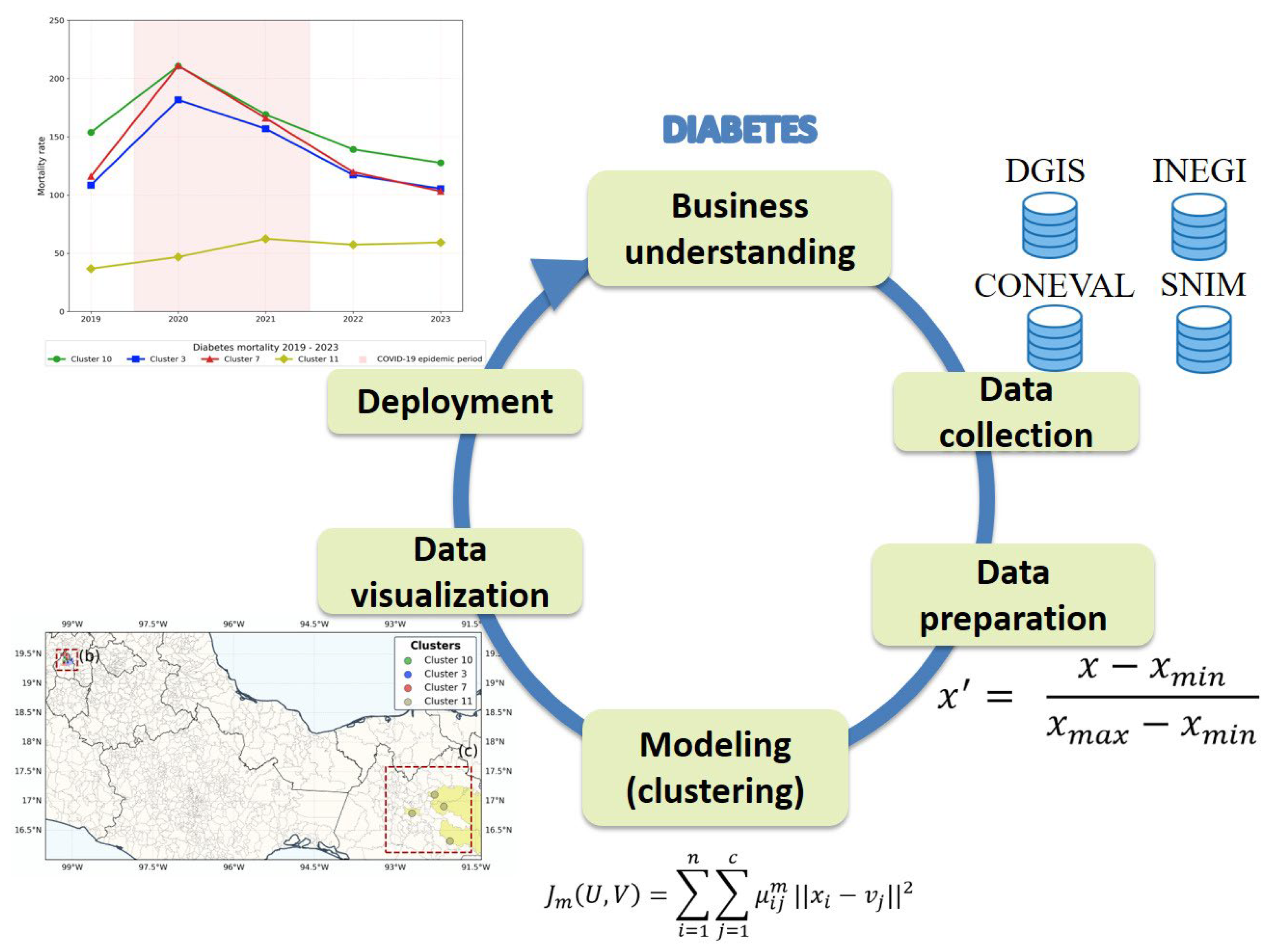
Figure 1. The Batch MFCD methodology.
Mathematics 14 00573 g001
Figure 2. The distribution of population density and poverty for municipalities of the 2020 dataset. Panel (a) shows results of clustering. Panel (b) shows clusters of interest.
Mathematics 14 00573 g002
Figure 3. The geospatial distribution of the municipalities of the clusters of interest. Panel (a) shows the distribution of clusters. Panel (b) shows the members of the CDMX clusters. Panel (c) shows the members of a cluster of Chiapas.
Mathematics 14 00573 g003
Figure 4. Trend of mortality rate of the clusters of interest.
Mathematics 14 00573 g004
Figure 5. Trend of the four main causes of death in Mexico.
Mathematics 14 00573 g005
Figure 6. Trends of mortality rates in the entire Mexico and in the 234 municipalities studied.
Mathematics 14 00573 g006
Table 1. Origin of datasets and their general characteristics.
SourceDatasetNumber of
Records
Number of
Attributes
DGIS (Dirección General de
Información en Salud) [51]
Death records 2019–20234,604,36059
INEGI (Instituto Nacional de
Estadística y Geografía) [52,53]
Population and housing census 2020195,663286
CONEVAL (Consejo Nacional de Evaluación de la Política de
Desarrollo Social) [54]
Poverty indicators 20202469145
SNIM (Sistema Nacional de
Información Municipal) [55]
Municipal information
records
24775
Table 2. Attributes selected from each dataset.
DatasetBase Attributes
Death records 2019–2023 (DGIS)State code, municipality code, death cause, and date of death
Population and housing census 2020 (INEGI)State code, state name, municipality code,
municipality name, total population, longitude, latitude, and altitude
Poverty indicators 2020 (CONEVAL)State code, municipality code, and percentage of
population in poverty
Municipal information records (SNIM)State code, state name, municipality code,
municipality name, and municipality area in km2
Table 3. Clustering results obtained with different values of c.
Index141618202224
Partition coefficient0.91550.91550.92150.93760.92840.9299
Partition entropy0.15400.15400.14810.12100.13540.1336
Silhouette index0.44810.44810.44110.46390.44760.4551
Table 4. Results for the clustering of the dataset for 2020.
ClusterPopulation
Density
Population in PovertyNumber of
Municipalities
Average Mortality Rate
100.96190.137230.5970
30.94860.434420.5101
190.73390.693610.3699
70.72370.254940.5975
170.49600.329660.4016
50.47330.645420.3876
160.40300.086630.3628
90.27340.265350.4049
40.26960.426580.3077
120.17270.3479140.3247
00.15760.082230.2110
130.10900.214790.1731
180.10350.4866160.3775
10.02360.5593330.4097
140.01680.3247260.2721
20.01730.4171250.3471
60.01610.1768310.2196
80.01610.2548200.2469
150.01670.7180190.3934
110.00560.978840.1078
Table 5. Clusters of interest.
YearClusterPopulation
Density
Population in PovertyAverage Mortality RateAverage Age at Death
2019100.96180.1371153.801968.4934
30.94850.4343108.497268.3355
70.72220.2560115.975668.8533
110.00560.978636.883363.5742
2020100.96180.1371210.807668.5474
30.94850.4343181.678367.6134
70.72220.2560210.983168.8384
110.00560.978646.904364.0137
2021100.96180.1371169.108369.0481
30.94850.4343156.938268.8953
70.72220.2560166.064269.5284
110.00560.978662.424564.3385
2022100.96180.1371139.209870.0100
30.94850.4343117.285770.3936
70.72220.2560119.814970.7411
110.00560.978657.454663.2591
2023100.96180.1371127.674170.0408
30.94850.4343105.527370.1341
70.72220.2560103.239970.6185
110.00560.978659.368063.4612
Table 6. Municipalities of the groups of interest.
ClusterStateMunicipality
10CDMXIztacalco
CDMXBenito Juárez
CDMXCuauhtémoc
3CDMXIztapalapa
Estado de MéxicoNezahualcóyotl
7CDMXAzcapotzalco
CDMXCoyoacán
CDMXGustavo A. Madero
CDMXVenustiano Carranza
11ChiapasChamula
ChiapasChilón
ChiapasLas Margaritas
ChiapasOcosingo
Disclaimer/Publisher’s Note: The statements, opinions and data contained in all publications are solely those of the individual author(s) and contributor(s) and not of MDPI and/or the editor(s). MDPI and/or the editor(s) disclaim responsibility for any injury to people or property resulting from any ideas, methods, instructions or products referred to in the content.