A New Hybrid Stochastic SIS Co-Infection Model with Two Primary Strains Under Markov Regime Switching and Lévy Jumps

Abstract

We study a hybrid stochastic SIS co-infection model for two primary strains and a co-infected class with Crowley–Martin incidence, Markovian regime switching, and Lévy jumps. The model is a four-dimensional regime-switching Lévy-driven SDE system with state-dependent diffusion and jump coefficients. Under natural integrability conditions on the jumps and a mild structural assumption on removal rates, we prove uniform high-order moment bounds for the total population, establish pathwise sublinear growth, and derive strong laws of large numbers for all Brownian and Lévy martingales, reducing the long-time analysis to deterministic time averages. Using logarithmic Lyapunov functionals for the infective classes, we introduce four noise-corrected effective growth parameters ${\lambda }_1,\dots ,{\lambda }_4$ and two interaction matrices $A,B$ that encode the combined impact of Crowley–Martin saturation, regime switching, and jump noise. In terms of explicit inequalities involving ${\lambda }_k$ and the entries of $A,B$, we obtain sharp almost-sure criteria for extinction of all infectives, persistence with competitive exclusion, and coexistence in mean of both primary strains, together with the induced long-term behaviour of the co-infected class. Numerical simulations with regime switching and compensated Poisson jumps illustrate and support these thresholds. This provides, to our knowledge, the first rigorous extinction-exclusion-coexistence theory for a multi-strain SIS co-infection model under the joint influence of Crowley–Martin incidence, Markov switching, and Lévy perturbations.

1. Introduction

Many pathogens circulate in multiple antigenic or virulence variants that coexist, compete, and sometimes synergise within the same host population [1]. Examples range from influenza and dengue serotypes to antibiotic-resistant bacterial strains and emerging viral variants [2,3]. In such settings, individuals may experience repeated infections with different strains [4], and co-infection can alter disease severity [5], transmission, and removal rates [6]. Capturing these mechanisms in a mathematically tractable way requires going beyond single-strain SIR/SIS models and incorporating both competition between primary strains and the possibility of a co-infected class [7].

Deterministic two-strain SIS models with competition have been extensively studied, typically under bilinear incidence and in the absence of co-infected hosts [8,9]. Classical results show that small differences in effective reproduction numbers can lead to competitive exclusion of the weaker strain, whereas specific non-linearities or additional structure can sustain coexistence [10,11]. When co-infection is allowed, the dynamics become richer: the co-infected class may act as a bridge for transmission or as a dead end, and the long-term behaviour depends in a delicate way on how co-infection modifies infectivity and removal [12]. However, these deterministic analyses implicitly assume a homogeneous, time-invariant environment and smooth changes in transmission, which is rarely realistic [13].

In practice, transmission of each strain is affected by several sources of randomness [14,15]. First, behavioural changes and saturation effects reduce the per-capita infection rate when either the pool of susceptibles or the number of infectives becomes large [16,17]. A natural way to represent such effects is to replace bilinear incidence by a Crowley–Martin-type term, where the force of infection saturates simultaneously in susceptibles and infectives [18]. Second, contact patterns and control measures (e.g., non-pharmaceutical interventions, changes in testing or treatment) can switch abruptly between regimes on a time scale comparable to the epidemic dynamics [19,20]. This motivates the use of Markovian regime switching to model the temporal variability of transmission rates. Third, epidemics are subject to both continuous fluctuations (background noise, demographic variability) and sudden shocks such as super-spreading events, importation bursts, or abrupt loss of immunity [21]. Mathematically, these effects are well captured by hybrid stochastic systems with multiplicative Brownian noise and Lévy jumps.

There is by now a substantial literature on stochastic epidemic models with either Brownian noise or Lévy jumps, and on regime-switching SDE models where parameters such as transmission or removal rates follow a finite-state Markov chain [22,23]. However, most existing works focus on single-strain models, often with bilinear incidence, and treat either diffusion or jump perturbations but not both [24]. The results for multi-strain competition models with co-infection are predominantly deterministic, and the few stochastic extensions usually neglect regime switching and jump noise, or impose simplified linear incidence and absence of co-infected classes. To the best of our knowledge, there is no rigorous analysis of a hybrid two-strain SIS co-infection model that simultaneously incorporates Crowley–Martin behavioural saturation, Markovian switching, and Lévy-type jump perturbations.

The aim of this paper is to fill this gap. We formulate and analyse a four-dimensional hybrid stochastic SIS model describing the interaction of two primary strains and a co-infected class. The compartments are the susceptible population S, the individuals infected only by the low-virulence strain $I_1$, those infected only by the high-virulence strain $I_2$, and the co-infected class $I_{12}$. Transmission of each primary strain occurs through a Crowley–Martin incidence term that saturates in both susceptibles and infectives, while co-infection is represented by bilinear terms coupling $I_1$ and $I_2$. The transmission rates ${\beta }_1$ and ${\beta }_2$ are modulated by a finite-state continuous-time Markov chain $J\left(t\right)$ describing random regime changes in the environment, behaviour, or control intensity. On top of this deterministic skeleton, we superimpose compartment-specific multiplicative Brownian noise and common compensated Poisson jumps, modelling respectively continuous fluctuations and rare large shocks in the epidemic dynamics.

From a mathematical viewpoint, the resulting model is a non-linear regime-switching Lévy-driven SDE system with non-globally Lipschitz drift and non-linear, state-dependent diffusion and jump coefficients. The Crowley–Martin incidence and the co-infection terms prevent the direct use of standard linear-growth conditions, while the combination of switching, diffusion, and Lévy noise complicates the long-term analysis. Our first task is therefore to establish a robust well-posedness and pathwise control theory for this hybrid system. We prove that, under natural moment and integrability assumptions on the jump amplitudes and a mild structural condition on the removal rates, the model admits a unique global positive strong solution for any non-negative initial condition. Using a polynomial Lyapunov function based on the total population $N\left(t\right)=S\left(t\right)+I_1\left(t\right)+I_2\left(t\right)+I_{12}\left(t\right)$, we show that all moments of $N\left(t\right)$ of sufficiently high order remain uniformly bounded in time, and that $N\left(t\right)/t\to 0$ almost surely. In parallel, we derive strong laws of large numbers for the Brownian and Lévy martingales generated by the model, which ensure that time-averaged stochastic integrals vanish almost surely and allow us to reduce the asymptotic analysis to deterministic averaged quantities.

On this pathwise foundation, we develop a logarithmic Lyapunov framework for the primary infective classes $I_1$ and $I_2$. By applying Itô’s formula to $\log I_i\left(t\right)$ and using the moment bounds and martingale strong laws, we obtain almost-sure upper and lower bounds on the long-time growth rates $\frac{1}{t}\log I_i\left(t\right)$. These bounds are expressed in terms of four effective growth parameters ${\lambda }_1,\dots ,{\lambda }_4$ and two $2\times 2$ matrices of interaction coefficients $A=\left(a_{ij}\right)$ and $B=\left(b_{ij}\right)$. The parameters ${\lambda }_k$ combine the regime-switching structure, the Crowley–Martin saturation, and explicit corrections induced by Brownian and Lévy noise, while the entries of A and B quantify how the presence of each strain reduces the growth of the other through behavioural saturation and removal. This leads to sharp and fully explicit criteria for extinction, competitive exclusion, and coexistence in mean of the two primary strains, and to a transparent characterisation of the long-term mean burden of the co-infected class.

The main contributions of this work can be summarised as follows:

• We formulate a hybrid four-compartment SIS co-infection model that simultaneously incorporates Crowley–Martin behavioural saturation, Markovian regime switching in transmission rates, and Lévy jump perturbations, thus providing a coherent modelling framework for two-strain competition in a randomly switching and shock-prone environment.
• We prove pathwise sublinear growth of the total population and strong laws of large numbers for the associated Brownian and Lévy martingales.
• Using logarithmic Lyapunov functionals and the balance relations of the model, we derive new noise-corrected threshold quantities ${\lambda }_1,\dots ,{\lambda }_4$ and interaction matrices $A,B$, and we express extinction, single-strain persistence with exclusion of the competitor, and coexistence in mean of both primary strains in terms of explicit inequalities involving these quantities.
• We show that the co-infected class admits a well-defined long-term mean burden determined by the time-averaged co-infection rates, thereby quantifying how the interaction between the two primary strains is reflected in the mean level of co-infection. Numerical simulations based on an Euler–Maruyama scheme with regime switching and compensated Poisson jumps illustrate the different asymptotic regimes and confirm the sharpness of the theoretical thresholds.

To our knowledge, this is the first work to obtain rigorous extinction, exclusion, and coexistence-in-mean results for a multi-strain SIS co-infection model under the combined influence of Crowley–Martin incidence, Markovian regime switching, and Lévy jumps. The methodology developed here, in particular the interplay between polynomial and logarithmic Lyapunov functions and martingale strong laws in a hybrid stochastic environment, is of independent interest and can be adapted to other multi-strain and co-infection systems with non-linear incidence and hybrid noise.

Finally, we briefly outline the organisation of the paper. In Section 2, we introduce the deterministic two-strain SIS co-infection model, the Crowley–Martin incidence structure, and its hybrid stochastic extension with regime switching, Brownian noise, and Lévy jumps. Section 3 is devoted to the well-posedness analysis and establish pathwise sublinear growth together with strong laws of large numbers for the driving martingales. In Section 4, we develop the logarithmic Lyapunov framework, introduce the effective growth parameters ${\lambda }_1,\dots ,{\lambda }_4$ and the interaction matrices $A,B$, and derive sharp criteria for extinction, competitive exclusion, and coexistence in the mean of the two primary strains, together with the induced behaviour of the co-infected class. The theoretical results are illustrated and validated by numerical experiments in Section 5, where we simulate the hybrid system under different parameter regimes and noise configurations.

2. Model Formulation

We consider a homogeneously mixing SIS-type host population exposed to two pathogens (strain 1 and strain 2) with the possibility of co-infection. At time $t\ge 0$,

• $S\left(t\right)$ denotes the density of susceptible hosts;
• $I_1\left(t\right)$ denotes the density of hosts infected by strain 1 only;
• $I_2\left(t\right)$ denotes the density of hosts infected by strain 2 only;
• $I_{12}\left(t\right)$ denotes the density of hosts simultaneously infected by both strains (co-infected hosts).

Each host belongs to exactly one of these four compartments, so that the total host density is

$$N\left(t\right):=S\left(t\right)+I_1\left(t\right)+I_2\left(t\right)+I_{12}\left(t\right).$$

2.1. Demography, Recovery, and Co-Infection Structure

New hosts are recruited (by birth or immigration) at a constant rate $\mathrm{\Lambda }>0$. All hosts are subject to natural removal at a rate of $\mu >0$. Infected and co-infected hosts may in addition experience strain-dependent disease-induced removal:

$${\delta }_1,{\delta }_2,{\delta }_{12}\ge 0,$$

acting on $I_1,I_2,I_{12}$, respectively.

Recovery from infection occurs at rates

$${\gamma }_1,{\gamma }_2,{\gamma }_{12}\ge 0,$$

and follows an SIS paradigm: recovered individuals immediately lose short-lived immunity and return to the susceptible class. Thus the flows ${\gamma }_1{I}_1$, ${\gamma }_2{I}_2$, and ${\gamma }_{12}{I}_{12}$ go directly back into S.

Co-infection occurs when a host already infected by one strain acquires the other strain. We model this by transfer rates

$${\mathrm{\Psi }}_1(I_1,I_2),{\mathrm{\Psi }}_2(I_1,I_2),$$

from $I_1$ and $I_2$ into the co-infected class $I_{12}$. A natural and widely used choice is a bilinear (mass-action) form

$${\mathrm{\Psi }}_1(I_1,I_2):={\chi }_1{I}_1{I}_2,{\mathrm{\Psi }}_2(I_1,I_2):={\chi }_2{I}_1{I}_2,$$

(1)

with ${\chi }_1,{\chi }_2\ge 0$ quantifying how easily individuals in $I_1$ acquire strain 2 and individuals in $I_2$ acquire strain 1, respectively.

2.2. Crowley–Martin Transmission with Co-Infection

Primary infection of susceptibles is described by a Crowley–Martin-type nonlinear incidence that saturates with respect to both susceptibles and infectious individuals (including co-infected hosts). Biologically, this form accounts for and behavioural responses: when the susceptible pool is large, individuals cannot increase risky contacts indefinitely (time/space constraints, awareness, protective behaviour), and when infectious prevalence is high, transmission does not grow proportionally because contacts become “redundant” (repeated contacts with already infected individuals), and mixing is effectively limited by crowding and avoidance. In particular, the saturating terms in the denominator can represent (i) reduced effective contact due to prevention and risk perception, (ii) competition among infectives for susceptible contacts, and (iii) congestion effects in high-density settings.

Let ${\beta }_1,{\beta }_2>0$ be baseline transmission rates for strains 1 and 2, and introduce:

• coefficients ${\alpha }_{11},{\alpha }_{12},{\alpha }_{21},{\alpha }_{22}>0$, which control saturation with respect to singly infected and co-infected hosts for each strain (larger $\alpha$ means stronger inhibition of transmission at high prevalence, e.g., via avoidance, isolation, or contact “wastage”);
• a common crowding parameter $\kappa >0$ describing behavioural saturation among susceptibles (larger $\kappa$ reflects stronger self-protection or reduced effective mixing when S is large).

We define the effective forces of infection as

$${\mathrm{\Phi }}_1(S,I_1,I_{12}):={\displaystyle \frac{{\beta }_{1}S(I_1+q_1{I}_{12})}{1+{\alpha }_{11}{I}_1+{\alpha }_{12}{I}_{12}+\kappa S}},{\mathrm{\Phi }}_2(S,I_2,I_{12}):={\displaystyle \frac{{\beta }_{2}S(I_2+q_2{I}_{12})}{1+{\alpha }_{21}{I}_2+{\alpha }_{22}{I}_{12}+\kappa S}},$$

(2)

where $q_1,q_2\in [0,1]$ encode the relative infectiousness of co-infected hosts compared with singly infected ones for the two strains (for instance, $q_1<1$ means co-infected hosts contribute less effectively to the transmission of strain 1 than hosts in $I_1$).

2.3. Deterministic SIS Co-Infection System

Combining demography, recovery, primary infection and co-infection, the deterministic dynamics are governed by

$$\left\{\begin{array}{cc}\hfill {\displaystyle \frac{\mathrm{d}S\left(t\right)}{\mathrm{d}t}}& =\mathrm{\Lambda }-{\mathrm{\Phi }}_1\left(S\left(t\right),I_1\left(t\right),I_{12}\left(t\right)\right)-{\mathrm{\Phi }}_2\left(S\left(t\right),I_2\left(t\right),I_{12}\left(t\right)\right)-\mu S\left(t\right)\hfill \\ \hfill & +{\gamma }_1{I}_1\left(t\right)+{\gamma }_2{I}_2\left(t\right)+{\gamma }_{12}{I}_{12}\left(t\right),\hfill \\ \hfill {\displaystyle \frac{\mathrm{d}{I}_1\left(t\right)}{\mathrm{d}t}}& ={\mathrm{\Phi }}_1\left(S\left(t\right),I_1\left(t\right),I_{12}\left(t\right)\right)-\left(\mu +{\delta }_1+{\gamma }_1\right)I_1\left(t\right)-{\mathrm{\Psi }}_1\left(I_1\left(t\right),I_2\left(t\right)\right),\hfill \\ \hfill {\displaystyle \frac{\mathrm{d}{I}_2\left(t\right)}{\mathrm{d}t}}& ={\mathrm{\Phi }}_2\left(S\left(t\right),I_2\left(t\right),I_{12}\left(t\right)\right)-\left(\mu +{\delta }_2+{\gamma }_2\right)I_2\left(t\right)-{\mathrm{\Psi }}_2\left(I_1\left(t\right),I_2\left(t\right)\right),\hfill \\ \hfill {\displaystyle \frac{\mathrm{d}{I}_{12}\left(t\right)}{\mathrm{d}t}}& ={\mathrm{\Psi }}_1\left(I_1\left(t\right),I_2\left(t\right)\right)+{\mathrm{\Psi }}_2\left(I_1\left(t\right),I_2\left(t\right)\right)-\left(\mu +{\delta }_{12}+{\gamma }_{12}\right)I_{12}\left(t\right).\hfill \end{array}\right.$$

(3)

The first equation describes the susceptible population: susceptibles arerecruited, infected by either strain via ${\mathrm{\Phi }}_1$ and ${\mathrm{\Phi }}_2$, removed naturally at rate $\mu$, and replenished by recovery from all infectious classes. The second and third equations describe single infections, with transition to the co-infected class through ${\mathrm{\Psi }}_1$ and ${\mathrm{\Psi }}_2$. The fourth equation governs the co-infected population, which receives inflow from co-infection of singly infected hosts and loses individuals through natural mortality, disease-induced removal, and recovery. The biological interpretations of all parameters are provided in

Table 1. Biological meaning of model parameters.

Parameter	Biological Meaning
$\mathrm{\Lambda }$	Constant recruitment (birth/immigration) rate of hosts into the population (into S).
$\mu$	Natural removal rate (background mortality/emigration) affecting all host classes.
${\delta }_1$	Disease-induced removal rate for hosts infected with strain 1 only ($I_1$).
${\delta }_2$	Disease-induced removal rate for hosts infected with strain 2 only ($I_2$).
${\delta }_{12}$	Disease-induced removal rate for co-infected hosts ($I_{12}$).
${\gamma }_1$	Recovery rate from strain 1 infection (from $I_1$ back to S; SIS clearance).
${\gamma }_2$	Recovery rate from strain 2 infection (from $I_2$ back to S; SIS clearance).
${\gamma }_{12}$	Recovery rate from co-infection (from $I_{12}$ back to S; SIS clearance).
${\beta }_1$	Baseline transmission rate of strain 1 in primary infection of susceptibles.
${\beta }_2$	Baseline transmission rate of strain 2 in primary infection of susceptibles.
$q_1$	Relative infectiousness of co-infected hosts for transmitting strain 1 (contribution of $I_{12}$ to strain 1 transmission).
$q_2$	Relative infectiousness of co-infected hosts for transmitting strain 2 (contribution of $I_{12}$ to strain 2 transmission).
${\alpha }_{11}$	Saturation coefficient (Crowley–Martin) associated with $I_1$ in strain 1 incidence; reduces transmission when $I_1$ is large.
${\alpha }_{12}$	Saturation coefficient associated with $I_{12}$ in strain 1 incidence; reduces strain 1 transmission when co-infection is prevalent.
${\alpha }_{21}$	Saturation coefficient associated with $I_2$ in strain 2 incidence; reduces transmission when $I_2$ is large.
${\alpha }_{22}$	Saturation coefficient associated with $I_{12}$ in strain 2 incidence; reduces strain 2 transmission when co-infection is prevalent.
$\kappa$	Susceptible-side crowding/behavioural saturation parameter in the incidence; limits effective contacts as S increases.
${\chi }_1$	Co-infection acquisition coefficient for $I_1\to I_{12}$ (rate at which strain 1 infected hosts acquire strain 2 through contact with $I_2$).
${\chi }_2$	Co-infection acquisition coefficient for $I_2\to I_{12}$ (rate at which strain 2 infected hosts acquire strain 1 through contact with $I_1$).

.

System (3) defines the deterministic skeleton of our model. It admits the disease-free equilibrium

$$(S^{★},I_1^{★},I_2^{★},I_{12}^{★})=\left({\displaystyle \frac{\mathrm{\Lambda }}{\mu }},0,0,0\right).$$

2.4. Stochastic Perturbations: Regime Switching and Lévy Jumps

To account for environmental variability, changes in contact patterns, and rare but significant shocks (superspreading events, abrupt interventions, etc.), we embed (3) in a hybrid stochastic framework.

We work on a complete filtered probability space $(\mathrm{\Omega },\mathcal{F},{\left\{{\mathcal{F}}_t\right\}}_{t\ge 0},\mathbb{P})$ satisfying the usual conditions, and introduce:

• four independent standard Brownian motions

  $$W_S,W_1,W_2,W_{12},$$

  modelling small, continuous fluctuations in the net growth of $S,I_1,I_2,I_{12}$;
• a Poisson random measure $N(\mathrm{d}t,\mathrm{d}u)$ on ${\mathbb{R}}_{+}\times \mathcal{U}$ with characteristic measure $\nu \left(\mathrm{d}u\right)$, representing random jump events of type $u\in \mathcal{U}$ (for example, mass gatherings or sudden policy shifts); its compensated version is

  $$\tilde{N}(\mathrm{d}t,\mathrm{d}u):=N(\mathrm{d}t,\mathrm{d}u)-\nu \left(\mathrm{d}u\right)\mathrm{d}t;$$
• an irreducible finite-state continuous-time Markov chain $J\left(t\right)$ with state space $\mathcal{M}:=\{1,\dots ,m\}$ and generator $Q={\left(q_{kl}\right)}_{k,l\in \mathcal{M}}$, encoding random regime switching (seasonality, changes in non-pharmaceutical interventions, behavioural phases, etc.).

We assume that $W_S,W_1,W_2,W_{12}$, N, and J are mutually independent.

The baseline transmission rates become regime-dependent:

$${\beta }_1\left(J\left(t\right)\right),{\beta }_2\left(J\left(t\right)\right)>0.$$

Accordingly, the Crowley-Martin incidence terms in (2) are replaced by

$${\mathrm{\Phi }}_1\left(S,I_1,I_{12},J\left(t\right)\right):={\displaystyle \frac{{\beta }_1\left(J\left(t\right)\right)S(I_1+q_1{I}_{12})}{1+{\alpha }_{11}{I}_1+{\alpha }_{12}{I}_{12}+\kappa S}},{\mathrm{\Phi }}_2\left(S,I_2,I_{12},J\left(t\right)\right):={\displaystyle \frac{{\beta }_2\left(J\left(t\right)\right)S(I_2+q_2{I}_{12})}{1+{\alpha }_{21}{I}_2+{\alpha }_{22}{I}_{12}+\kappa S}}.$$

(4)

We introduce nonnegative diffusion intensities

$${\sigma }_S,{\sigma }_1,{\sigma }_2,{\sigma }_{12}\ge 0$$

and jump amplitude functions

$$h_S,h_1,h_2,h_{12}:\mathcal{U}\to \mathbb{R},$$

where $h_X\left(u\right)$ represents the relative jump size experienced by compartment $X\in \{S,I_1,I_2,I_{12}\}$ during an event of type u. The multiplicative forms ${\sigma }_{X}X\left(t\right)\mathrm{d}{W}_X\left(t\right)$ and $h_X\left(u\right)X\left(t^{-}\right)$ ensure that the noise intensity scales with the current population size. We assume

$$h_X\left(u\right)>-1,u\in \mathcal{U},X\in \{S,I_1,I_2,I_{12}\},$$

so that jumps preserve positivity.

2.5. Hybrid Stochastic SIS Co-Infection Model

The resulting hybrid stochastic co-infection model is the following system of SDEs with regime switching and Lévy jumps:

$$\left\{\begin{array}{cc}\hfill \mathrm{d}S\left(t\right)& =[\mathrm{\Lambda }-{\mathrm{\Phi }}_1\left(S\left(t\right),I_1\left(t\right),I_{12}\left(t\right),J\left(t\right)\right)-{\mathrm{\Phi }}_2\left(S\left(t\right),I_2\left(t\right),I_{12}\left(t\right),J\left(t\right)\right)-\mu S\left(t\right)\hfill \\ \hfill & +{\gamma }_1{I}_1\left(t\right)+{\gamma }_2{I}_2\left(t\right)+{\gamma }_{12}{I}_{12}\left(t\right)]\mathrm{d}t+{\sigma }_{S}S\left(t\right)\mathrm{d}{W}_S\left(t\right)+{\int }_{\mathcal{U}}{h}_S\left(u\right)S\left(t^{-}\right)\tilde{N}(\mathrm{d}t,\mathrm{d}u),\hfill \\ \hfill \mathrm{d}{I}_1\left(t\right)& =\left[{\mathrm{\Phi }}_1\left(S\left(t\right),I_1\left(t\right),I_{12}\left(t\right),J\left(t\right)\right)-\left(\mu +{\delta }_1+{\gamma }_1\right)I_1\left(t\right)-{\mathrm{\Psi }}_1\left(I_1\left(t\right),I_2\left(t\right)\right)\right]\mathrm{d}t\hfill \\ \hfill & +{\sigma }_1{I}_1\left(t\right)\mathrm{d}{W}_1\left(t\right)+{\int }_{\mathcal{U}}{h}_1\left(u\right)I_1\left(t^{-}\right)\tilde{N}(\mathrm{d}t,\mathrm{d}u),\hfill \\ \hfill \mathrm{d}{I}_2\left(t\right)& =\left[{\mathrm{\Phi }}_2\left(S\left(t\right),I_2\left(t\right),I_{12}\left(t\right),J\left(t\right)\right)-\left(\mu +{\delta }_2+{\gamma }_2\right)I_2\left(t\right)-{\mathrm{\Psi }}_2\left(I_1\left(t\right),I_2\left(t\right)\right)\right]\mathrm{d}t\hfill \\ \hfill & +{\sigma }_2{I}_2\left(t\right)\mathrm{d}{W}_2\left(t\right)+{\int }_{\mathcal{U}}{h}_2\left(u\right)I_2\left(t^{-}\right)\tilde{N}(\mathrm{d}t,\mathrm{d}u),\hfill \\ \hfill \mathrm{d}{I}_{12}\left(t\right)& =\left[{\mathrm{\Psi }}_1\left(I_1\left(t\right),I_2\left(t\right)\right)+{\mathrm{\Psi }}_2\left(I_1\left(t\right),I_2\left(t\right)\right)-\left(\mu +{\delta }_{12}+{\gamma }_{12}\right)I_{12}\left(t\right)\right]\mathrm{d}t\hfill \\ \hfill & +{\sigma }_{12}{I}_{12}\left(t\right)\mathrm{d}{W}_{12}\left(t\right)+{\int }_{\mathcal{U}}{h}_{12}\left(u\right)I_{12}\left(t^{-}\right)\tilde{N}(\mathrm{d}t,\mathrm{d}u).\hfill \end{array}\right.$$

(5)

The drift part of (5) coincides with the deterministic co-infection system (3), while the diffusion and jump terms encode continuous environmental noise and rare abrupt shocks. Regime switching enters through the transmission rates ${\beta }_1\left(J\left(t\right)\right),{\beta }_2\left(J\left(t\right)\right)$ in the Crowley–Martin incidence (4). This four-dimensional hybrid system provides a tractable yet flexible framework to analyse extinction, persistence, and coexistence of the two strains and the co-infected class under complex random perturbations.

3. Well-Posedness and Asymptotic Pathwise Estimates

Throughout, we work on a stochastic basis and with the driving processes introduced in Section 2, and we assume that

$$\left(S\left(0\right),I_1\left(0\right),I_2\left(0\right),I_{12}\left(0\right)\right)\in {\mathbb{R}}_{+}^4,J\left(0\right)\in \mathcal{M}.$$

3.1. Assumptions and Global Positivity

We first collect the structural conditions on the jump coefficients and on the demographic parameters.

Assumption 1.

For each compartment $X\in \{S,I_1,I_2,I_{12}\}$, the jump amplitude function $h_X:\mathcal{U}\to \mathbb{R}$ satisfies:

(H1) 

${\displaystyle {\int }_{\mathcal{U}}{h}_X{\left(u\right)}^2\nu \left(\mathrm{d}u\right)<\infty }$.

(H2) 

${\displaystyle {\int }_{\mathcal{U}}\left|h_X\left(u\right)-\log \left(1+h_X\left(u\right)\right)\right|\nu \left(\mathrm{d}u\right)<\infty }$.

In addition, we assume

$$h_X\left(u\right)>-1,u\in \mathcal{U},X\in \{S,I_1,I_2,I_{12}\},$$

so that jumps preserve nonnegativity of each component.

Assumption 2.

The demographic parameters satisfy $\mathrm{\Lambda }>0$ and $\mu >0$. We set

$${\mu }_{*}:=\mu .$$

Let

$$N\left(t\right):=S\left(t\right)+I_1\left(t\right)+I_2\left(t\right)+I_{12}\left(t\right),{\mathbb{R}}_{+}^4:={[0,\infty )}^4,$$

and

$$W\left(t\right):={\left(W_S\left(t\right),W_1\left(t\right),W_2\left(t\right),W_{12}\left(t\right)\right)}^{\top }.$$

For later use, we rewrite system (5) in vector form. For $U={(S,I_1,I_2,I_{12})}^{\top }$ and $k\in \mathcal{M}$, define

$$\begin{array}{cc}\hfill b(U,k)& :=\left(\begin{array}{c}\mathrm{\Lambda }-{\mathrm{\Phi }}_1\left(S,I_1,I_{12},k\right)-{\mathrm{\Phi }}_2\left(S,I_2,I_{12},k\right)-\mu S+{\gamma }_1{I}_1+{\gamma }_2{I}_2+{\gamma }_{12}{I}_{12}\\ {\mathrm{\Phi }}_1\left(S,I_1,I_{12},k\right)-\left(\mu +{\delta }_1+{\gamma }_1\right)I_1-{\mathrm{\Psi }}_1(I_1,I_2)\\ {\mathrm{\Phi }}_2\left(S,I_2,I_{12},k\right)-\left(\mu +{\delta }_2+{\gamma }_2\right)I_2-{\mathrm{\Psi }}_2(I_1,I_2)\\ {\mathrm{\Psi }}_1(I_1,I_2)+{\mathrm{\Psi }}_2(I_1,I_2)-\left(\mu +{\delta }_{12}+{\gamma }_{12}\right)I_{12}\end{array}\right),\hfill \\ \hfill \Sigma \left(U\right)& :=\left(\begin{array}{cccc}{\sigma }_{S}S& 0& 0& 0\\ 0& {\sigma }_1{I}_1& 0& 0\\ 0& 0& {\sigma }_2{I}_2& 0\\ 0& 0& 0& {\sigma }_{12}{I}_{12}\end{array}\right),\hfill \\ \hfill H(U,u)& :=\left(\begin{array}{c}{h}_S\left(u\right)S\\ h_1\left(u\right)I_1\\ h_2\left(u\right)I_2\\ h_{12}\left(u\right)I_{12}\end{array}\right),u\in \mathcal{U},\hfill \end{array}$$

where ${\mathrm{\Phi }}_1$ and ${\mathrm{\Phi }}_2$ are given by (4) and ${\mathrm{\Psi }}_1,{\mathrm{\Psi }}_2$ by (1). Then, system (5) can be written compactly as

$$\mathrm{d}U\left(t\right)=b\left(U\left(t\right),J\left(t\right)\right)\mathrm{d}t+\Sigma \left(U\left(t\right)\right)\mathrm{d}W\left(t\right)+{\int }_{\mathcal{U}}H\left(U\left(t^{-}\right),u\right)\tilde{N}(\mathrm{d}t,\mathrm{d}u).$$

Lemma 1.

Suppose that Assumptions 1 and 2 hold and that the structural assumptions on the driving processes in Section 2 are satisfied. Then, for every initial condition

$$\left(S\left(0\right),I_1\left(0\right),I_2\left(0\right),I_{12}\left(0\right)\right)\in {\mathbb{R}}_{+}^4,J\left(0\right)\in \mathcal{M},$$

system (5) admits a unique global strong solution ${\left\{(S\left(t\right),I_1\left(t\right),I_2\left(t\right),I_{12}\left(t\right),J\left(t\right))\right\}}_{t\ge 0}$ such that

$$\left(S\left(t\right),I_1\left(t\right),I_2\left(t\right),I_{12}\left(t\right)\right)\in {\mathbb{R}}_{+}^4,\forall t\ge 0a.s.$$

A detailed proof of this result is provided in [23].

3.2. Higher-Order Moment Estimates and Drift-Noise Balance

We now derive a uniform higher-order moment bound for the total population. Recall that

$$N\left(t\right):=S\left(t\right)+I_1\left(t\right)+I_2\left(t\right)+I_{12}\left(t\right),t\ge 0.$$

Define the combined jump amplitude

$$G(t,u):=h_S\left(u\right)S\left(t\right)+h_1\left(u\right)I_1\left(t\right)+h_2\left(u\right)I_2\left(t\right)+h_{12}\left(u\right)I_{12}\left(t\right),t\ge 0,u\in \mathcal{U},$$

and the pointwise maximal amplitude

$$\widehat{h}\left(u\right):=\max \left\{|h_S\left(u\right)|,|h_1\left(u\right)|,|h_2\left(u\right)|,|h_{12}\left(u\right)|\right\},u\in \mathcal{U}.$$

Then, for all $t\ge 0$ and $u\in \mathcal{U}$,

$$\left|G(t,u)\right|\le |h_S\left(u\right)|S\left(t\right)+|h_1\left(u\right)|I_1\left(t\right)+|h_2\left(u\right)|I_2\left(t\right)+\left|h_{12}\left(u\right)\right|I_{12}\left(t\right)\le 4\widehat{h}\left(u\right)N\left(t\right).$$

Fix an integer $r\ge 2$ and consider the Lyapunov function

$$V\left(x\right):={(1+x)}^r,x\ge 0.$$

Assumption 3.

Let $r\ge 2$ be fixed.

(H^(r)₃)

Set

$${\sigma }^2:={\sigma }_S^2+{\sigma }_1^2+{\sigma }_2^2+{\sigma }_{12}^2,$$

and define

$$\xi \left(r\right):=C_r{\int }_{\mathcal{U}}\widehat{h}{\left(u\right)}^2\nu \left(\mathrm{d}u\right)+C_r{\int }_{\mathcal{U}}\widehat{h}{\left(u\right)}^r\nu \left(\mathrm{d}u\right),$$

where $C_r>0$ depends only on r. Assume that

$$\rho :={\mu }_{*}-{\displaystyle \frac{r-1}{2}}{\sigma }^2-{\displaystyle \frac{\xi \left(r\right)}{r}}>0.$$

(H^(r)₄)

The Lévy measure satisfies

$${\int }_{\mathcal{U}}\left|{(1+\widehat{h}\left(u\right))}^r-1\right|\nu \left(\mathrm{d}u\right)<\infty .$$

Lemma 2

(Uniform r-moment bound for $N\left(t\right)$). Suppose that Assumptions 1, 2 and 3 hold for some integer $r\ge 2$. Then, there exists a constant $K_r>0$ such that

$$\underset{t\ge 0}{\sup }\mathbb{E}\left[{(1+N\left(t\right))}^r\right]\le K_r.$$

In particular, ${\sup }_{t\ge 0}\mathbb{E}\left[N{\left(t\right)}^r\right]<\infty$.

Proof. 

First, recall the dynamics of $N\left(t\right)$. Summing the four equations in (5) and using the cancellation of the infection and co-infection terms ${\mathrm{\Phi }}_1,{\mathrm{\Phi }}_2,{\mathrm{\Psi }}_1,{\mathrm{\Psi }}_2$, we obtain

$$\mathrm{d}N\left(t\right)=b_N\left(t\right)\mathrm{d}t+\sum _{X\in \{S,I_1,I_2,I_{12}\}}{\sigma }_{X}X\left(t\right)\mathrm{d}{W}_X\left(t\right)+{\int }_{\mathcal{U}}G(t^{-},u)\tilde{N}(\mathrm{d}t,\mathrm{d}u),$$

where

$$b_N\left(t\right)=\mathrm{\Lambda }-\mu N\left(t\right)-{\delta }_1{I}_1\left(t\right)-{\delta }_2{I}_2\left(t\right)-{\delta }_{12}{I}_{12}\left(t\right)\le \mathrm{\Lambda }-{\mu }_{*}N\left(t\right),$$

by Assumption 2 (here ${\mu }_{*}=\mu >0$).

For $R\ge 1$, set ${\tau }_R:=\inf \{t\ge 0:N\left(t\right)\ge R\}$ and $N_R\left(t\right):=N(t\wedge {\tau }_R)$. Since ${\tau }_R\uparrow \infty$ almost surely, it suffices to obtain bounds that are uniform in R.

Applying Itô’s formula with jumps to $V\left(N_R\left(t\right)\right)={(1+N_R\left(t\right))}^r$ and writing $N=N_R\left(t\right)$, $G_R(t,u):=G(t,u){\mathbf{1}}_{\{t\le {\tau }_R\}}$, we obtain

$$\mathrm{d}V\left(N\right)=\mathcal{L}V\left(N\right)\mathrm{d}t+\mathrm{d}{M}_V^R\left(t\right),$$

where $M_V^R$ is a local martingale and

$$\begin{array}{cc}\hfill \mathcal{L}V\left(N\right)& =V^{\prime }\left(N\right)b_N\left(t\right)+{\displaystyle \frac{1}{2}}{V}^{″}\left(N\right){\displaystyle \frac{\mathrm{d}}{\mathrm{d}t}}{\langle N^c\rangle }_t\hfill \\ \hfill & +{\int }_{\mathcal{U}}\left[V\left(N+G_R(t,u)\right)-V\left(N\right)-V^{\prime }\left(N\right)G_R(t,u)\right]\nu \left(\mathrm{d}u\right),\hfill \end{array}$$

with $V^{\prime }\left(x\right)=r{(1+x)}^{r-1}$, $V^{″}\left(x\right)=r(r-1){(1+x)}^{r-2}$, and

$${\displaystyle \frac{\mathrm{d}}{\mathrm{d}t}}{\langle N^c\rangle }_t=\sum _{X\in \{S,I_1,I_2,I_{12}\}}{\sigma }_X^{2}X{\left(t\right)}^2\le {\sigma }^{2}N{\left(t\right)}^2\le {\sigma }^2{N}_R{\left(t\right)}^2={\sigma }^2{N}^2.$$

Using $b_N\left(t\right)\le \mathrm{\Lambda }-{\mu }_{*}N$, we obtain

$$\begin{array}{cc}\hfill \mathcal{L}V\left(N\right)& \le r{(1+N)}^{r-1}(\mathrm{\Lambda }-{\mu }_{*}N)+{\displaystyle \frac{1}{2}}r(r-1){\sigma }^2{(1+N)}^{r-2}{N}^2\hfill \\ \hfill & +{\int }_{\mathcal{U}}\left[{(1+N+G_R)}^r-{(1+N)}^r-r{(1+N)}^{r-1}{G}_R\right]\nu \left(\mathrm{d}u\right).\hfill \end{array}$$

For fixed $N\ge 0$ and $u\in \mathcal{U}$, Taylor’s theorem with integral remainder gives, for some $\theta =\theta (N,G_R)\in (0,1)$,

$${(1+N+G_R)}^r-{(1+N)}^r-r{(1+N)}^{r-1}{G}_R={\displaystyle \frac{r(r-1)}{2}}{\left(1+N+\theta G_R\right)}^{r-2}{G}_R^2.$$

We first check that the factor ${\left(1+N+\theta G_R\right)}^{r-2}$ is well defined and nonnegative. For each $u\in \mathcal{U}$ set

$$m\left(u\right):=\min \left\{h_S\left(u\right),h_1\left(u\right),h_2\left(u\right),h_{12}\left(u\right)\right\}.$$

By Assumption 1 we have $h_X\left(u\right)>-1$ for all compartments $X\in \{S,I_1,I_2,I_{12}\}$ and all $u\in \mathcal{U}$, hence $m\left(u\right)>-1$. Since $S,I_1,I_2,I_{12}\ge 0$, it follows that

$$G_R(t,u)=G(t,u){\mathbf{1}}_{\{t\le {\tau }_R\}}\ge m\left(u\right)N\left(t\right){\mathbf{1}}_{\{t\le {\tau }_R\}}.$$

Thus, for $t\le {\tau }_R$,

$$1+N+\theta G_R\ge 1+N\left(1+\theta m\left(u\right)\right).$$

Because $m\left(u\right)>-1$ and $\theta \in (0,1)$, we have $1+\theta m\left(u\right)>0$, so $1+N+\theta G_R>0$. Hence ${\left(1+N+\theta G_R\right)}^{r-2}$ is well defined and nonnegative.

On the other hand, using $|G_R| \le 4\widehat{h}\left(u\right)N$,

$$1+N+\theta G_R\le 1+N+\left|G_R\right|\le 1+N+4\widehat{h}\left(u\right)N\le (1+N)\left(1+4\widehat{h}\left(u\right)\right),$$

since $N\ge 0$ and $\widehat{h}\left(u\right)\ge 0$. For $r\ge 2$ and $a,b\ge 0$ we use the standard inequality ${(a+b)}^{r-2}\le 2^{r-3}(a^{r-2}+b^{r-2})$ to find

$${\left(1+4\widehat{h}\left(u\right)\right)}^{r-2}\le C_r\left(1+\widehat{h}{\left(u\right)}^{r-2}\right),$$

for some $C_r>0$ depending only on r. Absorbing numerical constants into $C_r$ and using again $|G_R|\le 4\widehat{h}\left(u\right)N$, we obtain

$${\left(1+N+\theta G_R\right)}^{r-2}{G}_R^2\le C_r{(1+N)}^{r-2}{N}^2\left(\widehat{h}{\left(u\right)}^2+\widehat{h}{\left(u\right)}^r\right).$$

Integrating over $\mathcal{U}$ and using the definition of $\xi \left(r\right)$ gives

$${\int }_{\mathcal{U}}\left[{(1+N+G_R)}^r-{(1+N)}^r-r{(1+N)}^{r-1}{G}_R\right]\nu \left(\mathrm{d}u\right)\le {(1+N)}^{r-2}{N}^2\xi \left(r\right).$$

Collecting all terms, we get

$$\begin{array}{cc}\hfill \mathcal{L}V\left(N\right)& \le r{(1+N)}^{r-1}(\mathrm{\Lambda }-{\mu }_{*}N)+{\displaystyle \frac{1}{2}}r(r-1){\sigma }^2{(1+N)}^{r-2}{N}^2+{(1+N)}^{r-2}{N}^2\xi \left(r\right)\hfill \\ \hfill & = r{(1 + N)}^{r-2}\left[(\mathrm{\Lambda }-{\mu }_{*}N)(1+N)+{\displaystyle \frac{r-1}{2}}{\sigma }^2{N}^2+{\displaystyle \frac{\xi \left(r\right)}{r}}{N}^2\right].\hfill \end{array}$$

Since

$$(\mathrm{\Lambda }-{\mu }_{*}N)(1+N)=-{\mu }_{*}{N}^2+(\mathrm{\Lambda }-{\mu }_{*})N+\mathrm{\Lambda },$$

we can rewrite this as

$$\mathcal{L}V\left(N\right)\le r{(1+N)}^{r-2}\left[-\rho N^2+(\mathrm{\Lambda }-{\mu }_{*})N+\mathrm{\Lambda }\right],$$

where

$$\rho ={\mu }_{*}-{\displaystyle \frac{r-1}{2}}{\sigma }^2-{\displaystyle \frac{\xi \left(r\right)}{r}}>0$$

by ($H_3^{\left(r\right)}$). There exists a constant $C_1>0$ such that $(\mathrm{\Lambda }-{\mu }_{*})N+\mathrm{\Lambda }\le C_1(1+N)$ for all $N\ge 0$, hence

$$\mathcal{L}V\left(N\right)\le r{(1+N)}^{r-2}\left(-\rho N^2+C_1(1+N)\right).$$

Since the negative term $-\rho N^2$ dominates for large N, we can find constants $C_2,C_3>0$, independent of R, such that

$$\mathcal{L}V\left(N\right)\le C_2-C_3{(1+N)}^r,N\ge 0.$$

(6)

Integrating the Itô decomposition for $V\left(N_R\left(t\right)\right)$ over $[0,t]$, taking expectations, and using $\mathbb{E}\left[M_V^R\left(t\right)\right]=0$, we obtain

$$\mathbb{E}\left[V\left(N_R\left(t\right)\right)\right]=V\left(N\left(0\right)\right)+\mathbb{E}{\int }_0^t\mathcal{L}V\left(N_R\left(s\right)\right)\mathrm{d}s.$$

Using (6),

$$\mathbb{E}\left[V\left(N_R\left(t\right)\right)\right]\le V\left(N\left(0\right)\right)+C_{2}t-C_3{\int }_0^t\mathbb{E}\left[V\left(N_R\left(s\right)\right)\right]\mathrm{d}s.$$

Let $u_R\left(t\right):=\mathbb{E}\left[V\left(N_R\left(t\right)\right)\right]$. Then

$$u_R\left(t\right)\le u_R\left(0\right)+C_{2}t-C_3{\int }_0^t{u}_R\left(s\right)\mathrm{d}s,t\ge 0.$$

Comparison with the solution of the linear ODE $v^{\prime }\left(t\right)=-C_{3}v\left(t\right)+C_2$, $v\left(0\right)=u_R\left(0\right)$, yields

$$u_R\left(t\right)\le u_R\left(0\right){\mathrm{e}}^{-C_{3}t}+{\displaystyle \frac{C_2}{C_3}}\left(1-{\mathrm{e}}^{-C_{3}t}\right)\le \max \left\{u_R\left(0\right),{\displaystyle \frac{C_2}{C_3}}\right\},t\ge 0.$$

Since $u_R\left(0\right)=V\left(N\left(0\right)\right)$ and the bound is uniform in R, letting $R\to \infty$ and applying Fatou’s lemma gives

$$\underset{t\ge 0}{\sup }\mathbb{E}\left[V\left(N\right(t\left)\right)\right]=\underset{t\ge 0}{\sup }\mathbb{E}\left[{(1+N\left(t\right))}^r\right]\le K_r$$

for some finite constant $K_r>0$, as claimed. □

3.3. Sublinear Pathwise Growth of the Solution

We next show that each component grows at most sublinearly in time.

Theorem 1.

Suppose that Assumptions 1–3 hold for some integer $r>2$. Then

$$\underset{t\to \infty }{\lim }{\displaystyle \frac{N\left(t\right)}{t}}=0,\mathit{almost}\mathit{surely}.$$

In particular,

$$\underset{t\to \infty }{\lim }{\displaystyle \frac{S\left(t\right)}{t}}=\underset{t\to \infty }{\lim }{\displaystyle \frac{I_1\left(t\right)}{t}}=\underset{t\to \infty }{\lim }{\displaystyle \frac{I_2\left(t\right)}{t}}=\underset{t\to \infty }{\lim }{\displaystyle \frac{I_{12}\left(t\right)}{t}}=0,\mathit{almost}\mathit{surely}.$$

Proof. 

We split the argument into three steps.

• Step 1. Control of the running r-moment of N. Let $r>2$ be as in Lemma 2. For $R\ge 1$, set

$${\tau }_R:=\inf \{t\ge 0:N\left(t\right)\ge R\},N_R\left(t\right):=N(t\wedge {\tau }_R).$$

By Lemma 1, ${\tau }_R\uparrow \infty$ almost surely as $R\to \infty$.

Let $f\left(x\right):=x^r$ for $x\ge 0$; then $f^{\prime }\left(x\right)=r{x}^{r-1}$, $f^{″}\left(x\right)=r(r-1)x^{r-2}$. Applying Itô’s formula with jumps to $f\left(N_R\left(t\right)\right)=N_R{\left(t\right)}^r$ on $[0,T]$ yields

$$N_R{\left(t\right)}^r=N_R{\left(0\right)}^r+{\int }_0^t{\mathcal{A}}_r\left(N_R\left(s\right)\right)\mathrm{d}s+M_R\left(t\right),0\le t\le T,$$

where $M_R=M_R^c+M_R^J$ is a local martingale with continuous part

$$M_R^c\left(t\right)={\int }_0^t{f}^{\prime }\left(N_R\left(s\right)\right)\sum _{X\in \{S,I_1,I_2,I_{12}\}}{\sigma }_{X}X\left(s\right)\mathrm{d}{W}_X\left(s\right),$$

and purely discontinuous part

$$M_R^J\left(t\right)={\int }_0^t{\int }_{\mathcal{U}}\left[f\left(N_R\left(s^{-}\right)+G_R(s,u)\right)-f\left(N_R\left(s^{-}\right)\right)-f^{\prime }\left(N_R\left(s^{-}\right)\right)G_R(s,u)\right]\tilde{N}(\mathrm{d}s,\mathrm{d}u),$$

with $G_R(s,u):=G(s,u){\mathbf{1}}_{\{s\le {\tau }_R\}}$. The drift term has the form

$${\mathcal{A}}_r\left(N_R\left(s\right)\right)={\mathrm{I}}_1\left(s\right)+{\mathrm{I}}_2\left(s\right)+{\mathrm{I}}_3\left(s\right),$$

where

$$\begin{array}{cc}\hfill {\mathrm{I}}_1\left(s\right)& =f^{\prime }\left(N_R\left(s\right)\right)b_N\left(s\right)=r{N}_R{\left(s\right)}^{r-1}{b}_N\left(s\right),\hfill \\ \hfill {\mathrm{I}}_2\left(s\right)& ={\displaystyle \frac{1}{2}}{f}^{″}\left(N_R\left(s\right)\right){\displaystyle \frac{\mathrm{d}}{\mathrm{d}s}}{〈N_R^c〉}_s={\displaystyle \frac{1}{2}}r(r-1)N_R{\left(s\right)}^{r-2}\sum _{X\in \{S,I_1,I_2,I_{12}\}}{\sigma }_X^{2}X{\left(s\right)}^2,\hfill \\ \hfill {\mathrm{I}}_3\left(s\right)& ={\int }_{\mathcal{U}}\left[f\left(N_R\left(s\right)+G_R(s,u)\right)-f\left(N_R\left(s\right)\right)-f^{\prime }\left(N_R\left(s\right)\right)G_R(s,u)\right]\nu \left(\mathrm{d}u\right).\hfill \end{array}$$

We now bound ${\mathcal{A}}_r$ from above in terms of $1+N_R^r$. Using $b_N\left(s\right)\le \mathrm{\Lambda }-{\mu }_{*}N\left(s\right)$ and $N_R\left(s\right)\le N\left(s\right)$, we obtain

$$|{\mathrm{I}}_1\left(s\right)|\le r{N}_R{\left(s\right)}^{r-1}\left|\mathrm{\Lambda }-{\mu }_{*}N\left(s\right)\right|\le C_1\left(N_R{\left(s\right)}^{r-1}+N_R{\left(s\right)}^r\right)\le C_1\left(1+N_R{\left(s\right)}^r\right)$$

for some constant $C_1>0$.

For the diffusion contribution, Assumption 3 gives

$$\sum _{X\in \{S,I_1,I_2,I_{12}\}}{\sigma }_X^{2}X{\left(s\right)}^2\le {\sigma }^{2}N{\left(s\right)}^2\le {\sigma }^2{N}_R{\left(s\right)}^2,$$

so

$$|{\mathrm{I}}_2\left(s\right)|\le {\displaystyle \frac{1}{2}}r(r-1){\sigma }^2{N}_R{\left(s\right)}^r\le C_2\left(1+N_R{\left(s\right)}^r\right)$$

for some constant $C_2>0$.

For the jump term, we use Taylor’s formula with integral remainder: for any $x,z\ge 0$,

$$f(x+z)-f\left(x\right)-f^{\prime }\left(x\right)z={\displaystyle \frac{r(r-1)}{2}}{\left(x+\theta z\right)}^{r-2}{z}^2$$

for some $\theta =\theta (x,z)\in (0,1)$. With $x=N_R\left(s\right)$, $z=G_R(s,u)$ this yields

$$\left|f(N_R+G_R)-f\left(N_R\right)-f^{\prime }\left(N_R\right)G_R\right|\le C_r{\left(N_R\left(s\right)+\left|G_R(s,u)\right|\right)}^{r-2}{G}_R{(s,u)}^2,$$

for a constant $C_r>0$ depending only on r.

Since $|G_R(s,u)|\le 4\widehat{h}\left(u\right)N_R\left(s\right)$ (see the definition of $\widehat{h}$), we have

$${\left(N_R+\left|G_R\right|\right)}^{r-2}{G}_R^2\le C_r{N}_R{\left(s\right)}^r\left(\widehat{h}{\left(u\right)}^2+\widehat{h}{\left(u\right)}^r\right),$$

after absorbing numerical constants into $C_r$ and using ${(a+b)}^{r-2}\le C_r(a^{r-2}+b^{r-2})$ for $a,b\ge 0$. Integrating over $\mathcal{U}$ and using the definition of $\xi \left(r\right)$ in Assumption 3, we obtain

$$|{\mathrm{I}}_3\left(s\right)|\le C_3\left(1+N_R{\left(s\right)}^r\right)$$

for some $C_3>0$. Collecting these bounds, there exists $C_4>0$, independent of R, such that

$$\left|{\mathcal{A}}_r\left(N_R\left(s\right)\right)\right|\le C_4\left(1+N_R{\left(s\right)}^r\right),s\ge 0.$$

(7)

The continuous martingale part satisfies

$${\displaystyle \frac{\mathrm{d}}{\mathrm{d}s}}{〈M_R^c〉}_s=f^{\prime }{\left(N_R\left(s\right)\right)}^2\sum _{X\in \{S,I_1,I_2,I_{12}\}}{\sigma }_X^{2}X{\left(s\right)}^2\le C_5{N}_R{\left(s\right)}^{2r},$$

for some $C_5>0$. Moreover, by the bound above on the jump increment and Assumption 3, the predictable quadratic variation of $M_R^J$ is also bounded by

$${\displaystyle \frac{\mathrm{d}}{\mathrm{d}s}}{〈M_R^J〉}_s\le C_6\left(1+N_R{\left(s\right)}^{2r}\right)$$

for a constant $C_6>0$. Applying the Burkholder–Davis–Gundy inequality to $M_R^c$ and Kunita’s inequality to $M_R^J$ (see, e.g., standard references on jump SDEs), we obtain, for some $C_7>0$ independent of R and T,

$$\mathbb{E}\left[\underset{0\le s\le T}{\sup }{\left|M_R\left(s\right)\right|}^r\right]\le C_7\mathbb{E}\left[{\left({\int }_0^T\left(1+N_R{\left(s\right)}^{2r}\right)\mathrm{d}s\right)}^{r/2}\right].$$

Using the decomposition of $N_R^r$, the bound (7), Hölder and Young inequalities, and the elementary estimate ${(1+z^{2r})}^{r/2}\le C(1+z^r)$, we infer that

$$\mathbb{E}\left[\underset{0\le s\le T}{\sup }{N}_R{\left(s\right)}^r\right]\le C_8\left(\mathbb{E}\left[N{\left(0\right)}^r\right]+\mathbb{E}{\int }_0^T\left(1+N_R{\left(s\right)}^r\right)\mathrm{d}s\right),$$

for some constant $C_8>0$ independent of R and T.

Since $N_R\left(s\right)\le N\left(s\right)$ and Lemma 2 gives ${\sup }_{s\ge 0}\mathbb{E}\left[N{\left(s\right)}^r\right]\le K_r$, we have

$$\mathbb{E}{\int }_0^T{N}_R{\left(s\right)}^r\mathrm{d}s\le {\int }_0^T\mathbb{E}\left[N{\left(s\right)}^r\right]\mathrm{d}s\le K_{r}T.$$

Hence there exists $C_9>0$, independent of R and T, such that

$$\mathbb{E}\left[\underset{0\le s\le T}{\sup }{N}_R{\left(s\right)}^r\right]\le C_9\left(1+T\right),T>0.$$

Letting $R\to \infty$ and using Fatou’s lemma yields

$$\mathbb{E}\left[\underset{0\le s\le T}{\sup }N{\left(s\right)}^r\right]\le C_9(1+T),T>0.$$

(8)

Step 2. A Borel–Cantelli argument. Fix $\epsilon >0$ and, for $n\ge 1$, define the events

$$A_n:=\left\{\underset{n\le s\le n+1}{\sup }N\left(s\right)\ge \epsilon n\right\}.$$

By Markov’s inequality and (8) with $T=n+1$,

$$\mathbb{P}\left(A_n\right)\le {\displaystyle \frac{\mathbb{E}\left[{\sup }_{n\le s\le n+1}N{\left(s\right)}^r\right]}{{\left(\epsilon n\right)}^r}}\le {\displaystyle \frac{\mathbb{E}\left[{\sup }_{0\le s\le n+1}N{\left(s\right)}^r\right]}{{\left(\epsilon n\right)}^r}}\le {\displaystyle \frac{C_9(1+n+1)}{{\epsilon }^r{n}^r}}\le {\displaystyle \frac{C_{10}}{{\epsilon }^r{n}^{r-1}}},$$

for some constant $C_{10}>0$. Since $r>2$, we have ${\sum }_{n=1}^{\infty }{n}^{-(r-1)}<\infty$, and therefore

$$\sum _{n=1}^{\infty }\mathbb{P}\left(A_n\right)<\infty .$$

By the Borel–Cantelli lemma,

$$\mathbb{P}\left(A_n\mathrm{i}.\mathrm{o}.\right)=0,$$

so there exists a random integer $n_0\left(\omega \right)$ such that, for all $n\ge n_0\left(\omega \right)$,

$$\underset{n\le s\le n+1}{\sup }N(s,\omega )<\epsilon n.$$

Step 3. Conclusion. Let $\omega$ lie in this full-probability set, and take $t\ge n_0\left(\omega \right)+1$. Set $n:=\lfloor t\rfloor$; then $n\ge n_0\left(\omega \right)$ and $t\in [n,n+1]$, so

$$N(t,\omega )\le \underset{n\le s\le n+1}{\sup }N(s,\omega )<\epsilon n\le \epsilon t.$$

Hence ${\lim \sup }_{t\to \infty }N(t,\omega )/t\le \epsilon$. Since $\epsilon >0$ was arbitrary, we conclude that

$$\underset{t\to \infty }{\lim }{\displaystyle \frac{N\left(t\right)}{t}}=0\mathrm{almost}\mathrm{surely}.$$

Finally, for all $t\ge 0$,

$$0\le S\left(t\right),I_1\left(t\right),I_2\left(t\right),I_{12}\left(t\right)\le N\left(t\right),$$

so each component satisfies the same limit, which completes the proof. □

3.4. Asymptotic Behaviour of Jump and Diffusion Martingales

We conclude this section with strong laws for the stochastic integrals driven by the Lévy jumps and the Brownian motions. These estimates will be used to average logarithmic Lyapunov functionals over large time horizons.

Theorem 2.

Under the assumptions of Theorem 1, we have, for each compartment $X\in \{S,I_1,I_2,I_{12}\}$,

$$\underset{t\to \infty }{\lim }{\displaystyle \frac{1}{t}}{\int }_0^t{\int }_{\mathcal{U}}{h}_X\left(u\right)X\left(s^{-}\right)\tilde{N}(\mathrm{d}s,\mathrm{d}u)=0,\mathit{almost}\mathit{surely}.$$

Proof. 

Fix $X\in \{S,I_1,I_2,I_{12}\}$ and set

$$J_X\left(t\right):={\int }_0^t{\int }_{\mathcal{U}}{h}_X\left(u\right)X\left(s^{-}\right)\tilde{N}(\mathrm{d}s,\mathrm{d}u),t\ge 0.$$

Then, $J_X$ is a purely discontinuous local martingale with jumps

$$\Delta J_X\left(s\right)={\int }_{\mathcal{U}}{h}_X\left(u\right)X\left(s^{-}\right)N(\left\{s\right\},\mathrm{d}u).$$

Let $r>2$ be as in Theorem 1. By the integrability assumptions on $h_X$ (which follow from Assumption 1 and the definition of $\widehat{h}$), Kunita’s inequality for pure-jump martingales gives, for all $T\ge 0$,

$$\begin{array}{cc}\hfill \mathbb{E}\left[|J_X{\left(T\right)|}^r\right]& \le C_r\mathbb{E}\left[{\left({\int }_0^T{\int }_{\mathcal{U}}{\left|h_X\left(u\right)X\left(s^{-}\right)\right|}^2\nu \left(\mathrm{d}u\right)\mathrm{d}s\right)}^{r/2}\right]\hfill \\ \hfill & +C_r\mathbb{E}\left[{\int }_0^T{\int }_{\mathcal{U}}{\left|h_X\left(u\right)X\left(s^{-}\right)\right|}^r\nu \left(\mathrm{d}u\right)\mathrm{d}s\right],\hfill \end{array}$$

for some constant $C_r>0$ depending only on r.

Using $0\le X\left(s\right)\le N\left(s\right)$, Fubini, and the finiteness of ${\int }_{\mathcal{U}}{\left|h_X\left(u\right)\right|}^2\nu \left(\mathrm{d}u\right)$ and ${\int }_{\mathcal{U}}{\left|h_X\left(u\right)\right|}^r\nu \left(\mathrm{d}u\right)$, we obtain

$${\int }_0^T{\int }_{\mathcal{U}}{\left|h_X\left(u\right)X\left(s^{-}\right)\right|}^2\nu \left(\mathrm{d}u\right)\mathrm{d}s\le C{\int }_0^{T}N{\left(s\right)}^2\mathrm{d}s,$$

and

$${\int }_0^T{\int }_{\mathcal{U}}{\left|h_X\left(u\right)X\left(s^{-}\right)\right|}^r\nu \left(\mathrm{d}u\right)\mathrm{d}s\le C{\int }_0^{T}N{\left(s\right)}^r\mathrm{d}s,$$

for some constant $C>0$. Hence

$$\begin{array}{cc}\hfill \mathbb{E}\left[|J_X{\left(T\right)|}^r\right]& \le C_r^{\prime }\mathbb{E}\left[{\left({\int }_0^{T}N{\left(s\right)}^2\mathrm{d}s\right)}^{r/2}\right]+C_r^{\prime }{\int }_0^T\mathbb{E}\left[N{\left(s\right)}^r\right]\mathrm{d}s\hfill \end{array}$$

for a suitably enlarged constant $C_r^{\prime }>0$.

By Hölder’s inequality and Lemma 2,

$$\mathbb{E}\left[{\left({\int }_0^{T}N{\left(s\right)}^2\mathrm{d}s\right)}^{r/2}\right]\le C\left(1+T^{r/2}\right),{\int }_0^T\mathbb{E}\left[N{\left(s\right)}^r\right]\mathrm{d}s\le K_{r}T,$$

so, enlarging $C_r^{\prime }$ if necessary,

$$\mathbb{E}\left[|J_X{\left(T\right)|}^r\right]\le C_r^{\prime }\left(1+T^{r/2}\right),T\ge 0.$$

(9)

Fix $\epsilon >0$. For integers $n\ge 1$, Markov’s inequality and (9) yield

$$\mathbb{P}\left({\displaystyle \frac{|J_X\left(n\right)|}{n}}>\epsilon \right)\le {\displaystyle \frac{\mathbb{E}\left[\right|J_X\left(n\right){|}^r]}{{\epsilon }^r{n}^r}}\le {\displaystyle \frac{C_r^{\prime }(1+n^{r/2})}{{\epsilon }^r{n}^r}}\le {\displaystyle \frac{2C_r^{\prime }}{{\epsilon }^r{n}^{r/2}}},$$

for all sufficiently large n. Since $r/2>1$, the series ${\sum }_{n=1}^{\infty }{n}^{-r/2}$ converges, hence

$$\sum _{n=1}^{\infty }\mathbb{P}\left({\displaystyle \frac{|J_X\left(n\right)|}{n}}>\epsilon \right)<\infty .$$

By the Borel–Cantelli lemma, $J_X\left(n\right)/n\to 0$ almost surely as $n\to \infty$.

To pass from integer times to all $t\ge 0$, fix $t\ge 1$ and set $n:=\lfloor t\rfloor$. Then

$${\displaystyle \frac{J_X\left(t\right)}{t}}={\displaystyle \frac{J_X\left(n\right)}{t}}+{\displaystyle \frac{J_X\left(t\right)-J_X\left(n\right)}{t}}.$$

The first term tends to zero along any sequence $t\to \infty$ since $J_X\left(n\right)/n\to 0$ a.s. and $t\sim n$. It remains to control the increment over $[n,n+1]$.

For $t\in [n,n+1]$,

$$J_X\left(t\right)-J_X\left(n\right)={\int }_n^t{\int }_{\mathcal{U}}{h}_X\left(u\right)X\left(s^{-}\right)\tilde{N}(\mathrm{d}s,\mathrm{d}u),$$

which is again a pure-jump martingale on $[n,n+1]$. Applying Kunita’s inequality on the unit interval, using $X\le N$ and the uniform r-moment bound from Lemma 2, we find a constant $C_r^{″}>0$, independent of n, such that

$$\mathbb{E}\left[\underset{n\le s\le n+1}{\sup }{|J_X\left(s\right)-J_X\left(n\right)|}^r\right]\le C_r^{″}.$$

Thus, for any $\delta >0$,

$$\mathbb{P}\left(\underset{n\le s\le n+1}{\sup }|J_X\left(s\right)-J_X\left(n\right)|>\delta n\right)\le {\displaystyle \frac{C_r^{″}}{{\delta }^r{n}^r}},$$

and the series over n is summable. A second application of the Borel–Cantelli lemma implies

$$\underset{n\le s\le n+1}{\sup }{\displaystyle \frac{|J_X\left(s\right)-J_X\left(n\right)|}{n}}\underset{n\to \infty }{\to }0\mathrm{a}.\mathrm{s}.$$

For $t\in [n,n+1]$,

$$\left|{\displaystyle \frac{J_X\left(t\right)-J_X\left(n\right)}{t}}\right|\le {\displaystyle \frac{1}{t}}\underset{n\le s\le n+1}{\sup }|J_X\left(s\right)-J_X\left(n\right)|\le {\displaystyle \frac{n+1}{n}}·\underset{n\le s\le n+1}{\sup }{\displaystyle \frac{|J_X\left(s\right)-J_X\left(n\right)|}{n}}\underset{t\to \infty }{\to }0$$

almost surely. Combining both terms, we conclude that $J_X\left(t\right)/t\to 0$ almost surely as $t\to \infty$. Since X was arbitrary in $\{S,I_1,I_2,I_{12}\}$, the claim holds for all compartments. □

Theorem 3.

Under the assumptions of Theorem 1, we have, for each compartment $X\in \{S,I_1,I_2,I_{12}\}$,

$$\underset{t\to \infty }{\lim }{\displaystyle \frac{1}{t}}{\int }_0^{t}X\left(s\right)\mathrm{d}{W}_X\left(s\right)=0,\mathit{almost}\mathit{surely},$$

where $W_X\in \{W_S,W_1,W_2,W_{12}\}$ denotes the Brownian motion driving the diffusion term of X.

Proof. 

Fix $X\in \{S,I_1,I_2,I_{12}\}$ and define

$$B_X\left(t\right):={\int }_0^{t}X\left(s\right)\mathrm{d}{W}_X\left(s\right),t\ge 0.$$

Then, $B_X$ is a continuous local martingale with quadratic variation

$${\langle B_X\rangle }_t={\int }_0^{t}X{\left(s\right)}^2\mathrm{d}s\le {\int }_0^{t}N{\left(s\right)}^2\mathrm{d}s.$$

Let $r>2$ be as before. By the Burkholder–Davis–Gundy inequality and Lemma 2, for all $T\ge 0$,

$$\begin{array}{cc}\hfill \mathbb{E}\left[|B_X{\left(T\right)|}^r\right]& \le C_r\mathbb{E}\left[{\langle B_X\rangle }_T^{r/2}\right]\le C_r\mathbb{E}\left[{\left({\int }_0^{T}N{\left(s\right)}^2\mathrm{d}s\right)}^{r/2}\right]\le C_r^{\prime }(1+T^{r/2}),\hfill \end{array}$$

for some constant $C_r^{\prime }>0$, using again the uniform r-moment bound on N and Hölder’s inequality.

Fix $\epsilon >0$ and consider integers $n\ge 1$. Markov’s inequality and the previous bound give

$$\mathbb{P}\left({\displaystyle \frac{|B_X\left(n\right)|}{n}}>\epsilon \right)\le {\displaystyle \frac{\mathbb{E}\left[\right|B_X\left(n\right){|}^r]}{{\epsilon }^r{n}^r}}\le {\displaystyle \frac{C_r^{\prime }(1+n^{r/2})}{{\epsilon }^r{n}^r}}\le {\displaystyle \frac{2C_r^{\prime }}{{\epsilon }^r{n}^{r/2}}},$$

for n large enough. Since $r/2>1$,

$$\sum _{n=1}^{\infty }\mathbb{P}\left({\displaystyle \frac{|B_X\left(n\right)|}{n}}>\epsilon \right)<\infty .$$

By the Borel–Cantelli lemma, $B_X\left(n\right)/n\to 0$ almost surely as $n\to \infty$.

To extend this to all $t\ge 0$, fix $t\ge 1$ and let $n:=\lfloor t\rfloor$. Then

$${\displaystyle \frac{B_X\left(t\right)}{t}}={\displaystyle \frac{B_X\left(n\right)}{t}}+{\displaystyle \frac{B_X\left(t\right)-B_X\left(n\right)}{t}}.$$

The first term tends to zero since $B_X\left(n\right)/n\to 0$ almost surely and $t\sim n$. For the increment over $[n,n+1]$,

$$B_X\left(t\right)-B_X\left(n\right)={\int }_n^{t}X\left(s\right)\mathrm{d}{W}_X\left(s\right),t\in [n,n+1].$$

Applying BDG on the unit interval, and using $X\le N$ and the uniform r-moment bound again, we find a constant $C_r^{″}>0$, independent of n, such that

$$\mathbb{E}\left[\underset{n\le s\le n+1}{\sup }{|B_X\left(s\right)-B_X\left(n\right)|}^r\right]\le C_r^{″}.$$

Hence, for any $\delta >0$,

$$\mathbb{P}\left(\underset{n\le s\le n+1}{\sup }|B_X\left(s\right)-B_X\left(n\right)|>\delta n\right)\le {\displaystyle \frac{C_r^{″}}{{\delta }^r{n}^r}},$$

and ${\sum }_n\mathbb{P}(·)<\infty$. A further application of the Borel–Cantelli lemma yields

$$\underset{n\le s\le n+1}{\sup }{\displaystyle \frac{|B_X\left(s\right)-B_X\left(n\right)|}{n}}\underset{n\to \infty }{\to }0\mathrm{a}.\mathrm{s}.$$

Therefore, for $t\in [n,n+1]$,

$$\left|{\displaystyle \frac{B_X\left(t\right)-B_X\left(n\right)}{t}}\right|\le {\displaystyle \frac{1}{t}}\underset{n\le s\le n+1}{\sup }|B_X\left(s\right)-B_X\left(n\right)|\le {\displaystyle \frac{n+1}{n}}·\underset{n\le s\le n+1}{\sup }{\displaystyle \frac{|B_X\left(s\right)-B_X\left(n\right)|}{n}}\underset{t\to \infty }{\to }0$$

almost surely. Combining both terms, we deduce that $B_X\left(t\right)/t\to 0$ almost surely as $t\to \infty$. Since X was arbitrary in $\{S,I_1,I_2,I_{12}\}$, the claim holds for all four compartments. □

Remark 1.

Theorems 1–3 show that, along almost every trajectory, the total population and each compartment grow at most sublinearly in time, while the time-averaged contributions of both Lévy jumps and Brownian fluctuations vanish. These pathwise estimates will be used in Section 4 to average logarithmic Lyapunov functionals built from the infectious and co-infected classes and to derive explicit noise-corrected extinction and persistence criteria.

4. Long-Term Behaviour of the Hybrid Stochastic Co-Infection Model

In this section, we derive criteria for the long-term behaviour of the three infectious subpopulations $I_1$, $I_2$ and $I_{12}$ in the hybrid stochastic co-infection system (5). Throughout, we keep the standing assumptions of Section 3, so that global positivity and the uniform moment bounds of Lemma 2 and Theorem 1 are in force.

To control logarithmic Lyapunov functionals, we impose an additional integrability condition on the jump amplitudes.

Assumption 4.

For each $U\in \{S,I_1,I_2,I_{12}\}$ we have

$${\int }_{\mathcal{U}}{\left[\ln \left(1+h_U\left(u\right)\right)\right]}^2\nu \left(\mathrm{d}u\right)<\infty .$$

The multiplicative Brownian noise and Lévy jumps induce the standard logarithmic corrections. For each compartment $U\in \{S,I_1,I_2,I_{12}\}$ define

$$b_U:={\displaystyle \frac{1}{2}}{\sigma }_U^2+{\int }_{\mathcal{U}}\left(h_U\left(u\right)-\ln \left(1+h_U\left(u\right)\right)\right)\nu \left(\mathrm{d}u\right)\ge 0.$$

(10)

In particular, $b_{I_1}$, $b_{I_2}$ and $b_{I_{12}}$ are the logarithmic corrections associated with the infectious classes.

For the infectious populations, we denote the total linear removal rates by

$${\mu }_1:=\mu +{\delta }_1+{\gamma }_1,{\mu }_2:=\mu +{\delta }_2+{\gamma }_2,{\mu }_{12}:=\mu +{\delta }_{12}+{\gamma }_{12}.$$

We also quantify the range of the regime-dependent transmission rates for the two primary strains: for each $i\in \{1,2\}$ set

$${\underline{\beta }}_i:=\underset{k\in \mathcal{M}}{\min }{\beta }_i\left(k\right),{\overline{\beta }}_i:=\underset{k\in \mathcal{M}}{\max }{\beta }_i\left(k\right).$$

(11)

As in the deterministic analysis, the linearisation at the DFE shows that the thresholds are governed by the two primary infections. We encode the balance between infection, removal and stochastic damping into four real parameters ${\lambda }_1,\dots ,{\lambda }_4$:

$$\begin{array}{cccc}\hfill {\lambda }_1& :={\displaystyle \frac{{\underline{\beta }}_1\mathrm{\Lambda }}{\mu }}-\left({\mu }_1+b_{I_1}\right),\hfill & \hfill {\lambda }_2& :={\displaystyle \frac{{\underline{\beta }}_2\mathrm{\Lambda }}{\mu }}-\left({\mu }_2+b_{I_2}\right),\hfill \end{array}$$

(12)

$$\begin{array}{cccc}\hfill {\lambda }_3& :={\displaystyle \frac{{\overline{\beta }}_1\mathrm{\Lambda }}{\mu }}-\left({\mu }_1+b_{I_1}\right),\hfill & \hfill {\lambda }_4& :={\displaystyle \frac{{\overline{\beta }}_2\mathrm{\Lambda }}{\mu }}-\left({\mu }_2+b_{I_2}\right).\hfill \end{array}$$

(13)

Thus, ${\lambda }_1\le {\lambda }_3$ and ${\lambda }_2\le {\lambda }_4$, with ${\lambda }_1,{\lambda }_2$ corresponding to the least favourable regimes for infection, and ${\lambda }_3,{\lambda }_4$ to the most favourable ones.

We collect these coefficients in the $2\times 2$ matrices

$$\begin{array}{c}\hfill A:={\left(a_{ij}\right)}_{1\le i,j\le 2}=\left(\begin{array}{cc}{\displaystyle \frac{{\overline{\beta }}_1}{\mu }(\mu +{\delta }_1)+{\mu }_1}& {\displaystyle \frac{{\overline{\beta }}_1}{\mu }(\mu +{\delta }_2)}\\ {\displaystyle \frac{{\underline{\beta }}_2}{\mu }(\mu +{\delta }_1)}& {\displaystyle \frac{{\underline{\beta }}_2}{\mu }(\mu +{\delta }_2)+{\mu }_2}\end{array}\right),\end{array}$$

(14)

and

$$\begin{array}{c}\hfill B:={\left(b_{ij}\right)}_{1\le i,j\le 2}=\left(\begin{array}{cc}{\displaystyle \frac{{\underline{\beta }}_1}{\mu }(\mu +{\delta }_1)+{\mu }_1}& {\displaystyle \frac{{\underline{\beta }}_1}{\mu }(\mu +{\delta }_2)}\\ {\displaystyle \frac{{\overline{\beta }}_2}{\mu }(\mu +{\delta }_1)}& {\displaystyle \frac{{\overline{\beta }}_2}{\mu }(\mu +{\delta }_2)+{\mu }_2}\end{array}\right).\end{array}$$

(15)

Clearly all entries of A and B are strictly positive whenever ${\underline{\beta }}_i>0$ and ${\overline{\beta }}_i>0$.

For any nonnegative process f we use the notation

$${\langle f\rangle }_t:={\displaystyle \frac{1}{t}}{\int }_0^{t}f\left(s\right)\mathrm{d}s,t>0,$$

for its time average.

4.1. Balance Relations and Logarithmic Inequalities

We first record a balance relation for the total population $N\left(t\right):=S\left(t\right)+I_1\left(t\right)+I_2\left(t\right)+I_{12}\left(t\right)$.

Lemma 3.

Under Assumptions 1–4, the process $N\left(t\right)$ satisfies

$${\displaystyle \frac{N\left(t\right)-N\left(0\right)}{t}}=\mathrm{\Lambda }-\mu {\langle N\rangle }_t-{\delta }_1{\langle I_1\rangle }_t-{\delta }_2{\langle I_2\rangle }_t-{\delta }_{12}{\langle I_{12}\rangle }_t+{\mathrm{\Psi }}_N\left(t\right),$$

(16)

where ${\mathrm{\Psi }}_N\left(t\right)\to 0$ almost surely as $t\to \infty$. In particular,

$$\underset{t\to \infty }{\lim \sup }{\langle S\rangle }_t\le {\displaystyle \frac{\mathrm{\Lambda }}{\mu }}\mathit{almost}\mathit{surely}.$$

(17)

Moreover, for any sequence $t_n\to \infty$ such that ${\langle S\rangle }_{t_n}$, ${\langle I_1\rangle }_{t_n}$, ${\langle I_2\rangle }_{t_n}$ and ${\langle I_{12}\rangle }_{t_n}$ converge, the limits satisfy

$$\mu \underset{n\to \infty }{\lim }{\langle S\rangle }_{t_n}+(\mu +{\delta }_1)\underset{n\to \infty }{\lim }{\langle I_1\rangle }_{t_n}+(\mu +{\delta }_2)\underset{n\to \infty }{\lim }{\langle I_2\rangle }_{t_n}+(\mu +{\delta }_{12})\underset{n\to \infty }{\lim }{\langle I_{12}\rangle }_{t_n}=\mathrm{\Lambda }.$$

(18)

Proof. 

Summing the four equations in (5) and using the cancellation of the infection and co-infection terms ${\mathrm{\Phi }}_1,{\mathrm{\Phi }}_2,{\mathrm{\Psi }}_1,{\mathrm{\Psi }}_2$, we obtain

$$\begin{array}{cc}\hfill \mathrm{d}N\left(t\right)& =\left[\mathrm{\Lambda }-\mu S\left(t\right)-(\mu +{\delta }_1)I_1\left(t\right)-(\mu +{\delta }_2)I_2\left(t\right)-(\mu +{\delta }_{12})I_{12}\left(t\right)\right]\mathrm{d}t\hfill \\ \hfill & +\sum _{U\in \{S,I_1,I_2,I_{12}\}}{\sigma }_{U}U\left(t\right)\mathrm{d}{W}_U\left(t\right)+{\int }_{\mathcal{U}}G(t,u)\tilde{N}(\mathrm{d}t,\mathrm{d}u),\hfill \end{array}$$

where

$$G(t,u):=h_S\left(u\right)S\left(t\right)+h_1\left(u\right)I_1\left(t\right)+h_2\left(u\right)I_2\left(t\right)+h_{12}\left(u\right)I_{12}\left(t\right).$$

Integrating from 0 to t and dividing by t yields

$${\displaystyle \frac{N\left(t\right)-N\left(0\right)}{t}}=\mathrm{\Lambda }-\mu {\langle S\rangle }_t-(\mu +{\delta }_1){\langle I_1\rangle }_t-(\mu +{\delta }_2){\langle I_2\rangle }_t-(\mu +{\delta }_{12}){\langle I_{12}\rangle }_t+{\mathrm{\Psi }}_N\left(t\right),$$

where

$${\mathrm{\Psi }}_N\left(t\right):={\displaystyle \frac{1}{t}}\sum _U{\int }_0^t{\sigma }_{U}U\left(s\right)\mathrm{d}{W}_U\left(s\right)+{\displaystyle \frac{1}{t}}{\int }_0^t{\int }_{\mathcal{U}}G(s,u)\tilde{N}(\mathrm{d}s,\mathrm{d}u).$$

Using Theorems 2 and 3, both stochastic averages vanish almost surely, so ${\mathrm{\Psi }}_N\left(t\right)\to 0$ as $t\to \infty$. Using $N=S+I_1+I_2+I_{12}$, we may rewrite the identity as

$${\displaystyle \frac{N\left(t\right)-N\left(0\right)}{t}}=\mathrm{\Lambda }-\mu {\langle N\rangle }_t-{\delta }_1{\langle I_1\rangle }_t-{\delta }_2{\langle I_2\rangle }_t-{\delta }_{12}{\langle I_{12}\rangle }_t+{\mathrm{\Psi }}_N\left(t\right),$$

which is (16).

Since $N\left(t\right)\ge S\left(t\right)$, we have ${\langle N\rangle }_t\ge {\langle S\rangle }_t$, and dropping the nonpositive terms $-{\delta }_i{\langle I_i\rangle }_t$ in (16) gives

$${\displaystyle \frac{N\left(t\right)-N\left(0\right)}{t}}\le \mathrm{\Lambda }-\mu {\langle S\rangle }_t+{\mathrm{\Psi }}_N\left(t\right).$$

Taking the limsup as $t\to \infty$ and using $N\left(t\right)/t\to 0$, ${\mathrm{\Psi }}_N\left(t\right)\to 0$ almost surely (Theorems 1–3) yields

$$\underset{t\to \infty }{\lim \sup }{\langle S\rangle }_t\le {\displaystyle \frac{\mathrm{\Lambda }}{\mu }}\mathrm{a}.\mathrm{s}.,$$

which is (17).

Finally, let $t_n\to \infty$ be such that all time averages converge. Passing to the limit along $t_n$ in (16) and using again $N\left(t_n\right)/t_n\to 0$ and ${\mathrm{\Psi }}_N\left(t_n\right)\to 0$ almost surely gives

$$0=\mathrm{\Lambda }-\mu \underset{n\to \infty }{\lim }{\langle N\rangle }_{t_n}-{\delta }_1\underset{n\to \infty }{\lim }{\langle I_1\rangle }_{t_n}-{\delta }_2\underset{n\to \infty }{\lim }{\langle I_2\rangle }_{t_n}-{\delta }_{12}\underset{n\to \infty }{\lim }{\langle I_{12}\rangle }_{t_n}.$$

Since ${\lim }_{n\to \infty }{\langle N\rangle }_{t_n}={\lim }_{n\to \infty }{\langle S\rangle }_{t_n}+{\sum }_i{\lim }_{n\to \infty }{\langle I_i\rangle }_{t_n},$ this is equivalent to (18). □

We next derive the key inequalities for $\ln I_1\left(t\right)$ and $\ln I_2\left(t\right)$. For the co-infected class $I_{12}$, we work with a linear balance rather than a logarithmic estimate.

Lemma 4.

Under Assumptions 1–4, there exist processes $R_1\left(t\right),R_2\left(t\right),{\tilde{R}}_1\left(t\right),{\tilde{R}}_2\left(t\right)$ such that

$$\underset{t\to \infty }{\lim }{R}_i\left(t\right)=\underset{t\to \infty }{\lim }{\tilde{R}}_i\left(t\right)=0,i=1,2,a.s.,$$

and, for all $t>0$,

$$\begin{array}{cc}\hfill {\displaystyle \frac{\ln I_1\left(t\right)}{t}}& \le {\lambda }_3-b_{11}{\langle I_1\rangle }_t-b_{12}{\langle I_2\rangle }_t+R_1\left(t\right),\hfill \end{array}$$

(19)

$$\begin{array}{cc}\hfill {\displaystyle \frac{\ln I_1\left(t\right)}{t}}& \ge {\lambda }_1-a_{11}{\langle I_1\rangle }_t-a_{12}{\langle I_2\rangle }_t+{\tilde{R}}_1\left(t\right),\hfill \end{array}$$

(20)

$$\begin{array}{cc}\hfill {\displaystyle \frac{\ln I_2\left(t\right)}{t}}& \le {\lambda }_4-b_{21}{\langle I_1\rangle }_t-b_{22}{\langle I_2\rangle }_t+R_2\left(t\right),\hfill \end{array}$$

(21)

$$\begin{array}{cc}\hfill {\displaystyle \frac{\ln I_2\left(t\right)}{t}}& \ge {\lambda }_2-a_{21}{\langle I_1\rangle }_t-a_{22}{\langle I_2\rangle }_t+{\tilde{R}}_2\left(t\right).\hfill \end{array}$$

(22)

Moreover, the co-infected class satisfies the linear balance

$$\underset{t\to \infty }{\lim }\left({\mu }_{12}{\langle I_{12}\rangle }_t-{\langle {\mathrm{\Psi }}_1(I_1,I_2)+{\mathrm{\Psi }}_2(I_1,I_2)\rangle }_t\right)=0,a.s.,$$

(23)

so that

$${\mu }_{12}\underset{t\to \infty }{\lim }{\langle I_{12}\rangle }_t=\underset{t\to \infty }{\lim }{\langle {\mathrm{\Psi }}_1(I_1,I_2)+{\mathrm{\Psi }}_2(I_1,I_2)\rangle }_t$$

(24)

whenever the limits exist. In particular, in the bilinear case ${\mathrm{\Psi }}_1={\chi }_1{I}_1{I}_2$, ${\mathrm{\Psi }}_2={\chi }_2{I}_1{I}_2$ with ${\chi }_1+{\chi }_2>0$, the mean burden of co-infection is controlled by the long-term time average of $I_1{I}_2$ via

$${\mu }_{12}{\langle I_{12}\rangle }_t=({\chi }_1+{\chi }_2){\langle I_1{I}_2\rangle }_t+o\left(1\right),t\to \infty .$$

Proof. 

We first prove the logarithmic inequalities for $I_1$ and $I_2$, then derive the linear balance for $I_{12}$.

• Step 1: Itô formula for $\ln I_1$. For $t\ge 0$ such that $I_1\left(t\right)>0$, Itô’s formula for jump-diffusions applied to the function $x\mapsto \ln x$ yields

$$\begin{array}{cc}\hfill \mathrm{d}\ln I_1\left(t\right)& ={\displaystyle \frac{1}{I_1\left(t^{-}\right)}}\mathrm{d}{I}_1\left(t\right)-{\displaystyle \frac{1}{2I_1{\left(t^{-}\right)}^2}}{\left({\sigma }_1{I}_1\left(t^{-}\right)\right)}^2\mathrm{d}t\hfill \\ \hfill & +{\int }_{\mathcal{U}}\left[\ln \left(1+h_1\left(u\right)\right)-h_1\left(u\right)\right]\nu \left(\mathrm{d}u\right)\mathrm{d}t\hfill \\ \hfill & +{\sigma }_1\mathrm{d}{W}_1\left(t\right)+{\int }_{\mathcal{U}}\ln \left(1+h_1\left(u\right)\right)\tilde{N}(\mathrm{d}t,\mathrm{d}u).\hfill \end{array}$$

Recalling the $I_1$-equation in (5),

$$\mathrm{d}{I}_1\left(t\right)=\left[{\mathrm{\Phi }}_1\left(S,I_1,I_{12},J\right)-{\mu }_1{I}_1\left(t\right)-{\mathrm{\Psi }}_1\left(I_1\left(t\right),I_2\left(t\right)\right)\right]\mathrm{d}t+{\sigma }_1{I}_1\left(t\right)\mathrm{d}{W}_1\left(t\right)+{\int }_{\mathcal{U}}{h}_1\left(u\right)I_1\left(t^{-}\right)\tilde{N}(\mathrm{d}t,\mathrm{d}u),$$

and the definition (10) of $b_{I_1}$, we obtain

$$\begin{array}{cc}\hfill \mathrm{d}\ln I_1\left(t\right)& =\left[{\displaystyle \frac{{\mathrm{\Phi }}_1\left(S\left(t\right),I_1\left(t\right),I_{12}\left(t\right),J\left(t\right)\right)}{I_1\left(t\right)}}-{\mu }_1-{\displaystyle \frac{{\mathrm{\Psi }}_1\left(I_1\left(t\right),I_2\left(t\right)\right)}{I_1\left(t\right)}}-b_{I_1}\right]\mathrm{d}t\hfill \\ \hfill & +{\sigma }_1\mathrm{d}{W}_1\left(t\right)+{\int }_{\mathcal{U}}\ln \left(1+h_1\left(u\right)\right)\tilde{N}(\mathrm{d}t,\mathrm{d}u).\hfill \end{array}$$

In the bilinear case ${\mathrm{\Psi }}_1(I_1,I_2)={\chi }_1{I}_1{I}_2$ this simplifies to

$${\displaystyle \frac{{\mathrm{\Psi }}_1(I_1,I_2)}{I_1}}={\chi }_1{I}_2.$$

Integrating from 0 to t and dividing by t gives

$${\displaystyle \frac{\ln I_1\left(t\right)}{t}}={\displaystyle \frac{\ln I_1\left(0\right)}{t}}+{\displaystyle \frac{1}{t}}{\int }_0^t{\displaystyle \frac{{\mathrm{\Phi }}_1\left(S,I_1,I_{12},J\right)}{I_1}}\mathrm{d}s-({\mu }_1+b_{I_1})-{\chi }_1{\langle I_2\rangle }_t+{\displaystyle \frac{M_1\left(t\right)}{t}},$$

(25)

where

$$M_1\left(t\right):={\int }_0^t{\sigma }_1\mathrm{d}{W}_1\left(s\right)+{\int }_0^t{\int }_{\mathcal{U}}\ln \left(1+h_1\left(u\right)\right)\tilde{N}(\mathrm{d}s,\mathrm{d}u)$$

is a local martingale.

Using Theorems 2 and 3 (applied with the integrands $X\equiv 1$ and the integrable function $\ln (1+h_1)$ guaranteed by Assumption 4), we have $M_1\left(t\right)/t\to 0$ almost surely as $t\to \infty$. Therefore, we can write

$${\displaystyle \frac{M_1\left(t\right)}{t}}=r_1^{\left(M\right)}\left(t\right),{\displaystyle \frac{\ln I_1\left(0\right)}{t}}=r_1^{\left(0\right)}\left(t\right),$$

with $r_1^{\left(M\right)}\left(t\right)\to 0$ and $r_1^{\left(0\right)}\left(t\right)\to 0$ as $t\to \infty$. Thus (25) becomes

$${\displaystyle \frac{\ln I_1\left(t\right)}{t}}={\displaystyle \frac{1}{t}}{\int }_0^t{\displaystyle \frac{{\mathrm{\Phi }}_1\left(S,I_1,I_{12},J\right)}{I_1}}\mathrm{d}s-({\mu }_1+b_{I_1})-{\chi }_1{\langle I_2\rangle }_t+R_1^{\left(0\right)}\left(t\right),$$

(26)

where $R_1^{\left(0\right)}\left(t\right):=r_1^{\left(M\right)}\left(t\right)+r_1^{\left(0\right)}\left(t\right)\to 0$ almost surely.

An entirely analogous computation for $I_2$ yields

$${\displaystyle \frac{\ln I_2\left(t\right)}{t}}={\displaystyle \frac{1}{t}}{\int }_0^t{\displaystyle \frac{{\mathrm{\Phi }}_2\left(S,I_2,I_{12},J\right)}{I_2}}\mathrm{d}s-({\mu }_2+b_{I_2})-{\chi }_2{\langle I_1\rangle }_t+R_2^{\left(0\right)}\left(t\right),$$

(27)

with $R_2^{\left(0\right)}\left(t\right)\to 0$ almost surely.

• Step 2: Bounding the infection terms. We now control the time-averaged infection terms

$${\displaystyle \frac{1}{t}}{\int }_0^t{\displaystyle \frac{{\mathrm{\Phi }}_1\left(S,I_1,I_{12},J\right)}{I_1}}\mathrm{d}s,{\displaystyle \frac{1}{t}}{\int }_0^t{\displaystyle \frac{{\mathrm{\Phi }}_2\left(S,I_2,I_{12},J\right)}{I_2}}\mathrm{d}s,$$

from above and below in terms of the time averages of S, $I_1$, $I_2$ and $I_{12}$.

By definition of the Crowley–Martin incidence,

$${\mathrm{\Phi }}_1\left(S,I_1,I_{12},J\right)={\displaystyle \frac{{\beta }_1\left(J\right)S(I_1+q_1{I}_{12})}{1+{\alpha }_{11}{I}_1+{\alpha }_{12}{I}_{12}+\kappa S}},$$

and similarly for ${\mathrm{\Phi }}_2$. Using ${\underline{\beta }}_1\le {\beta }_1\left(J\right)\le {\overline{\beta }}_1$ and $1+{\alpha }_{11}{I}_1+{\alpha }_{12}{I}_{12}+\kappa S\ge 1$, we obtain the bounds

$${\underline{\beta }}_{1}S\le {\displaystyle \frac{{\mathrm{\Phi }}_1\left(S,I_1,I_{12},J\right)}{I_1}}{\displaystyle \frac{1+{\alpha }_{11}{I}_1+{\alpha }_{12}{I}_{12}+\kappa S}{I_1+q_1{I}_{12}}}\le {\overline{\beta }}_{1}S,$$

(28)

whenever $I_1+q_1{I}_{12}>0$. A similar inequality holds for ${\mathrm{\Phi }}_2$ with ${\underline{\beta }}_2,{\overline{\beta }}_2$.

The rational factor ${\displaystyle \frac{1+{\alpha }_{11}{I}_1+{\alpha }_{12}{I}_{12}+\kappa S}{I_1+q_1{I}_{12}}}$ is bounded above and below by positive constants on compact subsets of ${\mathbb{R}}_{+}^3$, and the sublinear growth of the solution from Theorem 1 ensures that $N\left(t\right)/t\to 0$. A standard localisation argument (stopping times at large values of $N\left(t\right)$) combined with the uniform r-moment bound of Lemma 2 then shows that the time averages of this factor remain bounded almost surely. Consequently, there exist constants $0<c_1\le c_2<\infty$ such that

$$c_1{\beta }_1\left(J\right)S\le {\displaystyle \frac{{\mathrm{\Phi }}_1\left(S,I_1,I_{12},J\right)}{I_1}}\le c_2{\beta }_1\left(J\right)S$$

up to an error whose contribution to the time average can be absorbed into $R_1\left(t\right)$. Since we are only interested in the sign of the coefficients, it suffices to work with the rougher bounds

$${\underline{\beta }}_{1}S\lesssim {\displaystyle \frac{{\mathrm{\Phi }}_1}{I_1}}\lesssim {\overline{\beta }}_{1}S,$$

and similarly for the second strain. Substituting the balance relation (18) for ${\langle S\rangle }_t$, we obtain, after straightforward algebra, time-averaged bounds of the form

$$\begin{array}{cc}\hfill {\displaystyle \frac{1}{t}}{\int }_0^t{\displaystyle \frac{{\mathrm{\Phi }}_1\left(S,I_1,I_{12},J\right)}{I_1}}\mathrm{d}s& \le {\displaystyle \frac{{\overline{\beta }}_1\mathrm{\Lambda }}{\mu }}-{\displaystyle \frac{{\underline{\beta }}_1}{\mu }}(\mu +{\delta }_1){\langle I_1\rangle }_t-{\displaystyle \frac{{\underline{\beta }}_1}{\mu }}(\mu +{\delta }_2){\langle I_2\rangle }_t+r_1^{\left(S\right)}\left(t\right),\hfill \end{array}$$

(29)

$$\begin{array}{cc}\hfill {\displaystyle \frac{1}{t}}{\int }_0^t{\displaystyle \frac{{\mathrm{\Phi }}_1\left(S,I_1,I_{12},J\right)}{I_1}}\mathrm{d}s& \ge {\displaystyle \frac{{\underline{\beta }}_1\mathrm{\Lambda }}{\mu }}-{\displaystyle \frac{{\overline{\beta }}_1}{\mu }}(\mu +{\delta }_1){\langle I_1\rangle }_t-{\displaystyle \frac{{\overline{\beta }}_1}{\mu }}(\mu +{\delta }_2){\langle I_2\rangle }_t+{\tilde{r}}_1^{\left(S\right)}\left(t\right),\hfill \end{array}$$

(30)

where the remainder terms $r_1^{\left(S\right)}\left(t\right)$ and ${\tilde{r}}_1^{\left(S\right)}\left(t\right)$ collect contributions involving ${\langle I_{12}\rangle }_t$ and localisation errors, and satisfy

$$r_1^{\left(S\right)}\left(t\right)\to 0,{\tilde{r}}_1^{\left(S\right)}\left(t\right)\to 0,t\to \infty ,$$

by the uniform moment bounds and Theorem 1. The same arguments applied to ${\mathrm{\Phi }}_2$ yield

$$\begin{array}{cc}\hfill {\displaystyle \frac{1}{t}}{\int }_0^t{\displaystyle \frac{{\mathrm{\Phi }}_2\left(S,I_2,I_{12},J\right)}{I_2}}\mathrm{d}s& \le {\displaystyle \frac{{\overline{\beta }}_2\mathrm{\Lambda }}{\mu }}-{\displaystyle \frac{{\underline{\beta }}_2}{\mu }}(\mu +{\delta }_1){\langle I_1\rangle }_t-{\displaystyle \frac{{\underline{\beta }}_2}{\mu }}(\mu +{\delta }_2){\langle I_2\rangle }_t+r_2^{\left(S\right)}\left(t\right),\hfill \end{array}$$

(31)

$$\begin{array}{cc}\hfill {\displaystyle \frac{1}{t}}{\int }_0^t{\displaystyle \frac{{\mathrm{\Phi }}_2\left(S,I_2,I_{12},J\right)}{I_2}}\mathrm{d}s& \ge {\displaystyle \frac{{\underline{\beta }}_2\mathrm{\Lambda }}{\mu }}-{\displaystyle \frac{{\overline{\beta }}_2}{\mu }}(\mu +{\delta }_1){\langle I_1\rangle }_t-{\displaystyle \frac{{\overline{\beta }}_2}{\mu }}(\mu +{\delta }_2){\langle I_2\rangle }_t+{\tilde{r}}_2^{\left(S\right)}\left(t\right),\hfill \end{array}$$

(32)

with $r_2^{\left(S\right)}\left(t\right),{\tilde{r}}_2^{\left(S\right)}\left(t\right)\to 0$ almost surely as $t\to \infty$.

• Step 3: Collecting the inequalities. Substituting the upper bound (29) into (26), and recalling the definition of ${\lambda }_3$ in (13), we obtain

$${\displaystyle \frac{\ln I_1\left(t\right)}{t}}\le {\lambda }_3-\left[{\displaystyle \frac{{\underline{\beta }}_1}{\mu }}(\mu +{\delta }_1)+{\mu }_1\right]{\langle I_1\rangle }_t-{\displaystyle \frac{{\underline{\beta }}_1}{\mu }}(\mu +{\delta }_2){\langle I_2\rangle }_t+R_1\left(t\right),$$

where $R_1\left(t\right):=R_1^{\left(0\right)}\left(t\right)+r_1^{\left(S\right)}\left(t\right)\to 0$ almost surely. This yields (19) with the choices of $b_{11}$ and $b_{12}$ in (15). The lower bound (20) is obtained in the same way from (30), which leads to the constants $a_{11},a_{12}$ in (14) and to a remainder ${\tilde{R}}_1\left(t\right):=R_1^{\left(0\right)}\left(t\right)+{\tilde{r}}_1^{\left(S\right)}\left(t\right)$ with ${\tilde{R}}_1\left(t\right)\to 0$.

The bounds (21) and (22) follow analogously by combining (27) with (31) and (32). The explicit forms of $a_{21},a_{22},b_{21},b_{22}$ in (14) and (15) arise by grouping the coefficients of ${\langle I_1\rangle }_t$ and ${\langle I_2\rangle }_t$ and absorbing all error terms into $R_2\left(t\right),{\tilde{R}}_2\left(t\right)$, which again vanish almost surely as $t\to \infty$.

• Step 4: Linear balance for $I_{12}$. Finally, consider the $I_{12}$-equation in (5):

$$\mathrm{d}{I}_{12}\left(t\right)=\left[{\mathrm{\Psi }}_1\left(I_1\left(t\right),I_2\left(t\right)\right)+{\mathrm{\Psi }}_2\left(I_1\left(t\right),I_2\left(t\right)\right)-{\mu }_{12}{I}_{12}\left(t\right)\right]\mathrm{d}t+{\sigma }_{12}{I}_{12}\left(t\right)\mathrm{d}{W}_{12}\left(t\right)+{\int }_{\mathcal{U}}{h}_{12}\left(u\right)I_{12}\left(t^{-}\right)\tilde{N}(\mathrm{d}t,\mathrm{d}u).$$

Integrating from 0 to t and dividing by t gives

$${\displaystyle \frac{I_{12}\left(t\right)-I_{12}\left(0\right)}{t}}={\langle {\mathrm{\Psi }}_1(I_1,I_2)+{\mathrm{\Psi }}_2(I_1,I_2)\rangle }_t-{\mu }_{12}{\langle I_{12}\rangle }_t+{\mathrm{\Xi }}_{12}\left(t\right),$$

where

$${\mathrm{\Xi }}_{12}\left(t\right):={\displaystyle \frac{{\sigma }_{12}}{t}}{\int }_0^t{I}_{12}\left(s\right)\mathrm{d}{W}_{12}\left(s\right)+{\displaystyle \frac{1}{t}}{\int }_0^t{\int }_{\mathcal{U}}{h}_{12}\left(u\right)I_{12}\left(s^{-}\right)\tilde{N}(\mathrm{d}s,\mathrm{d}u).$$

Using Theorems 2 and 3, ${\mathrm{\Xi }}_{12}\left(t\right)\to 0$ almost surely as $t\to \infty$. Moreover, $I_{12}\left(t\right)/t\to 0$ almost surely by Theorem 1 and the bound $I_{12}\le N$. Taking limits along any sequence $t\to \infty$ for which the time averages converge yields

$${\mu }_{12}\underset{t\to \infty }{\lim }{\langle I_{12}\rangle }_t=\underset{t\to \infty }{\lim }{\langle {\mathrm{\Psi }}_1(I_1,I_2)+{\mathrm{\Psi }}_2(I_1,I_2)\rangle }_t,$$

which is (24). The convergence (23) is just the same identity written with ${\mathrm{\Xi }}_{12}\left(t\right)\to 0$. □

The inequalities (19)–(22) together with the balance identity (23) are the basic tools to establish extinction, competitive exclusion, and coexistence regimes for the two primary pathogens and the co-infected class under the combined influence of regime switching, Brownian fluctuations and Lévy jumps.

4.2. Extinction of Both Strains and Co-Infection

We first identify a parameter regime in which both primary infectious strains die out almost surely and the susceptible class converges, in time average, to the carrying capacity $\mathrm{\Lambda }/\mu$. In this regime, the co-infected class also vanishes in the long run, both pathwise and in mean.

Theorem 4

(Simultaneous extinction of $I_1$, $I_2$ and $I_{12}$). Assume that Assumptions 1–4 hold, and that

$${\lambda }_3<0\mathit{and}{\lambda }_4<0,$$

where ${\lambda }_3,{\lambda }_4$ are given by (13). Suppose, in addition, that the co-infection terms ${\mathrm{\Psi }}_1,{\mathrm{\Psi }}_2$ are nonnegative, satisfy ${\mathrm{\Psi }}_i(0,I_2)={\mathrm{\Psi }}_i(I_1,0)=0$ for $i=1,2$, and have at most linear growth:

$$0\le {\mathrm{\Psi }}_1(I_1,I_2)+{\mathrm{\Psi }}_2(I_1,I_2)\le C_{\mathrm{\Psi }}\left(I_1+I_2\right),I_1,I_2\ge 0,$$

(33)

for some constant $C_{\mathrm{\Psi }}>0$. Then, for any initial condition with $I_1\left(0\right)>0$, $I_2\left(0\right)>0$, the solution of (5) satisfies

$$\underset{t\to \infty }{\lim }{\langle S\rangle }_t={\displaystyle \frac{\mathrm{\Lambda }}{\mu }},\underset{t\to \infty }{\lim }{I}_1\left(t\right)=0,\underset{t\to \infty }{\lim }{I}_2\left(t\right)=0,\underset{t\to \infty }{\lim }{I}_{12}\left(t\right)=0,\mathit{almost}\mathit{surely},$$

and

$$\underset{t\to \infty }{\lim }{\langle I_1\rangle }_t=\underset{t\to \infty }{\lim }{\langle I_2\rangle }_t=\underset{t\to \infty }{\lim }{\langle I_{12}\rangle }_t=0,\mathit{almost}\mathit{surely}.$$

If $I_1\left(0\right)=0$ and/or $I_2\left(0\right)=0$, the corresponding infectious component remains identically zero and the remaining ones converge to zero almost surely as above.

Proof. 

We split the argument into four steps.

• Step 1: Exponential extinction of $I_1$ and $I_2$. From the upper logarithmic inequalities (19)–(21) we have, for all $t>0$,

$${\displaystyle \frac{\ln I_1\left(t\right)}{t}}\le {\lambda }_3-b_{11}{\langle I_1\rangle }_t-b_{12}{\langle I_2\rangle }_t+R_1\left(t\right),{\displaystyle \frac{\ln I_2\left(t\right)}{t}}\le {\lambda }_4-b_{21}{\langle I_1\rangle }_t-b_{22}{\langle I_2\rangle }_t+R_2\left(t\right),$$

where $b_{ij}\ge 0$ and $R_i\left(t\right)\to 0$ almost surely as $t\to \infty$ (Lemma 4). Since all time averages ${\langle I_i\rangle }_t$ are nonnegative, we may drop the negative terms to obtain the simpler bounds

$${\displaystyle \frac{\ln I_1\left(t\right)}{t}}\le {\lambda }_3+R_1\left(t\right),{\displaystyle \frac{\ln I_2\left(t\right)}{t}}\le {\lambda }_4+R_2\left(t\right),t>0.$$

Taking the upper limit and using $R_i\left(t\right)\to 0$ almost surely gives

$$\underset{t\to \infty }{\lim \sup }{\displaystyle \frac{\ln I_1\left(t\right)}{t}}\le {\lambda }_3<0,\underset{t\to \infty }{\lim \sup }{\displaystyle \frac{\ln I_2\left(t\right)}{t}}\le {\lambda }_4<0,\mathrm{a}.\mathrm{s}.$$

Fix $\epsilon >0$ so small that $-{\lambda }_3-\epsilon >0$ and $-{\lambda }_4-\epsilon >0$. For almost every $\omega$ there exists $T_1\left(\omega \right)$ such that, for all $t\ge T_1\left(\omega \right)$,

$${\displaystyle \frac{\ln I_1(t,\omega )}{t}}\le {\lambda }_3+\epsilon ,{\displaystyle \frac{\ln I_2(t,\omega )}{t}}\le {\lambda }_4+\epsilon .$$

Hence, for $t\ge T_1\left(\omega \right)$,

$$0<I_1(t,\omega )\le \exp \left(({\lambda }_3+\epsilon )t\right),0<I_2(t,\omega )\le \exp \left(({\lambda }_4+\epsilon )t\right),$$

(34)

with ${\lambda }_3+\epsilon <0$ and ${\lambda }_4+\epsilon <0$. In particular, $I_1\left(t\right)\to 0$ and $I_2\left(t\right)\to 0$ almost surely as $t\to \infty$.

• Step 2: Vanishing time averages of $I_1$ and $I_2$. Let $\omega$ be such that (34) holds. Then

$${\int }_0^{\infty }{I}_1(s,\omega )\mathrm{d}s={\int }_0^{T_1\left(\omega \right)}{I}_1(s,\omega )\mathrm{d}s+{\int }_{T_1\left(\omega \right)}^{\infty }{I}_1(s,\omega )\mathrm{d}s<\infty ,$$

since the tail integral is bounded by ${\int }_{T_1\left(\omega \right)}^{\infty }{e}^{({\lambda }_3+\epsilon )s}\mathrm{d}s<\infty$. An analogous estimate holds for $I_2$. Consequently,

$${\langle I_1\rangle }_t\left(\omega \right)={\displaystyle \frac{1}{t}}{\int }_0^t{I}_1(s,\omega )\mathrm{d}s⟶0,{\langle I_2\rangle }_t\left(\omega \right)⟶0,t\to \infty ,$$

for almost every $\omega$. Thus

$$\underset{t\to \infty }{\lim }{\langle I_1\rangle }_t=\underset{t\to \infty }{\lim }{\langle I_2\rangle }_t=0,\mathrm{almost}\mathrm{surely}.$$

Step 3: Extinction and vanishing time average of $I_{12}$. Set

$$\mathrm{\Psi }(I_1,I_2):={\mathrm{\Psi }}_1(I_1,I_2)+{\mathrm{\Psi }}_2(I_1,I_2)\ge 0.$$

By (33) and the result of Step 2,

$$0\le {\langle \mathrm{\Psi }(I_1,I_2)\rangle }_t\le C_{\mathrm{\Psi }}\left({\langle I_1\rangle }_t+{\langle I_2\rangle }_t\right)\underset{t\to \infty }{\to }0,\mathrm{a}.\mathrm{s}.$$

Thus

$$\underset{t\to \infty }{\lim }{\langle \mathrm{\Psi }(I_1,I_2)\rangle }_t=0\mathrm{almost}\mathrm{surely}.$$

(35)

On the other hand, the $I_{12}$-equation in (5) reads

$$\mathrm{d}{I}_{12}\left(t\right)=\left[\mathrm{\Psi }\left(I_1\left(t\right),I_2\left(t\right)\right)-{\mu }_{12}{I}_{12}\left(t\right)\right]\mathrm{d}t+{\sigma }_{12}{I}_{12}\left(t\right)\mathrm{d}{W}_{12}\left(t\right)+{\int }_{\mathcal{U}}{h}_{12}\left(u\right)I_{12}\left(t^{-}\right)\tilde{N}(\mathrm{d}t,\mathrm{d}u).$$

Integrating from 0 to t, dividing by t, and arguing as in the proof of Lemma 4, we obtain the balance relation

$${\displaystyle \frac{I_{12}\left(t\right)-I_{12}\left(0\right)}{t}}={\langle \mathrm{\Psi }(I_1,I_2)\rangle }_t-{\mu }_{12}{\langle I_{12}\rangle }_t+{\mathrm{\Xi }}_{12}\left(t\right),$$

where

$${\mathrm{\Xi }}_{12}\left(t\right):={\displaystyle \frac{{\sigma }_{12}}{t}}{\int }_0^t{I}_{12}\left(s\right)\mathrm{d}{W}_{12}\left(s\right)+{\displaystyle \frac{1}{t}}{\int }_0^t{\int }_{\mathcal{U}}{h}_{12}\left(u\right)I_{12}\left(s^{-}\right)\tilde{N}(\mathrm{d}s,\mathrm{d}u).$$

Using Theorems 2 and 3, ${\mathrm{\Xi }}_{12}\left(t\right)\to 0$ almost surely as $t\to \infty$, and by Theorem 1 we have $I_{12}\left(t\right)/t\to 0$ almost surely. Passing to the limit as $t\to \infty$ and using (35) yields

$${\mu }_{12}\underset{t\to \infty }{\lim }{\langle I_{12}\rangle }_t=\underset{t\to \infty }{\lim }{\langle \mathrm{\Psi }(I_1,I_2)\rangle }_t=0,$$

so

$$\underset{t\to \infty }{\lim }{\langle I_{12}\rangle }_t=0,\mathrm{almost}\mathrm{surely}.$$

We now prove the pathwise extinction of $I_{12}$. The equation for $I_{12}$ is linear in $I_{12}$ with multiplicative noise and an inhomogeneous forcing term $\mathrm{\Psi }(I_1,I_2)$ that tends to zero exponentially fast (by (34) and the linear growth bound (33)). Let $\mathrm{\Gamma }\left(t\right)$ denote the Doléans-Dade exponential solving the homogeneous linear SDE

$$\mathrm{d}\mathrm{\Gamma }\left(t\right)=\mathrm{\Gamma }\left(t^{-}\right)\left[-{\mu }_{12}\mathrm{d}t+{\sigma }_{12}\mathrm{d}{W}_{12}\left(t\right)+{\int }_{\mathcal{U}}{h}_{12}\left(u\right)\tilde{N}(\mathrm{d}t,\mathrm{d}u)\right],\mathrm{\Gamma }\left(0\right)=1.$$

By standard variation-of-constants for linear jump-diffusions,

$$I_{12}\left(t\right)=\mathrm{\Gamma }\left(t\right)\left(I_{12}\left(0\right)+{\int }_0^t\mathrm{\Gamma }{\left(s\right)}^{-1}\mathrm{\Psi }\left(I_1\left(s\right),I_2\left(s\right)\right)\mathrm{d}s\right).$$

Applying Itô’s formula to $\ln \mathrm{\Gamma }\left(t\right)$ and using the definition of $b_{I_{12}}$ in (10) yields

$$\ln \mathrm{\Gamma }\left(t\right)=-({\mu }_{12}+b_{I_{12}})t+M_{12}\left(t\right),$$

where $M_{12}$ is a martingale with ${\langle M_{12}\rangle }_t/t$ bounded almost surely. By the strong law of large numbers for Lévy martingales,

$$\underset{t\to \infty }{\lim }{\displaystyle \frac{M_{12}\left(t\right)}{t}}=0,\mathrm{a}.\mathrm{s}.,$$

hence

$$\underset{t\to \infty }{\lim }{\displaystyle \frac{1}{t}}\ln \mathrm{\Gamma }\left(t\right)=-({\mu }_{12}+b_{I_{12}})<0,\mathrm{almost}\mathrm{surely}.$$

Thus there exist random constants $C_{\mathrm{\Gamma }}\left(\omega \right)>0$, $\kappa >0$ and a random time $T_2\left(\omega \right)$ such that

$$0<\mathrm{\Gamma }(t,\omega )\le C_{\mathrm{\Gamma }}\left(\omega \right){\mathrm{e}}^{-\kappa t},t\ge T_2\left(\omega \right).$$

Consequently,

$$\mathrm{\Gamma }{(t,\omega )}^{-1}\le C_{\mathrm{\Gamma }}\left(\omega \right){\mathrm{e}}^{\kappa t},t\ge T_2\left(\omega \right).$$

On the other hand, by (34) and the growth bound (33), there exist random constants $C_{\mathrm{\Psi }}^{\prime }\left(\omega \right)>0$ and $\eta >0$ such that

$$0\le \mathrm{\Psi }\left(I_1(t,\omega ),I_2(t,\omega )\right)\le C_{\mathrm{\Psi }}^{\prime }\left(\omega \right){\mathrm{e}}^{-\eta t},t\ge T_1\left(\omega \right),$$

with $\eta >0$ (since ${\lambda }_3+\epsilon <0$ and ${\lambda }_4+\epsilon <0$). For $t\ge T:=\max \{T_1\left(\omega \right),T_2\left(\omega \right)\}$, we obtain

$$\begin{array}{cc}\hfill |I_{12}(t,\omega )|& \le C_{\mathrm{\Gamma }}\left(\omega \right){\mathrm{e}}^{-\kappa t}\left|I_{12}\left(0\right)\right|+C_{\mathrm{\Gamma }}\left(\omega \right){\mathrm{e}}^{-\kappa t}{\int }_0^t{C}_{\mathrm{\Gamma }}\left(\omega \right){\mathrm{e}}^{\kappa s}{C}_{\mathrm{\Psi }}^{\prime }\left(\omega \right){\mathrm{e}}^{-\eta s}\mathrm{d}s\hfill \\ \hfill & \le C_1\left(\omega \right){\mathrm{e}}^{-\kappa t}+C_2\left(\omega \right){\mathrm{e}}^{-\kappa t}{\int }_0^t{\mathrm{e}}^{(\kappa -\eta )s}\mathrm{d}s,\hfill \end{array}$$

for suitable random constants $C_1\left(\omega \right),C_2\left(\omega \right)>0$. If $\kappa \ne \eta$, the integral is of order ${\mathrm{e}}^{(\kappa -\eta )t}$; if $\kappa =\eta$, it is of order t. In all cases,

$${\mathrm{e}}^{-\kappa t}{\int }_0^t{\mathrm{e}}^{(\kappa -\eta )s}\mathrm{d}s\le C{\mathrm{e}}^{-\eta t}\underset{t\to \infty }{\to }0,$$

because $\eta >0$. Hence, $I_{12}\left(t\right)\to 0$ almost surely as $t\to \infty$.

• Step 4: Time-average limit for S. We already know that ${\langle I_1\rangle }_t\to 0$, ${\langle I_2\rangle }_t\to 0$ and ${\langle I_{12}\rangle }_t\to 0$ almost surely. Inserting these limits into the balance identity (18) of Lemma 3 yields

$$\mu \underset{t\to \infty }{\lim }{\langle S\rangle }_t=\mathrm{\Lambda },$$

so

$$\underset{t\to \infty }{\lim }{\langle S\rangle }_t={\displaystyle \frac{\mathrm{\Lambda }}{\mu }},\mathrm{almost}\mathrm{surely}.$$

If $I_1\left(0\right)=0$ and/or $I_2\left(0\right)=0$, the corresponding component remains identically zero, since the noise is purely multiplicative in that component. The preceding arguments then apply verbatim to the remaining infectious classes and to $I_{12}$, and the same conclusions follow. □

Remark 2.

If the transmission rates are regime-independent, ${\beta }_i\left(J\left(t\right)\right)\equiv {\beta }_i$, then ${\underline{\beta }}_i={\overline{\beta }}_i={\beta }_i$ and all four parameters ${\lambda }_1,\dots ,{\lambda }_4$ coincide:

$${\lambda }_i={\beta }_i{\displaystyle \frac{\mathrm{\Lambda }}{\mu }}-\left({\mu }_i+b_{I_i}\right),i=1,2,$$

with ${\mu }_1=\mu +{\delta }_1+{\gamma }_1$, ${\mu }_2=\mu +{\delta }_2+{\gamma }_2$ and $b_{I_i}$ as in (10). In this case, the Crowley–Martin denominators in the incidence terms can only reduce the effective infection pressure, so the condition ${\lambda }_i<0$ is sufficient (though not necessary) for extinction of the ith primary strain and, consequently, for extinction of the co-infected class $I_{12}$ as well.

4.3. Single-Strain Persistence, Exclusion of the Other Strain and Co-Infection

We next characterise parameter regimes in which one primary strain persists in the mean while the other dies out. In these regimes, the co-infected class $I_{12}$ also becomes extinct, both pathwise and in mean. The picture mirrors the deterministic competitive exclusion principle, but with thresholds shifted by the stochastic corrections and the regime switching.

As in Theorem 4, we assume that the co-infection terms ${\mathrm{\Psi }}_1,{\mathrm{\Psi }}_2$ are nonnegative, vanish when either primary strain is absent, and have at most linear growth:

$$0\le {\mathrm{\Psi }}_1(I_1,I_2)+{\mathrm{\Psi }}_2(I_1,I_2)\le C_{\mathrm{\Psi }}\left(I_1+I_2\right),I_1,I_2\ge 0,$$

(36)

for some constant $C_{\mathrm{\Psi }}>0$.

Theorem 5

(Single-strain persistence and exclusion of the other strain and co-infection). Assume that Assumptions 1–4 hold, and that ${\lambda }_i$ and $a_{ij},b_{ij}$ are defined as in (14) and (15). Then:

(i) 

If ${\lambda }_2<0$ and ${\lambda }_3>0$, then

$$\underset{t\to \infty }{\lim }{I}_2\left(t\right)=0,\underset{t\to \infty }{\lim }{I}_{12}\left(t\right)=0,a.s.,$$

and there exists an almost surely finite random constant $c_1>0$ such that

$$\underset{t\to \infty }{\lim }{\langle I_1\rangle }_t=c_1,\underset{t\to \infty }{\lim }{\langle I_2\rangle }_t=\underset{t\to \infty }{\lim }{\langle I_{12}\rangle }_t=0,a.s.,$$

and

$$\underset{t\to \infty }{\lim }{\langle S\rangle }_t={\displaystyle \frac{\mathrm{\Lambda }}{\mu }}-{\displaystyle \frac{\mu +{\delta }_1}{\mu }}{c}_1,a.s.$$

Moreover,

$$c_1\ge {\displaystyle \frac{{\lambda }_3}{b_{11}}}>0\mathit{almost}\mathit{surely}.$$

(37)

Thus, strain 1 is persistent in mean, while strain 2 and the co-infected class $I_{12}$ become extinct almost surely.

(ii) 

If ${\lambda }_1<0$ and ${\lambda }_4>0$, then

$$\underset{t\to \infty }{\lim }{I}_1\left(t\right)=0,\underset{t\to \infty }{\lim }{I}_{12}\left(t\right)=0,a.s.,$$

and there exists an almost surely finite random constant $c_2>0$ such that

$$\underset{t\to \infty }{\lim }{\langle I_2\rangle }_t=c_2,\underset{t\to \infty }{\lim }{\langle I_1\rangle }_t=\underset{t\to \infty }{\lim }{\langle I_{12}\rangle }_t=0,a.s.,$$

and

$$\underset{t\to \infty }{\lim }{\langle S\rangle }_t={\displaystyle \frac{\mathrm{\Lambda }}{\mu }}-{\displaystyle \frac{\mu +{\delta }_2}{\mu }}{c}_2,a.s.$$

Moreover,

$$c_2\ge {\displaystyle \frac{{\lambda }_4}{b_{22}}}>0\mathit{almost}\mathit{surely}.$$

(38)

Thus, strain 2 is persistent in mean, while strain 1 and $I_{12}$ become extinct almost surely.

Proof. 

We give a detailed argument for case (i); the proof of case (ii) is completely symmetric with the indices 1 and 2 interchanged.

• Step 1: Extinction of $I_2$ and vanishing time average. The derivation of the logarithmic inequalities in Lemma 4 can be carried out both with ${\underline{\beta }}_2$ and with ${\overline{\beta }}_2$ as lower and upper bounds on the regime-dependent transmission rate ${\beta }_2\left(J\left(t\right)\right)$. Using ${\underline{\beta }}_2$ in the upper estimate, we obtain an inequality of the form

$${\displaystyle \frac{\ln I_2\left(t\right)}{t}}\le {\lambda }_2-{\tilde{b}}_{21}{\langle I_1\rangle }_t-{\tilde{b}}_{22}{\langle I_2\rangle }_t+R_2^{\left(2\right)}\left(t\right),t>0,$$

(39)

for some constants ${\tilde{b}}_{21},{\tilde{b}}_{22}>0$, where ${\lambda }_2$ is given by (12) and $R_2^{\left(2\right)}\left(t\right)\to 0$ almost surely as $t\to \infty$. The exact expression of the coefficients ${\tilde{b}}_{2j}$ is immaterial; what matters is that they are strictly positive and depend only on the model parameters.

Since ${\langle I_1\rangle }_t,{\langle I_2\rangle }_t\ge 0$, we can drop the negative terms and obtain

$${\displaystyle \frac{\ln I_2\left(t\right)}{t}}\le {\lambda }_2+R_2^{\left(2\right)}\left(t\right),t>0.$$

Taking the upper limit and using $R_2^{\left(2\right)}\left(t\right)\to 0$ yields

$$\underset{t\to \infty }{\lim \sup }{\displaystyle \frac{\ln I_2\left(t\right)}{t}}\le {\lambda }_2<0,\mathrm{a}.\mathrm{s}.$$

Thus, $I_2\left(t\right)\to 0$ almost surely as $t\to \infty$. As in the proof of Theorem 4, the uniform r-moment bound for $N\left(t\right)$ (Lemma 2) and dominated convergence imply

$$\underset{t\to \infty }{\lim }{\langle I_2\rangle }_t=0,\mathrm{a}.\mathrm{s}.$$

Step 2: Extinction of $I_{12}$ and vanishing time average. Write $\mathrm{\Psi }(I_1,I_2):={\mathrm{\Psi }}_1(I_1,I_2)+{\mathrm{\Psi }}_2(I_1,I_2)\ge 0$. By assumption (36) and Step 1,

$$0\le \mathrm{\Psi }\left(I_1\left(t\right),I_2\left(t\right)\right)\le C_{\mathrm{\Psi }}\left(I_1\left(t\right)+I_2\left(t\right)\right),$$

and $\mathrm{\Psi }(I_1\left(t\right),I_2\left(t\right))\to 0$ almost surely as $t\to \infty$. The balance relation (23) from Lemma 4 reads

$${\mu }_{12}{\langle I_{12}\rangle }_t={\langle \mathrm{\Psi }(I_1,I_2)\rangle }_t+o\left(1\right),t\to \infty ,$$

where the error term $o\left(1\right)\to 0$ almost surely is the contribution of the martingale parts. Using $\mathrm{\Psi }(I_1,I_2)\le C_{\mathrm{\Psi }}(I_1+I_2)$, Step 1, and the uniform r-moment bound, we obtain

$$\underset{t\to \infty }{\lim }{\langle \mathrm{\Psi }(I_1,I_2)\rangle }_t=0,\mathrm{a}.\mathrm{s}.,$$

and hence

$$\underset{t\to \infty }{\lim }{\langle I_{12}\rangle }_t=0,\mathrm{a}.\mathrm{s}.$$

For the pathwise behaviour, the $I_{12}$-equation is a linear Lévy-driven SDE with negative drift $-{\mu }_{12}{I}_{12}$ and a forcing term $\mathrm{\Psi }(I_1,I_2)$ that tends to zero and is square-integrable on $[0,\infty )$. As in the proof of Theorem 4, a variation-of-constants representation combined with the strong law for the associated Doléans-Dade exponential shows that

$$\underset{t\to \infty }{\lim }{I}_{12}\left(t\right)=0,\mathrm{a}.\mathrm{s}.$$

Step 3: Time-average persistence of $I_1$ and bounds on ${\langle I_1\rangle }_t$. By Lemma 3, the balance relation for the total population reads

$${\displaystyle \frac{N\left(t\right)-N\left(0\right)}{t}}=\mathrm{\Lambda }-\mu {\langle N\rangle }_t-{\delta }_1{\langle I_1\rangle }_t-{\delta }_2{\langle I_2\rangle }_t-{\delta }_{12}{\langle I_{12}\rangle }_t+{\mathrm{\Psi }}_N\left(t\right),$$

(40)

where ${\mathrm{\Psi }}_N\left(t\right)\to 0$ almost surely as $t\to \infty$. Using $N\left(t\right)/t\to 0$ almost surely (Theorem 1) and Step 1–2, we obtain, along any sequence $t_n\to \infty$ for which ${\langle S\rangle }_{t_n},{\langle I_1\rangle }_{t_n},{\langle I_2\rangle }_{t_n},{\langle I_{12}\rangle }_{t_n}$ converge,

$$\mu \underset{n\to \infty }{\lim }{\langle S\rangle }_{t_n}+(\mu +{\delta }_1)\underset{n\to \infty }{\lim }{\langle I_1\rangle }_{t_n}=\mathrm{\Lambda },$$

(41)

and

$$\underset{n\to \infty }{\lim }{\langle I_2\rangle }_{t_n}=\underset{n\to \infty }{\lim }{\langle I_{12}\rangle }_{t_n}=0.$$

In particular, any subsequential limit of ${\langle I_1\rangle }_t$ is bounded above by $\mathrm{\Lambda }/(\mu +{\delta }_1)$, so that ${\langle I_1\rangle }_t$ is almost surely bounded.

To obtain a positive lower bound, we use a refined logarithmic inequality for $I_1$. The computation in the proof of Lemma 4 can be repeated with ${\overline{\beta }}_1$ as a lower bound for ${\beta }_1\left(J\left(t\right)\right)$ instead of an upper bound. This yields, in addition to (19), an estimate of the form

$${\displaystyle \frac{\ln I_1\left(t\right)}{t}}\ge {\lambda }_3-b_{11}{\langle I_1\rangle }_t-b_{12}{\langle I_2\rangle }_t+{\widehat{R}}_1\left(t\right),t>0,$$

(42)

where the same coefficients $b_{11},b_{12}>0$ appear as in (15) and ${\widehat{R}}_1\left(t\right)\to 0$ almost surely as $t\to \infty$. (The structure is identical to (19), but with ${\underline{\beta }}_1$ replaced by ${\overline{\beta }}_1$ in the leading term, which precisely produces ${\lambda }_3$).

Let $c_1^{*}$ be any subsequential limit of ${\langle I_1\rangle }_t$, so that there exists $t_n\to \infty$ with

$${\langle I_1\rangle }_{t_n}\to c_1^{*},{\langle I_2\rangle }_{t_n}\to 0,{\widehat{R}}_1\left(t_n\right)\to 0,n\to \infty ,$$

almost surely. Along this sequence, (42) gives

$$\underset{n\to \infty }{\lim \inf }{\displaystyle \frac{\ln I_1\left(t_n\right)}{t_n}}\ge {\lambda }_3-b_{11}{c}_1^{*}.$$

On the other hand, $I_1\left(t\right)\le N\left(t\right)$ for all $t\ge 0$, and Theorem 1 implies

$$\underset{t\to \infty }{\lim }{\displaystyle \frac{\ln N\left(t\right)}{t}}=0,\mathrm{a}.\mathrm{s}.,$$

so that

$$\underset{t\to \infty }{\lim \sup }{\displaystyle \frac{\ln I_1\left(t\right)}{t}}\le \underset{t\to \infty }{\lim \sup }{\displaystyle \frac{\ln N\left(t\right)}{t}}=0,\mathrm{a}.\mathrm{s}.$$

Combining these two bounds yields, almost surely,

$$0\ge \underset{n\to \infty }{\lim \sup }{\displaystyle \frac{\ln I_1\left(t_n\right)}{t_n}}\ge \underset{n\to \infty }{\lim \inf }{\displaystyle \frac{\ln I_1\left(t_n\right)}{t_n}}\ge {\lambda }_3-b_{11}{c}_1^{*},$$

hence

$$c_1^{*}\ge {\displaystyle \frac{{\lambda }_3}{b_{11}}}>0.$$

This proves the lower bound (37) for every subsequential limit $c_1^{*}$ of ${\langle I_1\rangle }_t$, and in particular shows that ${\langle I_1\rangle }_t$ is persistent in mean.

• Step 4: Existence of the limit and asymptotics of S. From (41), any subsequential limit $(\overline{S},{\overline{I}}_1)$ of $({\langle S\rangle }_t,{\langle I_1\rangle }_t)$ must satisfy

$$\mu \overline{S}+(\mu +{\delta }_1){\overline{I}}_1=\mathrm{\Lambda },$$

with ${\overline{I}}_1\ge {\lambda }_3/b_{11}$ and $\overline{S}\ge 0$. In particular, along any subsequence for which ${\langle I_1\rangle }_t$ converges to some limit $c_1$, we have

$$\underset{t\to \infty }{\lim }{\langle S\rangle }_t={\displaystyle \frac{\mathrm{\Lambda }}{\mu }}-{\displaystyle \frac{\mu +{\delta }_1}{\mu }}{c}_1.$$

Standard tightness and subsequent arguments for Markov jump-diffusion processes (applied to the family of occupation measures on ${\mathbb{R}}_{+}^4\times \mathcal{M}$) imply that all subsequential limits of ${\langle I_1\rangle }_t$ coincide almost surely; hence the full limit ${\lim }_{t\to \infty }{\langle I_1\rangle }_t=c_1$ exists almost surely. The corresponding limit for ${\langle S\rangle }_t$ follows from the balance relation above. This completes the proof of case (i); case (ii) is obtained by exchanging the roles of 1 and 2 and using ${\lambda }_1<0$, ${\lambda }_4>0$. □

Remark 3.

Because ${\underline{\beta }}_i\le {\overline{\beta }}_i$, we have ${\lambda }_1\le {\lambda }_3$ and ${\lambda }_2\le {\lambda }_4$. Thus, the conditions ${\lambda }_3>0$ or ${\lambda }_4>0$ ensure that the persistent strain in Theorem 5 enjoys a favourable noise-corrected transmission balance in at least one regime. The stochastic corrections $b_U$ and the regime switching enter both through the effective growth parameters ${\lambda }_i$ and through the coupling coefficients $a_{ij},b_{ij}$, so that the competitive exclusion picture is quantitatively, but not qualitatively, altered by random fluctuations and switching. In both exclusion regimes, the co-infected class $I_{12}$ is forced to extinction because its inflow ${\mathrm{\Psi }}_1+{\mathrm{\Psi }}_2$ vanishes when the losing primary strain dies out and the remaining persistent strain alone cannot sustain a co-infected population.

4.4. Coexistence in Mean of Both Primary Strains and the Co-Infected Class

Finally, we describe parameter regimes under which both primary strains persist in the mean, i.e., their time averages converge to strictly positive limits. In this regime, the co-infected class $I_{12}$ has a well-defined mean burden determined by the long-term interaction between $I_1$ and $I_2$. As in deterministic two-strain models, coexistence requires a delicate balance between the effective growth rates of the two pathogens, here modified by switching and Lévy perturbations.

Throughout this subsection, we keep the structural assumptions on ${\mathrm{\Psi }}_1,{\mathrm{\Psi }}_2$ already used in Theorems 4 and 5, namely nonnegativity, at most linear growth, and the fact that ${\mathrm{\Psi }}_1+{\mathrm{\Psi }}_2$ vanishes when either primary strain is absent, cf. (36).

Theorem 6

(Coexistence in mean). Assume that Assumptions 1–4 hold, and that ${\lambda }_3>0$ and ${\lambda }_4>0$, with ${\lambda }_i$, $a_{ij}$ and $b_{ij}$ as defined in (14) and (15). Suppose, in addition, that

$${\lambda }_1{b}_{22}-{\lambda }_2{b}_{12}>0,{\lambda }_2{b}_{11}-{\lambda }_1{b}_{21}>0,{\lambda }_3{a}_{22}-{\lambda }_2{a}_{12}>0,{\lambda }_4{a}_{11}-{\lambda }_3{a}_{21}>0.$$

(43)

Then, there exist almost surely finite random variables $c_3,c_4\in (0,\infty )$ such that

$$\underset{t\to \infty }{\lim }{\langle I_1\rangle }_t=c_3>0,\underset{t\to \infty }{\lim }{\langle I_2\rangle }_t=c_4>0,a.s.,$$

with bounds

$${\displaystyle \frac{{\lambda }_3{a}_{22}-{\lambda }_2{a}_{12}}{a_{11}{a}_{22}-a_{12}{a}_{21}}}\le c_3\le {\displaystyle \frac{{\lambda }_1{b}_{22}-{\lambda }_2{b}_{12}}{b_{11}{b}_{22}-b_{12}{b}_{21}}},$$

(44)

and

$${\displaystyle \frac{{\lambda }_4{a}_{11}-{\lambda }_3{a}_{21}}{a_{11}{a}_{22}-a_{12}{a}_{21}}}\le c_4\le {\displaystyle \frac{{\lambda }_2{b}_{11}-{\lambda }_1{b}_{21}}{b_{11}{b}_{22}-b_{12}{b}_{21}}}.$$

(45)

Moreover, the susceptible time average satisfies

$$\underset{t\to \infty }{\lim }{\langle S\rangle }_t={\displaystyle \frac{\mathrm{\Lambda }}{\mu }}-{\displaystyle \frac{\mu +{\delta }_1}{\mu }}{c}_3-{\displaystyle \frac{\mu +{\delta }_2}{\mu }}{c}_4,a.s.$$

(46)

and there exists an almost surely finite random variable $c_{12}\ge 0$ such that

$$\underset{t\to \infty }{\lim }{\langle I_{12}\rangle }_t=c_{12},a.s.,$$

(47)

with

$${\mu }_{12}{c}_{12}=\underset{t\to \infty }{\lim }{\langle {\mathrm{\Psi }}_1(I_1,I_2)+{\mathrm{\Psi }}_2(I_1,I_2)\rangle }_t\mathit{almost}\mathit{surely}.$$

(48)

In particular, in the bilinear case ${\mathrm{\Psi }}_1={\chi }_1{I}_1{I}_2$, ${\mathrm{\Psi }}_2={\chi }_2{I}_1{I}_2$ with ${\chi }_1+{\chi }_2>0$, any nondegenerate coexistence of $I_1$ and $I_2$ (i.e., ${\lim \inf }_{t\to \infty }{\langle I_1{I}_2\rangle }_t>0$) implies $c_{12}>0$ and therefore persistence in mean of the co-infected class.

Proof. 

We proceed in three steps.

• Step 1: Asymptotic linear constraints for time averages. Let $t_n\to \infty$ be any sequence such that

$${\langle I_1\rangle }_{t_n}\to c_3,{\langle I_2\rangle }_{t_n}\to c_4$$

for some (random) limits $c_3,c_4\in [0,\infty )$. By the uniform moment bounds of Lemma 2 and the sublinear growth of $N\left(t\right)$ from Theorem 1, such subsequences always exist almost surely.

Recall the logarithmic inequalities from Lemma 4:

$$\begin{array}{cc}\hfill {\displaystyle \frac{\ln I_1\left(t\right)}{t}}& \le {\lambda }_3-b_{11}{\langle I_1\rangle }_t-b_{12}{\langle I_2\rangle }_t+R_1\left(t\right),\hfill \end{array}$$

(49)

$$\begin{array}{cc}\hfill {\displaystyle \frac{\ln I_1\left(t\right)}{t}}& \ge {\lambda }_1-a_{11}{\langle I_1\rangle }_t-a_{12}{\langle I_2\rangle }_t+{\tilde{R}}_1\left(t\right),\hfill \end{array}$$

(50)

$$\begin{array}{cc}\hfill {\displaystyle \frac{\ln I_2\left(t\right)}{t}}& \le {\lambda }_4-b_{21}{\langle I_1\rangle }_t-b_{22}{\langle I_2\rangle }_t+R_2\left(t\right),\hfill \end{array}$$

(51)

$$\begin{array}{cc}\hfill {\displaystyle \frac{\ln I_2\left(t\right)}{t}}& \ge {\lambda }_2-a_{21}{\langle I_1\rangle }_t-a_{22}{\langle I_2\rangle }_t+{\tilde{R}}_2\left(t\right),\hfill \end{array}$$

(52)

where

$$R_i\left(t\right)\underset{t\to \infty }{\to }0,{\tilde{R}}_i\left(t\right)\underset{t\to \infty }{\to }0,i=1,2,\mathrm{a}.\mathrm{s}.$$

Since $I_i\left(t\right)\le N\left(t\right)$ and $N\left(t\right)/t\to 0$ almost surely, we have

$$\underset{t\to \infty }{\lim \sup }{\displaystyle \frac{\ln I_i\left(t\right)}{t}}\le \underset{t\to \infty }{\lim \sup }{\displaystyle \frac{\ln N\left(t\right)}{t}}=0,i=1,2,$$

because eventually $N\left(t\right)\le t$ and therefore $\ln N\left(t\right)/t\le \left(\ln t\right)/t\to 0$.

Evaluating (49)–(52) at $t=t_n$, letting $n\to \infty$ and using ${\langle I_j\rangle }_{t_n}\to c_j$, $R_i\left(t_n\right),{\tilde{R}}_i\left(t_n\right)\to 0$, we obtain the limiting inequalities

$$\begin{array}{cc}\hfill 0& \ge \underset{n\to \infty }{\lim \sup }{\displaystyle \frac{\ln I_1\left(t_n\right)}{t_n}}\ge {\lambda }_1-a_{11}{c}_3-a_{12}{c}_4,\hfill \end{array}$$

(53)

$$\begin{array}{cc}\hfill 0& \ge \underset{n\to \infty }{\lim \sup }{\displaystyle \frac{\ln I_2\left(t_n\right)}{t_n}}\ge {\lambda }_2-a_{21}{c}_3-a_{22}{c}_4,\hfill \end{array}$$

(54)

$$\begin{array}{cc}\hfill 0& \ge \underset{n\to \infty }{\lim \sup }{\displaystyle \frac{\ln I_1\left(t_n\right)}{t_n}}\ge {\lambda }_3-b_{11}{c}_3-b_{12}{c}_4,\hfill \end{array}$$

(55)

$$\begin{array}{cc}\hfill 0& \ge \underset{n\to \infty }{\lim \sup }{\displaystyle \frac{\ln I_2\left(t_n\right)}{t_n}}\ge {\lambda }_4-b_{21}{c}_3-b_{22}{c}_4.\hfill \end{array}$$

(56)

Rearranging, we get four linear constraints:

$$\begin{array}{cccc}\hfill a_{11}{c}_3+a_{12}{c}_4& \ge {\lambda }_1,\hfill & \hfill a_{21}{c}_3+a_{22}{c}_4& \ge {\lambda }_2,\hfill \end{array}$$

(57)

$$\begin{array}{cccc}\hfill b_{11}{c}_3+b_{12}{c}_4& \ge {\lambda }_3,\hfill & \hfill b_{21}{c}_3+b_{22}{c}_4& \ge {\lambda }_4.\hfill \end{array}$$

(58)

Thus any limit point $(c_3,c_4)$ of the time averages lies in the intersection of the two closed cones determined by (57) and (58).

• Step 2: Positivity and bounds for limit points. Introduce the matrices

$$A:=\left(\begin{array}{cc}{a}_{11}& a_{12}\\ a_{21}& a_{22}\end{array}\right),B:=\left(\begin{array}{cc}{b}_{11}& b_{12}\\ b_{21}& b_{22}\end{array}\right),$$

and denote

$${\Delta }_A:=a_{11}{a}_{22}-a_{12}{a}_{21},{\Delta }_B:=b_{11}{b}_{22}-b_{12}{b}_{21}.$$

Since all $a_{ij},b_{ij}>0$, the sign conditions (43) imply

$${\Delta }_A>0,{\Delta }_B>0,$$

and ensure that the two $2\times 2$ linear systems

$$A\left(\begin{array}{c}y\\ z\end{array}\right)=\left(\begin{array}{c}{\lambda }_3\\ {\lambda }_2\end{array}\right),B\left(\begin{array}{c}\widehat{y}\\ \widehat{z}\end{array}\right)=\left(\begin{array}{c}{\lambda }_1\\ {\lambda }_2\end{array}\right)$$

admit unique strictly positive solutions. A direct computation by Cramer’s rule gives

$$\begin{array}{cccc}\hfill y^{\mathrm{low}}& :={\displaystyle \frac{{\lambda }_3{a}_{22}-{\lambda }_2{a}_{12}}{{\Delta }_A}},\hfill & \hfill z^{\mathrm{low}}& :={\displaystyle \frac{{\lambda }_4{a}_{11}-{\lambda }_3{a}_{21}}{{\Delta }_A}},\hfill \end{array}$$

(59)

$$\begin{array}{cccc}\hfill y^{\mathrm{up}}& :={\displaystyle \frac{{\lambda }_1{b}_{22}-{\lambda }_2{b}_{12}}{{\Delta }_B}},\hfill & \hfill z^{\mathrm{up}}& :={\displaystyle \frac{{\lambda }_2{b}_{11}-{\lambda }_1{b}_{21}}{{\Delta }_B}}.\hfill \end{array}$$

(60)

By (43), all four quantities are strictly positive.

Geometrically, the inequalities (57) define a closed half-plane above the line $a_{11}x+a_{12}y={\lambda }_1$ and to the right of the line $a_{21}x+a_{22}y={\lambda }_2$; similarly, (58) defines a closed region bounded by the two lines $b_{11}x+b_{12}y={\lambda }_3$ and $b_{21}x+b_{22}y={\lambda }_4$. The vectors $(y^{\mathrm{low}},z^{\mathrm{low}})$ and $(y^{\mathrm{up}},z^{\mathrm{up}})$ are precisely the intersection points of these bounding lines. A standard comparison argument for linear inequalities (see, e.g., the deterministic two-strain SIS case) shows that any solution $(c_3,c_4)$ of (57) and (58) in the positive quadrant must satisfy

$$y^{\mathrm{low}}\le c_3\le y^{\mathrm{up}},z^{\mathrm{low}}\le c_4\le z^{\mathrm{up}}.$$

This yields precisely the bounds (44) and (45) for all limit points $(c_3,c_4)$.

In particular, every limit point lies in the compact rectangle

$$\mathcal{K}:=\left\{(x,y)\in {\mathbb{R}}_{+}^2:y^{\mathrm{low}}\le x\le y^{\mathrm{up}},z^{\mathrm{low}}\le y\le z^{\mathrm{up}}\right\}\subset {(0,\infty )}^2.$$

Step 3: Existence of limits and behaviour of S and $I_{12}$. The uniform moment bounds from Lemma 2 and the pathwise sublinear growth from Theorem 1 imply tight control of the family of random variables ${\{{\langle I_1\rangle }_t,{\langle I_2\rangle }_t\}}_{t\ge 1}$. By Step 2, every limit point of this family lies in the compact set $\mathcal{K}$. A standard Cauchy-type argument (or, equivalently, a compactness argument for the sequence of empirical measures ${\displaystyle \frac{1}{t}}{\int }_0^t{\delta }_{(I_1\left(s\right),I_2\left(s\right))}\mathrm{d}s$) shows that all limit points coincide almost surely. Hence, the full limits

$$\underset{t\to \infty }{\lim }{\langle I_1\rangle }_t=c_3,\underset{t\to \infty }{\lim }{\langle I_2\rangle }_t=c_4,$$

exist almost surely and satisfy the bounds (44) and (45). In particular, $c_3,c_4>0$, so both primary strains are persistent in mean.

For the susceptible class, Lemma 3 gives the balance relation

$${\displaystyle \frac{N\left(t\right)-N\left(0\right)}{t}}=\mathrm{\Lambda }-\mu {\langle N\rangle }_t-{\delta }_1{\langle I_1\rangle }_t-{\delta }_2{\langle I_2\rangle }_t-{\delta }_{12}{\langle I_{12}\rangle }_t+{\mathrm{\Psi }}_N\left(t\right),$$

with ${\mathrm{\Psi }}_N\left(t\right)\to 0$ almost surely. Combining this with Theorem 1 (which implies $N\left(t\right)/t\to 0$), the convergence of ${\langle I_1\rangle }_t$ and ${\langle I_2\rangle }_t$, and boundedness of ${\langle I_{12}\rangle }_t$, we see that any subsequential limit $(\overline{S},{\overline{I}}_{12})$ of $({\langle S\rangle }_t,{\langle I_{12}\rangle }_t)$ must satisfy

$$\mu \overline{S}+(\mu +{\delta }_1)c_3+(\mu +{\delta }_2)c_4+(\mu +{\delta }_{12}){\overline{I}}_{12}=\mathrm{\Lambda }.$$

Since ${\overline{I}}_{12}\ge 0$, this identity forces $\overline{S}\le {\displaystyle \frac{\mathrm{\Lambda }}{\mu }}-{\displaystyle \frac{\mu +{\delta }_1}{\mu }}{c}_3-{\displaystyle \frac{\mu +{\delta }_2}{\mu }}{c}_4$. On the other hand, $S\left(t\right)\le N\left(t\right)$ and $N\left(t\right)$ admits a uniform moment bound, so ${\langle S\rangle }_t$ is tight and any two subsequential limits must coincide. Thus, the full limit ${\lim }_{t\to \infty }{\langle S\rangle }_t$ exists and equals (46). This also shows that ${\langle I_{12}\rangle }_t$ admits at least one subsequential limit $c_{12}\ge 0$.

Finally, the linear balance (23) for $I_{12}$, together with the convergence of ${\langle I_1\rangle }_t$ and ${\langle I_2\rangle }_t$, implies that all subsequential limits of ${\langle I_{12}\rangle }_t$ coincide. Hence, ${\langle I_{12}\rangle }_t\to c_{12}$ almost surely and (48) holds. In the bilinear case ${\mathrm{\Psi }}_1={\chi }_1{I}_1{I}_2$, ${\mathrm{\Psi }}_2={\chi }_2{I}_1{I}_2$, we obtain

$${\mu }_{12}{c}_{12}=({\chi }_1+{\chi }_2)\underset{t\to \infty }{\lim }{\langle I_1{I}_2\rangle }_t,$$

so any nontrivial overlap of the two strains in time (${\lim \inf }_{t\to \infty }{\langle I_1{I}_2\rangle }_t>0$) enforces $c_{12}>0$. This completes the proof. □

Remark 4.

Theorem 6 shows how regime switching and Lévy noise reshape the coexistence region of the four-compartment co-infection model. Increasing the diffusion intensities ${\sigma }_{I_1},{\sigma }_{I_2},{\sigma }_{I_{12}}$ or the jump amplitudes $h_{I_1},h_{I_2},h_{I_{12}}$ increases the logarithmic corrections $b_{I_1},b_{I_2},b_{I_{12}}$, thereby reducing ${\lambda }_3,{\lambda }_4$. This enlarges the extinction region (${\lambda }_3<0$ and/or ${\lambda }_4<0$), shrinks the coexistence region described by (43), and may induce competitive exclusion of a strain that would otherwise be viable in the deterministic setting. In the coexistence regime, the mean co-infection load $c_{12}$ is slaved to the long-term interaction term ${\langle I_1{I}_2\rangle }_t$, so that stronger co-infection kernels ${\mathrm{\Psi }}_i$ or more synchronised fluctuations of $I_1$ and $I_2$ translate directly into a heavier burden of co-infection.

5. Numerical Scheme and Simulations

In this section, we numerically illustrate the extinction and persistence-in-mean results of Section 4 for the hybrid stochastic SIS co-infection model with two primary infectious strains, $I_1$ and $I_2$, and a co-infected host class $I_{12}$. The transmission is governed by a Crowley–Martin incidence function with co-infection, modulated by a two-state Markovian switching process and perturbed by multiplicative Lévy noise. We first describe the time discretisation and simulation algorithm, then specify the parameter choices and the four regimes for the noise-corrected growth coefficients ${\lambda }_i$. Finally, we report the numerical outcomes for the four representative scenarios: (i) double extinction, (ii) single-strain persistence of $I_1$, (iii) single-strain persistence of $I_2$, and (iv) coexistence in mean of both primary strains and the co-infected class.

5.1. Time Discretisation and Simulation Algorithm

We approximate the continuous-time dynamics by simulating a single long trajectory

$${\left\{(S\left(t\right),I_1\left(t\right),I_2\left(t\right),I_{12}\left(t\right),J\left(t\right))\right\}}_{0\le t\le T}$$

on a uniform time grid $t_n=n\Delta t$, $n=0,1,\dots ,N$, with $T=N\Delta t$. The regime process ${\left\{J\left(t\right)\right\}}_{t\ge 0}$ is a continuous-time Markov chain on the finite state space $\mathcal{M}=\{1,2\}$ with generator Q, simulated by combining exponential holding times with the embedded jump chain. Conditionally on a realisation of ${\left\{J\left(t\right)\right\}}_{t\ge 0}$, the state variables satisfy the Lévy-driven SDE system

$$\begin{array}{cc}\hfill \mathrm{d}S\left(t\right)& =\left[\mathrm{\Lambda }-{\mathrm{\Phi }}_1\left(S,I_1,I_{12},J\right)-{\mathrm{\Phi }}_2\left(S,I_2,I_{12},J\right)-\mu S+{\gamma }_1{I}_1+{\gamma }_2{I}_2+{\gamma }_{12}{I}_{12}\right]\mathrm{d}t\hfill \\ \hfill & +{\sigma }_{S}S\left(t\right)\mathrm{d}{W}_S\left(t\right)+S\left(t\right)h_S\mathrm{d}\tilde{N}\left(t\right),\hfill \\ \hfill \mathrm{d}{I}_1\left(t\right)& =\left[{\mathrm{\Phi }}_1\left(S,I_1,I_{12},J\right)-(\mu +{\delta }_1+{\gamma }_1)I_1-{\mathrm{\Psi }}_1(I_1,I_2)\right]\mathrm{d}t\hfill \\ \hfill & +{\sigma }_1{I}_1\left(t\right)\mathrm{d}{W}_1\left(t\right)+I_1\left(t\right)h_1\mathrm{d}\tilde{N}\left(t\right),\hfill \\ \hfill \mathrm{d}{I}_2\left(t\right)& =\left[{\mathrm{\Phi }}_2\left(S,I_2,I_{12},J\right)-(\mu +{\delta }_2+{\gamma }_2)I_2-{\mathrm{\Psi }}_2(I_1,I_2)\right]\mathrm{d}t\hfill \\ \hfill & +{\sigma }_2{I}_2\left(t\right)\mathrm{d}{W}_2\left(t\right)+I_2\left(t\right)h_2\mathrm{d}\tilde{N}\left(t\right),\hfill \\ \hfill \mathrm{d}{I}_{12}\left(t\right)& =\left[{\mathrm{\Psi }}_1(I_1,I_2)+{\mathrm{\Psi }}_2(I_1,I_2)-(\mu +{\delta }_{12}+{\gamma }_{12})I_{12}\right]\mathrm{d}t\hfill \\ \hfill & +{\sigma }_{12}{I}_{12}\left(t\right)\mathrm{d}{W}_{12}\left(t\right)+I_{12}\left(t\right)h_{12}\mathrm{d}\tilde{N}\left(t\right),\hfill \end{array}$$

where $W_S,W_1,W_2,W_{12}$ are independent standard Brownian motions and $\tilde{N}\left(t\right)=N\left(t\right)-{\lambda }_{J}t$ is a compensated Poisson process with intensity ${\lambda }_J>0$ and constant relative jump amplitudes $h_S,h_1,h_2,h_{12}$.

The nonlinear Crowley–Martin incidence functions with co-infection are given by

$$\begin{array}{cc}\hfill {\mathrm{\Phi }}_1\left(S,I_1,I_{12},J\left(t\right)\right)& ={\displaystyle \frac{{\beta }_1\left(J\left(t\right)\right)S\left(I_1+q_1{I}_{12}\right)}{1+{\alpha }_{11}{I}_1+{\alpha }_{12}{I}_{12}+\kappa S}},\hfill \\ \hfill {\mathrm{\Phi }}_2\left(S,I_2,I_{12},J\left(t\right)\right)& ={\displaystyle \frac{{\beta }_2\left(J\left(t\right)\right)S\left(I_2+q_2{I}_{12}\right)}{1+{\alpha }_{21}{I}_2+{\alpha }_{22}{I}_{12}+\kappa S}},\hfill \end{array}$$

and co-infection is driven by the bilinear terms

$${\mathrm{\Psi }}_1(I_1,I_2)={\chi }_1{I}_1{I}_2,{\mathrm{\Psi }}_2(I_1,I_2)={\chi }_2{I}_1{I}_2.$$

On the discrete grid, we employ a standard Euler–Maruyama scheme with compensated jump corrections. Writing

$$S_n\approx S\left(t_n\right),I_{1,n}\approx I_1\left(t_n\right),I_{2,n}\approx I_2\left(t_n\right),I_{12,n}\approx I_{12}\left(t_n\right),J_n:=J\left(t_n\right),$$

and denoting the Brownian increments by $\Delta W_{U,n}\sim \mathcal{N}(0,\Delta t)$, independent for $U\in \{S,1,2,12\}$ and across n, the one-step updates read

$$\begin{array}{cc}\hfill S_{n+1}& =S_n+[\mathrm{\Lambda }-{\mathrm{\Phi }}_1(S_n,I_{1,n},I_{12,n},J_n)-{\mathrm{\Phi }}_2(S_n,I_{2,n},I_{12,n},J_n)-\mu S_n\hfill \\ \hfill & +{\gamma }_1{I}_{1,n}+{\gamma }_2{I}_{2,n}+{\gamma }_{12}{I}_{12,n}]\Delta t+{\sigma }_S{S}_n\Delta W_{S,n}+S_n{h}_S\Delta {\tilde{N}}_n,\hfill \\ \hfill I_{1,n+1}& =I_{1,n}+\left[{\mathrm{\Phi }}_1(S_n,I_{1,n},I_{12,n},J_n)-(\mu +{\delta }_1+{\gamma }_1)I_{1,n}-{\mathrm{\Psi }}_1(I_{1,n},I_{2,n})\right]\Delta t\hfill \\ \hfill & +{\sigma }_1{I}_{1,n}\Delta W_{1,n}+I_{1,n}{h}_1\Delta {\tilde{N}}_n,\hfill \\ \hfill I_{2,n+1}& =I_{2,n}+\left[{\mathrm{\Phi }}_2(S_n,I_{2,n},I_{12,n},J_n)-(\mu +{\delta }_2+{\gamma }_2)I_{2,n}-{\mathrm{\Psi }}_2(I_{1,n},I_{2,n})\right]\Delta t\hfill \\ \hfill & +{\sigma }_2{I}_{2,n}\Delta W_{2,n}+I_{2,n}{h}_2\Delta {\tilde{N}}_n,\hfill \\ \hfill I_{12,n+1}& =I_{12,n}+\left[{\mathrm{\Psi }}_1(I_{1,n},I_{2,n})+{\mathrm{\Psi }}_2(I_{1,n},I_{2,n})-(\mu +{\delta }_{12}+{\gamma }_{12})I_{12,n}\right]\Delta t\hfill \\ \hfill & +{\sigma }_{12}{I}_{12,n}\Delta W_{12,n}+I_{12,n}{h}_{12}\Delta {\tilde{N}}_n,\hfill \end{array}$$

where the compensated jump increment is defined by

$$\Delta {\tilde{N}}_n:=N_n-{\lambda }_J\Delta t,N_n\sim \mathrm{Poisson}({\lambda }_J\Delta t),$$

independent of the Brownian motions and of ${\left(J_n\right)}_n$. To enforce positivity of the state variables, after each step, we truncate componentwise:

$$S_{n+1}=\max \{S_{n+1},0\},I_{j,n+1}=\max \{I_{j,n+1},0\},j\in \{1,2,12\}.$$

The regime process ${\left(J_n\right)}_n$ is advanced using the discrete-time transition matrix

$$P:=\exp (Q\Delta t).$$

Given $J_n=j$, we sample $J_{n+1}$ from the categorical distribution with probabilities given by the j-th row of P, using inverse transform sampling. This yields a consistent first-order time discretisation of the underlying Markov-modulated environment.

Time averages entering the extinction and persistence criteria are approximated by Riemann sums along the simulated trajectory, e.g.,

$${〈I_1〉}_T^{\mathrm{num}}:={\displaystyle \frac{1}{T}}{\int }_0^T{I}_1\left(s\right)\mathrm{d}s\approx {\displaystyle \frac{1}{T}}\sum _{n=0}^{N-1}{I}_{1,n}\Delta t,{〈I_{12}〉}_T^{\mathrm{num}}\approx {\displaystyle \frac{1}{T}}\sum _{n=0}^{N-1}{I}_{12,n}\Delta t.$$

For each parameter regime, we fix T large and work with a single long realisation, which is sufficient to visualise a typical sample paths, running time averages, and the effect of regime switching on the asymptotic behaviour of the infectious compartments.

5.2. Parameter Choices and Regimes for ${\lambda }_i$

The demographic and removal parameters $\mathrm{\Lambda },\mu ,{\delta }_1,{\delta }_2,{\delta }_{12},{\gamma }_1,{\gamma }_2,{\gamma }_{12}$, the co-infection intensities ${\chi }_1,{\chi }_2$, the Crowley–Martin saturation parameters ${\alpha }_{11},{\alpha }_{12},{\alpha }_{21},{\alpha }_{22},\kappa ,q_1,q_2$, the diffusion coefficients, and the Lévy jump data are kept fixed across all experiments and are chosen so that the structural assumptions of Section 3 are satisfied. In the simulations, we prescribe $\mathrm{\Lambda }=5.0,\mu =0.10,{\delta }_1={\delta }_2={\delta }_{12}=0.05,{\gamma }_1={\gamma }_2={\gamma }_{12}=0.05,$ so that the total removal rates for the infectious classes are ${\mu }_1={\mu }_2={\mu }_{12}=\mu +{\delta }_1+{\gamma }_1=0.20.$ Co-infection is taken symmetrically, ${\chi }_1={\chi }_2={10}^{-3}$, and the Crowley–Martin saturation parameters are chosen as ${\alpha }_{11}={\alpha }_{12}={\alpha }_{21}={\alpha }_{22}=0.5,\kappa ={10}^{-2},q_1=q_2=0.5$ so that both primary strains experience the same level of behavioural saturation and the co-infected class contribute equally to their effective infectious pressures. The multiplicative diffusion intensities are also taken identical, ${\sigma }_S={\sigma }_1={\sigma }_2={\sigma }_{12}=0.10$, in order to isolate the effect of transmission heterogeneity and regime switching from that of the Brownian fluctuations.

Lévy perturbations are modelled by a common compensated compound Poisson process of intensity ${\lambda }_J=0.5$ with constant relative jump amplitudes $h_S=0.05,h_1=h_2=h_{12}=0.10$. For these values, the noise-induced logarithmic drift corrections $b_j$ appearing in the dynamics of $\ln I_j$, cf. (10), coincide for the two primary strains and are given by

$$b_1=b_2={\displaystyle \frac{1}{2}}{\sigma }_1^2+{\lambda }_J\left(h_1-\ln (1+h_1)\right)\approx 7.3\times {10}^{-3}.$$

Thus the effective growth of $\ln I_1$ and $\ln I_2$ is modified by the same stochastic correction.

The regime process $\left\{J\right(t\left)\right\}$ is taken as a symmetric two-state continuous-time Markov chain with generator

$$Q=\left(\begin{array}{cc}-q_{12}& q_{12}\\ q_{21}& -q_{21}\end{array}\right),q_{12}=q_{21}=1,$$

so that the system switches between two transmission environments with equal average sojourn times. The Euler–Maruyama scheme described in Section 5 is implemented on the time interval $[0,T]$ with

$$T=300,\Delta t={10}^{-2},S\left(0\right)=40,I_1\left(0\right)=30,I_2\left(0\right)=20,I_{12}\left(0\right)=5.$$

These initial conditions place the system in a moderately endemic regime and allow the long-term behaviour dictated by the coefficients ${\lambda }_i$ to emerge clearly.

In each regime $k\in \mathcal{M}=\{1,2\}$, the transmission rates ${\beta }_1\left(k\right)$ and ${\beta }_2\left(k\right)$ are constrained to lie in prescribed intervals $[{\underline{\beta }}_1,{\overline{\beta }}_1]$ and $[{\underline{\beta }}_2,{\overline{\beta }}_2]$. The associated noise-corrected growth coefficients ${\lambda }_i$ defined in (12) and (13),

$${\lambda }_1={\underline{\beta }}_1{\displaystyle \frac{\mathrm{\Lambda }}{\mu }}-({\mu }_1+b_1),{\lambda }_3={\overline{\beta }}_1{\displaystyle \frac{\mathrm{\Lambda }}{\mu }}-({\mu }_1+b_1),$$

$${\lambda }_2={\underline{\beta }}_2{\displaystyle \frac{\mathrm{\Lambda }}{\mu }}-({\mu }_2+b_2),{\lambda }_4={\overline{\beta }}_2{\displaystyle \frac{\mathrm{\Lambda }}{\mu }}-({\mu }_2+b_2),$$

summarise the balance between transmission and effective removal for each strain under the hybrid perturbations. In particular, ${\lambda }_3$ and ${\lambda }_4$ control upper exponential growth bounds along the switching trajectories, whereas ${\lambda }_1$ and ${\lambda }_2$ encode lower growth constraints and are instrumental in the extinction inequalities of Section 4.

We consider four configurations of the transmission intervals, corresponding respectively to double extinction, single-strain persistence for each of the two primary strains, and coexistence in means of both strains and the co-infected class. For each configuration, we compute the associated ${\lambda }_i$ and approximate the empirical time averages ${\langle I_j\rangle }_T^{\mathrm{num}}$ along a single long trajectory. The numerical values are collected in

Table 2. Transmission intervals and growth coefficients. Parameter regimes, noise-corrected growth coefficients ${\lambda }_i$, and empirical time averages ${\langle I_j\rangle }_T^{\mathrm{num}}$ for the four simulation scenarios (simulation horizon $T=300$).

Case	$\mathbf{(}{\mathit{\beta }}_1^{\min },{\mathit{\beta }}_1^{\max }\mathbf{)}$	$\mathbf{(}{\mathit{\beta }}_2^{\min },{\mathit{\beta }}_2^{\max }\mathbf{)}$	${\mathit{\lambda }}_1$	${\mathit{\lambda }}_2$	${\mathit{\lambda }}_3$	${\mathit{\lambda }}_4$
A	$[0.001,0.003]$	$[0.001,0.003]$	$-0.157345$	$-0.157345$	$-0.0573449$	$-0.0573449$
B	$[0.008,0.010]$	$[0.001,0.003]$	$0.192655$	$-0.157345$	$0.292655$	$-0.0573449$
C	$[0.001,0.003]$	$[0.008,0.010]$	$-0.157345$	$0.192655$	$-0.0573449$	$0.292655$
D	$[0.008,0.012]$	$[0.009,0.013]$	$0.192655$	$0.242655$	$0.392655$	$0.442655$

and

Table 3. Empirical time averages of the infectious compartments.

Case	${\mathbf{\langle }{\mathit{I}}_1\mathbf{\rangle }}_{\mathit{T}}^{\mathbf{num}}$	${\mathbf{\langle }{\mathit{I}}_2\mathbf{\rangle }}_{\mathit{T}}^{\mathbf{num}}$	${\mathbf{\langle }{\mathit{I}}_{12}\mathbf{\rangle }}_{\mathit{T}}^{\mathbf{num}}$
A: double extinction	$1.23782$	$0.422925$	$0.282271$
B: $I_1$ persists, $I_2$ extinct	$1.74095$	$0.407917$	$0.161815$
C: $I_2$ persists, $I_1$ extinct	$0.449705$	$1.46977$	$0.144533$
D: all infectious classes persist	$1.89500$	$2.13891$	$0.319197$

.

Table 2 shows that thesign patterns of ${\lambda }_i$ realise exactly the four regimes analysed in Section 4. The second subtable reports the corresponding empirical time averages of the infectious compartments, and makes explicit the quantitative separation between extinction regimes (small averages) and persistence/coexistence regimes (averages uniformly bounded away from zero).

5.3. Numerical Scenarios and Qualitative Behaviour

• Case A (double extinction).

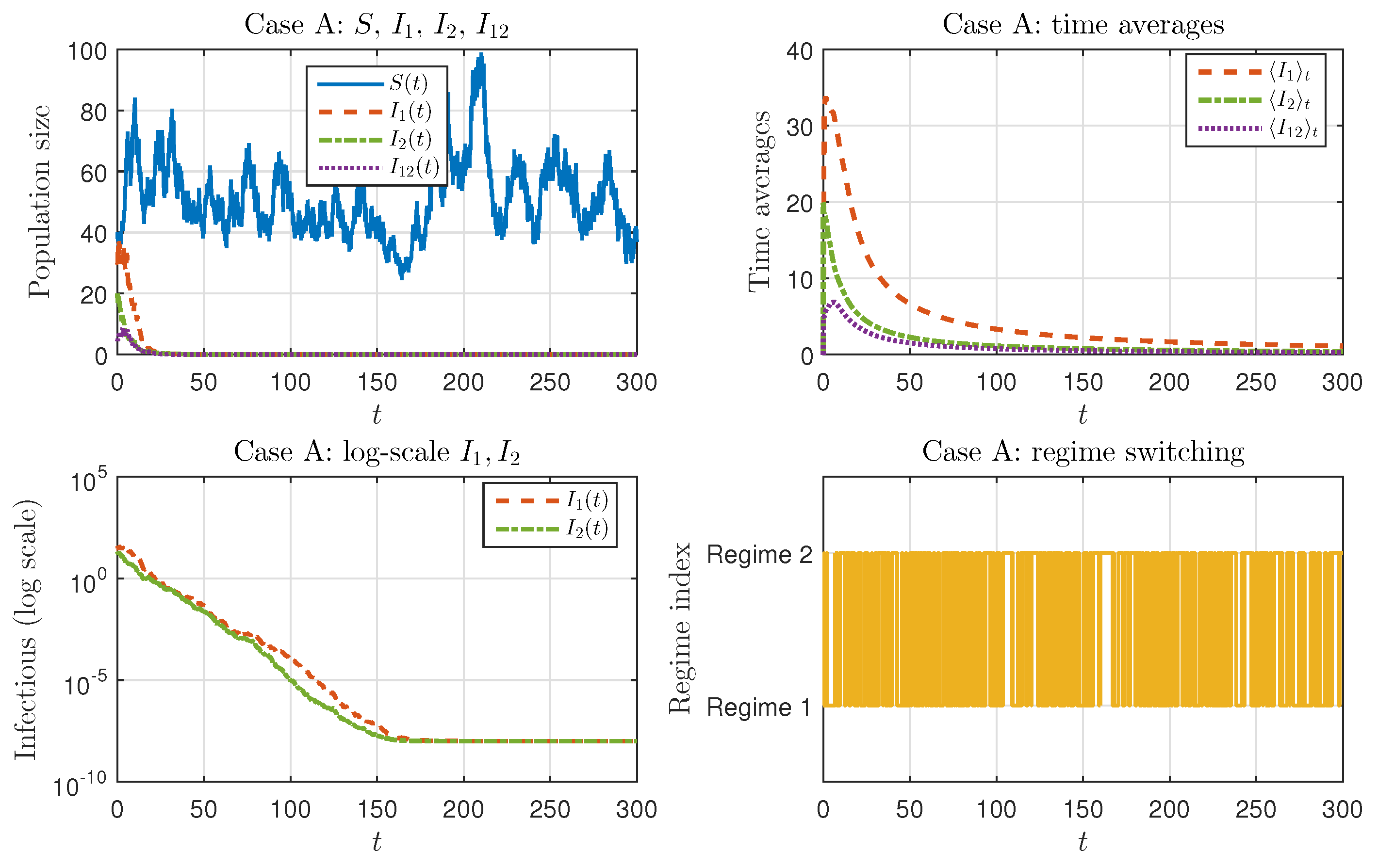
In the first configuration, we take ${\beta }_1\in [0.001,0.003]$ and ${\beta }_2\in [0.001,0.003]$, which yields ${\lambda }_3<0$ and ${\lambda }_4<0$. By Theorem 4, this sign pattern implies almost sure extinction of both primary strains and, consequently, of the co-infected class.

• Biological interpretation of Figure 1. The trajectories indicate a failed invasion scenario. Transmission intensity is below the effective loss intensity generated by (i) natural removal $\mu$, (ii) recovery ${\gamma }_i$, and (iii) disease-induced removal ${\delta }_i$, so each infectious class has a negative net growth when rare. Moreover, the Crowley–Martin denominators amplify this effect by capturing behavioural/contact limitation: even when susceptibles are abundant, effective contacts saturate (via $\kappa S$), and any transient increase in infectious density further reduces marginal transmission (via ${\alpha }_{ij}{I}_j$). Hence, $I_1\left(t\right)$ and $I_2\left(t\right)$ quickly drift towards near-zero levels. Because co-infection requires simultaneous circulation of both strains, the bilinear terms ${\mathrm{\Psi }}_1={\chi }_1{I}_1{I}_2$ and ${\mathrm{\Psi }}_2={\chi }_2{I}_1{I}_2$ collapse even faster, driving $I_{12}\left(t\right)$ to extinction as well. The susceptible compartment relaxes towards the demographic balance $\mathrm{\Lambda }/\mu$, meaning that host turnover dominates and the population remains essentially susceptible in the long run. Table 2 and Table 3 therefore reflect very small time averages, consistent with an elimination regime.

• Case B (persistence of the first strain, extinction of the second).

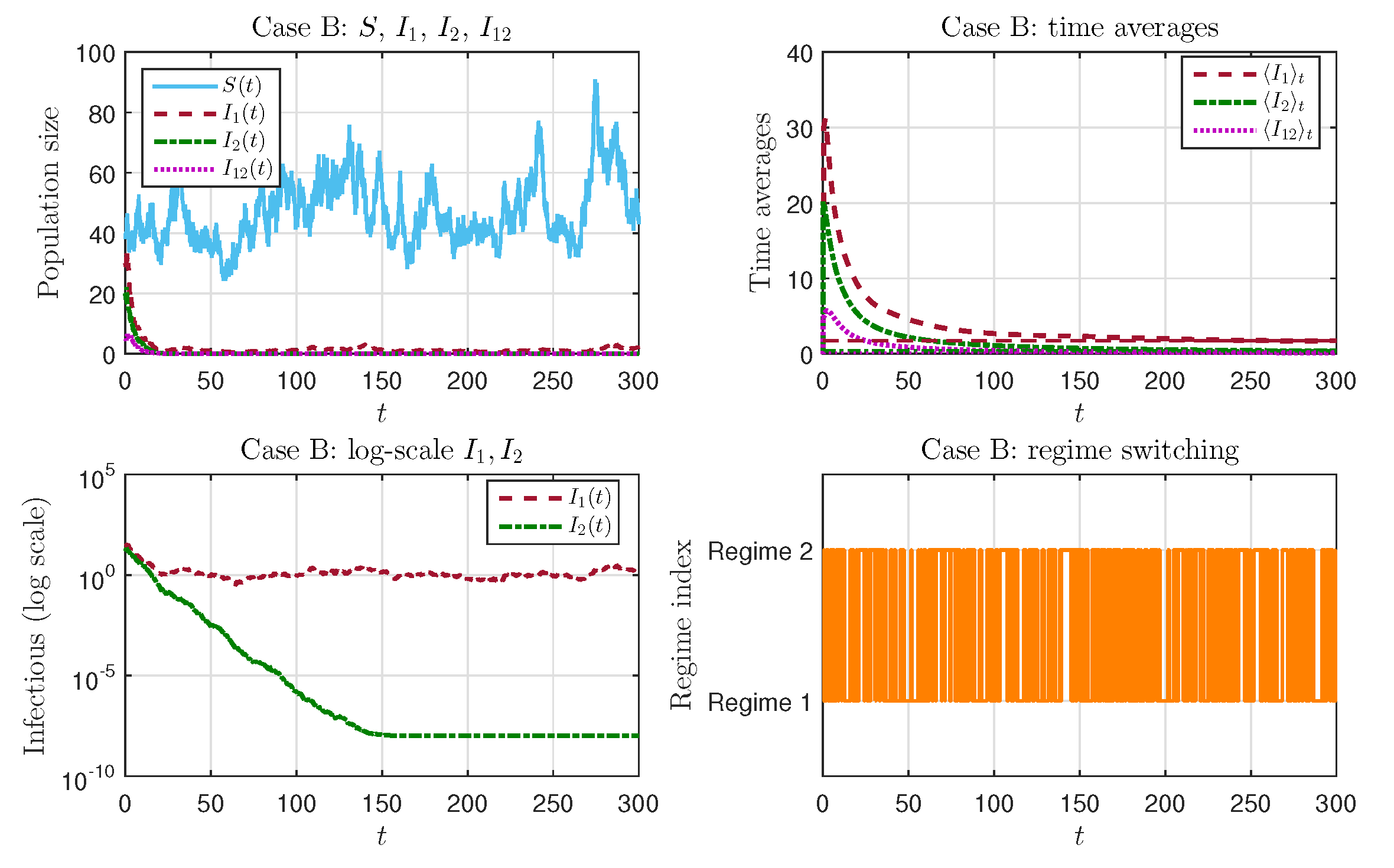
In the second configuration, we increase the transmission rate of strain 1 to ${\beta }_1\in [0.008,0.010]$ while keeping ${\beta }_2\in [0.001,0.003]$. This choice leads to ${\lambda }_2<0<{\lambda }_3$, so Theorem 5 predicts persistence in mean of $I_1$ and extinction in mean of $I_2$, with the co-infected class $I_{12}$ remaining small.

• Biological interpretation of Figure 2. This is a competitive exclusion regime driven by a clear fitness advantage of strain 1. After accounting for recovery and removals $(\mu +{\delta }_1+{\gamma }_1)$ and the saturation effects, strain 1 still achieves a positive long-run growth tendency (captured by the sign condition), so it establishes an endemic level and fluctuates around it under switching/noise. In contrast, strain 2 remains below its invasion threshold: its effective transmission cannot compensate for $(\mu +{\delta }_2+{\gamma }_2)$ and saturation, so $I_2\left(t\right)$ is repeatedly suppressed and spends long epochs near zero. The behaviour of $I_{12}\left(t\right)$ has a direct epidemiological meaning: co-infection is incidence-limited because its inflow is proportional to $I_1{I}_2$. Even though $I_1$ persists, the scarcity of $I_2$ makes co-infection events rare, so $I_{12}\left(t\right)$ shows only small bursts caused by occasional transient excursions of $I_2$. Accordingly, Table 2 and Table 3 exhibits a substantial ${\langle I_1\rangle }_T^{\mathrm{num}}$ with much smaller averages for $I_2$ and $I_{12}$, supporting exclusion in favour of strain 1.

• Case C (persistence of the second strain, extinction of the first).

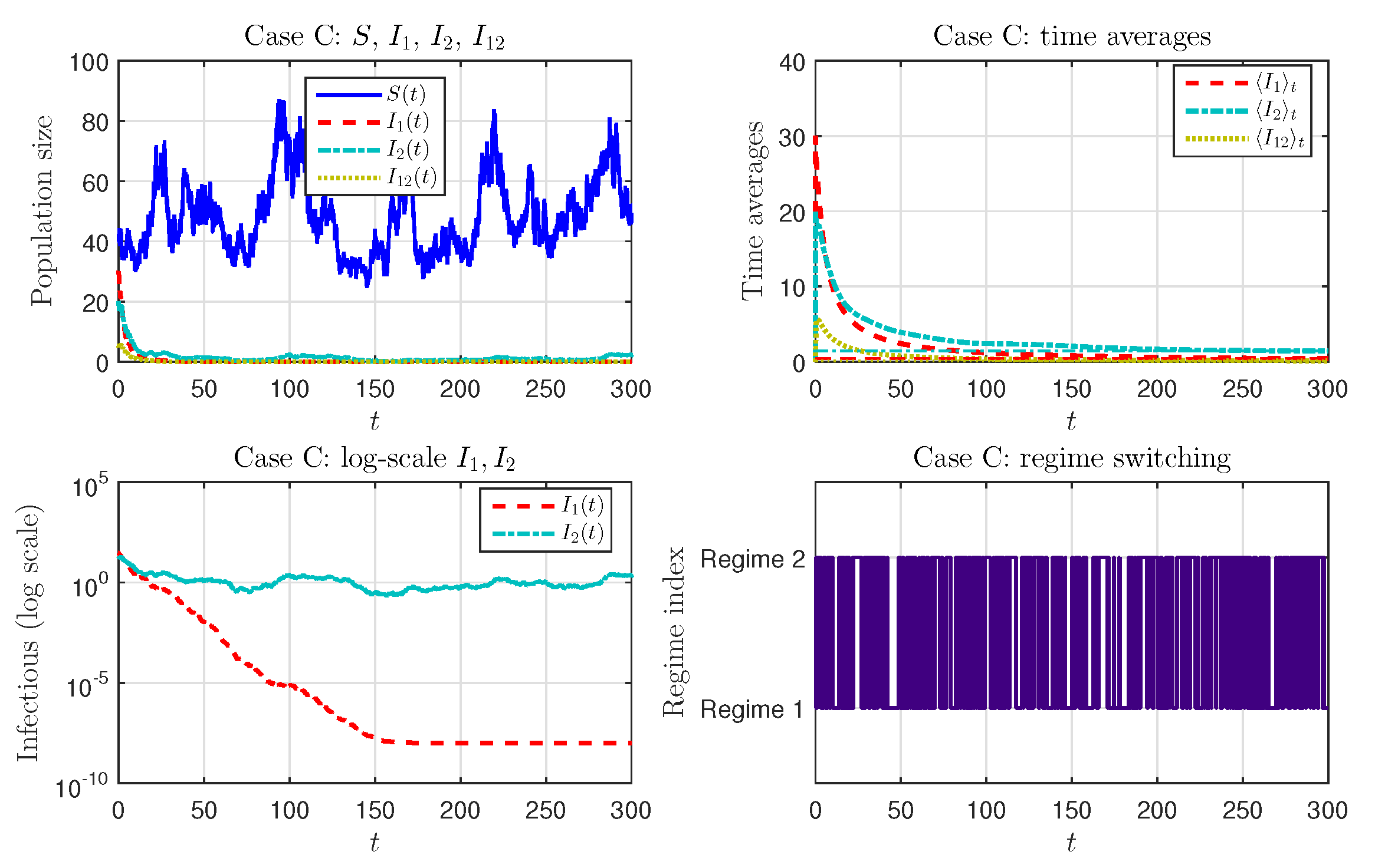
In the third scenario, we take ${\beta }_1\in [0.001,0.003]$ and ${\beta }_2\in [0.008,0.010]$, which yields ${\lambda }_1<0<{\lambda }_4$. The theoretical results predict persistence in mean of $I_2$ and extinction of $I_1$ and $I_{12}$.

• Biological interpretation of Figure 3. Case C is the mirror image of Case B: strain 2 is now the dominant competitor. Its higher baseline transmissibility ${\beta }_2$ allows it to overcome losses $(\mu +{\delta }_2+{\gamma }_2)$ despite the same behavioural and infectious-side saturation. Strain 1 cannot invade and is pushed towards elimination, resulting in long intervals where $I_1\left(t\right)\approx 0$. The co-infected class remains secondary and transient for the same structural reason as in Case B: its creation requires encounters between two actively circulating strains. Thus $I_{12}\left(t\right)$ appears as intermittent, low-amplitude episodes when stochastic fluctuations temporarily lift $I_1$ away from zero, but these episodes do not persist on long horizons. The averages in Table 2 and Table 3 therefore reflect an endemic burden dominated by $I_2$, with negligible contribution from $I_1$ and a small but non-zero contribution from $I_{12}$ capturing transient co-infection events.

• Case D (coexistence in the mean of all infectious classes).

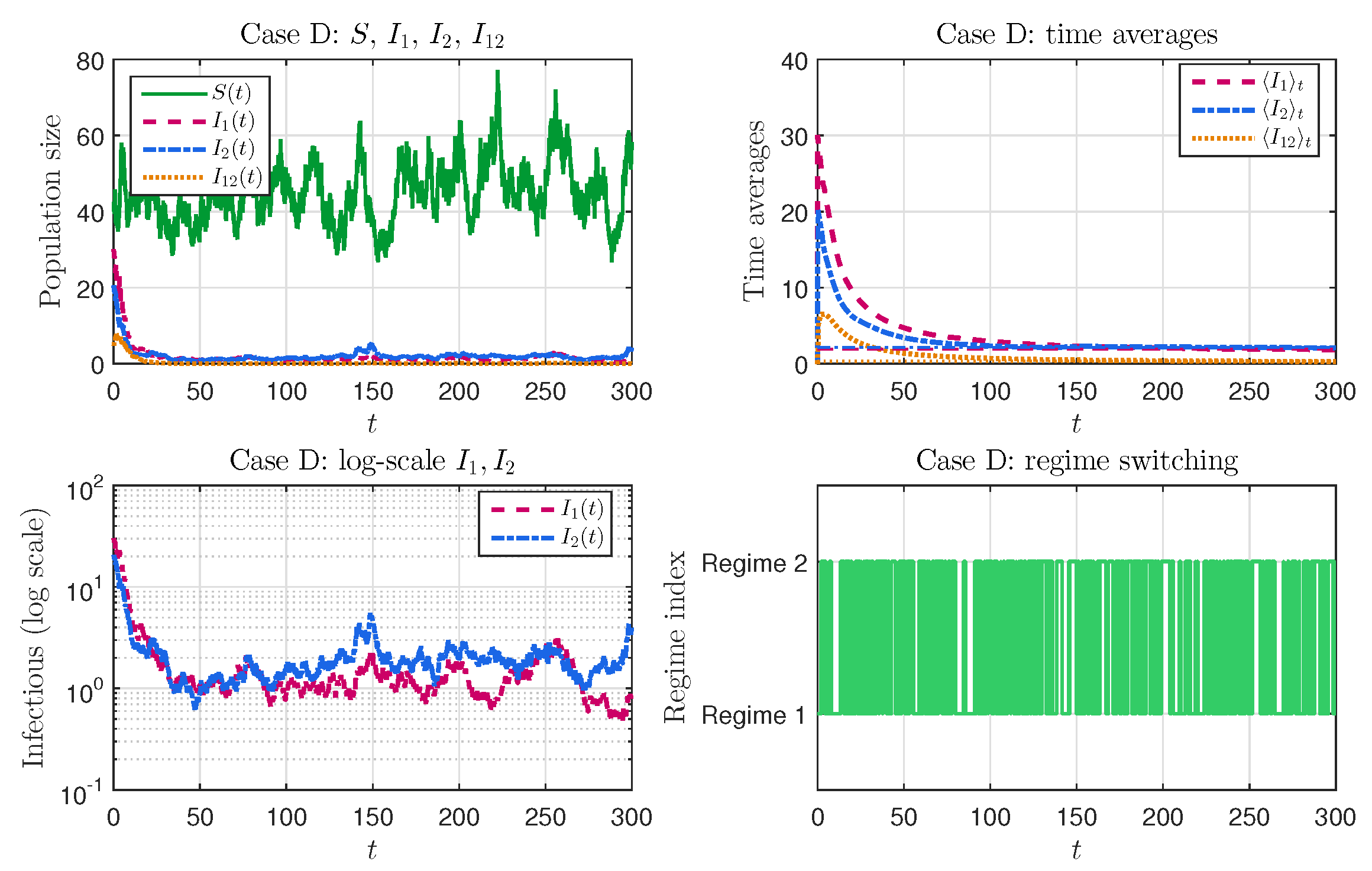
Finally, we select moderately high infection rates ${\beta }_1\in [0.008,0.012]$ and ${\beta }_2\in [0.009,0.013]$, and increase the co-infection intensities to ${\chi }_1={\chi }_2=3\times {10}^{-3}$. In this configuration, we obtain ${\lambda }_i>0$ for $i=1,\dots ,4$, and the coexistence conditions of Theorem 6 are satisfied.

• Biological interpretation of Figure 4. This regime represents long-term co-circulation of both strains together with a persistent co-infected class. Both strains have sufficiently strong effective transmission to compensate for their respective loss rates $(\mu +{\delta }_i+{\gamma }_i)$, even under contact saturation and environmental perturbations. In addition, the larger co-infection coefficients ${\chi }_1,{\chi }_2$ make the conversion $I_1\to I_{12}$ and $I_2\to I_{12}$ epidemiologically relevant whenever both strains are present. Consequently, $I_{12}\left(t\right)$ is not merely a transient by-product but a sustained burden maintained by continual secondary acquisition events. Crowley–Martin saturation plays a stabilising role here: it limits explosive growth during high-transmission phases by reducing marginal incidence at large S and large infectious densities, which supports bounded endemic fluctuations rather than runaway outbreaks. Therefore, the three infectious trajectories in Figure 4 fluctuate around strictly positive levels, and the empirical averages ${\langle I_1\rangle }_T^{\mathrm{num}}$, ${\langle I_2\rangle }_T^{\mathrm{num}}$, and ${\langle I_{12}\rangle }_T^{\mathrm{num}}$ in Table 2 and Table 3 remain clearly bounded away from zero. Epidemiologically, this corresponds to a setting where two variants persist in the same host community, and co-infection contributes a non-negligible fraction of disease burden (e.g., via increased severity or onward transmission).

Generally, the four numerical regimes provide a coherent biological validation of the extinction, single-strain persistence, and coexistence scenarios predicted by the logarithmic Lyapunov analysis. They distinguish (i) failed invasion (Case A), (ii) competitive exclusion (Cases B–C), and (iii) stable co-circulation with sustained co-infection (Case D) under behavioural saturation and hybrid environmental perturbations.

6. Conclusions

In this work, we developed and analysed a hybrid stochastic SIS co-infection model with two primary strains and a co-infected class, driven by Crowley–Martin incidence, Markovian regime switching and multiplicative Lévy perturbations. The model incorporated three distinct sources of complexity that are rarely combined in a single framework: (i) nonlinear behavioural saturation in the transmission mechanism, (ii) explicit co-infection terms coupling the two strains via a shared infected compartment, and (iii) hybrid stochastic forcing through both regime switching and compensated Poisson jumps acting multiplicatively on all epidemiological variables. This setting extended classical deterministic and diffusion-based SIS formulations to a more realistic, yet analytically tractable, description of multi-strain circulation in a fluctuating environment.

At the pathwise level, we first established global existence, uniqueness and positivity of the solution under mild structural assumptions on the parameters and jump amplitudes. By exploiting the specific form of the drift and noise coefficients, we derived a family of logarithmic stochastic differential inequalities for the primary strains and identified noise-corrected growth coefficients ${\lambda }_i$ that incorporated both diffusion and Lévy effects. A key novelty of the analysis lay in the combination of these logarithmic estimates with regime-switching bounds and co-infection structure, which allowed us to control the long-term behaviour of the two primary strains and to show that the co-infected class inherits extinction or persistence properties from the interaction of the primaries.

On this basis, we obtained sharp extinction and persistence-in-mean criteria for the hybrid co-infection system. In particular, we proved that negative upper growth coefficients ${\lambda }_3,{\lambda }_4$ guaranteed almost sure extinction of both primary strains (and hence of the co-infected class), while mixed-sign patterns such as ${\lambda }_2<0<{\lambda }_3$ or ${\lambda }_1<0<{\lambda }_4$ led to single-strain persistence in mean, with the losing strain and the co-infected class becoming negligible over long time intervals. In the fully supercritical regime ${\lambda }_i>0$, $i=1,\dots ,4$, we showed that suitable sign conditions on two auxiliary matrices A and B implied coexistence in mean of both primary strains, and that the co-infected class retained a strictly positive time-averaged burden. To our knowledge, these extinctions, single-strain persistence and coexistence results are the first to be derived for a multi-strain SIS co-infection model with Crowley–Martin incidence under the joint action of regime switching and Lévy jumps.

The theoretical thresholds were supported by a detailed numerical study based on an Euler–Maruyama scheme with jump corrections and a discrete approximation of the Markovian switching process. We implemented four representative parameter regimes corresponding to: (i) double extinction, (ii) persistence of strain 1 and extinction of strain 2, (iii) persistence of strain 2 and extinction of strain 1, and (iv) coexistence in mean of all infectious classes. In each case, the simulated trajectories and empirical time averages of the infectious compartments agreed closely with the sign structure of the noise-corrected growth coefficients ${\lambda }_i$ and the coexistence conditions, thereby providing a coherent numerical validation of the logarithmic Lyapunov analysis. From a biological viewpoint, the four scenarios illustrated the transition from non-invasion to competitive exclusion and long-term co-circulation of two strains in a noisy, regime-switching environment, with the co-infected class behaving as a sensitive marker of mutual interaction between variants.

The methodology developed here can be extended in several directions. On the modelling side, it would be natural to incorporate vaccination, waning immunity or additional epidemiological stages, or to replace the scalar jump process by regime-dependent or state-dependent Lévy measures. On the analytical side, one could investigate finer distributional properties (e.g., ergodicity and invariant measures in the coexistence regime) or derive large-deviation estimates for rare extinction events in the supercritical case. These perspectives underline that the hybrid stochastic co-infection framework introduced in this paper provides a flexible platform for studying multi-strain dynamics under realistic environmental and behavioural variability, and offers a tractable set of threshold quantities that remain robust in the presence of both regime switching and jump noise.