Carbon Convenience Yields and Probability Density Forecasts for Carbon Returns

Abstract

We explore the role of carbon convenience yields in forecasting the probability density of carbon returns. While theory suggests that convenience yields contain forward-looking information, their predictive content for carbon returns—especially in a density forecasting framework—remains underexplored. We propose a probability density forecasting approach that combines a mixed data sampling (MIDAS) regression with a non-parametric bootstrap and kernel density estimation. Using data from the European carbon market, we find that convenience yields significantly predict carbon returns. It takes approximately 19 days for a disturbance in carbon convenience yields to affect carbon returns, with the impact persisting for around 27 days. Moreover, our approach outperforms existing benchmark models in predicting the probability density of carbon returns, showing superior predictive accuracy and robustness.

1. Introduction

In response to the growing urgency of climate change, carbon emission trading systems have been widely adopted as market-based instruments to reduce greenhouse gas emissions [1,2,3,4,5]. Since its launch, the European Union Emissions Trading System (EU ETS) has established carbon allowances as tradable assets, granting the right to emit one metric tonne of carbon dioxide or its equivalent [6,7,8]. Regulated firms must surrender sufficient allowances to cover their verified emissions, while financial investors also participate in the market for speculative and diversification purposes [9,10,11,12]. As a result, carbon allowances have evolved into an actively traded commodity with increasing financial relevance.

Despite the rapid development of the EU ETS, carbon prices exhibit substantial volatility, posing challenges for market participants and policymakers. Carbon prices reflect marginal abatement costs and play a central role in guiding emission reduction decisions [13,14]. Accurate forecasts of carbon prices or returns are therefore essential for risk management, investment decisions, and policy evaluation. However, forecasting carbon prices remains difficult due to market complexity, nonlinear dynamics, and structural changes [15,16,17]. Existing studies have documented that carbon prices are influenced by a range of factors, including energy prices, macroeconomic conditions, and weather-related variables [18,19,20,21,22], which have been widely used as predictors in empirical forecasting models [5,18,23,24].

Compared with these traditional determinants, the role of carbon convenience yields has received relatively limited attention. The convenience yield reflects the implicit benefit of holding physical carbon allowances rather than futures contracts, capturing firms’ incentives to maintain inventories in the presence of compliance obligations and allowance banking [25,26,27,28]. As a key concept in commodity pricing theory, convenience yields convey information about market tightness and inventory conditions, and may therefore contain valuable predictive information for carbon returns [29,30,31,32,33]. Whether and how carbon convenience yields can be exploited to improve the forecasting of carbon returns remains an open empirical question.

At the same time, the existing literature on carbon price forecasting has largely focused on point forecasts, while relatively little attention has been paid to probability density forecasts [34]. Density forecasts provide a full characterization of future uncertainty, offering information beyond single-point predictions and allowing market participants to assess risks under different scenarios [35,36,37,38,39,40,41]. Such forecasts are particularly relevant for carbon markets, where regulatory interventions and demand fluctuations may generate asymmetric risks.

Motivated by these considerations, this paper investigates whether carbon convenience yields can improve both point and density forecasts of carbon returns in the EU ETS. We employ mixed data sampling (MIDAS) regressions to link weekly carbon returns with daily carbon convenience yields, allowing us to exploit high-frequency information while maintaining the practical relevance of weekly forecasts [42,43,44]. Building on the MIDAS-based point forecasts, we further construct probability density forecasts using a nonparametric bootstrap and kernel density estimation framework, which accommodates parameter uncertainty without imposing strong distributional assumptions [45].

Using December futures contracts in the EU ETS over the period from 8 February 2008 to 29 December 2023, we document that carbon convenience yields contain economically and statistically significant predictive information for weekly carbon returns. The MIDAS model incorporating convenience yields outperforms a broad set of benchmark models, including alternative MIDAS specifications based on energy and stock market variables, conventional time-series models (e.g., ARDL, ARIMA, and GARCH), and machine learning approaches (e.g., RF and LSTM). Moreover, the resulting density forecasts exhibit satisfactory calibration. These findings are robust to adjustments for carbon convenience yields, subsample selection, alternative bootstrap schemes.

The main contributions of this paper are twofold. First, it extends research on the determinants of carbon returns by highlighting the predictive role of carbon convenience yields, a key concept in commodity pricing that has been underexplored in the context of carbon markets [46,47]. Second, it enriches the carbon forecasting literature by providing probability density forecasts of carbon returns that leverage the role of carbon convenience yields. This offers a more comprehensive assessment of uncertainty that is relevant for both policymakers and market participants.

The remainder of this paper is structured as follows: Section 2 introduces the methodology. Section 3 describes the data. Section 4 presents the empirical results for point and density forecasts, along with robustness checks. Finally, Section 5 concludes this paper.

2. Methodology

2.1. The Theory of Storage

Since the convenience yield is not directly observable, it is typically inferred using the theory of storage [31,32,33]. Under the absence of arbitrage, the futures price should equal the spot price adjusted for carry costs, which include the forgone interest rate and storage costs, and the net of the convenience yield. This relationship can be expressed as:

$$F_{t,T}=S_t{e}^{r{f}_{t\to T}+s{c}_{t\to T}-c{y}_{t\to T}},$$

(1)

where $F_{t,T}$ denotes the price of a carbon futures contract at time t with maturity T, and $S_t$ is the spot price at time t. The terms $r{f}_{t\to T}$, $s{c}_{t\to T}$, and $c{y}_{t\to T}$ represent the risk-free interest rate, storage cost, and convenience yield over the period from t to T, respectively. Although carbon allowances do not incur physical storage costs, transaction and holding costs exist. Accordingly, we define the net convenience yield as $y_{t\to T}=c{y}_{t\to T}-s{c}_{t\to T}$, which is the main variable of interest in this study.

Given the localized nature of carbon spot markets and the global reach of futures markets that assist investors in price discovery and risk sharing, we infer carbon net convenience yields from carbon futures, following the tradition to calculate commodity net convenience yields [30,47]. Denote $F_{t,T_1}$ as the price of a future contract maturing at time $T_1$ (with $T_1>T$). According to Equation (1),

$$F_{t,T_1}=S_t{e}^{r{f}_{t\to T_1}-y_{t\to T_1}}=S_t{e}^{r{f}_{t\to T}-y_{t\to T}}{e}^{r{f}_{T\to T_1}-y_{T\to T_1}}=F_{t,T}{e}^{r{f}_{T\to T_1}-y_{T\to T_1}},$$

(2)

where $r{f}_{T\to T_1}$ and $y_{T\to T_1}$ refer to the interest rate and net convenience yield at time t for the period from time T to $T_1$. Consequently, the carbon (net) convenience yield is defined as:

$$y_{T\to T_1}=ln\left({\displaystyle \frac{F_{t,T}}{F_{t,T_1}}}\right)+r{f}_{T\to T_1}.$$

(3)

The term $ln\left({\displaystyle \frac{F_{t,T}}{F_{t,T_1}}}\right)$ is commonly referred to as the basis for carbon futures [30].

2.2. The Definition of Carbon Returns

We focus on forecasting carbon returns rather than prices, as returns mitigate nonstationarity concerns while preserving economically relevant information [44]. Given that carbon futures account for more than 80% of trading activity in the EU ETS, we analyze futures returns defined as:

$$r_{t+1}={\displaystyle \frac{F_{t+1,T}}{F_{t,T}}}-1\approx ln\left({\displaystyle \frac{F_{t+1,T}}{F_{t,T}}}\right),$$

(4)

where $r_{t+1}$ denotes the simple return from time t to $t+1$ on a futures contract maturing at time T. This return corresponds to the excess return on a fully collateralized futures position, as no initial payment is required when entering a futures contract. As shown in Equation (4), the simple return provides a close approximation to the log return. This approximation is justified because the futures price ratio $F_{t+1,T}/F_{t,T}$ is typically close to one, implying that higher-order terms in the log expansion are negligible [30].

2.3. Methods for Probability Density Forecasts

2.3.1. MIDAS Regression Models

The MIDAS model has demonstrated strong performance in handling mixed-frequency variables related to financial markets [42], though its application to the carbon market has been limited. Recently, Zhao et al. [43] and Han et al. [44] have introduced this model to the analysis of carbon prices, highlighting its strong suitability for predicting carbon prices. The $MIDAS(h,p,q)$ model is defined as:

$$r_t=\alpha +\sum _{j=1}^p{\gamma }_j{r}_{t-j}+\beta W\left(L^{1/m},\theta \right)y_{t-h/m}^{\left(m\right)}+{ϵ}_t,$$

(5)

where $r_t$ denotes weekly carbon return as defined in Equation (4), $\alpha$, $\gamma$, and $\beta$ are parameters to be estimated, p is the maximum lag order for carbon returns, and $y_{t-h/m}^{\left(m\right)}$ refers to the daily carbon convenience yield, which can be observed m times a week. Thus, we set $m=5$ in this paper. The term h represents the number of step ahead. In particular, $h=1$ suggests that we use the daily carbon convenience yields up to Thursday in week t to explain the carbon return in that week. Practically, at the time somewhere in week t, we aim to predict the carbon return in week $t+1$. Therefore, we set $h\ge 5$ in this paper. The term $W\left(L^{1/m},\theta \right)$ is decided by a parameter vector with limited dimension $\theta$ and a lag operator $L^{1/m}$, where $L^{k/m}{y}_{t-h/m}^{\left(m\right)}=y_{t-h/m-k/m}^{\left(m\right)}$. Accordingly, $W\left(L^{1/m},\theta \right)={\sum }_{k=0}^{q}w\left(k,\theta \right)L^{k/m}$, where $w\left(k,\theta \right)$ is a polynomial weight, and q is the maximum lag order of carbon convenience yields.

Regarding the polynomial weight, we explore six different specifications to identify the one that best captures the influence of carbon convenience yields on carbon returns. Particularly, we consider the Beta polynomial weight, which is defined as $w\left(k,\theta \right)=w\left(k,{\theta }_1,{\theta }_2\right)={\displaystyle \frac{f\left(k/q,{\theta }_1,{\theta }_2\right)}{{\sum }_{k=1}^{q}f\left(k/q,{\theta }_1,{\theta }_2\right)}}$, given that $f\left(k/q,{\theta }_1,{\theta }_2\right)={(k/q)}^{\left({\theta }_1-1\right)}{\left(1-k/q\right)}^{\left({\theta }_2-1\right)}{\displaystyle \frac{\Gamma \left({\theta }_1+{\theta }_2\right)}{\left(\Gamma \left({\theta }_1\right)\Gamma \left({\theta }_2\right)\right)}}$ and $\Gamma \left(\theta \right)={\int }_0^{\infty }{e}^{-x}{x}^{\theta -1}dx$. The BetaNN polynomial weight is defined as $w\left(k,\theta \right)=w\left(k,1,{\theta }_2,{\theta }_3\right)={\displaystyle \frac{f\left(k/q,1,{\theta }_2\right)}{{\sum }_{k=1}^{q}f\left(k/q,1,{\theta }_2\right)}}+{\theta }_3$, where $f\left(k/q,1,{\theta }_2\right)={\left(1-k/q\right)}^{\left({\theta }_2-1\right)}{\displaystyle \frac{\Gamma \left(1+{\theta }_2\right)}{\left(\Gamma \left(1\right)\Gamma \left({\theta }_2\right)\right)}}$ and $\Gamma \left(\theta \right)={\int }_0^{\infty }{e}^{-x}{x}^{\theta -1}dx$. Additionally, the Almon lag polynomial is described as $\beta w\left(k,\theta \right)={\sum }_{j=0}^J{\theta }_j{k}^j$ and the exponential Almon lag polynomial is defined as $w\left(k,\theta \right)={\displaystyle \frac{e^{\left({\theta }_{1}k+{\theta }_2{k}^2+\cdots +{\theta }_J{k}^J\right)}}{{\sum }_{k=1}^q{e}^{\left({\theta }_{1}k+{\theta }_2{k}^2+\cdots +{\theta }_J{k}^J\right)}}}$. The polynomial specification with step function refers to $\beta w\left(k,\theta \right)={\theta }_1{I}_{i\in \left[a_0,a_1\right]}+{\sum }_{j=2}^J{\theta }_j{I}_{i\in \left[a_{j-1},a_j\right]}$, where $a_0=1<a_1<\dots <a_J=q$, and $I_{i\in \left[a_{j-1},a_j\right]}=1$ if $a_{j-1}\le i\le a_j$. Otherwise, $I_{i\in \left[a_{j-1},a_j\right]}=0$. Finally, we also consider the unrestricted MIDAS (U-MIDAS) polynomial weights, which is defined as $\beta W\left(L^{1/m},q,\theta \right)x_{t-h}^{\left(m\right)}={\sum }_{k=0}^q{\beta }_k{x}_{t-h-k/m}^{\left(m\right)}$.

2.3.2. Non-Parametric Bootstrap Process

To construct probability density forecasts for carbon returns, we employ a non-parametric bootstrap procedure based on the estimated MIDAS model introduced in Section 2.3.1. The bootstrap allows us to account for parameter uncertainty without imposing parametric assumptions on the distribution of innovations [45,48].

In the baseline analysis, we apply an i.i.d. residual bootstrap. This choice is motivated by the specification of the MIDAS regression model, which explicitly incorporates lagged carbon returns as regressors. By conditioning on past returns, the MIDAS framework captures the dominant serial dependence in carbon returns, thereby substantially mitigating autocorrelation in the regression residuals. As a result, the remaining error terms are approximately serially uncorrelated, making the i.i.d. bootstrap a reasonable and commonly adopted approach in density forecasting applications based on dynamic regression models [45,48]. Specifically, after estimating the MIDAS model in Equation (5), we generate bootstrap samples by resampling the regression residuals with replacement from their empirical distribution. The bootstrap recursion is given by:

$$r_t^{\ast }=\widehat{\alpha }+\sum _{j=1}^p{\widehat{\gamma }}_j{r}_{t-j}^{\ast }+\widehat{\beta }W\left(L^{1/m},\widehat{\theta }\right)y_{t-h/m}^{\left(m\right)}+{ϵ}_t^{\ast },$$

(6)

where $r_t^{\ast }=r_t$ for $t=1,\dots ,p$ serve as initial values. The parameters $\widehat{\alpha }$, ${\widehat{\gamma }}_j$, $\widehat{\beta }$, and $\widehat{\theta }$ are estimated from the original sample, and ${ϵ}_t^{\ast }$ is drawn with replacement from the empirical distribution of the residuals.

To generate out-of-sample forecasts, we iterate:

$${\widehat{r}}_{T+i}^{\ast }={\widehat{\alpha }}^{\ast }+\sum _{j=1}^p{\widehat{\gamma }}_j^{\ast }{r}_{T+i-j}^{\ast }+{\widehat{\beta }}^{\ast }W\left(L^{1/m},{\widehat{\theta }}^{\ast }\right)y_{T+i-h/m}^{\left(m\right)}+{ϵ}_{T+i}^{\ast },$$

(7)

where ${\widehat{\alpha }}^{\ast }$, ${\widehat{\gamma }}_j^{\ast }$, ${\widehat{\beta }}^{\ast }$, and ${\widehat{\theta }}^{\ast }$ denote the bootstrap estimates for each iteration using training sample $\left\{r_1^{\ast },\cdots ,r_T^{\ast }\right\}$. In the bootstrap prediction process, we consider an error term ${ϵ}_{T+i}^{\ast }$ in order to capture the nonlinear effects not explicitly modeled by the linear MIDAS specification, following the practice of Han et al. [44]. The error term ${ϵ}_{T+i}^{\ast }$ is resampled from the empirical distribution of the residuals presented in Equation (5) for the test sample. In this paper, we replicate this procedure 9999 times to obtain a distribution of forecasted returns at each horizon.

Nevertheless, we acknowledge that carbon returns may still exhibit residual temporal dependence or conditional heteroskedasticity that is not fully absorbed by the linear MIDAS specification. To address this concern, we conduct robustness checks using a block bootstrap that preserves the time-series dependence structure of the residuals.

2.3.3. Kernel Density Estimation

Based on the bootstrap forecasts, we estimate the predictive density of carbon returns using kernel density estimation. Let ${\widehat{r}}_{T+i,1}^{\ast },\dots ,{\widehat{r}}_{T+i,n}^{\ast }$ denote the bootstrap forecasts at time $T+i$, with $n=9999$. The predictive density is given by:

$${\widehat{f}}_{b,T+i}\left(x\right)={\displaystyle \frac{1}{n}}\sum _{j=1}^n{K}_b(x-{\widehat{r}}_{T+i,j}^{\ast })={\displaystyle \frac{1}{nb}}\sum _{j=1}^n{K}_b\left({\displaystyle \frac{x-{\widehat{r}}_{T+i,j}^{\ast }}{b}}\right),$$

(8)

where b is the bandwidth parameter and $K(·)$ is the kernel function. We employ the Gaussian kernel, $K\left(u\right)={\displaystyle \frac{1}{\sqrt{2\pi }}}{e}^{-u^2/2}$, which is widely used in empirical density forecasting [41]. Robustness checks with alternative bandwidth rules and kernel choices are reported in Section 4.

2.4. Forecast Evaluation Metrics

Point forecast accuracy is evaluated using the root mean squared error (RMSE), mean squared error (MSE), and mean absolute error (MAE), defined as

$$\mathrm{RMSE}=\sqrt{{\displaystyle \frac{1}{N}}\sum _{t=1}^N{(r_t-{\widehat{r}}_t)}^2},\mathrm{MSE}={\displaystyle \frac{1}{N}}\sum _{t=1}^N{(r_t-{\widehat{r}}_t)}^2,\mathrm{MAE}={\displaystyle \frac{1}{N}}\sum _{t=1}^N|r_t-{\widehat{r}}_t|.$$

(9)

To formally compare predictive accuracy across competing models, we employ the Diebold–Mariano (DM) test based on squared forecast errors. For density forecasts, we use the log predictive score and the continuous ranked probability score (CRPS), which are proper scoring rules widely adopted in the density forecasting literature. These measures jointly assess sharpness and calibration of the predictive densities.

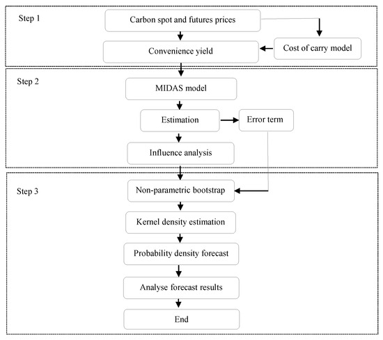
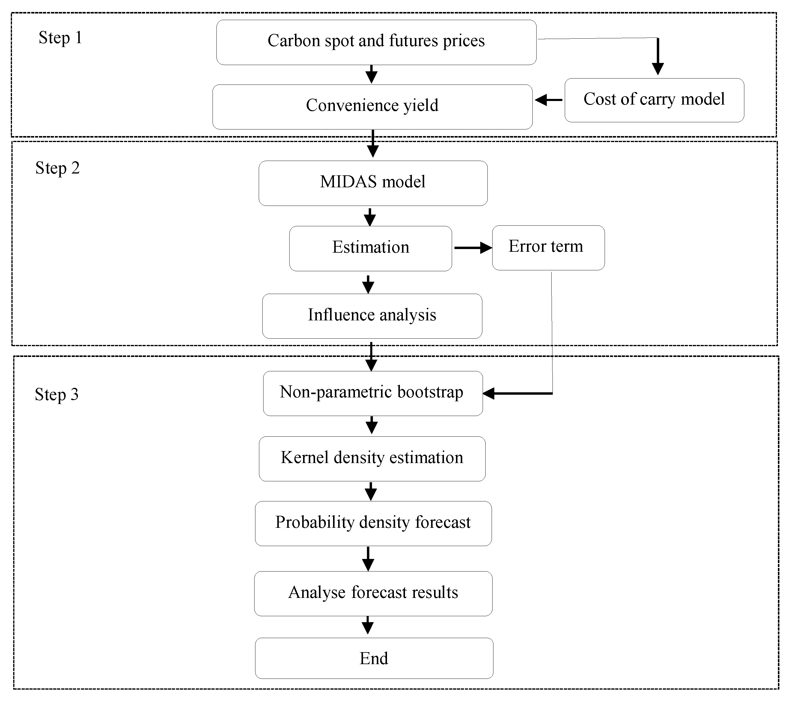
Generally, this paper primarily explores the impact of carbon convenience yields on carbon returns and subsequently provides probability predictions for these returns. The methodology encompasses three distinct steps, as depicted in Figure 1.

Figure 1. The flow chart for the probability density forecasts for carbon returns.

3. Data

3.1. Data Sources

This paper focuses on forecasting carbon returns associated with December futures contracts traded on the Intercontinental Exchange (ICE). We deliberately concentrate on December-maturity contracts because they are by far the most actively traded and liquid instruments in the EU ETS futures market, consistently exhibiting substantially higher trading volumes and open interest than contracts with other maturities. Futures with alternative maturities are thinly traded for most of the sample period, rendering their prices less informative and potentially noisy. As a result, December futures are widely regarded as the benchmark contracts for price discovery in the European carbon market [2,27].

To construct a continuous series of December futures prices, we follow the standard rollover procedure commonly adopted in the commodity futures literature [30,49]. Specifically, we assume that investors roll over their December futures positions by the end of October each year, approximately four to six weeks before contract expiration. This assumption reflects the market practice that financial participants generally avoid physical delivery of carbon allowances and tend to close or roll positions ahead of maturity, a period often associated with elevated price volatility. Based on this rollover scheme, carbon convenience yields are inferred from the first- and second-nearby December futures prices.

To assess whether carbon convenience yields provide incremental predictive information beyond conventional determinants, we also consider a set of established control variables commonly used in the carbon pricing literature. For energy markets, we include futures prices of crude oil, coal, and natural gas, which are key drivers of emissions and abatement costs in Europe. Specifically, we use Brent crude oil futures, Rotterdam coal futures, and UK natural gas futures traded on ICE. For the stock market, we employ Euro Stoxx 50 futures traded on Eurex, which effectively capture broader European macroeconomic and financial conditions. These daily continuous futures prices are constructed by rolling contracts across all available maturities at least two months prior to expiration. These variables are incorporated into alternative MIDAS specifications as benchmark models to conduct a systematic comparison with convenience-yield-based forecasts.

Carbon returns are computed as simple weekly returns based on the nearest-to-maturity December futures contract, as defined in Equation (4). Weekly prices are sampled on a Friday-to-Friday basis. If the end-of-week price is unavailable due to market holidays, we use the most recent available trading-day closing price as a proxy. This procedure preserves the weekly frequency while minimizing data loss and is standard in empirical studies using futures prices.

Weekly and daily futures price data are obtained from the Commodity Research Bureau (CRB). For the risk-free interest rate, we employ the Euro LIBOR rate obtained from the Wind database. Equation (3) defines the carbon (net) convenience yield as a daily expected annual rate (December-December). Accordingly, we use the annualized LIBOR rate of the corresponding horizon for the daily calculation.

The sample period spans from 8 February 2008, to 29 December 2023. Following the forecasting literature [3], we set 6 November 2020 as the breakpoint to divide the sample into an in-sample (training) period and an out-of-sample (testing) period. Approximately 80% of the observations are used to estimate the models described in Section 2, while the remaining 20% are reserved for evaluating out-of-sample predictive performance.

3.2. Data Description

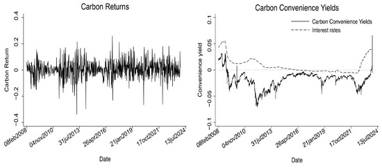
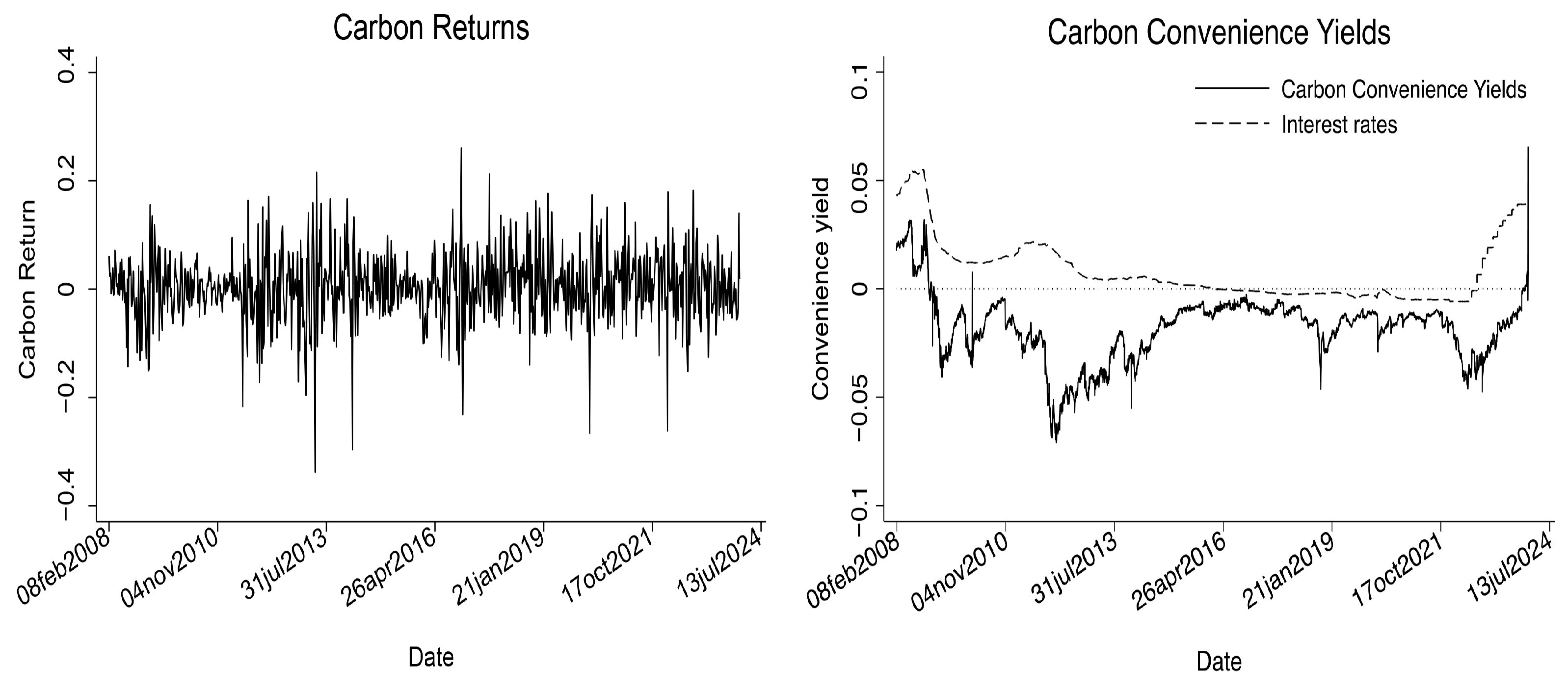
Table 1 reports the summary statistics for carbon returns, carbon convenience yields, and other explanatory variables, while Figure 2 illustrates their time-series behavior. The average weekly return on December futures is 0.346%, corresponding to an annualized return of approximately 16%. This relatively high return highlights the attractiveness of carbon allowances as an investment asset and is consistent with the increasing participation of financial investors in the EU ETS, as reflected in the rapid growth of futures trading volume [10,14]. At the same time, carbon returns exhibit substantial volatility, with a standard deviation of 6.504% and a wide range from −33.753% to 26.061%, underscoring the considerable risk faced by market participants.

Table 1. Summary statistics of carbon returns and carbon convenience yields (%).

Variables	Mean	Std. Dev	Min	Max	ADF	Obs.
r	0.346	6.504	−33.753	26.061	−28.926 ***	830
y	−1.803	1.538	−7.080	6.581	−2.980 **	4151
$oil$	0.023	2.161	−22.917	14.710	−66.091 ***	4151
$coal$	0.041	2.545	−20.864	49.530	−54.943 ***	4151
$gas$	−0.066	3.356	−30.041	47.780	−60.750 ***	4151
$stock$	0.027	1.413	−11.308	12.051	−65.280 ***	4151

Note: This table reports the summary statistics of carbon returns and carbon convenience yields. r refers to the carbon returns on December futures contracts on a weekly basis; y refers to carbon convenience yields on a daily basis. ** and *** represent significance at 5% and 1% level, respectively.

Figure 2. The fluctuations of carbon returns and carbon convenience yields.

To ensure the validity of the subsequent time-series analysis, we conduct unit root tests for all return and convenience yield series. Specifically, we apply the Augmented Dickey–Fuller (ADF) test. As reported in Table 1, the null hypothesis of a unit root is rejected for carbon returns, carbon convenience yields, and all control variables at the 1% or 5% significance level, confirming that the series used in the empirical analysis are stationary.

Regarding carbon convenience yields, as defined in Section 3.1, they are inferred from the price spread between the first- and second-nearby December futures contracts and represent the expected net convenience yield from holding carbon allowances over a December–December horizon. Table 1 shows that the average annualized carbon convenience yield is −1.804%, consistent with the findings of Palao and Pardo [27]. Figure 2 further illustrates that convenience yields are predominantly negative throughout the sample period, turning persistently negative after 2009. Additionally, these yields consistently fall below interest rates, indicating a persistently contangoed state in the carbon futures market, thereby rendering the holding of carbon allowances inconvenient for investors [27]. This prevalence of negative convenience yields and persistent contango in the EU ETS futures market can be attributed to several structural features of the carbon market. First, generous allowance allocations and banking rules, particularly during earlier regulatory phases, led to a persistent surplus of allowances, reducing the scarcity value of holding inventories. Second, compliance obligations are annual, implying that regulated firms have limited incentives to hold allowances continuously throughout the year, as long as sufficient allowances are available at the submission deadline [21]. Third, financial investors, who are not subject to compliance requirements, generally prefer futures contracts over spot holdings due to lower transaction costs and the absence of storage or administrative burdens [12]. Together, these factors weaken the benefits of holding physical allowances relative to futures positions, resulting in negative net convenience yields that remain below prevailing interest rates.

4. Results

4.1. Point Predictions with the Influence of Carbon Convenience Yields

Since probability density forecasts critically depend on accurate point predictions, we first evaluate the point forecasting performance of MIDAS models incorporating carbon convenience yields. This section proceeds in three steps. First, we determine the optimal MIDAS specification for convenience yields across different forecast horizons. Second, we analyze the dynamic effects implied by the optimal model. Third, we conduct a comprehensive horse race against both traditional econometric benchmarks and machine learning models, supplemented by formal predictive comparison tests.

As discussed in Section 2.3.1, the specification of MIDAS models—including lag orders, step ahead, and weighting schemes—plays a crucial role in forecasting performance [44]. Rather than fixing these elements a priori, we adopt a data-driven approach. Specifically, we evaluate six polynomial weighting schemes to identify which best captures the relationship between carbon convenience yields and returns. To determine the optimal maximum lag orders for the convenience yields (q) and carbon returns (p), we consider values from 1 to 60 days ($1\le q\le 60$) and from 0 to 9 weeks ($0\le p\le 9$), respectively. For the forecast step ahead (h), which reflects the sensitivity of carbon returns to changes in convenience yields [44], we consider a range from 5 to 20 days ($5\le h\le 20$). This range is chosen because our objective is to forecast the following week’s return using the most current yield data—a practical focus for investors. For a given forecast horizon h, we first select the best-performing MIDAS specification based on the root mean squared error (RMSE) in the out-of-sample period. RMSE is widely used in the carbon price forecasting literature as a robust measure of predictive accuracy [3,15,18].

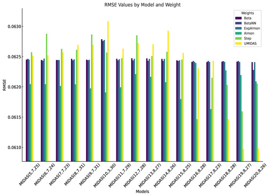
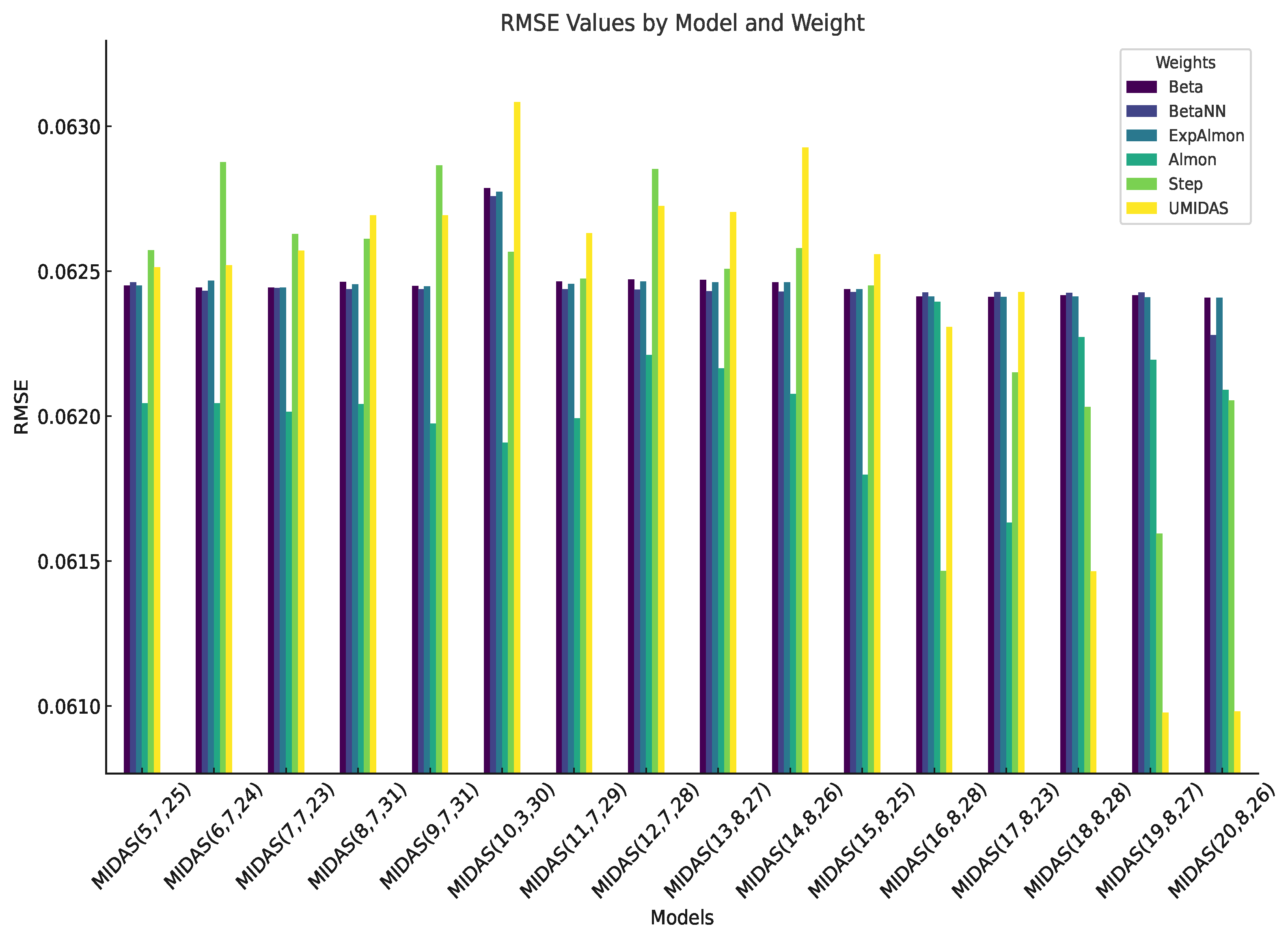
Table 2 illustrates the model selection procedure under $h=5$ as an example. Across different lag orders for carbon returns, the $Almon\text{-}MIDAS(5,7,25)$ model performs best under the condition with $h=5$. Furthermore, Figure 3 effectively illustrates the RMSE variations among the top-performing MIDAS models with different polynomial weights under each conditions with different step ahead (h). We find that polynomial weights do have, to some degree, influence on the prediction accuracy of MIDAS models, while the influence is relatively modest. This insight underscores the importance of evaluating all polynomial weights to select the most suitable one under varying conditions, rather than predetermining a specific weight.

Table 2. RMSEs of $MIDAS(h,p,q)$ models under the condition of h = 5.

Weights	Lag Order for Convenience Yields (q)				Lag Order for Convenience Yields (q)
	5	25	40	60	5	25	40	60
	$p=0$				$p=1$
$Beta$	0.06296	0.06296	0.06296	0.06296	0.06305	0.06305	0.06305	0.06305
$BetaNN$	0.06297	0.06298	0.06295	0.06296	0.06306	0.06308	0.06304	0.06305
$ExpAlmon$	0.06296	0.06296	0.06296	0.06296	0.06305	0.06305	0.06305	0.06305
$Almon$	0.06295	0.06233	0.06282	0.06294	0.06305	0.06241	0.06296	0.06303
$Step$	0.06300	0.06288	0.06292	0.06335	0.06311	0.06303	0.06309	0.06357
$UMIDAS$	0.06290	0.06296	0.06321	0.06414	0.06301	0.06302	0.06324	0.06418
	$p=2$				$p=3$
$Beta$	0.06286	0.06286	0.06286	0.06286	0.06277	0.06277	0.06277	0.06277
$BetaNN$	0.06286	0.06284	0.06280	0.06285	0.06277	0.06279	0.06276	0.06277
$ExpAlmon$	0.06286	0.06286	0.06286	0.06286	0.06277	0.06277	0.06277	0.06277
$Almon$	0.06281	0.06216	0.06272	0.06283	0.06271	0.06205	0.06267	0.06274
$Step$	0.06290	0.06273	0.06282	0.06331	0.06279	0.06268	0.06278	0.06330
$UMIDAS$	0.06278	0.06270	0.06295	0.06375	0.06266	0.06259	0.06277	0.06366
	$p=4$				$p=5$
$Beta$	0.06285	0.06285	0.06285	0.06285	0.06281	0.06281	0.06281	0.06281
$BetaNN$	0.06285	0.06283	0.06284	0.06285	0.06281	0.06280	0.06280	0.06282
$ExpAlmon$	0.06285	0.06285	0.06285	0.06285	0.06281	0.06281	0.06283	0.06281
$Almon$	0.06280	0.06225	0.06276	0.06281	0.06276	0.06224	0.06273	0.06277
$Step$	0.06284	0.06278	0.06285	0.06337	0.06281	0.06277	0.06282	0.06336
$UMIDAS$	0.06272	0.06276	0.06278	0.06371	0.06269	0.06276	0.06278	0.06375
	$p=6$				$p=7$
$Beta$	0.06255	0.06255	0.06255	0.06255	0.06245	0.06245	0.06245	0.06245
$BetaNN$	0.06255	0.06256	0.06252	0.06255	0.06245	0.06246	0.06244	0.06245
$ExpAlmon$	0.06255	0.06255	0.06255	0.06255	0.06245	0.06245	0.06245	0.06245
$Almon$	0.06251	0.06216	0.06252	0.06249	0.06242	0.06204	0.06240	0.06240
$Step$	0.06256	0.06270	0.06271	0.06330	0.06246	0.06257	0.06258	0.06321
$UMIDAS$	0.06244	0.06265	0.06263	0.06373	0.06234	0.06251	0.06238	0.06362
	$p=8$				$p=9$
$Beta$	0.06245	0.06245	0.06245	0.06245	0.06252	0.06252	0.06252	0.06252
$BetaNN$	0.06245	0.06243	0.06244	0.06244	0.06252	0.06253	0.06251	0.06253
$ExpAlmon$	0.06245	0.06245	0.06245	0.06245	0.06252	0.06252	0.06252	0.06252
$Almon$	0.06242	0.06205	0.06240	0.06240	0.06250	0.06212	0.06248	0.06248
$Step$	0.06246	0.06258	0.06258	0.06321	0.06253	0.06265	0.06269	0.06335
$UMIDAS$	0.06234	0.06251	0.06237	0.06362	0.06241	0.06264	0.06245	0.06368

Note: This table reports the prediction accuracy of $MIDAS(h,p,q)$ models with different specifications under the condition of $h=5$. h refers to the number of steps ahead. The prediction accuracy is evaluated by RMSEs of corresponding models. Due to the availability of space, this table only displays the RMSEs of MIDAS models with the maximum lag orders for convenience yields as 5, 25, 40, and 60 respectively. The bold values represent the smallest RMSE under the condition of different maximum lag orders for carbon returns. $Beta$, $BetaNN$, $ExpAlmon$, $Almon$, $Step$ and $UMIDAS$ represent different polynomial weights discussed in Section 2.3.1.

Figure 3. The RMSE values of the best $MIDAS(h,p,q)$ models with different step aheads and with different polynomial weights.

Extending this procedure to all forecast steps ahead yields the results summarized in Table 3. According to RMSE, MSE, and MAE, the unrestricted MIDAS model, $U\text{-}MIDAS(19,8,27)$, exhibited superior performance across all scenarios. The fact that all three loss functions identify the same optimal model alleviates concerns that model selection is driven by a specific metric. This model implies that carbon returns exhibit autocorrelation lasting approximately eight weeks, while shocks to convenience yields affect returns with a delay of about 19 trading days and persist for nearly four weeks (27 days). The presence of auto-correlation in carbon returns supports earlier studies that relied on historical returns for forecasting [3,15]. The estimated lag of approximately four weeks between convenience yield shocks and carbon returns is economically plausible. First, compliance obligations in the EU ETS are annual, implying that firms adjust allowance positions gradually rather than instantaneously. Second, allowance auctions and secondary market trading occur at discrete intervals, slowing the transmission of information. Third, financial investors—who play an increasingly important role in the carbon market—tend to process and react to inventory signals with delay, particularly when such signals are noisy and policy-dependent. These institutional features jointly support the gradual adjustment dynamics identified by the MIDAS estimates.

Table 3. The best MIDAS models under conditions with different steps ahead (h) for convenience yields.

h	Model Specification	RMSE	MSE	MAE
5	$Almon\text{-}MIDAS(5,7,25)$	0.062044	0.003849	0.048319
6	$Almon\text{-}MIDAS(6,7,24)$	0.062045	0.003850	0.048322
7	$Almon\text{-}MIDAS(7,7,23)$	0.062015	0.003846	0.048299
8	$Almon\text{-}MIDAS(8,7,31)$	0.062180	0.003866	0.048303
9	$Almon\text{-}MIDAS(9,7,31)$	0.061974	0.003841	0.048154
10	$Almon\text{-}MIDAS(10,3,30)$	0.061909	0.003833	0.047400
11	$Almon\text{-}MIDAS(11,7,29)$	0.061992	0.003843	0.048172
12	$Almon\text{-}MIDAS(12,7,28)$	0.062211	0.003870	0.048331
13	$Almon\text{-}MIDAS(13,8,27)$	0.062164	0.003864	0.048293
14	$Almon\text{-}MIDAS(14,8,26)$	0.062077	0.003854	0.048228
15	$Almon\text{-}MIDAS(15,8,25)$	0.061798	0.003819	0.048079
16	$Step\text{-}MIDAS(16,8,28)$	0.061466	0.003778	0.047723
17	$Almon\text{-}MIDAS(17,8,23)$	0.061633	0.003799	0.047998
18	$U\text{-}MIDAS(18,8,28)$	0.061464	0.003778	0.047629
19	$\mathit{U}\text{-}\mathit{M}\mathit{I}\mathit{D}\mathit{A}\mathit{S}\mathbf{(}\mathbf{19}\mathbf{,}\mathbf{8}\mathbf{,}\mathbf{27}\mathbf{)}$	0.060977	0.003718	0.047295
20	$U\text{-}MIDAS(20,8,26)$	0.060982	0.003719	0.047226

Note: This table displays the best MIDAS models under conditions with different h ranging from 5 to 20 and their corresponding prediction performance. h refers to the number of steps ahead. The model is specified as $Weigth\text{-}MIDAS(h,p,q)$, where $Weight$ refers to the polynomial weight, including $Beta$, $BetaNN$, $ExpAlmon$, $Almon$, $Step$ and $UMIDAS$. The term p refers to the lag order for carbon returns, and q refers to the lag order for carbon convenience yields. The bold value represents the smallest RMSE under different conditions.

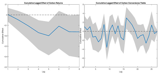
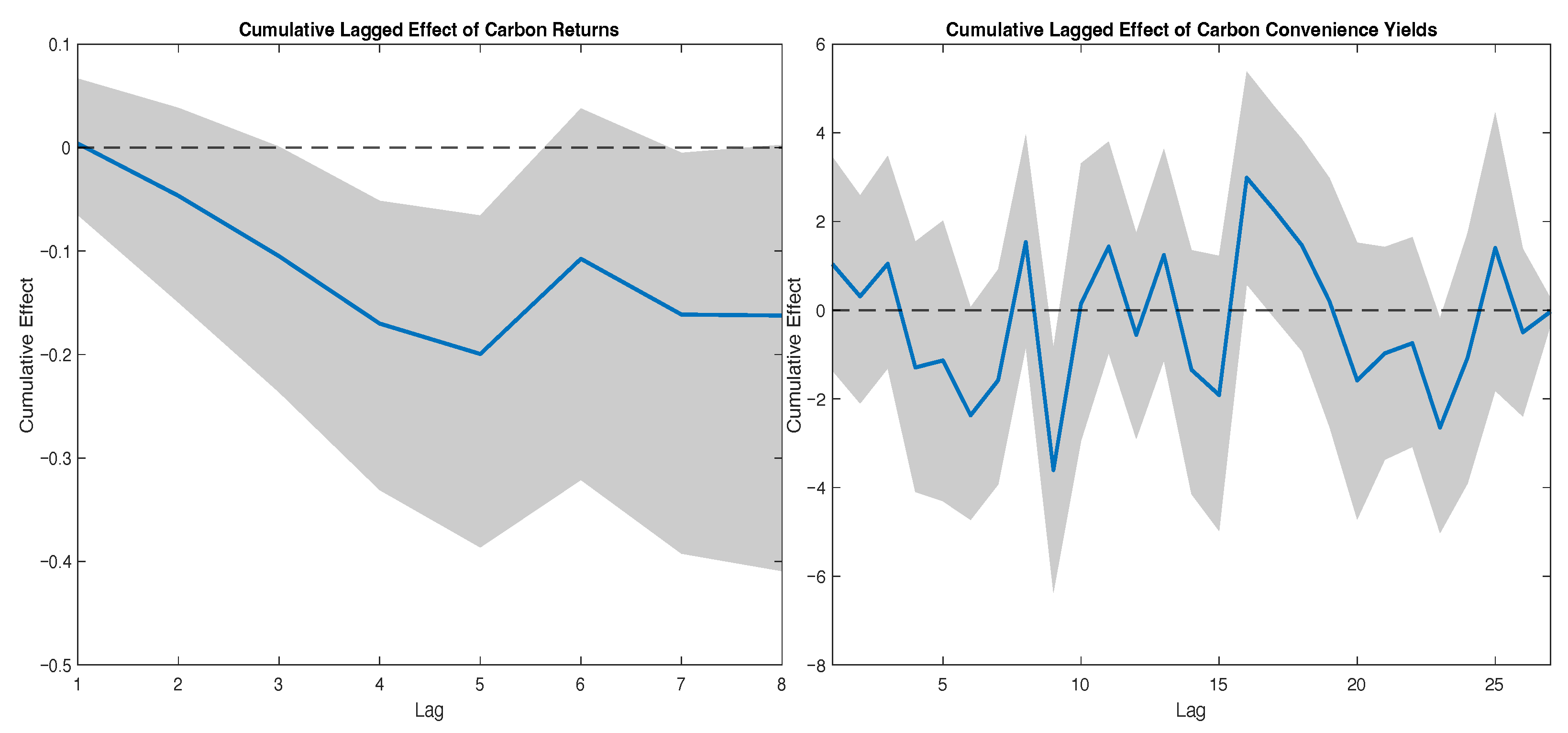
Figure 4 depicts the aggregated lagged effects implied by the U-$MIDAS$$(19,8,27)$ model, together with their 5–95% confidence intervals obtained via bootstrap procedures. The cumulative effect of carbon returns exhibits a clear negative pattern, becoming economically meaningful after the second lag and stabilizing at longer horizons. Although the confidence band includes zero, the monotonic accumulation suggests a persistent adverse impact that unfolds gradually over time rather than through short-lived fluctuations. This pattern is consistent with gradual information diffusion and trading frictions in the carbon market. In contrast, the cumulative effect of carbon convenience yields displays substantial time variation and alternates in sign across horizons. While the aggregated effect is statistically indistinguishable from zero, its magnitude is economically non-negligible, indicating that convenience yield shocks can generate sizable fluctuations in returns. The lack of statistical persistence suggests that the impact of convenience yields is highly state-dependent rather than stable over time, reflecting changing market conditions and regulatory environments. Overall, although convenience yields do not exert a statistically persistent cumulative effect, their dynamic and state-dependent responses embed valuable high-frequency information. This feature makes convenience yields an informative predictor for carbon returns, even in the absence of stable long-run effects.

Figure 4. The aggregated lagged effect of carbon returns and carbon convenience yields suggested by the $U\text{-}MIDAS(19,8,27)$ model.

To assess whether convenience yields contain incremental predictive information beyond established determinants, we conduct a comprehensive horse race against a wide set of benchmark models. These include $MIDAS$ specifications (including those based on energy prices, stock variables, and their combinations), alongside weekly traditional time-series models and nonlinear machine learning approaches. Specifically, the benchmark set includes U-$MIDAS(3,8,21)$-$oil$, $Step$-$MIDAS(3,8,37)$-$coal$, U-$MIDAS(4,8,6)$-$gas$, $Almon$-$MIDAS(3,8,3)$-$stock$, $MIDAS$ models combining energy and stock variables, as well as $ARDL$, $ARIMA(6,0,6)$, $GARCH(3,3)$, Random Forest ($RF$), RF with convenience yields ($RF$-y), $LSTM$, and $LSTM$ with convenience yields ($LSTM$-y) [43,44,50,51]. For the $MIDAS$ models, lag structures for energy and stock variables follow established practices in the literature [43], while return lags are determined by the results of this study. Forecast combination weights are assigned based on predictive accuracy measured by Mean Squared Error (MSE). For the traditional models, the $ARDL$ specification is configured to incorporate both the autocorrelation of carbon returns and the impact of convenience yields. Based on our findings, we set a maximum lag of 8 weeks for returns and a lag between 4 to 9 weeks for convenience yields. The parameters for the $ARIMA(6,0,6)$ and $GARCH(3,3)$ models are selected via the Akaike Information Criterion (AIC); both are applied to forecast returns using historical return data.

Table 4 reports the RMSE, MSE, and MAE for all competing models. Across all metrics, U-$MIDAS(19,8,27)$ achieves the best forecasting performance, outperforming not only energy- and stock-based $MIDAS$ models but also nonlinear machine learning benchmarks. This finding indicates that daily convenience yield information is more informative for forecasting weekly carbon returns than either daily energy/stock market data or weekly convenience yields. Importantly, augmenting the combined energy-stock $MIDAS$ model ($MIDAS$-$oil$ + $coal$ + $gas$ + $stock$) with carbon convenience yields further improves predictive accuracy, as evidenced by lower RMSE, MSE, and MAE of the $MIDAS$-y + $oil$ + $coal$ + $gas$ + $stock$ model. This confirms that carbon convenience yields contain incremental predictive information beyond that embedded in standard energy prices and stock market indicators. Rather than merely proxying for omitted covariates, convenience yields capture additional market-specific signals related to inventory conditions, compliance incentives, and expectations in the carbon market that are not fully spanned by conventional predictors.

Table 4. Performance comparisons between $U\text{-}MIDAS(19,8,27)$ and benchmark models.

Bechmark	RMSE	MSE	MAE	D-M Test
U-$MIDAS(19,8,27)$	0.060977	0.003718	0.047295	–
U-$MIDAS(3,8,21)$-$oil$	0.063292	0.004006	0.048818	−2.142831 **
$Step$-$MIDAS(3,8,37)$-$coal$	0.071014	0.005043	0.052362	−2.407062 **
U-$MIDAS(4,8,6)$-$gas$	0.065509	0.004291	0.050356	−2.276699 **
$Almon$-$MIDAS(3,8,3)$-$stock$	0.061207	0.003746	0.048048	−0.196127
$MIDAS$-$oil$ + $coal$ + $gas$ + $stock$	0.062486	0.003905	0.048773	−1.582437
$MIDAS$-y+$oil$ + $coal$ + $gas$ + $stock$	0.061915	0.003833	0.048237	−1.282431
$ARDL$	0.062856	0.003951	0.048700	−1.666834 *
$ARIMA(6,0,6)$	0.062821	0.003946	0.048666	−1.662214 *
$GARCH(3,3)$	0.062691	0.003930	0.048526	−1.494448
$RF$	0.063249	0.004000	0.049898	−1.611833
$RF$-y	0.062888	0.003955	0.049300	−1.463528
$LSTM$	0.062839	0.003949	0.048718	−1.665017 *
$LSTM$-y	0.062839	0.003949	0.048718	−1.665495 *

Note: This table displays performance comparisons between $U\text{-}MIDAS(19,8,27)$ and benchmark models. D-M test refers to the Diebold–Mariano test. * and **, represent significance at 10% and 5% level, respectively. The bold value represents the smallest value.

To formally assess whether the observed performance gains are statistically significant, we conduct Diebold–Mariano (D–M) tests comparing U-MIDAS(19,8,27) with each benchmark model. The results in Table 4 show that the predictive accuracy of U-MIDAS(19,8,27) is significantly superior to that of oil-, coal-, gas-based MIDAS models, ARDL, ARIMA, LSTM, and LSTM-y at conventional significance levels.

Taken together, the combined evidence from loss functions and predictive comparison tests confirms that the convenience-yield-based MIDAS model delivers statistically and economically meaningful improvements in forecasting carbon returns.

4.2. Probability Density Forecast for Carbon Returns

Building on the point forecasts of carbon returns obtained from the U-MIDAS(19,8,27) model, we further evaluate the predictive performance from a distributional perspective by constructing probability density forecasts. Following the procedure described in Section 2.3.2, we employ a non-parametric bootstrap approach to account for parameter uncertainty and model-implied forecast uncertainty [45,48]. Specifically, for each out-of-sample week, we generate 9999 bootstrap forecasts of carbon returns, from which the predictive densities are estimated using kernel density methods as described in Section 2.3.3. This approach avoids imposing parametric distributional assumptions and is well suited to the pronounced non-Gaussian features of carbon returns.

To formally assess the quality of the density forecasts, we rely on proper scoring rules, namely the log predictive score (LS) and the continuous ranked probability score (CRPS), which jointly evaluate sharpness and calibration. Table 5 reports the summary statistics of these two scores over the out-of-sample period. The average log score of 1.459 indicates that, on average, the realized carbon returns receive relatively high probability under the forecasted distributions, suggesting good local calibration around the realized outcomes. At the same time, the mean CRPS equals 0.033, which is small relative to the unconditional volatility of weekly carbon returns (with a standard deviation exceeding 6%, as shown in Table 1). This magnitude implies that the entire predictive distributions are, on average, close to the empirical realizations, not only at the center but across the full support.

Table 5. Summary statistics of log scores and continuous ranked probability score (%).

Variables	Mean	Std. Dev	Min	Max	Obs.
$LS$	1.459	0.712	−1.950	2.038	164
$CRPS$	0.033	0.029	0.014	0.245	164

Note: LS refers to the log score and CRPS refers to the continuous ranked probability score.

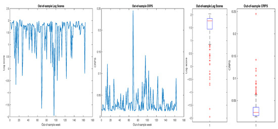
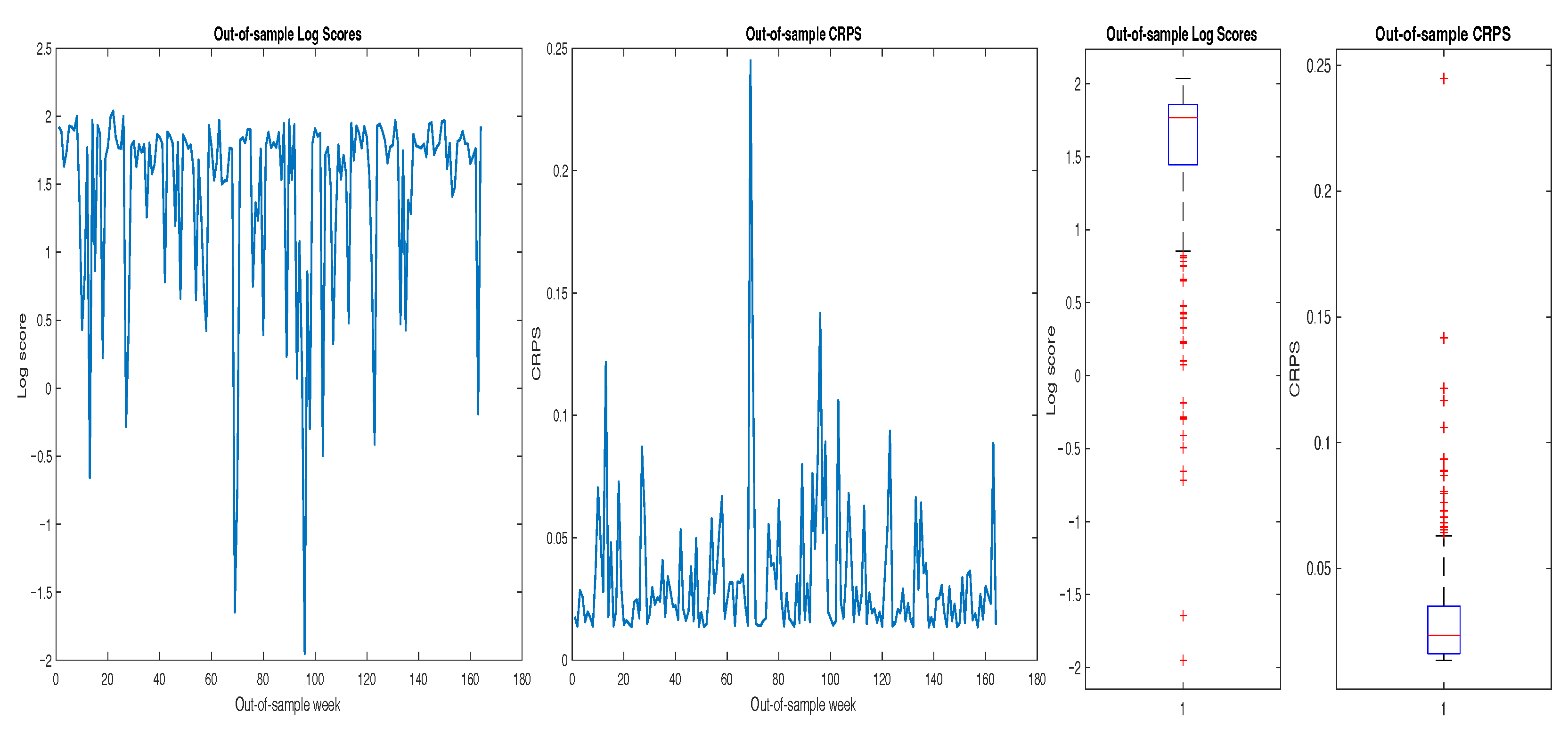
Figure 5 further illustrates the time variation in LS and CRPS across the out-of-sample weeks. While both scores exhibit occasional spikes—reflecting weeks with unusually large return realizations or abrupt market movements—the majority of observations cluster around stable and moderate values. Importantly, periods associated with lower log scores tend to coincide with higher CRPS values, indicating a coherent deterioration in density forecast performance during episodes of elevated uncertainty rather than isolated metric-specific anomalies. This consistency across scoring rules reinforces the reliability of the evaluation.

Figure 5. The variation of log scores (LS) and continuous ranked probability score (CRPS).

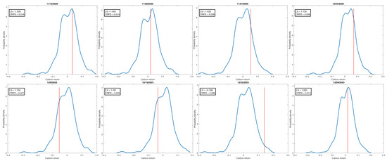
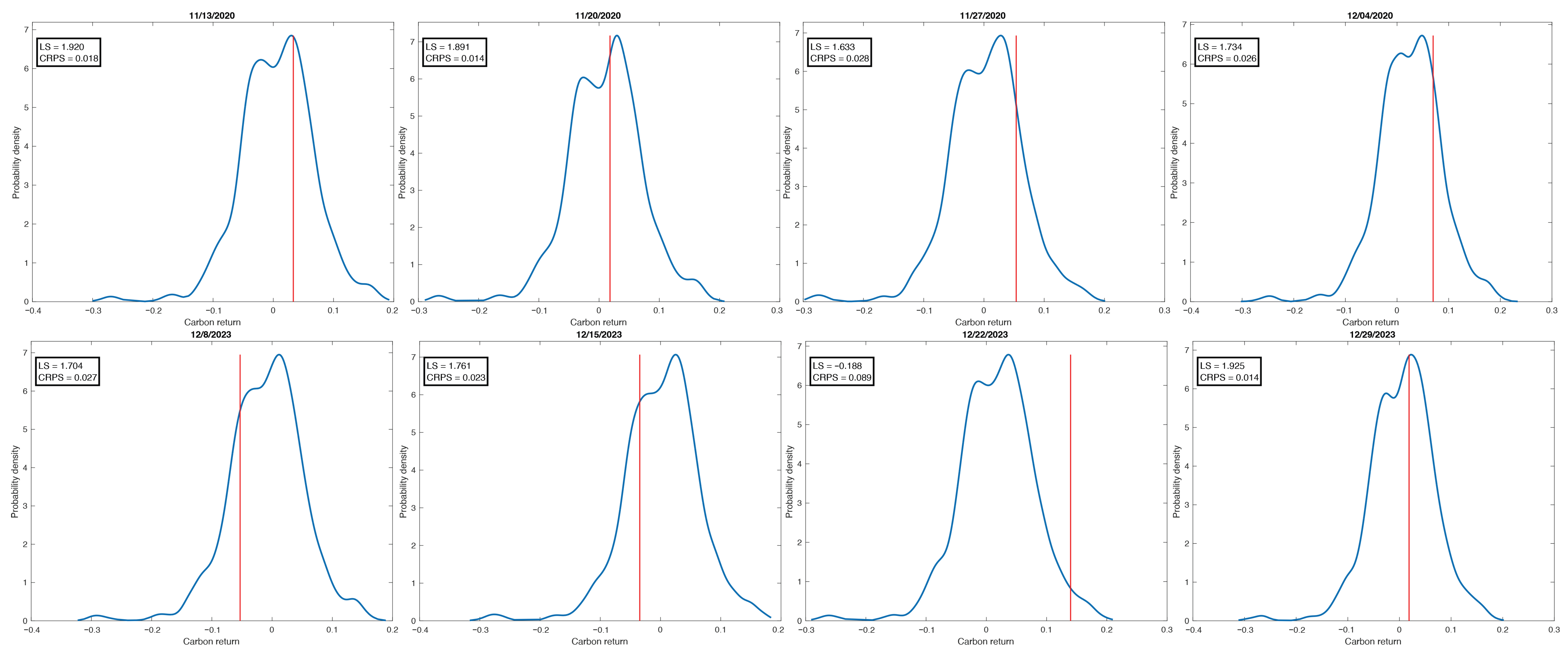
Figure 6 complements the scoring-rule-based assessment by visualizing the predictive densities for selected weeks at the beginning and end of the out-of-sample period. For each week, the realized carbon return is evaluated against the full forecast distribution rather than its modal value alone [52]. The reported LS and CRPS values within each panel confirm that weeks in which realized returns fall in regions of high predictive probability are associated with higher log scores and lower CRPS, whereas weeks with larger forecast errors are penalized accordingly. This alignment between visual evidence and formal scoring metrics suggests that the density forecasts are both well calibrated and appropriately sharp.

Figure 6. The probability density forecasts for carbon returns. Note: The vertical line represents the real carbon return. LS refers to the log score and CRPS refers to the continuous ranked probability score.

Overall, the joint evidence from proper scoring rules and density visualizations indicates that the proposed MIDAS-based framework, incorporating carbon convenience yields, delivers statistically and economically meaningful probability density forecasts for carbon returns. Rather than relying on visual proximity to modal density, the evaluation based on LS and CRPS provides a formal and robust confirmation of predictive distribution accuracy.

4.3. Robustness Checks

In this section, we conduct a series of robustness checks to examine whether our main findings are sensitive to alternative specifications, sample selections, and implementation choices in the bootstrap-based density forecasting framework. Specifically, we consider (i) alternative proxies for carbon convenience yields, (ii) subsample analysis to address potential structural changes in the EU ETS, and (iii) sensitivity analyses for the bootstrap and kernel density estimation procedures, including resampling schemes (block bootstrap), bandwidth selection, bootstrap size, and kernel choice.

A first concern relates to the construction of carbon convenience yields. As described in Section 2.1, the convenience yield is defined as the futures basis adjusted by the risk-free interest rate. One may therefore question whether the predictive content attributed to convenience yields merely reflects the role of interest rates. To address this concern, we follow the common practice in the commodity literature [30] and use the futures basis alone as an alternative proxy for interest-rate-adjusted convenience yields. The corresponding forecasting results are reported in Table 6. Given the robustness of findings across error metrics (RMSE, MSE, and MAE), we present only the RMSE results here. We find that the U-$MIDAS(23,8,23)$ model delivers the best predictive performance when the basis is used as the explanatory variable. Importantly, both the optimal lag structure and the resulting forecasting accuracy are highly comparable to those obtained under the baseline specification using carbon convenience yields. This evidence suggests that the predictive role of convenience yields is not driven solely by the inclusion of interest rates, but instead reflects information embedded in the futures term structure itself.

Table 6. The best MIDAS models under conditions with different steps ahead (h) for basis.

h	Model Specification	RMSE
5	$BetaNN\text{-}MIDAS(5,8,24)$	0.061393
6	$BetaNN\text{-}MIDAS(6,8,23)$	0.061376
7	$Almon\text{-}MIDAS(7,7,23)$	0.061355
8	$Almon\text{-}MIDAS(8,7,31)$	0.061347
9	$Almon\text{-}MIDAS(9,7,31)$	0.061332
10	$Almon\text{-}MIDAS(10,3,30)$	0.061310
11	$Almon\text{-}MIDAS(11,7,29)$	0.061189
12	$Almon\text{-}MIDAS(12,7,28)$	0.061238
13	$Almon\text{-}MIDAS(13,8,27)$	0.061212
14	$Almon\text{-}MIDAS(14,8,26)$	0.061185
15	$Almon\text{-}MIDAS(15,8,25)$	0.061183
16	$Step\text{-}MIDAS(16,8,28)$	0.061022
17	$Almon\text{-}MIDAS(17,8,23)$	0.061158
18	$U\text{-}MIDAS(18,8,28)$	0.061048
19	$U\text{-}MIDAS(19,8,27)$	0.060585
20	$U\text{-}MIDAS(20,8,26)$	0.060583
21	$U\text{-}MIDAS(21,8,25)$	0.060579
22	$U\text{-}MIDAS(22,8,24)$	0.060577
23	$U\text{-}MIDAS(23,8,23)$	0.060548
24	$U\text{-}MIDAS(24,8,22)$	0.060673
25	$U\text{-}MIDAS(25,8,21)$	0.060817

Note: This table displays the best MIDAS models under conditions with different h ranging from 5 to 20 and their corresponding prediction performance. h refers to the number of steps ahead. The model is specified as $Weigth\text{-}MIDAS(h,p,q)$, where $Weight$ refers to the polynomial weight, including $Beta$, $BetaNN$, $ExpAlmon$, $Almon$, $Step$ and $UMIDAS$. The term p refers to the lag order for carbon returns, and q refers to the lag order for carbon basis. The bold value represents the smallest RMSE under different conditions.

A second concern is that the empirical analysis focuses on a specific sample period, which may limit external validity in the presence of structural changes in the EU ETS, such as phase transitions, backloading measures, and the introduction of the Market Stability Reserve. To address this issue, we conduct a subsample analysis starting from 4 January 2013, which largely corresponds to Phase III of the EU ETS and encompasses major institutional reforms. Table 7 reports the optimal MIDAS specifications under different forecast steps ahead in this subsample. The results indicate that the $Step$-$MIDAS(19,8,24)$ model achieves the lowest RMSE, MSE, and MAE. Table 8 further compares this model with a wide range of benchmark models considered in Section 4.1. The Diebold–Mariano test results show that the convenience-yield-based MIDAS model continues to outperform most benchmarks at conventional significance levels, indicating the persistent predictive power of convenience yields. Moreover, Table 9 shows that the density forecasting performance, measured by log scores and CRPS, remains quantitatively similar to that obtained in the full sample. Together, these results suggest that our main conclusions are not driven by a particular regulatory phase or sample period.

Table 7. The best $MIDAS$ models under conditions with different steps ahead (h) for convenience yields in the subsamples since 2013.

h	Model Specification	RMSE	MSE	MAE
5	$BetaNN$-$MIDAS(5,7,24)$	0.061478	0.003780	0.047141
6	$BetaNN$-$MIDAS(6,8,23)$	0.061447	0.003776	0.047222
7	$BetaNN$-$MIDAS(7,7,22)$	0.061457	0.003777	0.047150
8	$BetaNN$-$MIDAS(8,8,21)$	0.061430	0.003774	0.047228
9	$BetaNN$-$MIDAS(9,8,20)$	0.061417	0.003772	0.047244
10	$BetaNN$-$MIDAS(10,6,19)$	0.061437	0.003775	0.047188
11	$BetaNN$-$MIDAS(11,8,18)$	0.061373	0.003767	0.047260
12	$BetaNN$-$MIDAS(12,8,17)$	0.061336	0.003762	0.047261
13	$BetaNN$-$MIDAS(13,8,19)$	0.061280	0.003755	0.047137
14	$BetaNN$-$MIDAS(14,8,19)$	0.061173	0.003742	0.046997
15	$BetaNN$-$MIDAS(15,7,18)$	0.061140	0.003738	0.046908
16	$Step$-$MIDAS(16,3,27)$	0.061009	0.003722	0.045625
17	U-$MIDAS(17,8,12)$	0.060761	0.003692	0.047253
18	$Beta$-$MIDAS(18,1,19)$	0.062861	0.003952	0.048628
19	$\mathit{S}\mathit{t}\mathit{e}\mathit{p}$-$\mathit{M}\mathit{I}\mathit{D}\mathit{A}\mathit{S}\mathbf{(}\mathbf{19}\mathbf{,}\mathbf{8}\mathbf{,}\mathbf{24}\mathbf{)}$	0.060531	0.003664	0.046304
20	U-$MIDAS(20,8,10)$	0.060717	0.003687	0.047353

Note: This table displays the best MIDAS models under conditions with different h ranging from 5 to 20 and their corresponding prediction performance. h refers to the number of steps ahead. The model is specified as $Weigth\text{-}MIDAS(h,p,q)$, where $Weight$ refers to the polynomial weight, including $Beta$, $BetaNN$, $ExpAlmon$, $Almon$, $Step$ and $UMIDAS$. The term p refers to the lag order for carbon returns, and q refers to the lag order for carbon convenience yields. The bold value represents the smallest RMSE under different conditions.

Table 8. Performance comparisons between Step-MIDAS(19,8,24) and benchmark models in the subsample since 2013.

Bechmark	RMSE	MSE	MAE	D-M Test
$Step$-$MIDAS(19,8,24)$	0.060531	0.003664	0.046304	–
U-$MIDAS(3,8,21)$-$oil$	0.064128	0.004112	0.048310	−2.025514 **
$Step$-$MIDAS(3,8,37)$-$coal$	0.078880	0.006222	0.058344	−3.106591 ***
U-$MIDAS(4,8,6)$-$gas$	0.071336	0.005089	0.054333	−3.190016 ***
$Almon$-$MIDAS(3,8,3)$-$stock$	0.061423	0.003773	0.047304	−0.739668
$MIDAS$-$oil$ + $coal$ + $gas$ + $stock$	0.062570	0.003915	0.048086	−1.662667 *
$MIDAS$-y+$oil$ + $coal$ + $gas$ + $stock$	0.061668	0.003803	0.047421	−1.227145
$ARDL$	0.063152	0.003988	0.049032	−1.896449 *
$ARIMA(6,0,6)$	0.062645	0.003924	0.048289	−1.738884 *
$GARCH(3,3)$	0.062669	0.003927	0.048508	−1.836611 *
$RF$	0.063700	0.004058	0.049553	−2.144668 **
$RF$-y	0.063552	0.004039	0.049068	−1.774468 *
$LSTM$	0.062499	0.003906	0.048335	−1.719998 *
$LSTM$-y	0.062622	0.003921	0.048436	−1.792479 *

Note: This table displays performance comparisons between $U\text{-}MIDAS(19,8,27)$ and benchmark models. D-M test refers to the Diebold–Mariano test. *, **, *** represent significance at 10%, 5%, and 1% level, respectively.

Table 9. Summary statistics of log scores and continuous ranked probability score in the subsample since 2013 (%).

Variables	Mean	Std. Dev	Min	Max	Obs.
$LS$	1.4694	0.6918	−1.3874	1.9995	164
$CRPS$	0.0329	0.0288	0.0131	0.2377	164

Note: LS refers to the log score and CRPS refers to the continuous ranked probability score.

A third set of robustness checks addresses concerns regarding the bootstrap and kernel density estimation procedures. In the baseline analysis, we apply an i.i.d. bootstrap to the model residuals. Given the presence of serial dependence and time-varying volatility in carbon returns, we additionally implement a moving block bootstrap to preserve local temporal dependence. Specifically, we adopt a block length of $L=8$, which is consistent with the empirical autocorrelation structure of carbon returns and closely approximates the conventional rule-of-thumb $L\approx T^{1/3}$, where T denotes the length of the in-sample period. The results under the block bootstrap are summarized in Panel A of Table 10. Both the mean log score and CRPS are nearly identical to those obtained under the i.i.d. bootstrap, indicating that the quality of the density forecasts is not sensitive to the resampling scheme. We further examine the sensitivity of the results to key implementation choices. Panel B considers an alternative bandwidth selection rule, using Silverman’s rule of thumb instead of the default data-driven optimal bandwidth employed in the baseline analysis. Panel C reduces the bootstrap size from 9999 to 1000 replications, and Panel D replaces the Gaussian kernel with the Epanechnikov kernel. Across all cases, the resulting log scores and CRPS remain remarkably stable in both magnitude and dispersion.

Table 10. Summary statistics of log scores and continuous ranked probability score under alternative bootstrap schemes (%).

Variables	Mean	Std. Dev	Min	Max	Obs.
Panel A: Block bootstrap with L = 8
$LS$	1.456	0.717	−2.217	1.985	164
$CRPS$	0.033	0.029	0.013	0.244	164
Panel B: Bandwidth selection
$LS$	1.459	0.712	−1.951	2.035	164
$CRPS$	0.033	0.029	0.014	0.245	164
Panel C: Bootstrap size (1000)
$LS$	1.448	0.693	−1.900	1.967	164
$CRPS$	0.033	0.029	0.013	0.245	164
Panel D: Kernel choice
$LS$	1.457	0.714	−1.933	2.029	164
$CRPS$	0.033	0.029	0.014	0.245	164

Note: LS refers to the log score and CRPS refers to the continuous ranked probability score.

Overall, these robustness checks indicate that our findings are not driven by specific modeling choices, resampling schemes, or tuning parameters. The predictive and density forecasting advantages associated with carbon convenience yields persist across alternative proxies, subsamples, and bootstrap implementations, lending strong support to the reliability of our empirical conclusions.

5. Conclusions

This paper studies the predictive role of carbon convenience yields for carbon returns and, more importantly, provides probability density forecasts for carbon returns within a unified forecasting framework. While the prediction of carbon prices and returns has attracted considerable attention from policymakers, investors, and researchers, the existing literature has largely focused on point forecasts and standard linear models. In contrast, formal density forecasting for carbon returns and the role of carbon convenience yields in this context remain relatively underexplored. At the same time, carbon returns are known to be influenced by a wide range of factors, including energy prices, financial market conditions, and macroeconomic variables. Whether carbon convenience yields contain incremental predictive information beyond these standard factors is therefore an open and economically relevant question.

To do so, we first examine the empirical properties of carbon convenience yields within the framework of the theory of storage. We then employ $MIDAS$ regressions to exploit the mixed-frequency nature of the data, linking daily carbon convenience yields to weekly carbon returns. In addition to point forecasts, we construct probability density forecasts for weekly carbon returns using a non-parametric bootstrap combined with kernel density estimation, allowing us to evaluate forecast uncertainty using proper scoring rules.

Using December futures contracts in the EU ETS from February 2008 to December 2023, we document several robust findings. First, the European carbon market has remained persistently contangoed since 2008, with carbon convenience yields turning predominantly negative after 2009. This pattern reflects the institutional features of the EU ETS, including allowance banking rules, compliance timing, and episodes of allowance surplus, which collectively reduce the benefits of physically holding allowances relative to futures positions. Second, shocks to carbon convenience yields affect carbon returns with economically meaningful dynamics: the response materializes with a delay of roughly hree weeks and persists for about four weeks thereafter. The estimated response paths highlight the role of convenience yields as a transmission channel from market tightness to returns.

From a forecasting perspective, our results show that $MIDAS$ models incorporating carbon convenience yields consistently outperform a broad set of benchmark models, including $ARDL$, $ARIMA$, $GARCH$, and $MIDAS$ models based on energy prices and stock market indicators, as well as machine learning approaches such as random forests and $LSTM$ models. Importantly, even when energy prices and stock market variables are included in the forecasting framework, carbon convenience yields retain incremental predictive content. This finding indicates that convenience yields do not merely proxy for standard predictors but capture additional information embedded in the carbon futures term structure. Beyond point forecasts, we formally evaluate the quality of density forecasts using proper scoring rules, including log scores and the continuous ranked probability score (CRPS). The results indicate that the proposed density forecasts are well calibrated and competitive across time, with realized returns typically occurring in high-probability regions of the predictive distributions. These conclusions are further supported by extensive robustness checks.

The empirical evidence in this paper has several implications. For policymakers, persistently negative convenience yields signal structural features of the carbon market—such as allowance surplus and intertemporal compliance incentives—that may weaken incentives to hold allowances. Probability density forecasts provide an additional tool for assessing not only expected returns but also the uncertainty surrounding future market outcomes, which is particularly relevant for evaluating policy interventions and market stability. For investors, the results highlight the value of carbon convenience yields as an informative predictor of returns and risks. Density forecasts offer a more comprehensive view of return distributions than point forecasts alone, facilitating risk management, portfolio allocation, and timing decisions in carbon markets.

There are still some limitations warranting further investigation. While this study focuses on December futures contracts due to their superior liquidity, extending the analysis to other maturities or to emerging carbon markets could further enhance external validity. Moreover, although $MIDAS$ models effectively capture mixed-frequency dynamics, alternative nonlinear or regime-switching frameworks may provide additional insights into the evolving structure of carbon markets, particularly in the presence of policy-induced regime shifts. Exploring these directions would further deepen our understanding of carbon asset pricing and forecasting under climate policy uncertainty.

References

- Nordhaus, W. Climate change: The ultimate challenge for economics. Am. Econ. Rev. 2019, 109, 1991–2014. [Google Scholar] [CrossRef] [Scilit]
- Zhu, B.; Ye, S.; Han, D.; Wang, P.; He, K.; Wei, Y.; Xie, R. A multiscale analysis for carbon price drivers. Energy Econ. 2019, 78, 202–216. [Google Scholar] [CrossRef] [Scilit]
- Sun, W.; Huang, C. A novel carbon price prediction model combines the secondary decomposition algorithm and the long short-term memory network. Energy 2020, 207, 118294. [Google Scholar] [CrossRef] [Scilit]
- Zhao, L.; Miao, J.; Qu, S.; Chen, X. A multi-factor integrated model for carbon price forecasting: Market interaction promoting carbon emission reduction. Sci. Total Environ. 2021, 796, 149110. [Google Scholar] [CrossRef] [Scilit] [PubMed]
- Zhang, W.; Wu, Z.; Zeng, X.; Zhu, C. An ensemble dynamic self-learning model for multiscale carbon price forecasting. Energy 2023, 263, 125820. [Google Scholar] [CrossRef] [Scilit]
- Madaleno, M.; Pinho, C. Risk premia in CO2 allowances: Spot and futures prices in the EEX market. Manag. Environ. Qual. Int. J. 2011, 22, 550–565. [Google Scholar] [CrossRef] [Scilit]
- Chang, K.; Wang, S.S.; Peng, K. Mean reversion of stochastic convenience yields for CO2 emissions allowances: Empirical evidence from the EU ETS. Span. Rev. Financ. Econ. 2013, 11, 39–45. [Google Scholar] [CrossRef] [Scilit]
- Chevallier, J. Carbon price drivers: An updated literature review. Int. J. Appl. Logist. (IJAL) 2013, 4, 1–7. [Google Scholar] [CrossRef] [Scilit]
- Creti, A.; Jouvet, P.A.; Mignon, V. Carbon price drivers: Phase I’ versus phase II equilibrium? Energy Econ. 2012, 34, 327–334. [Google Scholar] [CrossRef] [Scilit]
- Demiralay, S.; Gencer, H.G.; Bayraci, S. Carbon credit futures as an emerging asset: Hedging, diversification and downside risks. Energy Econ. 2022, 113, 106196. [Google Scholar] [CrossRef] [Scilit]
- Truck, S.; Weron, R. Convenience yields and risk premiums in the ¨ EU-ETS-Evidence from the kyoto commitment period. J. Futur. Mark. 2016, 36, 587–611. [Google Scholar] [CrossRef] [Scilit]
- Afonin, A.; Bredin, D.; Cuthbertson, K.; Muckley, C.; Nitzsche, D. Carbon portfolio management. Int. J. Financ. Econ. 2018, 23, 349–361. [Google Scholar] [CrossRef] [Scilit]
- Hintermann, B.; Peterson, S.; Rickels, W. Price and market behavior in phase II of the EU ETS: A review of the literature. In Review of Environmental Economics and Policy; Association of Environmental and Resource Economists: Washington, DC, USA, 2016. [Google Scholar]
- Azlen, M.; Gostlow, G.; Child, A. The carbon risk premium. J. Altern. Invest. 2022, 25, 33–64. [Google Scholar] [CrossRef] [Scilit]
- Huang, Y.; Dai, X.; Wang, Q.; Zhou, D. A hybrid model for carbon price forecasting using GARCH and long short-term memory network. Appl. Energy 2021, 285, 116485. [Google Scholar] [CrossRef] [Scilit]
- Lin, B.; Xu, B. A non-parametric analysis of the driving factors of China’s carbon prices. Energy Econ. 2021, 104, 105684. [Google Scholar] [CrossRef] [Scilit]
- Zhou, F.; Huang, Z.; Zhang, C. Carbon price forecasting based on CEEMDAN and LSTM. Appl. Energy 2022, 311, 118601. [Google Scholar] [CrossRef] [Scilit]
- Wang, Y.; Qin, L.; Wang, Q.; Chen, Y.; Yang, Q.; Xing, L.; Ba, S. A novel deep learning carbon price short-term prediction model with dualstage attention mechanism. Appl. Energy 2023, 347, 121380. [Google Scholar] [CrossRef] [Scilit]
- Chevallier, J. A model of carbon price interactions with macroeconomic and energy dynamics. Energy Econ. 2011, 33, 1295–1312. [Google Scholar] [CrossRef] [Scilit]
- Wen, F.; Zhao, H.; Zhao, L.; Yin, H. What drive carbon price dynamics in China? Int. Rev. Financ. Anal. 2022, 79, 101999. [Google Scholar] [CrossRef] [Scilit]
- Batten, J.A.; Maddox, G.E.; Young, M.R. Does weather, or energy prices, affect carbon prices? Energy Econ. 2021, 96, 105016. [Google Scholar] [CrossRef] [Scilit]
- Gong, X.; Li, M.; Guan, K.; Sun, C. Climate change attention and carbon futures return prediction. J. Futur. Mark. 2023, 43, 1261–1288. [Google Scholar] [CrossRef] [Scilit]
- Huang, Y.; He, Z. Carbon price forecasting with optimization prediction method based on unstructured combination. Sci. Total Environ. 2020, 725, 138350. [Google Scholar] [CrossRef] [Scilit] [PubMed]
- Li, J.; Liu, D. Carbon price forecasting based on secondary decomposition and feature screening. Energy 2023, 278, 127783. [Google Scholar] [CrossRef] [Scilit]
- Pindyck, R.S. The present value model of rational commodity pricing. Econ. J. 1993, 103, 511–530. [Google Scholar] [CrossRef] [Scilit]
- Daskalakis, G.; Psychoyios, D.; Markellos, R.N. Modeling CO2 emission allowance prices and derivatives: Evidence from the European trading scheme. J. Bank. Financ. 2009, 33, 1230–1241. [Google Scholar] [CrossRef] [Scilit]
- Palao, F.; Pardo, A. The inconvenience yield of carbon futures. Energy Econ. 2021, 101, 105461. [Google Scholar] [CrossRef] [Scilit]
- Almansour, A. Convenience yield in commodity price modeling: A regime switching approach. Energy Econ. 2016, 53, 238–247. [Google Scholar] [CrossRef] [Scilit]
- Keynes, J.M. Treatise on Money: Pure Theory of Money Vol. I; Kessinger Publishing: Whitefish, MT, USA, 1930. [Google Scholar]
- Han, M. Commodity momentum and reversal: Do they exist, and if so, why? J. Futur. Mark. 2023, 43, 1204–1237. [Google Scholar] [CrossRef] [Scilit]
- Brennan, M.J. The supply of storage. Am. Econ. Rev. 1958, 48, 50–72. [Google Scholar]
- Kaldor, N. Speculation and economic stability. Rev. Econ. Stud. 1939, 7, 1–27. [Google Scholar] [CrossRef] [Scilit]
- Working, H. The theory of price of storage. Am. Econ. Rev. 1949, 39, 1254–1262. [Google Scholar]
- Niu, X.; Wang, J.; Wei, D.; Zhang, L. A combined forecasting framework including point prediction and interval prediction for carbon emission trading prices. Renew. Energy 2022, 201, 46–59. [Google Scholar] [CrossRef] [Scilit]
- Manzan, S.; Zerom, D. A bootstrap-based non-parametric forecast density. Int. J. Forecast. 2008, 24, 535–550. [Google Scholar] [CrossRef] [Scilit]
- Cao, Y.; Zha, D.; Wang, Q.; Wen, L. Probabilistic carbon price prediction with quantile temporal convolutional network considering uncertain factors. J. Environ. Manag. 2023, 342, 118137. [Google Scholar] [CrossRef] [Scilit]
- Tian, C.; Hao, Y. Point and interval forecasting for carbon price based on an improved analysis-forecast system. Appl. Math. Model. 2020, 79, 126–144. [Google Scholar] [CrossRef] [Scilit]
- Zhu, M.; Xu, H.; Wang, M.; Tian, L. Carbon price interval prediction method based on probability density recurrence network and interval multi-layer perceptron. Phys. A Stat. Mech. Its Appl. 2024, 636, 129543. [Google Scholar] [CrossRef] [Scilit]
- Chen, B.; Gel, Y.R.; Balakrishna, N.; Abraham, B. Computationally efficient bootstrap prediction intervals for returns and volatilities in ARCH and GARCH processes. J. Forecast. 2011, 30, 51–71. [Google Scholar] [CrossRef] [Scilit]
- Ding, L.; Zhao, Z.; Han, M. Probability density forecasts for steam coal prices in China: The role of high-frequency factors. Energy 2021, 220, 119758. [Google Scholar] [CrossRef] [Scilit]
- Ding, L.; Zhao, Z.; Wang, L. Probability density forecasts for natural gas demand in China: Do mixed-frequency dynamic factors matter? Appl. Energy 2022, 312, 118756. [Google Scholar] [CrossRef] [Scilit]
- Ghysels, E.; Sinko, A.; Valkanov, R. MIDAS regressions: Further results and new directions. Econom. Rev. 2007, 26, 53–90. [Google Scholar] [CrossRef] [Scilit]
- Zhao, X.; Han, M.; Ding, L.; Kang, W. Usefulness of economic and energy data at different frequencies for carbon price forecasting in the EU ETS. Appl. Energy 2018, 216, 132–141. [Google Scholar] [CrossRef] [Scilit]
- Han, M.; Ding, L.; Zhao, X.; Kang, W. Forecasting carbon prices in the Shenzhen market, China: The role of mixed-frequency factors. Energy 2019, 171, 69–76. [Google Scholar] [CrossRef] [Scilit]
- Truc´ıos, C.; Hotta, L.K. Bootstrap prediction in univariate volatility models with leverage effect. Math. Comput. Simul. 2016, 120, 91–103. [Google Scholar] [CrossRef] [Scilit]
- Chevallier, J. Modelling the convenience yield in carbon prices using daily and realized measures. Int. Rev. Appl. Financ. Issues Econ. 2009, 1, 56–73. [Google Scholar]
- Prokopczuk, M.; Symeonidis, L.; Simen, C.W.; Wichmann, R. Convenience yield risk. Energy Econ. 2023, 120, 106536. [Google Scholar] [CrossRef] [Scilit]
- Tian, W.; Song, J.; Li, Z.; de Wilde, P. Bootstrap techniques for sensitivity analysis and model selection in building thermal performance analysis. Appl. Energy 2014, 135, 320–328. [Google Scholar] [CrossRef] [Scilit]
- Boons, M.; Prado, M.P. Basis-momentum. J. Financ. 2019, 74, 239–279. [Google Scholar] [CrossRef] [Scilit]
- Zhao, X.; Li, H.; Ding, L.; Wang, W.; Xue, Y. Forecasting direct economic losses of marine disasters in china based on a novel combined model. Int. Disaster Risk Reduct. 2020, 51, 101921. [Google Scholar] [CrossRef] [Scilit]
- Zhao, X.; Li, H.; Ding, L.; Liu, M. Research and application of a hybrid system based on interpolation for forecasting direct economic losses of marine disasters. Int. J. Disaster Risk Reduct. 2019, 37, 101121. [Google Scholar] [CrossRef] [Scilit]
- Lei, H.; Xue, M.; Liu, H. Probability distribution forecasting of carbon allowance prices: A hybrid model considering multiple influencing factors. Energy Econ. 2022, 113, 106189. [Google Scholar] [CrossRef] [Scilit]
Disclaimer/Publisher’s Note: The statements, opinions and data contained in all publications are solely those of the individual author(s) and contributor(s) and not of MDPI and/or the editor(s). MDPI and/or the editor(s) disclaim responsibility for any injury to people or property resulting from any ideas, methods, instructions or products referred to in the content. |
© 2026 by the authors. Licensee MDPI, Basel, Switzerland. This article is an open access article distributed under the terms and conditions of the Creative Commons Attribution (CC BY) license.