On a Pseudo-Orthogonality Condition Related to Cyclic Self-Mappings in Metric Spaces and Some of Their Relevant Properties

Abstract

This paper relies on orthogonal metric spaces related to cyclic self-mappings and some of their relevant properties. The involved binary relation is not symmetric, and then the term pseudo-orthogonality will be used for the relation used in the article to address the established results on cyclic self-mappings. Firstly, some orthogonal binary relations are given through examples to fix some ideas to be followed in the main body of the article. It is seen that the orthogonal elements of the orthogonal sets are not necessarily singletons. Secondly, “ad hoc” specific orthogonality binary relations are also described through examples related to the investigation of stability and controllability problems in dynamic systems. The main objective of this paper is to investigate the properties of cyclic single-valued self-mappings on the union of any finite number $p\ge 2$ of nonempty closed subsets of a metric space in a cyclic disposal under an “ad hoc” defined pseudo-orthogonality condition. Such a condition is defined on certain subsequences, referred to as pseudo-orthogonal sequences, rather than on the whole generated sequences under the self-mapping. It basically consists of a cyclic, in general iteration-dependent, contractive condition just for such subsequences which, on the other hand, are not forced as a constraint to be fulfilled by the whole sequences. Furthermore, the whole sequences in which those sequences are contained are allowed to be locally non-contractive or even locally expansive. The boundedness and the convergence properties of distances between pseudo-orthogonal subsequences and sequences are investigated under the condition that one of the subsets has a unique best proximity point to its adjacent subset in the cyclic disposal to which the pseudo-orthogonal subsequences converge. The pseudo-orthogonal metric subspace of the given metric space is proved to be complete although the whole metric space is not assumed to be complete. The pseudo-orthogonal element is seen to be a set of best proximity points, one per subset of the cyclic disposal, although it is not required for all the best proximity sets to be singletons. It is proved that the pseudo-orthogonal subsequences converge to a limit cycle, consisting of a best proximity point per subset of the cyclic disposal, which is also the pseudo-orthogonal element. The whole sequences are also proved to be bounded and the distances between their elements in adjacent subsets are also proved to converge to the distance between adjacent subsets. In the event that the metric space is a uniformly convex Banach space, it suffices that one of the subsets of the cyclic disposal be boundedly compact with its best proximity set being a singleton. In this case, the pseudo-orthogonal sequences converge to their best proximity set to their adjacent subset provided that such a best proximity set is a singleton.

1. Introduction

The properties of the so-called contractive cyclic self-mappings have been exhaustively studied in metric and, in particular, in Banach spaces [1,2,3,4,5,6,7,8]. Also, the so-called cyclic ${\varphi }_A$-contractions, the cyclic mappings in multiplicative metric spaces as well as the cyclic mappings on partially ordered and on orbitally complete metric spaces have been investigated in [9,10,11,12], and some references therein, for the cases of b-metric and b-metric-like spaces and also in the context of Hardy–Rogers contractions [13]. On the other hand, some proximity properties have been reported in [14] for Busemann convex metric spaces. In [15,16,17], BSS cyclic mappings, S-cyclic mappings and Kannan S-coupled cyclic mappings have been investigated together with their boundedness and convergence associated properties. The important concepts of approximative compactness and bounded compactness, which lead to ensure the non-emptiness of the sets of best proximity points in subsets of metric spaces, have been addressed in [1,18,19].

It is also well-known that the framework of cyclic contractions might be appropriate for the investigation of the stabilization of dynamic systems under switching actions concerning different model parameterizations or under eventual different modes of operation, that is, under different configurations [20,21,22,23,24]. The main reason for such a usefulness relies on the fact that each one of the individual system’s configurations can be embedded for analysis into one particular subset of the cyclic disposal [25,26,27,28].

On the other hand, it turns out that the so-called enriched contractions are characterized by some extra parameters apart from the usual contractive constants so that the properties of interest of contractions such as boundedness and convergence of distances or existence and uniqueness of fixed points and convergence properties of sequences to them are commonly achievable under less stringent conditions. The available background research on those classes of contractions is exhaustive. In particular, in [29] extensions of the Banach contraction mapping from metric and Banach spaces are developed. In [30], the uniqueness of fixed points and their allocation are approximated via a Krasnoselskij iterative scheme. Also, Chatterjea-type enriched contractions with their associate fixed point properties were investigated in [31] and some of the references therein. On the other hand, enriched Ćirić–Reich–Rus contractions and quasi-contractions in Banach spaces and in convex metric spaces were addressed in [32,33]. Also, an enriched cyclic Kannan-type contraction was proposed in [34] on a Banach space and the existence and uniqueness of a fixed point was proven. In [35], a new approach of enriched contractions and enriched non-expansive mappings was given, which permits in a novel way the use of Mann iteration related to Kasnoselskij-type iterations. Also, fixed point results concerned enriched Kannan mappings in CAT(0) spaces and enriched rational-type contractions in both quasi-Banach spaces and n-generalized convex b-metric spaces were investigated in [36,37]. In [38], a Krasnoselskij-type iteration-based convergence result for cyclic contractions was proved, while in [39] generalized cyclic contractions were defined in Banach spaces and a concerned fixed point theorem was stated. Also, non-expansive mappings in ordered CAT(0) spaces have been studied in [40] for approximation of fixed points and, in [41], certain iterative schemes in Banach spaces were investigated for enriched contractive and asymptotically non-expansive maps. More recently, enriched cyclic contractive self-mappings in metric spaces and in uniformly convex Banach spaces have been proposed and investigated in [42] for cyclical disposals, conformed by any number of two or more subsets, concerning the associated boundedness of sequences and their convergence properties to the best proximity points.

The current paper objective and content are supported by an idea which has been used in several works on fixed point theory and applications. Such an idea has been the introduction of binary orthogonality relations to first select some sequences (referred to as orthogonal sequences or, simply, as $O$-sequences) of the whole sequences at hand which verify the particular defined orthogonal relation together with the contractive conditions assumed on the metric (or Banach) space. Such sequences might be, in general, subsequences of the whole sequences of the metric space which are generated by a contractive self-mapping. The metric space $\left(X,d\right)$ together with the binary orthogonal relation $\perp$ becomes a so-called orthogonal metric space $\left(X,d,\perp \right)$, a metric subspace of $\left(X,d\right)$ [43,44], whose boundedness and convergence properties are, in principle, concerned with the orthogonal sequences while some of those properties are sometimes extendable to wider sequences of the metric space which contain those orthogonal sequences. It has been seen that the completeness of the orthogonal metric space $\left(X,d,\perp \right)$ does not necessarily imply that of the metric space $\left(X,d\right)$ [43,44].

In that formal context, it can be pointed out that the Banach fixed point theorem has been extended to orthogonal metric spaces in [44]. Fixed point theorems have been formulated in [45] for generalized orthogonal contractions. Also, extensions of F-weak contractions have been given in [46] for orthogonal weak contractions while Wardowski-type cyclic F-contractive mappings in orthogonal metric spaces and related proximity point results have been studied in [47]. On the other hand, multivalued F-contractions of rational type have been investigated in [48] on an orthogonal metric space while p-contractions have been extended to orthogonal metric spaces in [49].

The rest of the paper is organized as follows. Section 2 gives some preliminary basic definitions concerned with orthogonal relations together with six worked examples and some elementary results. Some of the examples rely on Hilbert spaces of square-integrable functions [50,51,52,53], on those concerned with the scalar product of real vectors (whose “orthogonality” binary relation coincides with the typical orthogonality of vectors in a geometric sense) or with the ordering relations on sets of integer numbers which have either a unique maximum number or several maximal ones. These two situations are key to illustrating in a simple manner if the orthogonal element is unique or not. In Section 3, some pseudo-orthogonality relations related to stability and controllability of dynamic systems are examined through seven “ad hoc” worked examples. Those examples are concerned with the properties of stability and controllability of continuous-time and discrete-time dynamic systems. It is pertinent to point out that, although the usual orthogonal relations are symmetric, there are also relevant non-symmetric relations available in the background literature, which have been referred to as orthogonal relations like, for instance, the celebrated Birkhoff–James orthogonality in general normed spaces. See, for instance [54] and several references therein. There are also (non-symmetric) orthogonal relations, sometimes referred to as bi-orthogonal, in quantum mechanics and in functional analysis. Those non-symmetric relations keep the essential properties of the orthogonal ones. Since the proposed relation is non-symmetric, as pointed out by one of the reviewers, we call it a pseudo-orthogonality relation. Such a pseudo-orthogonality condition is formulated to select some subsequences of the whole sequences for which the cyclic contraction constraint holds, and those subsequences are pseudo-orthogonal ($PO$)-sequences of the resulting pseudo-orthogonal metric space. The pseudo-orthogonality relations in the stability context are defined concerning convergence to a zero equilibrium state, which is the orthogonal element. In the controllability context, such sequences have a finite number of elements since the controllability property is related, as usual, to reach any prescribed state value along a finite time interval. It is seen that the concept of $PO$-sets, that is, the subsets of elements of the pseudo-orthogonal space which are pseudo-orthogonal to all the elements of such a space, and that of $PO$-sequences, together with their pseudo-orthogonality preservation, might also be useful in the stability, stabilizability, and controllability contextual analysis of dynamic systems. It can be pointed out that these concepts are very relevant in the fields of differential equations, differential systems of equations, and control theory [50,51,52,53]. Section 4 is devoted to single-valued cyclic self-mapping in metric spaces acting on a set of a finite number of two or more nonempty closed subsets of the metric space. The self-mappings are not necessarily contractive in each iteration being performed to generate the relevant sequences while they can be locally non-contractive or even locally expansive. The main properties of boundedness and convergence of the distances as well as those of boundedness, convergence, cauchyness, and pseudo-orthogonality preserving properties are firstly derived for such $PO$-sequences under the assumption that one of the subsets of the cyclic disposal has a single best proximity set to its adjacent subset, that is, the corresponding best proximity set is a singleton. Also, some of the properties of convergence and boundedness of distances and sequences are proved to be transmitted from the pseudo-orthogonal sequences to the whole sequences in which they are contained as subsequences. Some illustrative examples are also discussed in that section. Section 5 describes and discusses some further numerical worked examples and, finally, conclusions end the paper.

2. Preliminary Orthogonality Definitions, Assertions and Examples

The following notation is used in the following:

$${\mathit{Z}}_{0+}={\mathit{Z}}_{+}\cup \left\{0\right\}; {\mathit{Z}}_{+}=\left\{z\in \mathit{Z}\hspace{0.33em}:z>0\right\}; {\mathit{Z}}_{0-}={\mathit{Z}}_{-}\cup \left\{0\right\}; {\mathit{Z}}_{-}=\left\{z\in \mathit{Z}\hspace{0.33em}:z<0\right\};$$

$${\mathit{R}}_{0+}={\mathit{R}}_{+}\cup \left\{0\right\}; {\mathit{R}}_{+}=\left\{z\in \mathit{R}\hspace{0.33em}:z>0\right\}; {\mathit{R}}_{0-}={\mathit{R}}_{-}\cup \left\{0\right\}; {\mathit{R}}_{-}=\left\{z\in \mathit{R}\hspace{0.33em}:z<0\right\}$$

• $\mathit{Z},\mathit{R}\hspace{0.33em}\mathrm{and}\hspace{0.33em}\mathbf{C}$ are, respectively, the sets of integer, real and complex numbers;
• $\bar{n}=\left\{\mathrm{1,2},\dots ,n\right\}$;
• $I_d$ is the identity matrix of order $d$.

Superscripts $n$ in the above sets mean that all the components of $n$-tuples belonging to them are in the corresponding scalar counterpart. For example, $x=\left(x_i\right)\in {\mathit{R}}_{+}^n\iff x_i\in {\mathit{R}}_{+};\forall i\in \bar{n}$. The same notation is extended to matrices. For instance, $A=\left(A_{ij}\right)\in {\mathit{R}}_{+}^{n\times n}\iff A_{ij}\in {\mathit{R}}_{+};\forall i,j\in \bar{n}$; $clX$ is the closure of the set $X$. The following two definitions, borrowed from [44], are needed for the subsequent study:

Definition 1. 

Let a set $X\ne \varnothing$ be endowed with a binary relation $\perp$ such that $\exists z\in X$ for which $\left(\left[z\perp x;\forall x\in X\right]\vee \left[x\perp z\right];\forall x\in X\right)$. Then, $\left(X,\perp \right)$ is said to be an orthogonal set (in short, an $O$-set) and $z$ is called an orthogonal element.

Definition 2. 

If $\left(X,\perp \right)$ is an $O$-set then $x\hspace{0.33em},\hspace{0.33em}y\in X$ are orthogonally related (or, simply, $x\hspace{0.33em},\hspace{0.33em}y\in X$ are orthogonal) if $x\perp y$.

It turns out that, if $\left(X,\perp \right)$ is an $O$-set and $z\in X$ is an orthogonal element, then $x\perp z$ and $z\perp z$.

It can be pointed out that the fact that the orthogonality concept extends beyond a direct geometric interpretation is common to several different research fields. For instance, in [55], a conditional dependence between regression residuals may be reduced to an unconditional one between residuals that are orthogonal in a certain sense. Also, an interpretation of orthogonality is figured out in [56] on invertible matrices. On the other hand, trigonometric quadrature rules [57] are related to orthogonality when using orthogonal trigonometric polynomials, and the orthogonality of Chebyshev polynomials is very relevant for analysis in filtering and signal processing [58]. The HALTRAV design, see for instance [59], can be considered orthogonal to its hardware design in the sense that it is decoupled from physical simulation and the verification stage is separated from implementation.

Three simple illustrative examples follow below:

Example 1. 

Define $X=\left[-a\hspace{0.33em},\hspace{0.33em}a\right]$ for some $a\in {\mathit{R}}_{+}$ and, for any $x,y\in X$, define the orthogonal relation $x\perp y$ if $x.y\le 0$. Then, any elements with different sign, or such that at least one of them is zero, are orthogonal. The element $z=0$ is orthogonal to any $x\in X$ and it is the unique orthogonal element to any $x\in X$. It turns out that $\left(X,\perp \right)$ is an $O$-set.

Example 2. 

Define $X=\left[-a\hspace{0.33em},\hspace{0.33em}0\right)\cup \left(0,a\right]$ for some $a\in {\mathit{R}}_{+}$ and, for any $x,y\in X$, define the orthogonal relation $x\perp y$ if $x.y<0$, that is, if $\mathit{sgn}\left(x\right)=-\mathit{sgn}\left(y\right)$. It does not exist any orthogonal element so that $\left(X,\perp \right)$ is not an $O$-set. If the orthogonal relation is redefined by $x\perp y$ if $x.y\le 0$, the conclusion is identical so that $\left(X,\perp \right)$ is not an $O$-set either.

Example 3. 

Let $X={\mathit{R}}^n$ for any $n\ge 1$ and the orthogonality relation is defined by $x\perp y$ if $x^T.y=y^T.x=0$, where the superscript $“T”$ stands for transposition. Then $0\in {\mathit{R}}^n$ is the unique orthogonal element and $\left(X,\perp \right)$ is an $O$-set. This binary relation is the well-known orthogonality relation of the scalar product of real vectors of dimension $n$. Then, any elements with different sign, or such that at least one of them is zero, are orthogonal. The element $z=0$ is orthogonal to any $x\in X$ and it is the unique orthogonal element to any $x\in X$. It turns out that $\left(X,\perp \right)$ is an $O$-set.

Note that the orthogonal element might be non-unique, as pointed out in [44]. For instance, consider the two subsequent examples:

Example 4. 

Define the $O$-set $\left(X,\perp \right)$ by $X=\left\{\mathrm{1,2},\mathrm{3,4},-4\right\}$ and define $x\perp y$ if $\left|x\right|\le \left|y\right|$ for any given $x,y\in X$. Then, $1\perp 2$, $1\perp 3$, $1\perp 4$, $1\perp \left(-4\right)$, $2\perp 3$, $2\perp 4$, $2\perp \left(-4\right)$, $3\perp 4$, $3\perp \left(-4\right)$, $4\perp \left(-4\right)$, $\left(-4\right)\perp 4$ and $x\perp x$; $\forall x\in X$ and $\left(-4\right)$ and $4$ are two distinct orthogonal elements since the defined orthogonal relation, which is also an order relation, has two maximal elements (which are the orthogonal elements), then it has not a maximum. On the other hand, it turns out that if now $X=\left\{\mathrm{1,2},\mathrm{3,4}\right\}$ (respectively, if $X=\left\{\mathrm{1,2},3,-4\right\}$) then $4$ (respectively, $-4$) is the unique orthogonal element of the $O$-set $\left(X,\perp \right)$.

The above example concludes that, if $\left(X,\perp \right)$ is an $O$-set, then it exists an orthogonal subset $Z\left(\ne \varnothing \right)\subset X$ which can have a cardinality greater than unity. In this case, the orthogonal relation of Definition 1 becomes $\exists Z\left(\ne \varnothing \right)\subset X:\left(\left[z\perp x;\forall x\in X\right]\vee \left[x\perp z\right];\forall x\in X,\forall z\in Z\right)$.

We can denote, in short, $x\perp Z$; $\forall x\in X$ to express that any $x$ in $X$ is orthogonal to all the elements of $Z$, that is $x\perp z$; $\forall x\in X$, $\forall z\in Z$.

Example 5. 

Let $X_a$ be the Hilbert space of square-integrable real $n$-vector functions $f\in L_2^n\left(\left[0\hspace{0.33em},\hspace{0.33em}a\right]\hspace{0.33em};{\mathit{R}}^n\right)$ defined in $\left[0\hspace{0.33em},\hspace{0.33em}a\right]\subseteq {\mathit{R}}_{0+}$ for a given $a\in {\mathit{R}}_{+}$ endowed with the inner product $<f,g>={\int }_0^a{f}^T\left(t\right)g\left(t\right)dt$; $\forall f,g\in X_a$ which induces the seminorm $‖f‖=<f,f{>}^{1/2}={\left({\int }_0^a{f}^T\left(t\right)f\left(t\right)dt\right)}^{1/2}$; $\forall f\in X_a$, [50,51,53]. Then, $f\perp g$ if $<f,g>=0$. It turns out that $\left(X_a,\perp \right)$ is an $O$-set with orthogonal element $f_z\left(=0\right)\in X_a$ which is non-unique since the set $U_{fz}\subset X_a$ of bounded functions in $X_a$ of support of zero measure is an orthogonal set-element consisting of infinity many elements since $<f,f_z>=0$; $\forall f_z\in U_{fz}$; $\forall f\in X_a$.

If piecewise continuity is also requested in the definition o $X_a$, that is, $X_a$ is redefined by $X_a=\left\{f\in \left(P{C}^n\left(\left[0\hspace{0.33em},\hspace{0.33em}a\right]\hspace{0.33em};{\mathit{R}}^n\right)\cap L_2^n\left(\left[0\hspace{0.33em},\hspace{0.33em}a\right]\hspace{0.33em};{\mathit{R}}^n\right)\right)\right\}$ then $f_z\left(=0\right)\in X_a$ is the unique orthogonal element in this case.

The following definitions combine orthogonal relations with the framework of metric spaces invoking extended orthogonality-related concepts in metric spaces by combining both structures:

Definition 3. ([44]).

If $\left(X,\perp \right)$ is an $O$-set and $\left(X,d\right)$ is a metric space then:

3.1. 

The triple $\left(X,\perp ,d\right)$ is said to be an orthogonal metric space (in short, an $OMS$), a metric subspace of $\left(X,d\right)$.

3.2. 

If $\left(X,\perp ,d\right)$ is an $OMS$ then ${\left\{x_n\right\}}_{n\in {\mathit{Z}}_0}\subset X$ is said to be an orthogonal sequence (in short, an $O$-sequence) if $\left(\left[x_n\perp x_{n+1};\hspace{0.33em}\forall n\in {\mathit{Z}}_{0+}\right]\vee \left[x_{n+1}\perp x_n;\hspace{0.33em}\forall n\in {\mathit{Z}}_{0+}\right]\right)$. Two consecutive members $x_n$ and $x_{n+1}$ of the sequence ${\left\{x_n\right\}}_{n\in {\mathit{Z}}_0}\subset X$ are (pair-wise) orthogonal if $\left(\left[x_n\perp x_{n+1}\right]\vee \left[x_{n+1}\perp x_n\right]\right)$.

3.3. 

If $\left(X,\perp ,d\right)$ is an $OMS$ then the $O$-sequence ${\left\{x_n\right\}}_{n\in {\mathit{Z}}_0}\subset X$ is convergent if ${\left\{x_n\right\}}_{n\in {\mathit{Z}}_0}\to z\left(\in clX\right)$. Then, it is bounded as well.

3.4. 

If $\left(X,\perp ,d\right)$ is an $OMS$ then it is said to be orthogonally complete (in brief, $O-complete$) if each Cauchy $O$-sequence ${\left\{x_n\right\}}_{n\in {\mathit{Z}}_0}\subset X$ is convergent in $X$.

3.5. 

If $\left(X,\perp ,d\right)$ is an $OMS$ then $f:X\to X$ is orthogonally continuous (in brief, $\perp -$continuous) in $x\in X$ if $f\left(x_n\right)\to f\left(x\right)$ as $n\to \infty$ for each $O$-sequence ${\left\{x_n\right\}}_{n\in {\mathit{Z}}_0}\left(\subset X\right)\to x\left(\in X\right)$; and $f:X\to X$ is $\perp -$continuous in $X$ if it is $\perp -$continuous for all $x\in X$.

3.6. 

If $\left(X,\perp \right)$ is an $O$-set then $f:X\to X$ is orthogonally preserving (in short, $\perp -$preserving) if $\left[\left(x\perp y\right)\Rightarrow \left(f\left(x\right)\perp f\left(y\right)\right)\right];\forall x,y\in X$; and it is weakly orthogonally preserving (or weakly $\perp -$preserving) if $\left(x\perp y\right)\Rightarrow \left[\left(\left(f\left(x\right)\perp f\left(y\right)\right)\vee \left(f\left(y\right)\perp f\left(x\right)\right)\right)\right];\forall x,y\in X$. If the above properties hold for a concrete pair $\left(x,y\right)$ in $X\times X$, then the property is termed as $\perp -$preserving in $\left(x,y\right)$ (respectively, weakly $\perp -$preserving in $\left(x,y\right)$).

It turns out that, if $f:X\to X$ is $\perp -$preserving then it is also weakly $\perp -$preserving, $\perp -$preserving in any $\left(x,y\right)\in X\times X$, and weakly $\perp -$preserving, in any $\left(x,y\right)\in X\times X$.

Assertion 1. 

Any $O$-set has at least an orthogonal sequence.

Proof. 

If $\left(X,\perp \right)$ is an $O$-set, it has an orthogonal element $z\in X$. Then, the constant sequence ${\left\{x_n\right\}}_{n=0}^{\infty }\subset X$, defined by $x_n=z$; $\forall n\in {\mathit{Z}}_{0+}$ is an $O$-sequence. □

Assertion 2. 

If $\left(X,\perp ,d\right)$ has the property $\left(\left[x_n\perp x_{n+1};\hspace{0.33em}\forall n\in {\mathit{Z}}_{0+}\right]⥂\wedge \left[x_{n+1}\perp x_n;\hspace{0.33em}\forall n\in {\mathit{Z}}_{0+}\right]\right)$ then it is a $OMS$ so that $\left(\left[x_n\perp x_{n+1};\hspace{0.33em}\forall n\in {\mathit{Z}}_{0+}\right]\vee \left[x_{n+1}\perp x_n;\hspace{0.33em}\forall n\in {\mathit{Z}}_{0+}\right]\right)$.

Proof. 

From Definition 3(3.2), ${\left\{x_n\right\}}_{n\in {\mathit{Z}}_0}\subset X$ is an $O$-sequence if $\left(\left[x_n\perp x_{n+1};\hspace{0.33em}\forall n\in {\mathit{Z}}_{0+}\right]⥂\vee \left[x_{n+1}\perp x_n;\hspace{0.33em}\forall n\in {\mathit{Z}}_{0+}\right]\right)$. Now, note that the disjunction logic proposition ($\vee ,say“or”$) of two premises is true if its conjunction ($\wedge ,say“and”$) is true. Thus,$\left(\left[x_n\perp x_{n+1};\hspace{0.33em}\forall n\in {\mathit{Z}}_{0+}\right]\wedge \left[x_{n+1}\perp x_n;\hspace{0.33em}\forall n\in {\mathit{Z}}_{0+}\right]\right)\Rightarrow \left(\left[x_n\perp x_{n+1};\hspace{0.33em}\forall n\in {\mathit{Z}}_{0+}\right]\vee \left[x_{n+1}\perp x_n;\hspace{0.33em}\forall n\in {\mathit{Z}}_{0+}\right]\right)$. □

The proof of the assertion given below is direct from Definition 3(3.2).

Assertion 3. 

If all the consecutive members of a sequence ${\left\{x_n\right\}}_{n\in {\mathit{Z}}_0}\subset X$ of an OMS $\left(X,d,\perp ,\right)$ are pair-wise orthogonal then ${\left\{x_n\right\}}_{n\in {\mathit{Z}}_0}\subset X$ is an $O$-sequence.

Example 6. 

If ${\mathit{X}}_0=\left\{e_i\in {\mathit{R}}^{\mathit{n}}\hspace{0.33em}:\hspace{0.33em}{e}_{ij}={\delta }_{ij};\hspace{0.33em}\forall \mathit{j}\in \bar{n}\hspace{0.33em}\right\}$ is the set of canonical n-Euclidean vectors then $\left(X,\perp \right)$, where $X=X_0\cup \left\{0\in {\mathit{R}}^n\right\}$ and the orthogonal binary relation $\perp$ is the scalar product of vectors, that is, $x\perp y$ if $x^T.y=y^T.x=0$ for any $x,y\in X$. Then:

(a) 

$e_i\perp 0$ and $e_i\perp e_j$; $\forall i,j\left(\ne i\right)\in {\mathit{R}}^n$.

(b) 

$\left(X,\perp \right)$ is an $O$-set with unique orthogonal element $\left\{0\in {\mathit{R}}^n\right\}$.

(c) 

Let a sequence ${\left\{x_n\right\}}_{n=0}^{\infty }\subset X$ be defined by $x_{n+1}=T{x}_n$; $\forall n\in {\mathit{Z}}_{0+}$ for arbitrary $x_0\in X$, where $T:X\to X$ is any self-mapping defined by $T0=e\in X$; $T{e}_i=\left(e_j\vee 0\right)$; $i,j\left(\ne i\right)\in \bar{n}$. Then, ${\left\{x_n\right\}}_{n=0}^{\infty }$ is an $O$-sequence.

(d) 

$T:X\to X$ defined in (c) is $\perp -$preserving, weakly $\perp -$preserving, $\perp -$preserving in any pair $\left(x,y\right)\in X\times X$, and weakly $\perp -$preserving, in any pair $\left(x,y\right)\in X\times X$.

(e) 

Consider $T:X\to X$ defined in (c) with the additional condition that for some finite positive integer $N$, $x_{N+1}=T{x}_N=0$ so that $x_n=0$; $\forall n\left(>N\right)\in {\mathit{Z}}_{0+}$ and consider the Euclidean metric $d$ in ${\mathit{R}}^n$ to define the $OMS$$\left(X,\perp ,d\right)$. Then, the above $O$-sequence ${\left\{x_n\right\}}_{n\in {\mathit{Z}}_0}\subset X$ is convergent in $X$ with ${\left\{x_n\right\}}_{n\in {\mathit{Z}}_0}\to 0\left(\in X\right)$, so that it is a Cauchy $O$-sequence and, also, $T:X\to X$ is orthogonally Lipschitz—$\perp -$continuous, and then $\perp -$continuous as well, with Lipschitz constant K = 2.

3. Some Pseudo-Orthogonality Relations in Stability and Controllability Problems of Dynamic Systems Through Examples

The O-sets and O-sequences as well as the orthogonality preservation property might also be useful in the stability, stabilizability, and controllability contexts, which are very relevant in the fields of differential equations, differential systems of equations, and control theory [50,51,52,53]. We rather consider a pseudo-orthogonality condition on sequences whose distances between adjacent subsets of the cyclic disposal are not increasing, which allows us to build the formalism for boundedness and convergence of sequences based on those subsequences. Such a special orthogonality relation will be referred to as pseudo-orthogonal since it is non-symmetric. It can be pointed out that the use of special orthogonality relations that are not symmetric have been invoked in the background literature (see, for instance [54]). Some simple worked examples that focused on differential systems of $n$ equations of first-order, or equivalently on ordinary differential equations of order $n$, illustrate this feature. The terminology for the orthogonality acronyms extends directly to pseudo-orthogonality using $“PO”$ in the various acronyms instead of $“O”$, like, for instance, $\left(POMS\right)$-spaces), pseudo-orthogonal sequences ($\left(PO\right)$-sequences), pseudo-orthogonal sets ($\left(PO\right)$-sets), $PO$-Cauchy sequence, $PO$-completeness, etc.

Example 7. 

Consider the following linear time-invariant differential system of order n of ordinary differential equations:

$$\dot{x}\left(t\right)=Ax\left(t\right); x\left(0\right)=x_0\in {\mathit{R}}^n$$

(1)

subject to $‖x_0‖\le M<+\infty$, with $A\in {\mathit{R}}^{n\times n}$ being a stability matrix, that is, $sp\left(A\right)=\left\{{\lambda }_i\in \mathit{C}\hspace{0.33em}:\hspace{0.33em}\mathit{Re}{\lambda }_i<0,\forall i\in \bar{n}\right\}$. The solution of the differential system (1) is given by the closed formula $x\left(t,x_0\right)=e^{At}{x}_0$; $\forall t\in {\mathit{R}}_{0+}$, with finite initial condition $x\left(0,x_0\right)=x\left(0\right)=x_0$ and where $e^{At}$ is a fundamental matrix of the differential system. Let the set $X$ be defined by all the instantaneous values solution trajectories of the system for all time, that is, $X={\bigcup }_{t\in {\mathit{R}}_{0+}}\left\{x\left(t,x_0\right)=e^{At}{x}_0:\hspace{0.33em}‖x_0‖\le M\right\}\subset {\mathit{R}}^n$.

Note that $0\left(\in {\mathit{R}}^n\right)\in X$. It is obvious that, since $A$ is a stability matrix and $e^{At}$ a fundamental matrix, then $‖e^{At}‖\le L{e}^{-\rho t}$; $\forall t\in {\mathit{R}}_{0+}$, where $L\ge 1$ is a norm-dependent finite real constant and the norm-independent real constant $\rho$ is subject to, where $\left(-{\rho }_0\right)<0$ is the stability abscissa of (1), that is, the maximum real part of all the eigenvalues provided that the eigenvalue of maximum real part is single or, if multiple, it has associated as many diagonal Jordan blocks as its multiplicity [53]. Otherwise, if it is multiple, while it has associated fewer diagonal Jordan blocks than its multiplicity, then $\rho \in \left(0\hspace{0.33em},\hspace{0.33em}{\rho }_0\right)$. As a result, one concludes that $‖x\left(t,x_0\right)‖\le L‖x_0‖\le LM<+\infty$; $\forall t\in {\mathit{R}}_{0+}$, and

$$‖x\left(t,x_0\right)‖\le ‖e^{At}{x}_0‖\le L{e}^{-\rho t}‖x_0‖; x\left(t\right)\to 0 \mathrm{as} t\to +\infty$$

(2)

what implies that $X$ is bounded and also closed since it contains, by definition, all the solution trajectories $x:\left[0,\hspace{0.33em}+\infty \right)\times {\mathit{R}}^n\to {\mathit{R}}^n$. Note that, although $‖x\left(t,x_0\right)‖\to 0$, the solution can exhibit overshoots and then is not always strictly decreasing for any given stability matrix $A$ in (1). In classical terminology the differential system (1) is globally asymptotically stable and has a unique equilibrium state which is the null state.

Define the pseudo-orthogonality relation for a sequence of values of the trajectory solution as $x\left(t_i,x_0\right)\perp x\left(t_{i+1},x_0\right)$ if $‖x\left(t_{i+1},x_0\right)‖<‖x\left(t_i,x_0\right)‖$ if $x\left(t_i,x_0\right)\ne 0$ and $‖x\left(t_{i+1},x_0\right)‖=‖x\left(t_i,x_0\right)‖=0$, otherwise, implying that $x\left(t_i,x_0\right)\to 0$ as $i\to \infty$.

Note also that $‖x\left(t+T,x_0\right)‖\le L{e}^{-\rho T}‖x\left(t,x_0\right)‖<‖x\left(t,x_0\right)‖$ if $T>{\rho }^{-1}\mathit{ln}L$. Thus, any sequence ${\left\{x\left(t_i,x_0\right)\right\}}_{i=0}^{\infty }$, with arbitrary $t_0\in {\mathit{R}}_{0+}$ and finite $x_0=x\left(t_0\right)$, has associated a sequence of strictly decreasing norms if $t_{i+1}>t_i+{\rho }^{-1}\mathit{ln}L$ so that $x\left(t_i,x_0\right)\perp x\left(t_{i+1},x_0\right)$ is a $PO$-sequence which satisfies, furthermore, that $x\left(t_i,x_0\right)\perp x\left(t_j,x_0\right)$ and $x\left(t_i\right)\perp 0$ if $t_{i+1}>t_i+{\rho }^{-1}\mathit{ln}L$ for any arbitrary finite $t_0\ge 0$ and any $i,j\left(>i\right)\in {\mathit{Z}}_{0+}$. Thus, $x\left(t_i,x_0\right)\perp x\left(t_j,x_0\right)$ for $j\in \overline{i-1}\cup \left\{0\right\}$ and then the state norm sequence defined at sampling instants is a monotonically decreasing sequence.

It turns also out that $x_0\perp 0\left(\in {\mathit{R}}^n\right)$; $\forall x_0\in X$ and that all the members of that sequence are also pseudo-orthogonal to $z=0$. Thus, the stable equilibrium state $z=0\left(\in {\mathit{R}}^n\right)$ is a pseudo-orthogonal element of the $PO$-set $\left(X,\perp \right)$. The sequences satisfying the given rule for picking- up points are also clearly Cauchy $PO$-sequences since they are strictly decreasing in norm. Note also that the $POMS$$\left(X,\perp ,‖.‖\right)$ is pseudo-orthogonally complete.

On the other hand, the relations:

$$x\left(t_i,x_0\right)=e^{A\left(t_i-t_{i-1}\right)}x\left(t_i,x_0\right)=e^{A\left(t_i-t_{i-2}\right)}x\left(t_{i-2},x_0\right)=\dots =e^{A\left(t_i-0\right)}x\left(0,x_0\right)$$

may be rewritten through a self-mapping $T:\left[t_{i-1},t_i\right]\times X\to X$; $i\in {\mathit{Z}}_{+}$ as:

$$x\left(t_i,x_0\right)=Tx\left(t_{i-1},x_0\right)=\dots =T^{i}x\left(0,x_0\right)$$

Note that $T:\left[t_{i-1},t_i\right]\times X\to X$ is clearly $\perp -$preserving (i.e., pseudo-orthogonally preserving).

In this example, it is seen that only the solution state sequences which are strictly decreasing are pseudo-orthogonal. An easy interpretation of this example is as follows. If $\left(X,d\right)$ is the metric space of all the state solutions $x:\left[0\hspace{0.33em},\hspace{0.33em}+\infty \right)\to {\mathit{R}}^n$ from any given finite initial condition $x\left(0\right)=x_0$, with $d:X\times X\to {\mathit{R}}_{0+}$ being the norm-induced metric, and $\left(X_S,d\right)$ is the metric of all the sets of sequences ${\left\{x\left(t_n\right)\right\}}_{n=0}^{\infty }$ of samples $x\left(t_n\right)$ of the state solution for any sequences of sampling instants ${\left\{t_n\right\}}_{n=0}^{\infty }$ and any given finite initial condition. Then, $\left(X_S\left({\left\{t_k\right\}}_{k=0}^{\infty }\right)\hspace{0.33em},d\hspace{0.33em},\perp \right)$ is the $POMS$ (a metric subspace of $\left(X_S,d\right)$) of the subsequences of $X_S$ which fulfill the defined pseudo-orthogonality relation. Such sequences are Cauchy $PO$-sequences which converge to the pseudo-orthogonal element $0\in {\mathit{R}}^n$, which is also the equilibrium point, but according to the pseudo-orthogonality condition, they converge with a strictly decreasing norm, and also the self-mapping which generates them is $\perp$-preserving. In fact, all the state solutions and all their sampled values for any defined sampling instants are bounded and converge to the zero equilibrium point while the pseudo-orthogonal sequences are the only ones to converge to that equilibrium point (and also pseudo-orthogonal element) with strictly decreasing norms.

Now assume that, instead of the above pseudo-orthogonality condition, a less restrictive binary pseudo-orthogonal relation for a pair $\left(x_0,y\right)$ in $X\times X$ is redefined by $x_0\perp y$ if $x\left(t,x_0\right)=e^{At}{x}_0\to y$ as $t\to +\infty$. In this case, $\left(X_S\left({\left\{t_k\right\}}_{k=0}^{\infty }\right)\hspace{0.33em},d,\hspace{0.33em}\perp \right)$ is isomorphic to $\left(X_S,d\right)$ since all sequences obtained from the solution are pseudo-orthogonal (irrespectively of if their associated norms are strictly deceasing sequences or not) and $0\in {\mathit{R}}^n$ is the unique pseudo-orthogonal element if $A$ is a stability matrix. The above pseudo-orthogonality relation is superfluous since it does not discriminate special properties on the pseudo-orthogonal sequences since the whole sequences picked up from the solution samples for any sampling period are pseudo-orthogonal.

Example 8. 

If $0\in X$ in Example 7 is reconsidered as the zero equilibrium solution along time $z\left(t,x_0\right)=\mathbf{0}\left(t,x_0\right)$; $\forall t\in {\mathit{R}}_{0+}$ (instead the zero of ${\mathit{R}}^n$ as above) with $X$ being now redefined as the set of all the trajectory solutions $\mathit{X}$ with initial conditions in the defined bounded ball of ${\mathit{R}}^n$:

$$\mathit{X}=\left\{x:\left[0,\hspace{0.33em}+\infty \right)\times {\mathit{R}}^n\to {\mathit{R}}^n:\hspace{0.33em}‖x_0‖\le M\hspace{0.33em},\hspace{0.33em}x\left(t,x_0\right)=e^{At}{x}_0;\forall t\in {\mathit{R}}_{0+}\right\}\equiv \left[0,\hspace{0.33em}+\infty \right)\times X\subset \left[0,\hspace{0.33em}+\infty \right)\times {\mathit{R}}^n$$

then the pseudo-orthogonality relation in $\mathit{X}$ is defined as $x\left(t,x_0\right)\perp \mathbf{0}\left(t,x_0\right)$ if $x\left(t,x_0\right)\to 0$ as $t\to +\infty$; $\forall x_0\in X$. This property can be wording as “all the solution trajectories in $X$ which converge asymptotically to the zero solution are pseudo- orthogonal to zero equilibrium solution in $X$.

To figure out the conceptual distinction between X and $\mathit{X}$, note that the elements of $X$ are points in ${\mathit{R}}^{\mathit{n}}$ and that $\mathbf{0}\left(\in {\mathit{R}}^{\mathit{n}}\right)\in \mathit{X}$ while the elements of $\mathit{X}=\left[0,\hspace{0.33em}+\infty \right)\times X$ are the whole trajectory solutions of the differential equations and that $\mathbf{0}\left(t,x_0\right)\in \mathit{X}$.

Example 9. 

A discrete counterpart of Example 7 is defined by the discrete system:

$$x_{n+1}=A{x}_n;x_0\in {\mathit{R}}^n$$

(3)

subject to $‖x_0‖\le M<+\infty$, with $A\in {\mathit{R}}^{n\times n}$ being a Schur matrix (i.e., stable in the discrete sense), that is, $sp\left(A\right)=\left\{{\lambda }_i\in \mathit{C}\hspace{0.33em}:\left|{\lambda }_i\right|<1,\forall i\in \bar{n}\right\}$. In this case, one considers the set of all the sampled values at sampling instants of all the trajectory sequences:

$$X=\bigcup _{n\in {\mathit{Z}}_{0+}}\left\{x_n=A^n{x}_0:\hspace{0.33em}‖x_0‖\le M\right\}\subset {\mathit{R}}^n$$

It turns out that

$$x_{n+m}=A^m{x}_n=A^{m+n}{x}_0; ‖x_{n+1}‖<\hspace{0.33em}‖x_n‖ \mathrm{if} x_n\ne 0 \mathrm{or} x_{n+1}=x_n=0; \forall n,m\in {\mathit{Z}}_{0+}; x_n\to 0\mathrm{as} n\to \infty .$$

Thus, very close conclusions as those of Example 7 apply to this case. Similar conclusions to those of Example 8 might also be obtained in the sense that this example could be reinterpreted by changing $X$ with the set of trajectory solution sequences:

$$\mathit{X}=\left\{x:{\mathit{Z}}_{0+}\times {\mathit{R}}^n\to {\mathit{R}}^n:\hspace{0.33em}‖x_0‖\le M\hspace{0.33em},\hspace{0.33em}{x}_n=A^n{x}_0;\forall n\in {\mathit{Z}}_{0+}\right\}\equiv {\mathit{Z}}_{0+}\times X\subset {\mathit{Z}}_{0+}\times {\mathit{R}}^n$$

implying the replacement of $0\in X$ by $\mathbf{0}\left(n,x_0\right)\in \mathit{X}$.

Example 10. 

Now consider an, in general, nonlinear differential system of order n:

$$\dot{x}\left(t\right)=f_{x_0}\left(t,x\left(t\right)\right); x\left(0\right)=x_0\in {\mathit{R}}^n$$

(4)

where $‖x_0‖\le M<+\infty$ and $f_{x_0}:\left[0,+\infty \right)\times \left(\left[0,+\infty \right)\times {\mathit{R}}^n\right)\to {\mathit{R}}^n$ is bounded piecewise-continuous with a finite number of discontinuities and integrable on $\left[0,t\right)$ for any $t\in {\mathit{R}}_{0+}$ such that ${\int }_0^{+\infty }{f}_{x_0}\left(\tau ,x\left(\tau \right)\right)d\tau =-x_0$. Then, the unique solution of (4) is

$$x\left(t,x_0\right)=x_0+{\int }_0^t{f}_{x_0}\left(\tau ,x\left(\tau \right)\right)d\tau$$

is bounded for all time and $x\left(t\right)\to 0$ as $t\to +\infty$. Define the set of all the solution trajectories with initial condition $x_0$:

$$\mathit{X}=\left\{x:\left[0,\hspace{0.33em}+\infty \right)\times {\mathit{R}}^n\to {\mathit{R}}^n:\hspace{0.33em}‖x_0‖\le M\hspace{0.33em},\hspace{0.33em}x\left(t,x_0\right)=x_0+{\int }_0^t{f}_{x_0}\left(\tau ,x\left(\tau \right)\right)d\tau ;\forall t\in {\mathit{R}}_{0+}\right\}\equiv \left[0,+\infty \right)\times X\subset \left[0,+\infty \right)\times {\mathit{R}}^n$$

where

$$X=\bigcup _{t\in {\mathit{R}}_{0+}}\left\{x\left(t,x_0\right)=x_0+{\int }_0^t{f}_{x_0}\left(\tau ,x\left(\tau \right)\right)d\tau :\hspace{0.33em}‖x_0‖\le M\right\}\subset {\mathit{R}}^n$$

Note that $x\left(t,x_0\right)$ is bounded for all $t\in {\mathit{R}}_{0+}$ since, by hypotheses, $x_0$ is finite, $f_{x_0}:\left[0,+\infty \right)\times \left(\left[0,+\infty \right)\times {\mathit{R}}^n\right)\to {\mathit{R}}^n$ is bounded and locally integrable in any real interval and also globally integrable in the whole non-negative real interval. Furthermore, $\underset{t\to \infty }{lim}x\left(t,x_0\right)=x_0+\underset{t\to \infty }{lim}{\int }_0^t{f}_{x_0}\left(\tau ,x\left(\tau \right)\right)d\tau =x_0-x_0=0$.

In a similar way as in Example 7, one concludes that $X$ is a $PO$-set whose pseudo-orthogonal element is the stable zero equilibrium point $0\in {\mathit{R}}^n$ for any solution trajectories of (4) with finite initial condition $x_0$ under the same pseudo-orthogonality relation as that defined in Example 7. Equivalently, one also can conclude that $\mathit{X}$ is a $PO$-set with pseudo-orthogonal element $\mathbf{0}\left(t,x_0\right)$, that is, the zero equilibrium trajectory solution (see Example 8 for the linear case). There always exist bounded sequences subject to strictly decreasing norms (then converging to the zero equilibrium), which can be defined by picking up the appropriate strictly increasing time instants. The existence of such sequences is obvious from the boundedness of the solution trajectory and its convergence to zero.

Example 11. 

Consider an extension of Example 7 in the case when $A$ is not a stability matrix while the system is forced with a control vector $b\in {\mathit{R}}^n$ resulting in

$$\dot{x}\left(t\right)=Ax\left(t\right)+bu\left(t\right); x\left(0\right)=x_0\in {\mathit{R}}^n$$

(5)

where $u:\left[0,+\infty \right)\to \mathit{R}$ is a control function. Assume that $\left(A,\hspace{0.33em}b\right)$ is stabilizable, that is, $rank\left[s{I}_n-A\hspace{0.33em},\hspace{0.33em}b\right]=n$ for all $s\in sp\left(A\right)$ such that $\mathit{Re}s\ge 0$ (Popov–Belevitch–Hautus stabilizability test [53]), namely, for any either unstable eigenvalue (i.e., having a positive real part) or critically stable eigenvalue (i.e., being allocated on the imaginary complex axis) of $A$. Then, there exists a linear state- feedback control $u\left(t\right)=k^{T}x\left(t\right)$, some $k\in {\mathit{R}}^n$, all $t\in {\mathit{R}}_{0+}$ such that the closed-loop matrix of dynamics $A_c=A+b{k}^T$ is a stability matrix so that the resulting closed loop-system $\dot{x}\left(t\right)=A_{c}x\left(t\right)$ is globally asymptotically stable for any $x\left(0\right)=x_0\in {\mathit{R}}^n$. Then, Examples 7and 8 can be re-addressed for this case with the replacements $A\to A_c$, $\left(-{\rho }_0\right)\to \left(-{\rho }_{oc}\right)$ (stability abscissa of $A_c$). The pseudo-orthogonality properties of Examples 7 and 8 are kept for this extension.

The discrete version of the above example is as follows:

Example 12. 

Consider an extension of Example 9 via a discrete system in of the form:

$$x_{n+1}=A{x}_n+b{u}_n; x_0\in {\mathit{R}}^n$$

(6)

such that $A$ is not Schur but $\left(A,\hspace{0.33em}b\right)$ is stabilizable, namely, $rank\left[s{I}_n-A\hspace{0.33em},\hspace{0.33em}b\right]=n$ for all $s\in sp\left(A\right)$ such that $\left|s\right|\ge 1$ (discrete Popov–Belevitch–Hautus stabilizability test), that is, for any either unstable or critically stable eigenvalue of $A$. Thus, Example 9 can be extended to this case with $u\left(t\right)=k^{T}x\left(t\right)$, such that the closed-loop matrix of dynamics $A_c=A+b{k}^T$ is Schur, under the direct replacement $A\to A_c$. The pseudo-orthogonality properties of Example 9 are kept for this extension.

The last two examples can be easily reformulated for controllability, that is, if the controlled state reaches any prescribed value in finite time. In particular,

Example 13. 

Consider (5) with no stability conditions on $A$ and such that $\left(A,b\right)$ is controllable, that is, $rank\left[s{I}_n-A\hspace{0.33em},\hspace{0.33em}b\right]=n$ for all $s\in sp\left(A\right)$ (Popov–Belevitch–Hautus controllability test [53]). Thus, $sp\left(A_c\right)$ can be arbitrarily allocated by the appropriate selection of the controller gain $k$ in the linear state-feedback control $u\left(t\right)=k^{T}x\left(t\right)$ and the value of the state can be fixed to any arbitrary prescribed value $x^{*}=x^{*}\left(T\right)$ at any finite prescribed time instant $T>0$. Note that $rank\left[s{I}_n-A\hspace{0.33em},\hspace{0.33em}b\right]=n$ for all $s\in sp\left(A\right)$ is identical to $rank\left[s{I}_n-A\hspace{0.33em},\hspace{0.33em}b\right]=n$; $s\in \mathit{C}$ (since the full rank condition is always fulfilled for any complex number which is not an eigenvalue of A) so that it is also equivalent to the controllability grammian $G\left(t\right)={\int }_0^t{e}^{-A\tau }b{b}^T{e}^{A^T\left(t-\tau \right)}vd\tau$ to be positive definite for $t\in \left(0,+\infty \right)$. Thus, one obtains the following solution of (5):

$$\begin{gathered} x\left(t\right)=e^{At}{x}_0+{\int }_0^t{e}^{A\left(t-\tau \right)}bu\left(\tau \right)d\tau \\ =e^{At}\left(x_0+{\int }_0^t{e}^{-A\tau }b{b}^T{e}^{A^T\left(t-\tau \right)}vd\tau \right); t\in \left[0,\hspace{0.33em}T\right] \end{gathered}$$

(7)

if the control law is of the form:

$$u\left(t\right)=b^T{e}^{A^T\left(T-t\right)}v; \tau \in \left[0,\hspace{0.33em}T\right]$$

(8)

for some real $v\in \mathit{R}$ to be determined since $x^{*}=x^{*}\left(T\right)$. Then,

$$v={\left({\int }_0^T{e}^{A\left(T-\tau \right)}b{b}^T{e}^{A^T\left(T-\tau \right)}d\tau \right)}^{-1}\left(x^{*}-e^{AT}{x}_0\right)$$

(9)

$$u\left(t\right)=b^T{e}^{A^T\left(T-t\right)}{\left({\int }_0^T{e}^{A\left(T-\tau \right)}b{b}^T{e}^{A^T\left(T-\tau \right)}d\tau \right)}^{-1}\left(x^{*}-e^{AT}{x}_0\right); t\in \left[0,\hspace{0.33em}T\right]$$

(10)

$$\begin{gathered} x\left(t\right)=e^{At}{x}_0+\left({\int }_0^t{e}^{A\left(t-\tau \right)}b{b}^T{e}^{A^T\left(t-\tau \right)}d\tau \right){\left({\int }_0^T{e}^{A\left(T-\tau \right)}b{b}^T{e}^{A^T\left(T-\tau \right)}d\tau \right)}^{-1}\left(x^{*}-e^{AT}{x}_0\right) \\ = \left(e^{At}-e^{AT}\right)x_0+x^{*}; t\in \left[0,\hspace{0.33em}T\right] \end{gathered}$$

(11)

implying also the prescribed constraint $x\left(T\right)=x^{*}$.

Recalling Example 7, and its extension of Example 11, then the pseudo-orthogonal element of X is $x^{*}\in {\mathit{R}}^n$ where $X$ is now defined by $X={\bigcup }_{t\in \left[0,T\right]}\left\{x\left(t,x_0\right)=\left(e^{At}-e^{AT}\right)x_0+x^{*}:\hspace{0.33em}‖x_0‖\le M\right\}\subset {\mathit{R}}^n$ and $X$ in a $PO$-set. If the problem is re-interpreted under the basis of Example 8 then the set of all solution trajectories on $\left[0,T\right]$ of the forced system (5), subject to the control (8), then $X$ is replaced with

$$\mathit{X}=\left\{x:\left[0,\hspace{0.33em}+\infty \right)\times {\mathit{R}}^n\to {\mathit{R}}^n:\hspace{0.33em}‖x_0‖\le M\hspace{0.33em},\hspace{0.33em}x\left(t,x_0\right)=\left(e^{At}-e^{AT}\right)x_0+x^{*};\forall t\in {\mathit{R}}_{0+}\right\}\equiv \left[0,T\right]\times X\subset \left[0,T\right]\times {\mathit{R}}^n,$$

and $\mathit{X}$ is a $PO$-set with pseudo-orthogonal element ${\mathit{x}}^{*}\left(\left[0,\hspace{0.33em}T\right],x_0\right)$, that is, a real constant truncated function of value $x^{*}\in {\mathit{R}}^n$ in $\left[0,\hspace{0.33em}T\right]$. Pseudo-orthogonal sequences of a finite number (since $T$ is finite) of mutually pseudo-orthogonal elements, which are pseudo-orthogonal to the respective pseudo-orthogonal element of both $PO$-sets, can also be defined in a direct way.

Example 13 might be directly extended to the discrete case as in the above cases based on Examples 9 and 12. Such extensions are omitted.

4. Main Results for $\mathit{p}\left(\ge 2\right)$-Cycling Mappings Through an “Ad Hoc” Pseudo-Orthogonality Relation

This section addresses the properties of convergence and boundedness of sequences generated by $p\left(\ge 2\right)$-cycling mappings defined on the union of $p$ nonempty closed subsets of a metric space $\left(X,d\right)$ such that each subset is mapped into its adjacent one in the cyclic disposal. Firstly, some orthogonality concepts are briefly linked to cyclic self-mappings, without invoking contractive properties, with a definition and two short illustrative, easy to interpret, where the union of the subsets is seen to be an $O$-set with an orthogonal $p$-tuple which has a component per subset which are each, in turn, orthogonal elements of the respective subsets. Later on, we consider a pseudo-orthogonality $\left(PO\right)$ condition on sequences generated by cyclic mappings defined in such a way that distances between adjacent subsets of the cyclic disposal is not increasing which allows to build the formalism for boundedness and convergence of sequences.

4.1. Orthogonality Relations for Cyclic Mappings

Definition 4. 

Let the set $X={\bigcup }_{i\in \bar{p}}{A}_i$ be the union of $p$ nonempty subsets $A_i$ ($i\in \bar{p}$), with $A_i\ne A_j$ if $i,j\left(\ne i\right)\in \bar{p}$, endowed with a binary relation $\perp$ such that $\exists z\in X$ for which $\left(\left[Z\perp x;\forall x\in X\right]\vee \left[x\perp Z\right];\forall x\in X\right)$, where $Z=\left(z_1,z_2,\dots ,z_p\right)$ such that $z_i\in A_i$; $i\in \bar{p}$. Then, $\left(X,\perp \right)$ is said to be an $O$-set, $Z$ is called an orthogonal $p$-tuple of $A=A_1\times A_2\times \dots \times A_p$ and $z_i$ is an orthogonal element of $A_i$; $i\in \bar{p}$.

In words, it can also be said that “any $x$ of $X$ is orthogonal to $Z$ in $X$ and orthogonal to $z_i$ in $A_i$; $i=\mathrm{1,2}$”. The considered subsets $A_i$ are assumed non-identical while they can have empty or non-empty pair-wise intersections.

Example 14. 

Let $X=\left[-a\hspace{0.33em},\hspace{0.33em}a\right]$ for some $a\in {\mathit{R}}_{+}$. Put $X=A_1\cup A_2$ with $A_1=\left[-a\hspace{0.33em},\hspace{0.33em}0\right];\hspace{0.33em}{A}_2=\left[0,a\right]$. Let the mapping $f$ on $X$ be defined by $y=f\left(x\right)=-\lambda x$ for some $\lambda \in \left[0\hspace{0.33em},\hspace{0.33em}1\right)$ and any $x\in X$, note that $f\left(A_1\right)\subset A_2$ and $f\left(A_2\right)\subset A_1$. Consider the binary relation $\perp$ in $X\times X$ defined by $y\perp x$ if $\left|y\right|<\left|x\right|$ if $x\ne 0$ and $y=x$ if $x=0$. Note that the mapping $f$, is $\perp$-preserving since, $x\perp f\left(x\right)$ for any $x\in X$. Then, for any $x\in X$, the iteration $f^n\left(x\right)\to 0$ as $n\to \infty$. Since $0\in A_1\cap A_2$, it turns out that $x\perp Z\left(=\left(\mathrm{0,0}\right)\right)$ in $A_1\times A_2$ and $x\perp 0$ in both $A_1$ and $A_2$ (or to $0$ in $A_1\cap A_2$).

Example 15. 

If $X=A_1\cup A_2$ with $A_1=\left[-a\hspace{0.33em},\hspace{0.33em}-b\right]$ and $A_2=\left[b\hspace{0.33em},\hspace{0.33em}a\right]$ for some $b,a\left(>b\right)\in {\mathit{R}}_{+}$. Now, note that $A_1$ and $A_2$ are disjoint. Define the binary orthogonal relation in $A_1\times A_2\cup A_2\times A_1\subset X\times X$ for any pair $\left(x,y\right)\in A_1\times A_2\cup A_2\times A_1$ by $y\perp x$ if $\left|y\right|<\left|x\right|$ if $\left|x\right|>b$ and $y\perp x$ if $\left|y\right|=\left|x\right|=b$. Redefine the mapping $f:X\to X$, with $f\left(A_1\right)\subset A_2$ and $f\left(A_2\right)\subset A_1$, by $y=f\left(x\right)=\left\{\begin{array}{c}-\lambda x\hspace{1em}if\hspace{1em}\left|x\right|\in \hspace{0.33em}\left(b/\lambda ,\hspace{0.33em}a\right]\\ -b\mathit{sgn}\left(x\right)\hspace{1em}\hspace{1em}otherwise\end{array}\right.$ for some $\lambda \in \left[0\hspace{0.33em},\hspace{0.33em}1\right)$.

Note from the above relations that

$$x\in A_1\Rightarrow \left|x\right|\in A_2\Rightarrow \left(f\left(x\right)\in A_2\wedge \left|f\left(x\right)\right|\in A_2\right)$$

$$x\in A_2\Rightarrow \left|x\right|\in A_2\Rightarrow \left(f\left(x\right)\in A_1\wedge \left|f\left(x\right)\right|\in A_2\right)$$

It is obvious that the consecutive pairs $\left(f^n\left(x\right)\hspace{0.33em},f^{n+1}\left(x\right)\right)$ in $A_1\times A_2\cup A_2\times A_1$ generated by the sequence $f^n\left(x\right)$ for any given $x\in X$ satisfy the orthogonality relation for all $n\in {\mathit{Z}}_{0+}$. Also, note that $f^n\left(x\right)\perp f^{n+m}\left(x\right)$; $\forall x\in X$,$\forall n\in Z_{0+}$, $\forall m\in {\mathit{Z}}_{+}$ and that $f$ is clearly $\perp$-preserving. Now, $\left|f^n\left(x\right)\right|\to b$, $f^{2n}\left(x\right)\to b\mathit{sgn}\left(x\right)$, $f^{2n+1}\left(x\right)\to -b\mathit{sgn}\left(x\right)$ as $n\to \infty$ for any $x\in X$ and $x\perp Z=\left\{-b\hspace{0.33em},\hspace{0.33em}b\right\}$ in $A_1\times A_2$, $x\perp \left(-b\right)$ in $A_1$ and $x\perp b$ in $A_2$.

If $A_1=\left[-a\hspace{0.33em},\hspace{0.33em}-b\right)$ or $A_2=\left(b\hspace{0.33em},\hspace{0.33em}a\right]$ and $f:clX\to clX$, defined as above for $\left|x\right|\in \left(\left|b\right|\hspace{0.33em},\hspace{0.33em}a\right]$ and $f\left(\mp b\right)=\pm b$, then the above limit properties of the iterations $f^{2n}\left(x\right)$, $f^{2n+1}\left(x\right)$ still hold but, since $\left\{-b,\hspace{0.33em}b\right\}\cap X=\varnothing$, $f$ is not $\perp$-preserving in $X$, $Z=\left\{-b\hspace{0.33em},b\right\}$ is not an orthogonal 2-tuple of $X$ and $X$ is not an $O$-set. However, $f$ is $\perp$-preserving in $clX$, $Z=\left\{-b\hspace{0.33em},b\right\}$ is an orthogonal 2-tuple of $clX$ and $clX$ is an $O$-set with orthogonal elements $\left(-b\right)$ in $cl{A}_1$ and $b$ in $cl{A}_2$.

In the following, we consider a set of $p\left(\ge 2\right)$ nonempty subsets $A_i$ of $X$ for $i\in \bar{p}$. $A_{i+j}=A_k$, if $i+j>p$, where $k=i+j-mp$ and $m=\mathit{max}\left(z\in {\mathit{Z}}_{+}:\left(i+j-⥂zp\right)\in {\mathit{Z}}_{+}\right)$. For instance, $A_{p+1}=A_1$ and $A_{p+2}=A_2$.

4.2. Basic Technical Result on Boundedness and Convergence of Distances and Sequences

The following result is concerned with $p\left(\ge 2\right)$ cyclic self-mappings in a metric space which can be, in the general case, locally non-contractive or even expansive. However, the cyclic self-mappings are contractive over certain subsequences of the whole sequences. It is proved the convergence of any sequence of distances between consecutive elements to the distance between pairs of the corresponding adjacent sets of the cyclic disposal. The boundedness of any sequence running the cyclic disposal built with an arbitrary initial point in ${\bigcup }_{i\in \bar{p}}{A}_i$ is also proved. The starting point for the proofs is that the properties hold for some subsequences of the whole sequences. The following related theorem is a supportive result for the second part of this section:

Theorem 1. 

Let $\left(X,d\right)$ be a metric space and let $T:{\bigcup }_{i\in \bar{p}}{A}_i\to {\bigcup }_{i\in \bar{p}}{A}_i$ be a $p\left(\ge 2\right)$-cyclic self-mapping, that is, under the conditions $T\left(A_i\right)\subset A_{i+1}$; $\forall i\in \bar{p}$, where $A_i$ ($i\in \bar{p}$) are nonempty closed subsets of $X$, which satisfies the subsequent conditions:

$$\begin{gathered} (C.1) d\left(T^{n+1}x\hspace{0.33em},\hspace{0.33em}{T}^{n+1}y\right)\le K_{n}d\left(T^{n}x\hspace{0.33em},\hspace{0.33em}{T}^{n}y\right)+\left(1-K_n\right)D; \\ \forall \left(x,y\right)\in A_i\times A_{i+1}\cup A_{i+1}\times A_i;\forall i\in \bar{p},\forall n\in {\mathit{Z}}_{0+}, \end{gathered}$$

(12)

where $D=dist\left(A_i\hspace{0.33em},\hspace{0.33em}{A}_{i+1}\right)=d\left(A_i\hspace{0.33em},\hspace{0.33em}{A}_{i+1}\right)$; $\forall i\in \bar{p}$, such that the following condition holds:

(C.2) ${\left\{K_n\right\}}_{n=0}^{\infty }\subset \left(0⥂,\hspace{0.33em}\bar{K}\right]\subset {\mathit{R}}_{+}$ has a subsequence ${\left\{K_{n_k}\right\}}_{k=0}^{\infty }\subset {\left\{K_n\right\}}_{n=0}^{\infty }$ which satisfies the condition ${\prod }_{j=n_k}^{n_{k+1}-1+\mathcal{l}}\left[K_j\right]\le \widehat{K}\left(n_k,n_{k+1}\right)\le \widehat{K}<1$ for $\mathcal{l}\in \overline{p-1}$ (it is sufficient ${\prod }_{j=n_k}^{n_{k+1}-1}\left[K_j\right]\le \widehat{K}\left(n_k,n_{k+1}\right)\le \widehat{K}$ and $K_{n_{k+1}-1+\mathcal{l}}\in \left(0\hspace{0.33em},\hspace{0.33em}1\right]$ for $\mathcal{l}\in \overline{p-1}$) with the sequence ${\left\{n_k\right\}}_{k=0}^{\infty }\subset {\mathit{Z}}_{+}$ being strictly increasing and ${\left\{n_{k+1}-n_k\right\}}_{k=0}^{\infty }\subset \left[1\hspace{0.33em},\hspace{0.33em}{N}_k\right]\subset \left[1\hspace{0.33em},\hspace{0.33em}N\right]\subset {\mathit{Z}}_{+}$ and some finite arbitrary $n_0\in {\mathit{Z}}_{0+}$.

Then, the following properties hold:

(i) 

The following limits exist:

$$\underset{k\to \infty }{\mathit{lim}\hspace{0.33em}}d\left(T^{n_{k+1}+j}x\hspace{0.33em},\hspace{0.33em}{T}^{n_{k+1}+j}y\right)=D; \forall \left(x,y\right)\in A_i\times A_{i+1}\cup A_{i+1}\times A_i; \forall i\in \bar{p}, \forall n\in {\mathit{Z}}_{0+},\forall j\in \overline{p-1}\cup \left\{0\right\},$$

(13)

$$\underset{k\to \infty }{\mathit{lim}\hspace{0.33em}}d\left(T^{n_{k+1}+j}x\hspace{0.33em},\hspace{0.33em}{T}^{n_{k+1}+1+j}x\right)=D; x\in {\bigcup }_{i\in \bar{p}}{A}_i;\forall i\in \bar{p},\forall j\in \overline{p-1}\cup \left\{0\right\},\forall n\in {\mathit{Z}}_{0+}$$

(14)

(ii) 

${\left\{T^{n_k+j}x\right\}}_{k=0}^{\infty }$ is bounded for any given $x\in {\bigcup }_{i\in \bar{p}}{A}_i$; $\forall j\in \overline{p-1}\cup \left\{0\right\}$.

(iii) 

Properties (i)–(ii) are also fulfilled by the whole sequences ${\left\{d\left(T^{n+j}x\hspace{0.33em},\hspace{0.33em}{T}^{n+j}y\right)\right\}}_{n=0}^{\infty }$ and ${\left\{T^{n+j}x\right\}}_{n=0}^{\infty }$ for any given $x\in {\bigcup }_{i\in \bar{p}}{A}_i$, $\forall j\in \overline{p-1}\cup \left\{0\right\}$.

(iv) 

The sequences ${\left\{T^{p{n}_k+j}x\right\}}_{k=0}^{\infty }\left(\subset A_{i+j}\right)$ are bounded for any given $x\in A_i$; $\forall i\in \bar{p}$, $j\in \overline{p-1}\cup \left\{0\right\}$.

Proof. 

Note that, for any $\left(x,y\right)\in A_i\times A_{i+1}\cup A_{i+1}\times A_i$; $\forall i\in \bar{p}$, $\forall n\in {\mathit{Z}}_{0+}$, one obtains

$$d\left(T^{n_k+1}x\hspace{0.33em},\hspace{0.33em}{T}^{n_k+1}y\right)\le K_{n_k}d\left(T^{n_k}x\hspace{0.33em},\hspace{0.33em}{T}^{n_k}y\right)+\left(1-K_{n_k}\right)D$$

$$\begin{gathered} d\left(T^{n_k+2}x\hspace{0.33em},\hspace{0.33em}{T}^{n_k+2}y\right)\le K_{n_k+1}\left(K_{n_k}d\left(T^{n_k}x\hspace{0.33em},\hspace{0.33em}{T}^{n_k}y\right)+\left(1-K_{n_k}\right)D\right)+\left(1-K_{n_k+1}\right)D \\ =K_{n_k+1}{K}_{n_k}d\left(T^{n_k}x\hspace{0.33em},\hspace{0.33em}{T}^{n_k}y\right)+\left(1-K_{n_k+1}{K}_{n_k}\right)D \end{gathered}$$

$$\begin{gathered} d\left(T^{n_{k+1}}x\hspace{0.33em},\hspace{0.33em}{T}^{n_{k+1}}y\right)\le K_{n_{k+1}-1}d\left(T^{n_{k+1}-1}x\hspace{0.33em},\hspace{0.33em}{T}^{n_{k+1}-1}y\right)+\left(1-K_{n_{k+1}-1}\right)D \\ \le \left({\prod }_{j=n_k}^{n_{k+1}-1}\left[K_j\right]\right)d\left(T^{n_k}x\hspace{0.33em},\hspace{0.33em}{T}^{n_k}y\right)+\left(1-\left({\prod }_{j=n_k}^{n_{k+1}-1}\left[K_j\right]\right)\right)D \\ \le \widehat{K}\left(n_k,n_{k+1}\right)d\left(T^{n_k}x\hspace{0.33em},\hspace{0.33em}{T}^{n_k}y\right)+\left(1-\widehat{K}\left(n_k,n_{k+1}\right)\right)D \end{gathered}$$

Then,

$$d\left(T^{n_{k+2}}x\hspace{0.33em},\hspace{0.33em}{T}^{n_{k+2}}y\right)\le \widehat{K}\left(n_{k+1},n_{k+2}\right)\widehat{K}\left(n_k,n_{k+1}\right)d\left(T^{n_k}x\hspace{0.33em},\hspace{0.33em}{T}^{n_k}y\right)+\left(1-\widehat{K}\left(n_{k+1},n_{k+2}\right)\widehat{K}\left(n_k,n_{k+1}\right)\right)\hspace{0.33em}D$$

$$\begin{gathered} d\left(T^{n_{k+j+1}}x\hspace{0.33em},\hspace{0.33em}{T}^{n_{k+j+1}}y\right)\le \left(\prod _{\mathcal{l}=0}^j\left[\widehat{K}\left(n_{k+\mathcal{l}},n_{k+\mathcal{l}+1}\right)\right]\right)d\left(T^{n_k}x\hspace{0.33em},\hspace{0.33em}{T}^{n_k}y\right)+\left(1-\left(\prod _{\mathcal{l}=0}^j\left[\widehat{K}\left(n_{k+\mathcal{l}},n_{k+\mathcal{l}+1}\right)\right]\right)\right)\hspace{0.33em}D \\ \le \left({\prod }_{\mathcal{l}=0}^{k+j}\left[\widehat{K}\left(n_{\mathcal{l}},n_{\mathcal{l}+1}\right)\right]\right)d\left(T^{n_0}x\hspace{0.33em},\hspace{0.33em}{T}^{n_0}y\right)+\left(1-\left({\prod }_{\mathcal{l}=0}^{k+j}\left[\widehat{K}\left(n_{\mathcal{l}},n_{\mathcal{l}+1}\right)\right]\right)\right)\hspace{0.33em}D \end{gathered}$$

(15)

and, for $j=0$, one has

$$D\le d\left(T^{n_{k+1}}x\hspace{0.33em},\hspace{0.33em}{T}^{n_{k+1}}y\right)\le \left({\displaystyle \prod _{j=0}^k}\left[\widehat{K}\left(n_j,n_{j+1}\right)\right]\right)d\left(T^{n_0}x\hspace{0.33em},\hspace{0.33em}{T}^{n_0}y\right)+\left(1-\left({\displaystyle \prod _{j=0}^k}\left[\widehat{K}\left(n_j,n_{j+1}\right)\right]\right)\right)\hspace{0.33em}D$$

(16)

so that, since ${\prod }_{j=n_k}^{n_{k+1}-1+\mathcal{l}}\left[K_j\right]\le \widehat{K}\left(n_k,n_{k+1}\right)\le \widehat{K}<1$ for $\mathcal{l}\in \overline{p-1}$ from the condition C.2, one has that ${\prod }_{j=0}^k\left[\widehat{K}\left(n_j,n_{j+1}\right)\right]\le {\widehat{K}}^{k+1}\to 0$ as $k\to \infty$ so that $D=\underset{k\to \infty }{\mathit{lim}\hspace{0.33em}\mathit{sup}} d\left(T^{n_{k+1}}x\hspace{0.33em},\hspace{0.33em}{T}^{n_{k+1}}y\right)\le 0+\left(1-0\hspace{0.17em}\right)\hspace{0.33em}D=D$ from (16) which leads to Property(i) for $j=0$. For $j\in \overline{p-1}$, one has

$$\begin{gathered} D=\underset{k\to \infty }{\mathit{lim}\hspace{0.33em}\mathit{sup}} d\left(T^{n_{k+1}+j}x\hspace{0.33em},\hspace{0.33em}{T}^{n_{k+1}+j}y\right)\le \left({\displaystyle {\prod }_{\mathcal{l}=0}^{j-1}\left[K_{n_k+\mathcal{l}}\right]}\right)\underset{k\to \infty }{\mathit{lim}\hspace{0.33em}\mathit{sup}}\left[d\left(T^{n_{k+1}}x\hspace{0.33em},\hspace{0.33em}{T}^{n_{k+1}}y\right)-D\right]+D \\ =\underset{k\to \infty }{\mathit{lim}\hspace{0.33em}\mathit{sup}}\left({\displaystyle {\prod }_{\mathcal{l}=0}^{j-1}\left[K_{n_k+\mathcal{l}}\right]}\right)\times \left(D-D\right)+D=D \end{gathered}$$

(17)

Then, there exists the limit $\underset{k\to \infty }{\mathit{lim}\hspace{0.33em}}d\left(T^{n_{k+1}+j}x\hspace{0.33em},\hspace{0.33em}{T}^{n_{k+1}+j}y\right)=D$; $\forall j\in \overline{p-1}$ and Property (i) is proved for the subsequences with Conditions C.1–C.2. It is now proved that the property also holds for the whole sequence. Take any non-negative integer $n\in \left[n_k,n_{k+1}\right)$ so that, from (12):

$$\begin{gathered} D\le \underset{k\to \infty }{\mathit{lim}\mathit{sup}}\underset{n\in \left[n_k\hspace{0.17em},n_{k+1}\right)}{\mathit{sup}}\hspace{0.17em}d\left(T^{n+1}x\hspace{0.33em},\hspace{0.33em}{T}^{n+1}y\right)\le \left({\displaystyle {\prod }_{j=n_k}^n\left[K_j\right]}\right)\underset{k\to \infty }{\mathit{lim}}\left(d\left(T^{n_k}x\hspace{0.33em},\hspace{0.33em}{T}^{n_k}y\right)-D\right)+D \\ \le \underset{k\to \infty }{\mathit{lim}\hspace{0.17em}\mathit{sup}}\left({\displaystyle {\prod }_{j=n_k}^n\left[K_j\right]}\right)\times 0+D=D; \forall \left(x,y\right)\in A_i\times A_{i+1}\cup A_{i+1}\times A_i; \forall i\in \bar{p}; \forall n\in {\mathit{Z}}_{0+} \end{gathered}$$

(18)

which implies that $\underset{n\to \infty }{lim}d\left(T^{n+1}x\hspace{0.33em},\hspace{0.33em}{T}^{n+1}y\right)=D$. As a result, Property (i) is proved for the whole sequence for $j=0$. For all $j\in \overline{p-1}$, it follows directly that

$$\begin{gathered} \underset{n\to \infty }{\mathit{lim}}d\left(T^{n+1+j}x\hspace{0.33em},\hspace{0.33em}{T}^{n+1+j}y\right)=\left(\underset{n\to \infty }{\mathit{lim}\hspace{0.17em}\mathit{sup}}\hspace{0.17em}\left({\displaystyle {\prod }_{n+1}^{n+j}\left[K_{\mathcal{l}}\right]}\right)\right)\left(\underset{n\to \infty }{\mathit{lim}}d\left(T^{n+j}x\hspace{0.33em},\hspace{0.33em}{T}^{n+j}y\right)-D\right)+D \\ =\left(\underset{n\to \infty }{\mathit{lim}\hspace{0.17em}\mathit{sup}}\hspace{0.17em}\left({\displaystyle {\prod }_{n+1}^{n+j}\left[K_{\mathcal{l}}\right]}\right)\right)\left(D-D\right)+D=D \end{gathered}$$

and Property (i) has been fully proved.

It is now proved that ${\left\{T^{n_k}x\right\}}_{k=0}^{\infty }$ is bounded for any $x\in {\bigcup }_{i\in \bar{p}}{A}_i$. Assume on the contrary that it is unbounded so that it contains a strictly increasing subsequence ${\left\{T^{n_{k_j}}x\right\}}_{k_j\left(\le n_k\right)=0}^{\infty }\left(\subset {\left\{T^{n_k}x\right\}}_{k=0}^{\infty }\right)$. By the triangle inequality, one has

$$d\left(T^{n_{k_j}}x\hspace{0.33em},\hspace{0.33em}x\right)\le d\left(T^{n_{k_j}}x\hspace{0.33em},\hspace{0.33em}{T}^{n_{k_{j-\mathcal{l}}}}x\right)+d\left(T^{n_{k_{j-\mathcal{l}}}}x\hspace{0.33em},\hspace{0.33em}x\right)$$

(19)

Taking limits as $k_j,\left(k_j-\mathcal{l}\right)\to \infty$, and since $\underset{k_j,k_{j-\mathcal{l}}\to \infty }{\mathit{lim}\hspace{0.33em}}d\left(T^{n_{k_j}}x\hspace{0.33em},\hspace{0.33em}{T}^{n_{k_{j-\mathcal{l}}}}x\right)=D$, and ${\left\{T^{n_{k_j}}x\right\}}_{k_j\left(\le n_k\right)=0}^{\infty }$ is strictly increasing so that $\left|d\left(T^{n_{k_j}}x\hspace{0.33em},\hspace{0.33em}x\right)-d\left(T^{n_{k_{j-\mathcal{l}}}}x\hspace{0.33em},\hspace{0.33em}x\right)\right|\to +\infty$ as $k_j,\left(k_j-\mathcal{l}\right)\to \infty$ and $\left(n_{k_j}-n_{k_j-\mathcal{l}}\right)\to +\infty$, one obtains the subsequent contradiction:

$$d\left(T^{n_k+j}x\hspace{0.33em},\hspace{0.33em}{T}^{n_k}x\right)\le \sum _{\mathcal{l}=1}^{j}d\left(T^{n_k+\mathcal{l}}x\hspace{0.33em},\hspace{0.33em}{T}^{n_k+\mathcal{l}-1}x\right)$$

$$\begin{gathered} \underset{k_j,k_{j-\mathcal{l}}\to \infty }{\mathit{lim}\hspace{0.33em}\mathit{sup}}\left(\left|d\left(T^{n_{k_j}}x\hspace{0.33em},\hspace{0.33em}x\right)-d\left(T^{n_{k_{j-\mathcal{l}}}}x\hspace{0.33em},\hspace{0.33em}x\right)\right|-d\left(T^{n_{k_j}}x\hspace{0.33em},\hspace{0.33em}{T}^{n_{k_{j-\mathcal{l}}}}x\right)\right) \\ =\underset{k_j,k_{j-\mathcal{l}}\to \infty }{\mathit{lim}\hspace{0.33em}\mathit{sup}}\left(\left|d\left(T^{n_{k_j}}x\hspace{0.33em},\hspace{0.33em}x\right)-d\left(T^{n_{k_{j-\mathcal{l}}}}x\hspace{0.33em},\hspace{0.33em}x\right)\right|-D\right)=+\infty -D\le 0 \end{gathered}$$

(20)

Then, ${\left\{T^{n_k}x\right\}}_{n=0}^{\infty }$ is bounded for any $x\in {\bigcup }_{i\in \bar{p}}{A}_i$ since $d\left(T^{n_k}x\hspace{0.33em},x\right)$ is finite. On the other hand, and again since $d\left(T^{n_k}x\hspace{0.33em},x\right)$ is finite, one has for any $x\in {\bigcup }_{i\in \bar{p}}{A}_i$ that

$$\begin{gathered} d\left(T^{n_k+j}x\hspace{0.33em},\hspace{0.33em}{T}^{n_k}x\right)\le \sum _{\mathcal{l}=1}^{j}d\left(T^{n_k+\mathcal{l}}x\hspace{0.33em},\hspace{0.33em}{T}^{n_k+\mathcal{l}-1}x\right) \\ \le D+{\sum }_{l=1}^j\left({\prod }_{i=0}^{\mathcal{l}-1}\left[K_{n_k+i}\right]\right)\left(d\left(T^{n_k+1}x\hspace{0.33em},\hspace{0.33em}{T}^{n_k}x\right)-D\right) \\ \le D+{\sum }_{l=1}^j\left({\prod }_{i=0}^{\mathcal{l}-1}\left[K_{n_k+i}\right]\right)\left(d\left(T^{n_k+1}x\hspace{0.33em},\hspace{0.33em}x\right)+d\left(x\hspace{0.33em},\hspace{0.33em}{T}^{n_k}x\right)-D\right) \\ \le D+\left(2M_0-D\right)\left({\sum }_{l=1}^j\left({\prod }_{i=0}^{\mathcal{l}-1}\left[K_{n_k+i}\right]\right)\right)<+\infty ; \forall j\in \overline{p-1} \end{gathered}$$

$$\begin{gathered} d\left(T^{n_k+j}x\hspace{0.33em},\hspace{0.33em}x\right)\le d\left(T^{n_k+j}x\hspace{0.33em},\hspace{0.33em}{T}^{n_k}x\right)+d\left(x\hspace{0.33em},\hspace{0.33em}{T}^{n_k}x\right) \\ \le D+M_0+\left(2M_0-D\right)\left({\sum }_{l=1}^j\left({\prod }_{i=0}^{\mathcal{l}-1}\left[K_{n_k+i}\right]\right)\right)<+\infty ; \forall j\in \overline{p-1} \end{gathered}$$

where $M_0=\underset{x\in {\bigcup }_{i\in \bar{p}}{A}_i}{sup}\underset{k\in {\mathit{Z}}_{0+}}{max}d\left(x\hspace{0.33em},\hspace{0.33em}{T}^{n_k}x\right)<+\infty$. Property (ii) has been proved.

To prove Property (iii), take any non-negative integer $n\in \left[n_k,n_{k+1}\right)$ so that

$$D\le d\left(T^{n+1}x\hspace{0.33em},\hspace{0.33em}{T}^{n+1}y\right)\le \left({\prod }_{j=n_k}^n\left[K_j\right]\right)\left(d\left(T^{n_k}x\hspace{0.33em},\hspace{0.33em}{T}^{n_k}y\right)-D\right)+D;$$

(21)

$$\forall \left(x,y\right)\in A_i\times A_{i+1}\cup A_{i+1}\times A_i; \forall i\in \bar{p}, \forall n\in {\mathit{Z}}_{0+}.$$

As $k,n_k\to \infty$,$n\to \infty$, one has $d\left(T^{n_k}x\hspace{0.33em},\hspace{0.33em}{T}^{n_k}y\right)\to D$ from Property (i), then $\underset{n\to \infty }{lim}d\left(T^{n+1}x\hspace{0.33em},\hspace{0.33em}{T}^{n+1}y\right)=D$. Also, if $M=\underset{x\in {\bigcup }_{i\in \bar{p}}{A}_i}{sup}\underset{k\in {\mathit{Z}}_{0+}}{max}d\left(T^{n_k}x\hspace{0.33em},\hspace{0.33em}{T}^{n_k+1}x\right)<+\infty$, it follows that

$$d\left(T^{n+1}x\hspace{0.33em},\hspace{0.33em}{T}^{n+2}x\right)\le \left(\prod _{j=n_k}^n\left[K_j\right]\right)\left(d\left(T^{n_k}x\hspace{0.33em},\hspace{0.33em}{T}^{n_k+1}x\right)-D\right)+D\le {\bar{K}}^{n-n_k+1}\left(M-D\right)+D$$

(22)

$$d\left(T^{n+1}x\hspace{0.33em},\hspace{0.33em}{T}^{n+2}x\right)\le \left(\prod _{j=n_k}^n\left[K_j\right]\right)\left(d\left(T^{n_k}x\hspace{0.33em},\hspace{0.33em}{T}^{n_k+1}x\right)-D\right)+D\le {\bar{K}}^{n-n_k+1}\left(M-D\right)+D$$

(23)

$$\begin{gathered} d\left(T^{n+1}x,x\right)\le d\left(T^{n+1}x,T^{n_k}x\right)+d\left(x,T^{n_k}x\right)\le d\left(x,T^{n_k}x\right)+\sum _{j=0}^{n-n_k}d\left(T^{n_k+j}x,T^{n_k+j-1}x\right) \\ \le d\left(x,T^{n_k}x\right)+{\sum }_{j=0}^{n-n_k}\left({\prod }_{\mathcal{l}=0}^j\left[K_{n_k+\mathcal{l}}\right]\right)d\left(T^{n_k}x,T^{n_k+1}x\right) \\ \le d\left(x,T^{n_k}x\right)+{\sum }_{j=0}^{n-n_k}{\bar{K}}^{j+1}d\left(T^{n_k}x,T^{n_k+1}x\right) \\ \le \left(1+{\sum }_{j=0}^{n-n_k}{\bar{K}}^{j+1}\right)\hspace{0.33em}\mathit{max}\left(d\left(x,T^{n_k}x\right),d\left(T^{n_k}x,T^{n_k+1}x\right)\right) \\ \le \left(1+{\sum }_{j=0}^{n-n_k}{\bar{K}}^{j+1}\right)\hspace{0.33em}\mathit{max}\left(M,M_0\right)<+\infty ; \forall x\in {\bigcup }_{i\in \bar{p}}{A}_i \end{gathered}$$

(24)

Property (iii) has been proved for $j=0$. On the other hand, for any $j\in \overline{p-1}$, one has

$$\begin{gathered} d\left(T^{n+1+j}x,x\right)\le d\left(T^{n+1}x,x\right)+d\left(T^{n+1+j}x,T^{n+1}x\right) \\ \le d\left(T^{n+1}x,x\right)+{\sum }_{\mathcal{l}=0}^{j-1}d\left(T^{n+2+\mathcal{l}}x,T^{n+1+\mathcal{l}}x\right) \\ \le d\left(T^{n+1}x,x\right)+\left({\sum }_{\mathcal{l}=0}^{j-1}{\bar{K}}^{\mathcal{l}}\right)d\left(T^{n+2}x,T^{n+1}x\right) \\ \le \left(1+{\sum }_{\mathcal{l}=0}^{j-1}{\bar{K}}^{\mathcal{l}}\right)d\left(T^{n+1}x,x\right)+\left({\sum }_{\mathcal{l}=0}^{j-1}{\bar{K}}^{\mathcal{l}}\right)d\left(x,T^{n}x\right)<+\infty ; j\in \overline{p-1}; \forall x\in {\bigcup }_{i\in \bar{p}}{A}_i \end{gathered}$$

(25)

and the proof of Property (iii) is complete.

Property (iv) follows from Properties [(ii)–(iii)] since $T^{p{n}_k+j}x\in A_{i+j}$ if $x\in A_i$;$\forall i\in \bar{p},\forall j\in \overline{p-1}\cup \left\{0\right\}$. □

4.3. Pseudo-Orthogonality Relations for Cyclic Mappings and Main Results on Boundedness and Convergence

The cyclic problem is taken into focus by the definition of an appropriate special non-symmetric orthogonality relation on distances; therefore, we refer to it in the following as a pseudo-orthogonal relation. Such a relation defines a class of pseudo-orthogonal sequences (in brief, $PO$-sequences) in each pair of adjacent subsets of the cyclic disposal. Such sequences are defined in such a way that the distances between consecutive elements are not increasing. Picking-up consecutive sequences at each pair of adjacent sunsets the definition extends in a natural way to $p$-tuples of sequences by picking up consecutive distances of sequences in-between consecutive pairs of adjacent subsets.

Definition 5. 

Let $\left(X,d\right)$ be a metric space and let a set of $p$ countable subsets $A_i$ of $X$ be all nonempty disjoint and closed with $D=dist\left(A_i\hspace{0.33em},\hspace{0.33em}{A}_{i+1}\right)=d\left(A_i,\hspace{0.33em}{A}_{i+1}\right)>0$; $\forall i\in \bar{p}$ and define sequences consisting of $p$-tuples of sequences of the form:

$${\left\{{\bar{x}}_{np}\right\}}_{n=0}^{\infty }\equiv {\left\{\left(x_{np},x_{np+1},\dots ,x_{np+p-1}\right)\right\}}_{n=0}^{\infty }\subset A_i\times A_{i+1}\times \dots \times A_{i+p-1};\forall i\in \bar{p}$$

(26)

where $x_{0p}=x_0\in A_i$ for any arbitrary $i\in \bar{p}$ subject to the following element-to-element pseudo-orthogonality binary relation ${\perp }_o$:

$${\bar{x}}_{\left(n+1\right)p}{\perp }_o{\bar{x}}_{np}\iff \left[d\left(x_{\left(n+1\right)p+j+1},\hspace{0.33em}{x}_{\left(n+1\right)p+j}\right)\le d\left(x_{np+j+1},\hspace{0.33em}{x}_{np+j}\right);\hspace{0.33em}\forall j\in \overline{p-1}\cup \left\{0\right\}\right]$$

(27)

${\left\{{\bar{x}}_{np}\right\}}_{n=0}^{\infty }$ is a $PO$-sequence-p-tuple in $A_i\times A_{i+1}\times \dots \times A_{i+p-1}$ with respect to ${\perp }_o$ such that $x_{0p}=x_0\in A_i$ for any arbitrary $i\in \bar{p}$ if (27) holds for all $n\in {\mathit{Z}}_{0+}$.

Remark 1. 

Definition 5 can be re-adapted for the case when ${\bigcap }_{i\in \bar{p}}{A}_i\ne \varnothing$. For instance, if there is a strict contraction mapping $T$ on ${\bigcup }_{i\in \bar{p}}{A}_i\hspace{0.33em}$ with $T\left(A_i\right)\subset A_{i+1}$; $\forall i\in \bar{p}$ that generates the $PO$-sequences from any initial points $\left(x,Tx\right)$ in adjacent subsets then all the sequences converge to a unique fixed point $z$ in ${\bigcap }_{i\in \bar{p}}{A}_i$ and then $Z=z$.

Note that since the subsets $A_i$ for any $i\in \bar{p}$ are nonempty and closed and $D=dist\left(A_i\hspace{0.33em},\hspace{0.33em}{A}_{i+1}\right)=d\left(A_i,\hspace{0.33em}{A}_{i+1}\right)>0$ then there exists at least a best proximity point $z_i\in A_i$ to the next adjacent subset $A_{i+1}$. Then, there is a pseudo-orthogonal element-set $Z=\left(z_1,z_2,\dots ,z_p\right)\in A_1\times A_2\times \dots \times A_p$.

Assertion 4. 

Assume that $x_0\in A_i$ for any $i\in \bar{p}$. Then, ${\left\{{\bar{x}}_{np}\right\}}_{n=0}^{\infty }$ is a $PO$-sequence-p-tuple in $A_i\times A_{i+1}\times \dots \times A_{i+p-1}$ with respect to ${\perp }_o$ if and only if ${\left\{{\bar{x}}_n\right\}}_{n=0}^{\infty }$ is a $PO$-sequence-p-tuple in $A_{i+j}\times A_{i+1,j}\times \dots \times A_{i+p-1,j}$ with respect to ${\perp }_o$, where

$$j=\mathit{max}\left(z\in {\mathit{Z}}_{0+}:z=n-p\mathcal{l}\le p-1;\mathcal{l}=\mathit{max}\left(z\in {\mathit{Z}}_{0+}:p\mathcal{l}\le n\right)\right)$$

Proof. 

Note that, for any $\mathit{n},\mathcal{l}\in {\mathit{Z}}_{0+}$, there exist unique $n,\mathcal{l}\in {\mathit{Z}}_{0+}$ and $j\in \overline{p-1}\cup \left\{0\right\}$ such that $n=p\mathcal{l}+j=\dot{p}+j$. Thus the proof follows from Definition 5 since ${\bar{x}}_{n+1}{\perp }_o{\bar{x}}_n\iff \left[d\left(x_{n+1+\mathcal{l}+1},\hspace{0.33em}{x}_{n+1+\mathcal{l}}\right)\ge d\left(x_{n+1+\mathcal{l}},\hspace{0.33em}{x}_{n+1+\mathcal{l}-1}\right);\hspace{0.33em}\forall \mathcal{l}\in \overline{p-1}\cup \left\{0\right\}\right]$; $\forall x\in A_i$, some $i\in \bar{p}$ and ${\left\{{\bar{x}}_n\right\}}_{n=0}^{\infty }\equiv {\left\{\left(x_n,x_{n+1},\dots ,x_{n+p-1}\right)\right\}}_{n=0}^{\infty }\subset A_{i+j}\times A_{i+j+1}\times \dots \times A_{i+j+p-1}$; $\forall x\in A_i$, some $i\in \bar{p}$. □

The following equivalence between pseudo-orthogonality of sequences and pseudo-orthogonality of the sequence-p-tuples which contain them as components is direct.

Assertion 5. 

${\left\{{\bar{x}}_n\right\}}_{n=0}^{\infty }$ (equivalently, ${\left\{{\bar{x}}_{np}\right\}}_{n=0}^{\infty }$) is a $PO$-sequence-$p$-tuple with respect to ${\perp }_0$ if and only if each sequence ${\left\{x_n\right\}}_{n=0}^{\infty }$ is a $PO$-sequence with respect to ${\perp }_0$ with, at least, a pseudo- orthogonal element $z_{i+j}\in A_{i+j}$, with $j\in \overline{p-1}\cup \left\{0\right\}$ in Assertion 4, which is an element of the pseudo-orthogonal (set) element $Z$ of ${\left\{{\bar{x}}_{np}\right\}}_{n=0}^{\infty }$ and ${\left\{{\bar{x}}_n\right\}}_{n=0}^{\infty }$.

Assertion 6. 

If (27) holds for any $n\in {\mathit{Z}}_{0+}$ and for any sequence of the form (12) then $\left({\bigcup }_{i\in \bar{p}}{A}_i,{\perp }_o\right)$ is an $PO$-set and the associated pseudo-orthogonal metric subspace $\left({\bigcup }_{i\in \bar{p}}{A}_i\hspace{0.33em},\hspace{0.33em}{\perp }_o,d\right)$ of the metric space $\left(X,d\right)$ is an $POMS$. The set $Z=\left\{A_{10}\hspace{0.33em},\hspace{0.33em}{A}_{20},\dots ,A_{p0}\right\}$ is the unique pseudo-orthogonal (set) element of ${\bigcup }_{i\in \bar{p}}{A}_i\hspace{0.33em}$ which contains the best proximity sets $A_{i0}=\left\{z\in A_i:d\left(z,\hspace{0.33em}{A}_{i+1}\right)=d\left(z,\hspace{0.33em}{A}_{i+\mathrm{1,0}}\right)=D\left(>0\right)\right\}\left(\subset A_i\right)$; $i\in \bar{p}$.

Proof. 

First, note that, if (27) holds for any $n\in {\mathit{Z}}_{0+}$, any $x_{0p}=x_0\in A_i$ and any $i\in \bar{p}$ then there exists at least a sequence of the form (26), subject to (27), which is a constant sequence-tuple ${\left\{{\bar{x}}_{np}=\left(z_i,,z_{i+1},\hspace{0.33em}\dots z_{i-1}\right)\right\}}_{n=0}^{\infty }$ for some chosen $z_i\in A_{i0}$ for arbitrary $i\in \bar{p}$. On the other hand, note that $D=dist\left(A_i\hspace{0.33em},\hspace{0.33em}{A}_{i+1}\right)=d\left(A_{i0},\hspace{0.33em}{A}_{i+\mathrm{1,0}}\right)=d\left(z_i,z_{i+1}\right)$ so that any sequence (26), subject to (27), for any initial point $x_{0p}=x_0\in A_i$ for any $i\in \bar{p}$ (from the axiom of free choice since $A_i$ is countable so that $A_{i0}$ is countable) has distances between consecutive values being non smaller than $D$. Therefore, the set $Z$, as defined, which is of cardinal $p$, or greater, if $A_i$ are disjoint, and since $A_{i0}\ne \varnothing$; $\forall i\in \bar{p}$, is a pseudo-orthogonal element of ${\bigcup }_{i\in \bar{p}}{A}_i$ since any $PO$-sequence-$p$-tuple ${\left\{{\bar{x}}_{np}\right\}}_{n=0}^{\infty }$ is pseudo-orthogonal to $Z$. Furthermore, $Z$ is the unique pseudo-orthogonal set-element of ${\bigcup }_{i\in \bar{p}}{A}_i$ such that the distances between any two elements corresponding to adjacent subsets is $D$, that is, $d\left(z_i,z_{i+1}\right)=D$; $\forall i\in \bar{p}$. Assume that the uniqueness of $Z$ fails, so that there is some pseudo-orthogonal element $Z_1\ne Z$. In this case, there is necessarily the existence of some $p$-tuple in $Z_1$ such that the distance between some two of its elements corresponding to adjacent sunsets is greater than $D$. But then $Z_1$ is not pseudo-orthogonal to $Z$, hence a contradiction, thus $Z$ is unique. □

Assertions 4–6 allow easily identify mutatis-mutandis the pseudo-orthogonality properties on the $p$-tuples ${\left\{{\bar{x}}_{np}\right\}}_{n=0}^{\infty }$ of sequences in Definition 5 with those of ${\left\{{\bar{x}}_{np+j}\right\}}_{n=0}^{\infty }$ for any $j\in \overline{p-1}\cup \left\{0\right\}$ and with those of the individual sequence components ${\left\{x_n\right\}}_{n=0}^{\infty }$ of those $p$-tuples.

Remark 2. 

The assumption that the subsets of the cyclic disposal are countable (Definition 5) has been overcome in Theorem 1 since the definition and conditions on the cyclic self-mapping fixes the successive points in adjacent subsets of the generated sequences from any initial point in the union of such subsets.

The following result relates Theorem 1 directly to a pseudo-orthogonal relation on the subsequences subject to Conditions C.1–C.2 in the event that one of the proximity sets in one of the subsets of the cyclic disposal, say $A_i$, is a singleton, that is, $A_{i0}=\left\{z_i\right\}$. Such subsequences are proved to be Cauchy $PO$-sequences with respect to the pseudo-orthogonal relation and then with subsequences being convergent to best proximity points within each of the subsets of the cyclic disposal. The union of the subsets of the cyclic disposal is a $PO$-set. Its pseudo-orthogonal element-set is a set of $p$ best proximity points and it is the unique pseudo-orthogonal element due precisely to the fact that the best proximity set of one of the subsets is a singleton.

Theorem 2. 

Let $\left(X,d\right)$ be a metric space under Conditions C.1–C.2 of Theorem 1 and assume that $D=dist\left(A_i\hspace{0.33em},\hspace{0.33em}{A}_{i+1}\right)=d\left(A_i\hspace{0.33em},\hspace{0.33em}{A}_{i+1}\right)>0$; $\forall i\in \bar{p}$ and that $A_{i0}$ is a singleton, that is $A_{i0}=\left\{z_i\right\}$, for some $i\in \bar{p}$. Assume also that the subsequent condition holds: (C.3) All the subsequences ${\left\{T^{n_k+\mathcal{l}\left(n_k,j,i\right)}x\right\}}_{k=0}^{\infty }\left(\subset A_i\right)\to A_{i0}=\left\{z_i\right\}$ for any given $x\in A_j$, any $j\in \bar{p}$, some $i\in \bar{p}$, and some $\mathcal{l}\left(n_k,j,i\right)\in \overline{p-1}\cup \left\{0\right\}$. Then, the following properties hold:

(i) 

Consider the 2-tuple ${\widehat{x}}_{n_k}=\left(x_{n_k},x_{n_k+1}\right)=\left(T^{n_k}x\hspace{0.33em},\hspace{0.33em}{T}^{n_k+1}x\right)$ for any given $x\in {\bigcup }_{i\in \bar{p}}{A}_i$. The binary relation $\perp \subset X\times X$ is a pseudo-orthogonality relation defined by

$$T^{n_{k+1}}x\perp T^{n_k}x\iff \left[Eqn.\left(14\right)\hspace{0.33em}holds\hspace{0.33em}fory=Tx,subject\hspace{0.33em}to\hspace{0.33em}C.1-C2,for\hspace{0.33em}the\hspace{0.33em}2-tuples\hspace{0.33em}{\widehat{x}}_{n_k}\hspace{0.33em}and\hspace{0.33em}{\widehat{x}}_{n_{k+1}}\right]$$

(28)

and the subsequence ${\left\{T^{n_k+\mathcal{l}\left(n_k,j,i\right)}x\right\}}_{k=0}^{\infty }$ is a $PO$-sequence with respect to $\perp$ if the above binary pseudo-orthogonality relation holds for all $k\in {\mathit{Z}}_{0+}$.

(ii) 

All the subsequences $\left\{T^{n_k+j}x\right\}\hspace{0.33em}$; $\forall j\in \overline{p-1}\cup \left\{0\right\}$, $\forall x\in {\bigcup }_{i\in \bar{p}}{A}_i$ fulfill also the pseudo-orthogonality relation, that is, $T^{n_{k+1}+j+1}x\perp T^{n_k+j}x$; $\forall x\in {\bigcup }_{i\in \bar{p}}{A}_i$, $\forall j\in \overline{p-1}\cup \left\{0\right\}$. The pseudo-orthogonality relation $\perp$ endows a POMS $\left({\bigcup }_{i\in \bar{p}}{A}_i,d,\perp \right)$, which is a metric subspace of $\left(X,d\right)$ and ${\bigcup }_{i\in \bar{p}}{A}_i\subset X$ is a $PO$-set of unique pseudo-orthogonal set-element $Z=\left(z_1,z_2,\dots ,z_p\right)$.

(iii) 

${\left\{T^{\left(n_k+m\right)p}x-T^{n_{k}p}x\right\}}_{k=0}^{\infty }\to 0$; $\forall x\in {\bigcup }_{i\in \bar{p}}{A}_i$, $\forall m\in {\mathit{Z}}_{0+}$,

${\left\{T^{n_k+j}x-T^{n_k+j}y\right\}}_{k=0}^{\infty }\to 0$; $\forall x,y\in A_i$, $\forall j\in \overline{p-1}\cup \left\{0\right\}$, $\forall i\in \bar{p}$, and any $j\in \bar{p}$,

${\left\{T^{n_{k}p+i}x\right\}}_{k=0}^{\infty }\to z_{i+j}\left(=T^j{z}_i\right)$; $\forall x\in A_j$ and any $j\in \bar{p}$,

${\left\{T^{n_k+\mathcal{l}\left(n_k,j,i\right)+\sigma }x\right\}}_{k=0}^{\infty }\left(\subset A_{i+\sigma }\right)\to z_{i+\sigma }\left(=T^{\sigma }{z}_i\right)$, $\forall x\in A_j$, $\forall j\in \bar{p}$, $\forall \sigma \in \overline{p-1}\cup \left\{0\right\}$.

(iv) 

${\left\{T^{n_k+\mathcal{l}\left(n_k,j,i\right)+\sigma }x\right\}}_{k=0}^{\infty }\left(\subset A_{i+\sigma }\right)$; $\forall x\in A_j$ and any $j\in \bar{p}$, $\forall \sigma \in \overline{p-1}\cup \left\{0\right\}$, is a $PO$-Cauchy sequence.

(v) 

Each $PO$-Cauchy subsequence of ${\left\{T^{n_k}x\right\}}_{k=0}^{\infty }$ converges to a unique orbit $Z$ in ${\bigcup }_{i\in \bar{p}}{A}_i$,$\forall x\in {\bigcup }_{i\in \bar{p}}{A}_i$, which is also the pseudo-orthogonal element-set of ${\bigcup }_{i\in \bar{p}}{A}_i$, and then the POMS $\left({\bigcup }_{i\in \bar{p}}{A}_i,d,\perp \right)$ is $PO$-complete.

Proof. 

Note that the subsequence ${\left\{T^{n_k}x\right\}}_{k=0}^{\infty }\subset \left({\bigcup }_{i\in \bar{p}}{A}_i\right)$ for any $x\in A_j$ and a given $j\in \bar{p}$ can lie in different subsets of the cyclic disposal depending on each current $n_k\in {\mathit{Z}}_{0+}$ and on $j\in \bar{p}$. However, there is a an integer depending on $n_k\in {\mathit{Z}}_{0+}$ $\mathcal{l}=\mathcal{l}\left(n_k,j,i\right)\in \overline{p-1}\cup \left\{0\right\}$ Since any subsequence ${\left\{T^{n_k+\mathcal{l}\left(n_k,j,i\right)}x\right\}}_{k=0}^{\infty }\left(\subset A_i\right)\to z_i\left(\in A_i\right)$ for any given $x\in A_j$, any $j\in \bar{p}$ and some $i\in \bar{p}$ then ${\left\{d\left(T^{n_k+\mathcal{l}\left(n_k,j,i\right)}x,T^{n_k+\mathcal{l}\left(n_k,j,i\right)+1}x\hspace{0.33em}\right)\right\}}_{k=0}^{\infty }\to d\left(z_i,\hspace{0.33em}T{z}_i\right)\left(=D\right)$ from Property (i) of Theorem 1 since $T$ is Lipstchitz-continuous on ${\bigcup }_{i\in \bar{p}}{A}_i$ with constant $\bar{K}$, then continuous as well, so that $d\left(z_i,\hspace{0.33em}{T}^{n_k+\mathcal{l}\left(n_k,j,i\right)+1}x\right)=d\left(z_i,\hspace{0.33em}T\left(T^{n_k+\mathcal{l}\left(n_k,j,i\right)}x\right)\right)\to d\left(z_i,\hspace{0.33em}T{z}_{j+i}\right)\left(=D\right)$. As a result, ${\left\{T^{n_k+\mathcal{l}\left(n_k,j,i\right)}x\right\}}_{k=0}^{\infty }$ is a $PO$-sequence with respect to $\perp$, defined by (28), if (28) holds for all $k\in {\mathit{Z}}_{0+}$. Property (i) has been proved.

Now, since $z_i$ is the unique best proximity point in $A_i$ to $A_{i+1}$ for some $i\in \bar{p}$, so that the best proximity set of $A_i$ is a singleton, that is, $A_{i0}=\left\{z_i\right\}$ and $z_{i+1}\left(=T{z}_i\right)\in A_{i+\mathrm{1,0}}$, although $A_{i+\mathrm{1,0}}$ is not necessarily a singleton. From Property (i) of Theorem 1 and continuing with the above reasoning for the successive adjacent subsets of the cyclic disposal, one concludes that the proximity sets of all the subsets are nonempty, while one of them is a singleton, and all the subsequences ${\left\{T^{n_k+\mathcal{l}\left(n_k,j,i\right)+m}x\right\}}_{k=0}^{\infty }\hspace{0.33em}\left(\subset A_{i+m}\right)\to z_{i+m}\left(\in A_{i+m,0}\right)$; $\forall m\in \overline{p-1}\cup \left\{0\right\}$; $\forall x\in A_j$, some $j\in \bar{p}$ fulfill also the pseudo-orthogonality relation, that is, $T^{n_{k+1}+j+1}x\perp T^{n_k+j}x$; $\forall j\in \overline{p-1}\cup \left\{0\right\}$ for any $x\in A_i$ from (16). If $x\in A_q$ with $q\left(\ne j\right)\in \bar{p}$, then the above reasoning can be applied by replacing $x\to y=T^{j-q}x\left(\in A_j\right)$ to conclude that $T^{n_{k+1}+j+1}y\perp T^{n_k+j}y$. Therefore, the pseudo-orthogonality relation is not dependent on the particular $x$ in ${\bigcup }_{i\in \bar{p}}{A}_i$ and ${\left\{T^{n_k+\mathcal{l}\left(n_k,j,i\right)+m}x\right\}}_{k=0}^{\infty }$, defined under the pseudo-orthogonality relation (28) are $PO$-sequences irrespective of the subset to which the initial point belongs, and

$$Z=\left\{z_1=T^{p-i+1}{z}_i,\dots ,z_{i-1}=T^{p-1}{z}_i,z_i,T{z}_i,T^{p-i}{z}_i\right\}\subset \left\{A_{10},\dots ,A_{i-\mathrm{1,0}},A_{i0}=\left\{z_i\right\},A_{i+\mathrm{1,0}\hspace{0.33em}},A_{p0}\right\}$$

is the pseudo-orthogonal set-element of dimension $p$ of the $PO$-set ${\bigcup }_{i\in \bar{p}}{A}_i$, which is unique since $A_{i0}=\left\{z_i\right\}$ for some $i\in \bar{p}$ and $T:{\bigcup }_{i\in \bar{p}}{A}_i\to {\bigcup }_{i\in \bar{p}}{A}_i$ is single-valued. Also the orbit of convergence points generated by the subsequence ${\left\{T^{n_k}x\right\}}_{k=0}^{\infty }$; $\forall x\in {\bigcup }_{i\in \bar{p}}{A}_i$ is $Z$. Property (ii) has been proved.

To prove Property (iii), note that any given $x\in {\bigcup }_{i\in \bar{p}}{A}_i$ belongs also to some $A_j$ for some $j\in \bar{p}$ so that $q=q\left(x\right)=T^{i-j}x\in A_i$, such that $A_{i0}=\left\{z_i\right\}$, and ${\left\{T^{\left(n_k+m\right)p}q\right\}}_{k=0}^m\left(\subset A_i\right)\to z_i$ $\forall m\in {\mathit{Z}}_{0+}$. Then, ${\left\{T^{\left(n_k+m\right)p}y-T^{n_{k}p}y\right\}}_{k=0}^{\infty }={\left\{T^{n_{k_{\alpha }}+\eta }y-T^{{n_k}_{\beta }+\theta }y\right\}}_{\alpha ,\beta =0}^{\infty }$, irrespectively of the subset $A_k$ for $k\in \bar{p}$ to which $y$ belongs, where $\left(n_k+m\right)p\ge n_{k_{\alpha }}\ge n_{k}p\ge n_{k_{\beta }}$, ${\left\{n_{k_{\alpha }}\right\}}_{\alpha =0}^{\infty }\subset \left({\left\{n_k\right\}}_{k=0}^{\infty }\right)$, $\eta =\left(n_k+m\right)p-n_{k_{\alpha }}$ and $\theta =n_{k}p-n_{k_{\beta }}$, and there exist ${\left\{n_{k_{\beta }}\right\}}_{\beta =0}^{\infty }\subset \left({\left\{n_k\right\}}_{k=0}^{\infty }\right)$ strictly increasing sequences of non-negative integer numbers such that ${\left\{T^{n_{k_{\alpha }}+\eta }y\right\}}_{\alpha =0}^{\infty }\left(\subset {\left\{T^{\left(n_k+m\right)p}y\right\}}_{k=0}^{\infty }\right)$ and ${\left\{T^{n_{k_{\beta }}+\theta }y\right\}}_{k=0}^{\infty }\left(\subset {\left\{T^{n_{k}p}y\right\}}_{k=0}^{\infty }\right)$ are both convergent subsequences with elements in the same subset $A_i$ of the cyclic disposal, so convergent to the same limit. Thus, ${\left\{T^{\left(n_k+m\right)p}x-T^{n_{k}p}x\right\}}_{k=0}^{\infty }\to 0$. On the other hand, if $x,y\in A_k$ then $T^{i-k}x\hspace{0.33em},\hspace{0.33em}{T}^{i-k}y\in A_i$, such that $A_{i0}=\left\{z_i\right\}$, then ${\left\{T^{n_k+j}\left(T^{i-k}x\right)-T^{n_k+j}\left(T^{i-k}y\right)\right\}}_{k=0}^{\infty }\to 0$; $\forall x,y\in A_k$; $\forall j\in \overline{p-1}\cup \left\{0\right\}$ for any arbitrary $k\in \bar{p}$. Thus, ${\left\{T^{n_k+j}x-T^{n_k+j}y\right\}}_{k=0}^{\infty }\to 0$; $\forall x,y\in A_i$; $\forall j\in \overline{p-1}\cup \left\{0\right\}$, $\forall i\in \bar{p}$. Finally, ${\left\{T^{n_{k}p}x\right\}}_{k=0}^{\infty }\to z_{i+j}\left(=T^j{z}_i\right)$; $\forall x\in A_j$ and any $j\in \bar{p}$ and ${\left\{T^{n_k+\mathcal{l}\left(n_k,j,i\right)+\sigma }x\right\}}_{k=0}^{\infty }\to z_{i+\sigma }\left(=T^{\sigma }{z}_i\right)$, $\forall x\in A_j$, $\forall j\in \overline{p-1}\cup \left\{0\right\}$;$\forall \sigma \in \overline{p-1}\cup \left\{0\right\}$ follows directly from the former two properties. Property (iii) has been proved.

Now, from Theorem 1 (i) and from Property (iii), one has that for any $\mathcal{l}\in \bar{p}$ and any $x\in A_{\mathcal{l}}$, proceed by contradiction to prove that ${\left\{T^{n_k+\mathcal{l}\left(n_k,j,i\right)+\sigma }x\right\}}_{k=0}^{\infty }$; $\forall x\in A_j$ and any $j\in \bar{p}$, $\forall \sigma \in \overline{p-1}\cup \left\{0\right\}$, is a $PO$-Cauchy sequence. Assume that it is not $PO$-Cauchy. Then for any given real constant $\epsilon >0$, there exists some $\mathcal{l}\in {\mathit{Z}}_{+}$ such that $d\left(T^{n_k+1}x\hspace{0.33em},\hspace{0.33em}{T}^{n_k}x\right)<D+\epsilon$ and $d\left(T^{n_{k+\mathcal{l}}+1}x\hspace{0.33em},\hspace{0.33em}{T}^{n_{k+\mathcal{l}}}x\right)-D\ge \epsilon$. Then, one has the following contradiction:

$$\begin{gathered} \epsilon \le d\left(T^{n_{k+\mathcal{l}}+1}x\hspace{0.33em},\hspace{0.33em}{T}^{n_{k+\mathcal{l}}}x\right)-D\le \left[\prod _{j=0}^{\mathcal{l}}K\left(n_{k+j},n_{k+j+1}\right)\right]\left(d\left(T^{n_k+1}x\hspace{0.33em},\hspace{0.33em}{T}^{n_k}x\right)-D\right) \\ <\left[{\prod }_{j=0}^{\mathcal{l}}K\left(n_{k+j},n_{k+j+1}\right)\right]\epsilon <\epsilon \end{gathered}$$

As a result, the convergent subsequence, according to Property (iii), ${\left\{T^{n_k+\mathcal{l}\left(n_k,j,i\right)+\sigma }x\right\}}_{k=0}^{\infty }$; $\forall x\in A_j$ and any $j\in \bar{p}$, $\forall \sigma \in \overline{p-1}\cup \left\{0\right\}$, is a $PO$-Cauchy sequence. Property (iv) has been proved. Property (v) follows from the fact that, although ${\left\{T^{n_k}x\right\}}_{k=0}^{\infty }$ in general, does not converge for any $x\in {\bigcup }_{i\in \bar{p}}{A}_i$, it has $p$ convergent subsequences, one per subset of the cyclic disposal, to best proximity points, whose integrating subsequence converges to an orbit which is the pseudo-orthogonal element set $Z$ which are $PO$-sequences. Also, and since all the $PO$-Cauchy sequences converge in ${\bigcup }_{i\in \bar{p}}{A}_i$ the OMS $\left({\bigcup }_{i\in \bar{p}}{A}_i,d,\perp \right)$ is $PO$-complete. □

Note that the fact that $\left({\bigcup }_{i\in \bar{p}}{A}_i,d,\perp \right)$ is $PO$-complete does not imply that $\left(X,d\right)$ is complete.

Remark 3. 

Note that the self-mapping $T$ from ${\bigcup }_{i\in \bar{p}}{A}_i$ to itself is both continuous on ${\bigcup }_{i\in \bar{p}}{A}_i$ and $\perp$-continuous for the subsequences which satisfy such a pseudo-orthogonality condition. This follows from the fact that it is Lipschitz-continuous with Lipschitz constant $\bar{K}$ for all the $PO$-sequences. Note that the self-mapping $T$ is also $\perp$-preserving since the successive pairs of pseudo-orthogonal elements of the subsequences keep the pair-wise pseudo-orthogonality condition for each next generated elements, and such subsequences are clearly $PO$-sequences.

Example 16. 

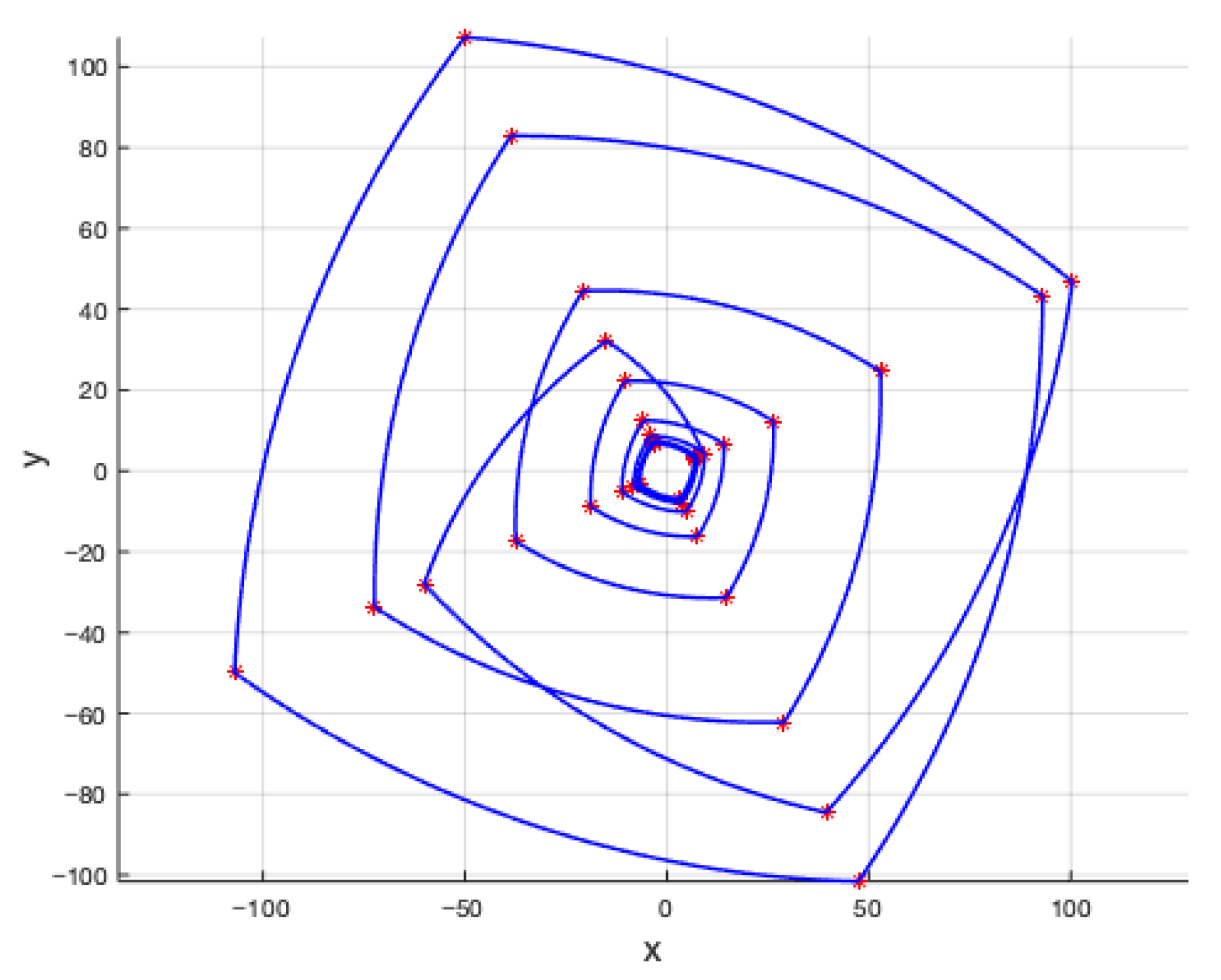
Consider the linear discrete-time dynamic system of dimension $d$: $x_{n+1}=B_n{x}_n$ with $x_0\in {\mathit{R}}_{+}^d$ and ${\left\{B_n\right\}}_0^{\infty }\subset {\mathit{R}}_{-}^{d\times d}$. Note that, with the above conditions, $x_{0_i}\ne 0$; $\forall i\in \bar{d}$, ${\left(B_n\right)}_{i,j}\ne 0$; $\forall i,j\in \bar{d}$, $\forall n\in {\mathit{Z}}_{0+}$, ${\left\{x_{2n}\right\}}_{n=0}^{\infty }\subset {\mathit{R}}_{+}^d$ and ${\left\{x_{2n+1}\right\}}_{n=0}^{\infty }\subset {\mathit{R}}_{-}^d$ so that the mapping which generates solution sequences is cyclic with $p=2$. This situation is the one to be discussed more in detail later on. However, note that if $x_0\in {\mathit{R}}_{-}^d$, ${\left\{B_{2n}\right\}}_0^{\infty }\subset {\mathit{R}}_{-}^{d\times d}$ and ${\left\{B_{2n+1}\right\}}_0^{\infty }\subset {\mathit{R}}_{+}^{d\times d}$ then ${\left\{x_{2n}\right\}}_{n=0}^{\infty }\subset {\mathit{R}}_{-}^d$ and ${\left\{x_{2n+1}\right\}}_{n=0}^{\infty }\subset {\mathit{R}}_{+}^d$ In fact, if all the components of are nonzero with the same sign, all the entries of $B_0$ are also nonzero with the same sign and, furthermore, ${\mathit{sgn}\left(B_{n+1}\right)}_{i,j}=-{\mathit{sgn}\left(B_n\right)}_{i,j}$; $\forall i,j\in \bar{d}$, $\forall n\in {\mathit{Z}}_{0+}$, then all the entries of $B_n{B}_{n+1}$ are negative for all $n\in {\mathit{Z}}_{0+}$ so that all the components of ${\left\{x_{2n}\right\}}_{n=0}^{\infty }$ have the same sign as those of $x_0$ and all the components of ${\left\{x_{2n+1}\right\}}_{n=0}^{\infty }$ has a reversed sign compared to that of the components of $x_0$. It turns out that the composed operator $B_n{B}_{n+1}$ is cyclic with a period $p=2$. This situation is discussed in the next section with numerical simulations.

Now, assume that ${\left\{{‖B‖}_n\right\}}_0^{\infty }\subset \left(0\hspace{0.33em},\hspace{0.33em}\bar{K}\right]$, for a vector-induced matrix norm $‖A‖=\underset{‖z‖=1}{sup}‖Az‖$ (since norms of matrices and vectors have to be compatible to operate with them in the sequel), which has a subsequence ${\left\{{‖B‖}_{n_k}\right\}}_{k=0}^{\infty }\subset {\left\{{‖B‖}_n\right\}}_{n=0}^{\infty }$, such that the following conditions hold:

$$C. \left(a\right) {\left\{{‖B‖}_{n_k}\right\}}_{k=0}^{\infty }\subset \left(0\hspace{0.33em},\hspace{0.33em}{\rho }_{n_k}\right]\subset \left(0,\rho \right]\subset \left(0,\hspace{0.33em}1\right);\left({\prod }_{j=n_{n_k}}^{n_{k+1}-1}\left[‖B_j‖\right]\right)<1$$

$$C. \left(b\right) ‖x_{n+1}-x_n‖\le K_n‖x_n-x_{n-1}‖\le \bar{K}‖x_n-x_{n-1}‖;\forall n\in {\mathit{Z}}_{+},$$

with ${\left\{n_k\right\}}_{k=0}^{\infty }$ being a strictly increasing sequence of non-negative integer numbers with $\left(n_{k+1}-n_k\right)\le N<+\infty$; $\forall k\in {\mathit{Z}}_{0+}$ with $n_0\in {\mathit{Z}}_{0+}$ being finite.

Assume that $X\subset {\mathit{R}}^d$ is the space of solutions and $d:X\times X\to {\mathit{R}}_{0+}^d$ is the norm-induced metric. Note that ${\left\{B_{2n}\right\}}_{n=0}^{\infty }\subset {\mathit{R}}_{+}^{d\times d}$, ${\left\{B_{2n+1}\right\}}_{n=0}^{\infty }\subset {\mathit{R}}_{-}^{d\times d}$, ${\left\{x_{2n}\right\}}_{n=0}^{\infty }\subset {\mathit{R}}_{+}^d$. Identify $A_1={\mathit{R}}_{0+}^d=cl{\mathit{R}}_{+}^d$; $A_2={\mathit{R}}_{0-}^d=cl{\mathit{R}}_{-}^d$ which are obviously closed unbounded and non-disjoint with $D=d\left({\mathit{R}}_{+}^d\hspace{0.33em},\hspace{0.33em}{\mathit{R}}_{-}^d\right)=d\left(A_1\hspace{0.33em},\hspace{0.33em}{A}_2\right)=0$ since $0\left(\in {\mathit{R}}^d\right)={\mathit{R}}_{+}^d\cap {\mathit{R}}_{-}^d=A_1\cap A_2$.

The difference equation which describes the discrete-time system is defined by a mapping $T:A_1\cup A_2\to A_1\cup A_2$ $T\left(x\right)=y$; $\forall x\in A\cup B$ which is cyclic since $T\left(A_1\right)\subset A_2$ and $T\left(A_2\right)\subset A_1$.

It turns out by using the conditions C. (a) and C. (b) that

$$\begin{gathered} ‖x_{n_{k+1}}-x_{n_k}‖=‖\left(\prod _{j=n_{n_k}}^{n_{k+1}-1}\left[B_j\right]\right)x_{n_k}-x_{n_k}‖=‖\left(I_d-\left(\prod _{j=n_{n_k}}^{n_{k+1}-1}\left[B_j\right]\right)\right)x_{n_k}‖ \\ \le \widehat{K}\left(n_k,n_{k+1}\right)‖x_{n_k}-x_{n_{k-1}}‖=\widehat{K}\left(n_k,n_{k+1}\right)‖\left(I_d-\left({\prod }_{j=n_{n_k-1}}^{n_k-1}\left[B_j\right]\right)\right)x_{n_{k-1}}‖ \\ \le \widehat{K}\left(n_k,n_{k+1}\right)\left(1-\left({\prod }_{j=n_{n_k-1}}^{n_k-1}\left[‖B_j‖\right]\right)\right)‖x_{n_{k-1}}‖\le {\rho }_{n_{k-1}}\left(1-\left({\prod }_{j=n_{n_k}}^{n_{k+1}-1}\left[‖B_j‖\right]\right)\right)‖x_{n_{k-1}}‖ \end{gathered}$$

provided that

$$1>\rho \ge {\rho }_{n_{k-1}}\ge {\displaystyle \frac{\widehat{K}\left(n_k,n_{k+1}\right)\left(1-\left({\prod }_{j=n_{n_{k-1}}}^{n_k-1}\left[‖B_j‖\right]\right)\right)}{1-\left({\prod }_{j=n_{n_k}}^{n_{k+1}-1}\left[‖B_j‖\right]\right)}}\Rightarrow \widehat{K}\left(n_k,n_{k+1}\right)\le {\rho }_{n_{k-1}}{\displaystyle \frac{1-\left({\prod }_{j=n_{n_k}}^{n_{k+1}-1}\left[‖B_j‖\right]\right)}{1-\left({\prod }_{j=n_{n_{k-1}}}^{n_k-1}\left[‖B_j‖\right]\right)}}$$

with

$$\widehat{K}\left(n_k,n_{k+1}\right)=\prod _{j=n_k}^{n_{k+1}-1}\left[K_j\right]=\left\{\begin{array}{c}{K}_{n_{k+1}-1}\left({\displaystyle \prod _{j=n_k}^{n_{k+1}-2}}\left[K_j\right]\right)\hspace{1em}if\hspace{0.33em}\hspace{0.33em}{n}_{k+1}>n_k+1\\ K_{n_{k+1}-1}\hspace{1em}if\hspace{0.33em}\hspace{0.33em}{n}_{k+1}=n_k+1\end{array}\right.$$

which is guaranteed if the following condition hold:

$$C. (c) K_{n_{k+1}-1}\le {\displaystyle \frac{{\rho }_{n_{k-1}}\left(1-\left({\prod }_{j=n_{n_k}}^{n_{k+1}-1}\left[‖B_j‖\right]\right)\right)}{\left({\prod }_{j=n_k}^{n_{k+1}-2}\left[K_j\right]\right)\left(1-\left({\prod }_{j=n_{n_{k-1}}}^{n_k-1}\left[‖B_j‖\right]\right)\right)}}\le \widehat{K}<1$$

Theorem 2 holds which is now verified. Define the following pseudo-orthogonality condition $\perp \subset X\times X$ and define ${\widehat{x}}_{n_k}=\left(x_{n_k},x_{n_k+1}\right)\in {\mathit{R}}^d\times {\mathit{R}}^d$ with $x_0\in {\mathit{R}}^d$, $x_1=B_0{x}_0$, with $x_{0_i}\ne 0$; $\forall i\in \bar{d}$. Then, the common best proximity point between $A_1$ and $A_2$ is a singleton $A_{10}=A_{20}=\left\{0\in {\mathit{R}}^d\right\}$, $‖x_{n_{k+1}}-x_{n_k}‖\to 0$ as $k\to \infty$, $x_{n_{k+1}}\perp x_{n_k}$; $\forall k\in {\mathit{{\rm Z}}}_{0+}$, so that all the consecutive elements of the subsequences ${\left\{x_{n_k}\right\}}_{k=0}^{\infty }$ are pair-wise pseudo-orthogonal (then the self-mapping $T$ on $A\cup B$ is $\perp$-preserving) and the subsequences are $PO$-sequences for any initial condition $x_0\in {\mathit{R}}^d$, ${\left\{x_{n_k}\right\}}_{k=0}^{\infty }\to 0\left(\in {\mathit{R}}^d\right)$ and then $0\in {\mathit{R}}^n$ is the unique $PO$-set, pseudo-orthogonal to any element of ${\mathit{R}}^d$. The sub-sequences ${\left\{x_{n_k}\right\}}_{k=0}^{\infty }$ are also Cauchy $PO-$ sequences since

$$\sum _{j=m}^{m+\mathcal{l}}‖x_{n_{j+1}}-x_{n_j}‖\le \left(\sum _{j=0}^{m+\mathcal{l}}{\widehat{K}}^j\right)‖x_{n_{m+1}}-x_{n_m}‖={\displaystyle \frac{1-{\widehat{K}}^{m+\mathcal{l}-1}}{1-\widehat{K}}}‖x_{n_{m+1}}-x_{n_m}‖\le {\displaystyle \frac{1}{1-\widehat{K}}}‖x_{n_{m+1}}-x_{n_m}‖$$

Then assume that for some $\epsilon =\epsilon \left(n_m\right)\in {\mathit{R}}_{+}$ such $‖x_{n_{m+1}}-x_{n_m}‖\le \epsilon$ for any given $m,\mathcal{l}\in {\mathit{Z}}_{+}$ and $\mathcal{l}\in {\mathit{Z}}_{+}$, there is some $PO$-subsequence ${\left\{x_{n_k}\right\}}_{k=0}^{\infty }$ which is not Cauchy so that there exists at least one integer $n_j\in \left[n_{m+1}\hspace{0.33em},\hspace{0.33em}{n}_{m+\mathcal{l}}\right]$ such that $‖x_{n_{j+1}}-x_{n_j}‖>\epsilon$. Then,

$$\mathcal{l}\epsilon <\sum _{j=m}^{m+\mathcal{l}}‖x_{n_{j+1}}-x_{n_j}‖\le {\displaystyle \frac{\epsilon }{1-\widehat{K}}}\Rightarrow \mathcal{l}<{\displaystyle \frac{\epsilon }{1-\widehat{K}}}$$

and that constraint is violated by the choice $\mathcal{l}\ge \left(\min z\in {\mathit{Z}}_{+}:z\ge \epsilon /\left(1-\widehat{K}\right)\right)$, hence a contradiction. As a result, all the pseudo-orthogonal subsequences are Cauchy sequences. Also, since they are convergent, they are guaranteed to be bounded. Since $x_{n_k}\to 0$ as $k\to \infty$ then $x_{n+1}=\left({\prod }_{j=n_k}^n{B}_j\right)x_{n_k}\to 0$ for any $n\in \left[n_k\hspace{0.33em},\hspace{0.33em}{n}_{k+1}-1\right]\cap {\mathit{Z}}_{+}$. Then, the whole sequence ${\left\{x_n\right\}}_{n=0}^{\infty }$ converges. Furthermore, ${\prod }_{j=n_k}^n‖B_j‖\le \underset{k\in {\mathit{Z}}_{0+}}{sup}\left({\prod }_{j=n_k}^{n_{k+1}-1}‖B_j‖\right)\le {\bar{K}}^{n_{k+1}-n_k}\le {\bar{K}}^N<+\infty$ and for any $n\in \left[n_k\hspace{0.33em},\hspace{0.33em}{n}_{k+1}-1\right]\cap {\mathit{Z}}_{+}$ and any $k\in {\mathit{Z}}_{0+}$, one has that $x_n$ is bounded so that ${\left\{x_n\right\}}_{n=0}^{\infty }$ is bounded.

On the other hand, note that the convergence of all the pseudo-orthogonal subsequences to a best proximity set in which a singleton in one of the subsets of the cyclic disposal (Theorem 2) is not a strict requirement for the results to hold. It could be replaced by all the pseudo-orthogonal subsequences being required to converge to the same proximity point (provided that it is not unique) in one of the subsets. However, the assumption that $A_{i0}=\left\{z_i\right\}$ for some $i\in \bar{p}$ of Theorem 2 leads to a direct condition for the convergence of all the relevant subsequences.

A direct extension of Theorem 2 is the following one which relaxes Condition C.3 since it only requires convergence to a particular best proximity point, even if non-unique.

Corollary 1. 

Theorem 2 also holds if all the subsequences ${\left\{T^{n_k+\mathcal{l}\left(n_k,j,i\right)}x\right\}}_{k=0}^{\infty }\left(\subset A_i\right)\to z_i\left(\in A_{i0}\right)$ for any given $x\in A_j$, any $j\in \bar{p}$, some $i\in \bar{p}$ and some $\mathcal{l}\left(n_k,j,i\right)\in \overline{p-1}\cup \left\{0\right\}$ (without requiring that $A_{i0}$ be a singleton $\left\{z_i\right\}$).

The subsequent result integrates Theorems 1 and 2 when the metric space is a uniformly convex Banach space with one of its subsets $A_i$ of the cyclic disposal being boundedly compact and whose best proximity set $A_{i0}$ is a singleton $\left\{z_i\right\}$ for some $i\in \bar{p}$. In this case, all the sequences of the boundedly compact subset (having each necessarily to have a convergent subsequence from the boundedly compactness assumption) whose distances between adjacent subsets converge to $D$ are proved to converge to such a unique best proximity point. As a result the condition C.3 of Theorem 2 is not invoked in this case since all the pseudo-orthogonal sequences in $A_i$ converge to $z_i$ for such an $i\in \bar{p}$.

Corollary 2. 

Let $\left(X,‖.‖\right)$ be a uniformly convex Banach space with a set of p nonempty and closed subsets $A_i\subset X$; $\forall i\in \bar{p}$ and $T:{\bigcup }_{i\in \bar{p}}{A}_i\to {\bigcup }_{i\in \bar{p}}{A}_i$ is a $p\left(\ge 2\right)$-cyclic self-mapping under conditions C.1–C.2 of Theorem 1. The following properties hold:

(i) 

Theorem 1 holds for $\left(X,‖.‖\right)$ with $d:X\times X\to {\mathit{R}}_{0+}$ being the $‖.‖$-induced metric.

(ii) 

Assume, furthermore, that $A_i$ is boundedly compact for some $i\in \bar{p}$ such that its best proximity set is a singleton, that is, $A_{i0}=\left\{z_i\right\}$, and that

$$D=dist\left(A_i\hspace{0.33em},\hspace{0.33em}{A}_{i+1}\right)=d\left(A_i\hspace{0.33em},\hspace{0.33em}{A}_{i+1}\right)=\underset{\theta \in A_{i+\mathrm{1,0}}}{inf}‖z_i-\theta ‖>0;\forall i\in \bar{p},$$

where $d:X\times X\to {\mathit{R}}_{0+}$ is the $‖.‖$-induced metric. Then, Theorem 2 holds for the $POMS$$\left(X,‖.‖,\perp \right)$, where the pseudo-orthogonality relation $\perp \subset X\times X$ is defined by (28) and such that $d:X\times X\to {\mathit{R}}_{0+}$ is the $‖.‖$-induced metric.

Proof. 

Property (i) holds directly since the uniformly convex metric space $\left(X,‖.‖\right)$ is also a metric space under the norm-induced metric. By hypothesis, $A_i$ is boundedly compact and $A_{i0}=\left\{z_i\right\}$ for some $i\in \bar{p}$. Since $A_i$ is nonempty, closed and boundedly compact, any bounded subsequences in $A_i$, according to Theorem 1 (ii), are also convergent in $A_i$, that is, ${\left\{T^{n_k+\mathcal{l}\left(n_k,j,i\right)}x\right\}}_{k=0}^{\infty }\left(\subset A_i\right)\to {\omega }_i\in A_i$; $\forall x\in A_j$, $\forall j\in \bar{p}$ from Theorem 1 (ii) for some sequence of integers $\mathcal{l}\left(n_k,j,i\right)$ in $\left[0,p-1\right]$. Assume that the limit ${\omega }_i\notin A_{i0}$ so that $‖{\omega }_i-T{\omega }_i‖=d\left({\omega }_i,\hspace{0.33em}T{\omega }_i\right)>D$. Then, Theorem 1 (i) fails since $D\leftarrow ‖T^{n_k+\mathcal{l}\left(n_k,j,i\right)}x-T^{n_k+\mathcal{l}\left(n_k,j,i\right)+1}x‖\to ‖{\omega }_i-T{z}_i‖>D$ as $k\to \infty$, hence a contradiction to Property (i). Therefore,${\omega }_i=z_i$, then, for any given $x\in A_j$, any $j\in \bar{p}$, some $i\in \bar{p}$ such that $A_{i0}=\left\{z_i\right\}$ and some $\mathcal{l}\left(n_k,j,i\right)\in \overline{p-1}\cup \left\{0\right\}$, one has that Condition C.3 of Theorem 2 holds, that is, ${\left\{T^{n_k+\mathcal{l}\left(n_k,j\hspace{0.17em},i\right)}x\right\}}_{k=0}^{\infty }\left(\subset A_i\right)\to A_{i0}=\left\{z_i\right\}$. As a result, Theorem 2 holds so that Property (ii) is proved. □

Note that Corollary 2 (ii) concludes, in particular, that the following properties hold:

$$‖T^{n_k+\mathcal{l}\left(n_k,j,i\right)}x-T^{n_k+\mathcal{l}\left(n_k,j,i\right)+1}x‖\to D; \forall x\in A_j, \forall j\in \bar{p},$$

$$‖T^{pn\left(n_k+\mathcal{l}\left(n_k,j,i\right)\right)}x-T^{pm\left(n_k+\mathcal{l}\left(n_k,j,i\right)\right)+1}x‖\to D, ‖T^{pn\left(n_k+\mathcal{l}\left(n_k,j,i\right)\right)}x-T^{pm\left(n_k+\mathcal{l}\left(n_k,j,i\right)\right)}x‖\to 0; \forall n,m\in {\mathit{Z}}_{+}, \forall x\in A_j, \forall j\in \bar{p},$$

$$‖T^{pn\left(n_k+\mathcal{l}\left(n_k,j,i\right)\right)}x‖\to z_i; ‖T^{pm\left(n_k+\mathcal{l}\left(n_k,j,i\right)\right)+1}x‖\to T{z}_i; \forall n,m\in {\mathit{Z}}_{+}, \forall x\in A_j, \forall j\in \bar{p}.$$

The following result is obvious from an extended Theorem 2 for the case that the subsets $A_i$ pair-wise intersect so that the distance between adjacent subsets is null.

Corollary 3. 

Theorem 2 can be directly extended to the case when $A_i\cap A_{i+1}=\left\{z_i\right\}$; $\forall i\in \bar{p}$ implying that $D=0$.

The next result relies on some further properties related to the whole sequences ${\left\{T^{n}x\right\}}_{n=0}^{\infty }$ for $x\in {\bigcup }_{i\in \bar{p}}{A}_i$, which can be obtained from the properties which have been proved in Theorem 1 for their relevant subsequences under Conditions C.1–C.2, and, furthermore in Theorem 2 under the extra Condition C.3.

Theorem 3. 

Under the hypotheses of Theorem 1, the following additional properties to those proved in Theorem 1 hold for the whole sequence generated through the self-mapping T on ${\bigcup }_{i\in \bar{p}}{A}_i$,

(i) 

The sequences ${\left\{T^{n+j}x\right\}}_{n=0}^{\infty }$ and ${\left\{T^{pn+j}x\right\}}_{n=0}^{\infty }$ are bounded; $\forall x\in {\bigcup }_{i\in \bar{p}}{A}_i$, $\forall j\in \overline{p-1}\cup \left\{0\right\}$.

(ii) 

The following limits of distances exist:

$$\underset{n\to \infty }{\mathit{lim}\hspace{0.33em}}d\left(T^{n+j}x\hspace{0.33em},\hspace{0.33em}{T}^{n+j}y\right)=D; \forall \left(x,y\right)\in A_i\times A_{i+1}\cup A_{i+1}\times A_i; \forall i\in \bar{p}, \forall n\in {\mathit{Z}}_{0+}, \forall j\in \overline{p-1}\cup \left\{0\right\},$$

$$\underset{n\to \infty }{\mathit{lim}\hspace{0.33em}}d\left(T^{n+j}x\hspace{0.33em},\hspace{0.33em}{T}^{n+j+1}x\right)=D;x\in {\bigcup }_{i\in \bar{p}}{A}_i;\forall i\in \bar{p},\forall j\in \overline{p-1}\cup \left\{0\right\},\forall n\in {\mathit{Z}}_{0+}.$$

Under the additional hypothesis of Theorem 2, the following additional properties to those proved in Theorem 2 hold for the whole sequences:

(iii) 

${\left\{T^{\left(n+m\right)p}x-T^{np}x\right\}}_{n=0}^{\infty }\to 0$; $\forall x\in {\bigcup }_{i\in \bar{p}}{A}_i$, $\forall m\in {\mathit{Z}}_{0+}$,

${\left\{T^{n+j}x-T^{n+j}y\right\}}_{n=0}^{\infty }\to 0$; $\forall x,y\in A_i$, $\forall j\in \overline{p-1}\cup \left\{0\right\}$, $\forall i\in \bar{p}$,

${\left\{T^{np+i}x\right\}}_{n=0}^{\infty }\to z_{i+j}\left(=T^j{z}_i\right)$; $\forall x\in A_j$ and any $j\in \bar{p}$,

${\left\{T^{n+\mathcal{l}\left(n,j,i\right)+\sigma }x\right\}}_{n=0}^{\infty }\left(\subset A_{i+\sigma }\right)\to z_{i+\sigma }\left(=T^{\sigma }{z}_i\right)$,

$\forall x\in A_j$, $\forall j\in \bar{p}$, some $\mathcal{l}\left(n,j,i\right)\in \overline{p-1}\cup \left\{0\right\}$, $\forall \sigma \in \overline{p-1}\cup \left\{0\right\}$.

Proof. 

From Theorem 1 (ii), ${\left\{T^{n_k+j}x\right\}}_{k=0}^{\infty }$ is bounded for any given $x\in {\bigcup }_{i\in \bar{p}}{A}_i$; $\forall j\in \overline{p-1}\cup \left\{0\right\}$. Take $n\in \left[n_k\hspace{0.33em},\hspace{0.33em}{n}_{k+1}\right]$ and note that $\left(n-n_k\right)$ is finite since $\underset{k\in {\mathit{Z}}_{0+}}{sup}\left(n-n_k\right)\le \underset{k\in {\mathit{Z}}_{0+}}{sup}\left(n_{k+1}-n_k\right)\le N<+\infty$, from Condition C.2 of Theorem 1, and then $T^{n}x=T^{n-n_k}{T}^{n_k+j}x$. Define $y=T^{n-n_k}x$, note that ${\left\{T^{n_k+j}y\right\}}_{k=0}^{\infty }$ is bounded; $\forall y\in {\bigcup }_{i\in \bar{p}}{A}_i$, then one gets that ${\left\{T^{n+j}x\right\}}_{n=0}^{\infty }$ is bounded for any given $x\in {\bigcup }_{i\in \bar{p}}{A}_i$; $\forall j\in \overline{p-1}\cup \left\{0\right\}$ and Property (i) is proved concerning the boundedness of ${\left\{T^{n+j}x\right\}}_{n=0}^{\infty }$ since one has

$$d\left(T^{n}x,T^{n_k+j}x\right)=d\left(T^{n_k+j}{T}^{n-n_k}x,T^{n_k+j}x\right)\le d\left(x,T^{n_k+j}x\right)+d\left(T^{n_k+j}y,x\right)<+\infty$$

Now, since ${\left\{T^{pn+j}x\right\}}_{k=0}^{\infty }$ a subsequence of the bounded ${\left\{T^{n+j}x\right\}}_{k=0}^{\infty }$, it is also bounded so that Property (i) is fully proved.

To prove Property (ii), note from Conditions C.1–C.2 that

$$\begin{gathered} d\left(T^{n+j}x\hspace{0.33em},\hspace{0.33em}{T}^{n+j}y\right)-D\le \left(\prod _{\mathcal{l}=0}^{n-n_k-1}\left[K_{n_k+j+\mathcal{l}}\right]\right)\hspace{0.33em}\left(d\left(T^{n_k+j}x\hspace{0.33em},\hspace{0.33em}{T}^{n_k+j}y\right)-D\right) \\ \le {\bar{K}}^{n-n_k}\left(d\left(T^{n_k+j}x\hspace{0.33em},\hspace{0.33em}{T}^{n_k+j}y\right)-D\right); \\ \forall \left(x,y\right)\in A_i\times A_{i+1}\cup A_{i+1}\times A_i; \forall i\in \bar{p}, \forall n\in {\mathit{Z}}_{0+}, \forall j\in \overline{p-1}\cup \left\{0\right\}. \end{gathered}$$

Then, one has that

$$\begin{gathered} 0\le \underset{n\to \infty }{\mathit{lim}\hspace{0.33em}\mathit{sup}}\left(d\left(T^{n+j}x\hspace{0.33em},\hspace{0.33em}{T}^{n+j}y\right)-D\right)-\underset{n\to \infty }{\mathit{lim}\hspace{0.33em}}{\overline{K}}^{n-n_k}\left(d\left(T^{n_k+j}x\hspace{0.33em},\hspace{0.33em}{T}^{n_k+j}y\right)-D\right) \\ =\underset{n\to \infty }{\mathit{lim}\hspace{0.33em}\mathit{sup}}\left(d\left(T^{n+j}x\hspace{0.33em},\hspace{0.33em}{T}^{n+j}y\right)-D\right)-0\le 0 \end{gathered}$$

and then there exist the limit $\underset{n\to \infty }{\mathit{lim}\hspace{0.33em}}d\left(T^{n+j}x\hspace{0.33em},\hspace{0.33em}{T}^{n+j}y\right)=D$. By taking $y=Tx$, one has, in particular, $\underset{n\to \infty }{\mathit{lim}\hspace{0.33em}}d\left(T^{n+j}x\hspace{0.33em},\hspace{0.33em}{T}^{n+j+1}x\right)=D$; $\forall x\in {\bigcup }_{i\in \bar{p}}{A}_i$, $\forall j\in \overline{p-1}\cup \left\{0\right\}$. Property (ii) is proved.

Property (iii) follows by extending directly Theorem 2 (iii) to the whole sequences ${\left\{T^{n+j}x\right\}}_{n=0}^{\infty }\to 0$ ;  $\forall x\in A_i$ , $\forall j\in \overline{p-1}\cup \left\{0\right\}$ , $\forall i\in \bar{p}$, and ${\left\{T^{np+i}x\right\}}_{n=0}^{\infty }\to z_{i+j}\left(=T^j{z}_i\right)$; $\forall x\in A_j$ and any $j\in \bar{p}$, since $A_{i0}=\left\{z_i\right\}$ for some $i\in \bar{p}$ and Properties [(i)–(iii)] hold for the whole sequences, that is, they are bounded and the distances in adjacent subsets converge to the distance in-between such subsets. □

Some direct convergence results follow from Theorems 1 and 2 for the studied bounded sequences under further conditions for the case of real numbers under the Euclidean distance and for the case of compact metric spaces.

Corollary 4. 

Assume in Theorem 1 that $X=\mathit{R}$, $d\left(x,y\right)=\left|x-y\right|$, the Euclidean distance, for any $x,y\in \mathit{R}$, and $A_i=\left[{\underset{\_}{a}}_i,\hspace{0.33em}{\bar{a}}_i\right]\hspace{0.33em}\subset \mathit{R}$ and let $POMS$ $\left({\bigcup }_{i\in \bar{p}}{A}_i,⥂d,\hspace{0.33em}\perp \right)$ be defined, subject to the given conditions on the cyclic self-mapping $T:{\bigcup }_{i\in \bar{p}}{A}_i\to {\bigcup }_{i\in \bar{p}}{A}_i$, under the pseudo-orthogonality binary relation (28), which implies the constraint (14) under Conditions C.1–C.2, which defines the subsequences ${\left\{T^{n_k+j}x\right\}}_{k=0}^{\infty }\left(\subset {\left\{T^{n+j}x\right\}}_{k=0}^{\infty }\right)$; $\forall i\in \bar{p}$, $\forall j\in \overline{p-1}\cup \left\{0\right\}$.

Then, the following properties hold in addition to Theorem 1 [(i)–(v)]:

(i) 

Each bounded sequence ${\left\{T^{n_k+j}x\right\}}_{k=0}^{\infty }$ referred to in Theorem 1 (ii) (in turn, being a subsequence of ${\left\{T^{n+j}x\right\}}_{k=0}^{\infty }$) has a convergent subsequence ${\left\{T^{n_{k_l}+j}x\right\}}_{\mathcal{l}=0}^{\infty }$ for any given $x\in {\bigcup }_{i\in \bar{p}}{A}_i$; $\forall i\in \bar{p}$, $\forall j\in \overline{p-1}\cup \left\{0\right\}$. Then, the whole sequence ${\left\{T^{n+j}x\right\}}_{k=0}^{\infty }$ has the same convergent subsequence ${\left\{T^{n_{k_l}+j}x\right\}}_{\mathcal{l}=0}^{\infty }$ for any given $x\in {\bigcup }_{i\in \bar{p}}{A}_i$; $\forall i\in \bar{p}$, $\forall j\in \overline{p-1}\cup \left\{0\right\}$.

(ii) 

Each bounded sequence ${\left\{T^{p{n}_k+j}x\right\}}_{k=0}^{\infty }\left(\subset A_{i+j}\right)$ referred to in Theorem 1 (iv) (in turn, being a subsequence of ${\left\{T^{pn+j}x\right\}}_{k=0}^{\infty }\left(\subset A_{i+j}\right)$) has a convergent subsequence ${\left\{T^{p{n}_{k_l}+j}x\right\}}_{\mathcal{l}=0}^{\infty }\left(\subset A_{i+j}\right)$ for any given $x\in A_i$; $\forall i\in \bar{p}$, $\forall j\in \overline{p-1}\cup \left\{0\right\}$. Then, the whole sequence ${\left\{T^{np+j}x\right\}}_{k=0}^{\infty }$ has the same convergent subsequence ${\left\{T^{p{n}_{k_l}+j}x\right\}}_{\mathcal{l}=0}^{\infty }$ for any given $x\in {\bigcup }_{i\in \bar{p}}{A}_i$; $\forall i\in \bar{p}$, $\forall j\in \overline{p-1}\cup \left\{0\right\}$.

(iii) 

All the proximity subsets of the closed real intervals $A_i$, $\forall i\in \bar{p}$ to their respective adjacent subsets are nonempty and non-necessarily singletons, and contain the respective convergence points of the convergent subsequences of Properties [(i)–(ii)] which are in the pseudo-orthogonal set-element $Z$ of $\left({\bigcup }_{i\in \bar{p}}{A}_i,d,\hspace{0.33em}\perp \right)$.

Proof. 

Note that $\left({\bigcup }_{i\in \bar{p}}{A}_i,⥂d,\hspace{0.33em}\perp \right)$ is a complete pseudo-orthogonal space, since the metric space $\left(\mathit{R},d\right)$ is complete (from celebrated Bolzano-Weierstrass theorem), and that the subsequences ${\left\{T^{n_k+j}x\right\}}_{k=0}^{\infty }$ are $PO$-sequences with respect to $\perp$. From Theorem 1 (iii), each $PO$-sequence ${\left\{T^{n_k+j}x\right\}}_{k=0}^{\infty }$ is bounded for any given $x\in {\bigcup }_{i\in \bar{p}}{A}_i$; $\forall j\in \overline{p-1}\cup \left\{0\right\}$ so it has a convergent subsequence ${\left\{T^{n_{k_{\mathcal{l}}}+j}x\right\}}_{\mathcal{l}=0}^{\infty }$ in ${\bigcup }_{i\in \bar{p}}{A}_i$. Property (i) has been proved. In the same way, from Theorem 1 (iv), each $PO$-sequence ${\left\{T^{p{n}_k+j}x\right\}}_{k=0}^{\infty }\left(\subset A_{i+j}\right)$ is bounded for any given $x\in A_i$; $\forall j\in \overline{p-1}\cup \left\{0\right\}$ and has to have a subsequence ${\left\{T^{p{n}_{k_{\mathcal{l}}}+j}x\right\}}_{\mathcal{l}=0}^{\infty }\left(\subset A_{i+j}\right)$, which is, in turn, a subsequence of ${\left\{T^{p{n}_k+j}x\right\}}_{k=0}^{\infty }$, a subsequence of ${\left\{T^{pn+j}x\right\}}_{k=0}^{\infty }$, and a subsequence of ${\left\{T^{pn+j}x\right\}}_{k=0}^{\infty }$, which possesses a limit point in $A_{i+j}$. Property (ii) has been proved. Now, note from Theorem 1 (ii), that the sequences of distances between their corresponding generated points on adjacent subsets converge to $D=\left|{\bar{a}}_i-{\underset{\_}{a}}_{i+1}\right|$, if the sets are disjoint, and that $D=0$, otherwise $\forall i\in \bar{p}$. Therefore, the $p$ convergence points $z_i$ in each of the subsets $A_i$; $\forall i\in \bar{p}$ are best proximity points to their adjacent subset, so that the best proximity subsets $A_{i0}$; $\forall i\in \bar{p}$ are all non-empty, $z_i\in A_{i0}$ and the pseudo-orthogonal set-element $Z\supset {\bigcup }_{i\in \bar{p}}{A}_{i0}\supset \left\{z_1,z_2,⥂\dots ,z_p\right\}$. Property (iii) follows. □

Remark 4. 

Note that the above result by itself does not ensure that the best proximity subsets $A_{i0}$ are singletons since the limit points $z_i$ depend on the pseudo-orthogonal relation which generates the subsequences which converge to those points rather than on the subsets themselves. They can also be dependent on the initial points of the involved sequences. Therefore, it is also guaranteed that there is a best proximity point per best proximity set which is a limit point of some subsequence at each subset of the cyclic disposal.

The following result is similar to Corollary 4 for the case when $\left(X,d\right)$ is a compact metric space. Thus, $X$ is not required to be, in particular, the real set. However, since a compact metric space is both complete and totally bounded, the subsets $A_i$; $\forall i\in \bar{p}$ of the cyclic disposal have to be bounded. Note, in particular and to fix ideas, that, although the metric space $\left(\mathit{R},d\right)$ is complete, it is not compact since it is not totally bounded. Thus, the proofs of boundedness of the sequences follows directly by their construction, from the boundedness of the subsets where they belong to, so that it does not require to be specifically proved in the way as addressed in Theorem 1 which did not invoke the compactness assumption.

Corollary 5. 

Assume in Theorem 1 that $\left(X,d\right)$ is a compact metric space and let the $POMS$ $\left({\bigcup }_{i\in \bar{p}}{A}_i,\hspace{0.33em}d,\hspace{0.33em}\perp \right)$ be defined, subject to the given conditions on the cyclic self-mapping $T:{\bigcup }_{i\in \bar{p}}{A}_i\to {\bigcup }_{i\in \bar{p}}{A}_i$, with the pseudo-orthogonality relation (28), that implies the fulfillment of Conditions C.1–C.2, and which defines the subsequences ${\left\{T^{n_k+j}x\right\}}_{k=0}^{\infty }\left(\subset {\left\{T^{n+j}x\right\}}_{k=0}^{\infty }\right)$; $\forall i\in \bar{p}$, $\forall j\in \overline{p-1}\cup \left\{0\right\}$. Then, the properties of Corollary 4 hold.

5. Numerical Examples

This section contains some numerical examples to illustrate the theoretical results and conceptual examples discussed in the previous sections. In particular, this section is organized into two parts: in the first one, the concept of pseudo-orthogonality, introduced in Section 3 in its application to dynamical systems, will be illustrated numerically while in the second part, the results of Theorems 2 and 3 concerning cyclic self-maps will be illustrated through the numerical simulation of Example 16 and an additional example.

5.1. Pseudo-Orthogonality Relation Applied to the Stability of Dynamical Systems

We now apply the definition of pseudo-orthogonality introduced in Section 3 to dynamical systems, and we present the construction of pseudo-orthogonal sequences. To this end, the starting point will be Example 7, which refers to a continuous dynamical system. Let us consider the system given by (1), where n = 3, and the dynamics matrix is

$$A=\left[\begin{array}{ccc}-3& 2& -2\\ -2& 0& -3\\ 2& -1& -2\end{array}\right]$$

with the initial condition x₀ = [5, −6, 7]. The eigenvalues of A are {−1 + 2i, −1 − 2i, −3}, and therefore A is a stable (Hurwitz) matrix. The system trajectories corresponding to each of the states are shown in Figure 1a. It can be observed that the system exhibits oscillatory trajectories that converge to zero. Consequently, the 2-norm of the state, shown in Figure 1b, also displays oscillations, and although it converges to zero, the convergence is not monotonic.

Given a sequence of time instants {t_i}, we can define the pseudo-orthogonality relation between two states x(t_i,x₀) and x(t_i+1,x₀) as $x\left(t_i,x_0\right)\perp x\left(t_{i+1},x_0\right)$ if $‖x\left(t_{i+1},x_0\right)‖<‖x\left(t_i,x_0\right)‖$ if $x\left(t_i,x_0\right)\ne 0$ and $‖x\left(t_{i+1},x_0\right)‖=‖x\left(t_i,x_0\right)‖=0$. In this way, we can define a sequence of states related by pseudo-orthogonality as the sequence formed by those states that, at a given instant, have a strictly smaller norm than at the previous instant. With this definition, the states related by pseudo-orthogonality are represented in Figure 2 by red asterisks. As observed in Figure 2, this definition of pseudo-orthogonality does not, by itself, generate monotonically decreasing sequences, since positive jumps in the norm may occur due to the oscillatory nature of the system. This relation is understood as the state norm at a given instant being smaller than the state norm at the previous instant. However, from this pseudo-orthogonality sequence, one can extract a pseudo-orthogonal subsequence that is indeed monotonically decreasing, as shown in Figure 3 and discussed in Example 7, for an appropriate choice of the time instants {t_i}. From the previously defined pseudo-orthogonal sequence, a monotonically decreasing subsequence is extracted in that figure, consisting of the points that maintain a pseudo-orthogonality relation with all preceding states. The monotonically decreasing pseudo-orthogonal sequence is associated with a suitable choice of the sequence of instants {t_i} at which the pseudo-orthogonality relation is evaluated. In this sense, one could define the strict pseudo-orthogonality of a sequence of states as the sequence formed by those states that are pseudo-orthogonal to all preceding states. Verifying the strict pseudo-orthogonality relation yields sequences that are monotonically decreasing in norm.

On the other hand, Example 9 discusses the concept of pseudo-orthogonality for discrete-time systems. Let us consider system (3) with the dynamics matrix given by

$$A=\left[\begin{array}{ccc}0.6& 0.8& 0.3\\ -0.7& 0.6& 0.2\\ 0.2& -0.5& 0.5\end{array}\right]$$

with the same initial condition as before. The eigenvalues of this matrix are {0.7287, 0.4857 + 0.7851i, 0.4857 − 0.7851i}, and since all of them have absolute value smaller than one, the matrix is stable (Schur). The presence of complex eigenvalues in the spectrum indicates the oscillatory behavior of the states, as shown in Figure 4a. The oscillation in the states is reflected in oscillations in the state norm, as seen in Figure 4b.

Note that both the states and the norm exhibit oscillations, and their convergence to zero is not monotonic. The state values at each iteration have been interpolated with straight lines to more clearly illustrate the system’s oscillatory behavior in the plot. Using the same definition of pseudo-orthogonality as for the continuous case, the sequence of states that satisfy the pseudo-orthogonality relation is shown in Figure 5. Due to the oscillatory nature of the system, not all states satisfy the pseudo-orthogonality relation, and they do not form a monotonically decreasing sequence. Note that the state norm at a given instant is smaller than the norm at the previous instant. However, from this sequence, a strictly pseudo-orthogonal subsequence (defined as before) can be extracted, which is monotonically decreasing. Figure 6 displays the states that maintain a strict pseudo-orthogonality relation, in the sense that each state is pseudo-orthogonal to all preceding states, resulting in monotonically decreasing sequences.

It is worth noting that the stability of a dynamical system can be reformulated in both cases through the existence of a strictly pseudo-orthogonal sequence, that is, monotonically decreasing. That is, a dynamical system is asymptotically stable if and only if there exists a monotonically decreasing pseudo-orthogonal sequence (strictly pseudo-orthogonal, in the sense that it is formed by pseudo-orthogonal elements to all preceding states). Therefore, as an alternative to the traditional stability conditions for dynamical systems, one can consider the requirement for the existence of such pseudo-orthogonal sequences, which may lead to new stability criteria that could be useful in various contexts. In particular, as a direct consequence of interpreting stability in terms of strictly pseudo-orthogonal sequences, it can be concluded that the discrete system (3) is asymptotically stable if and only if there exists an N such that $‖A^N‖<1$, a well-known condition in control theory usually derived from alternative arguments.

5.2. Pseudo-Orthogonality in p-Cycling Mappings

In this section, we study a numerical example of the concept of pseudo-orthogonality applied to cyclic mappings in order to illustrate the results of Theorems 2 and 3. To this end, the starting point will be Example 16 from Section 4. Let us consider the discrete dynamical system x_n+1 = B_n x_n with d = 3, defined as

$$A_{2n}=f\left(n\right)\left[\begin{array}{ccc}0.3& 0.5& 0.1\\ 0.1& 0.4& 0.5\\ 0.4& 0.2& 0.3\end{array}\right]; A_{2n+1}=-g\left(n\right)\left[\begin{array}{ccc}0.2& 0.5& 0.1\\ 0.1& 0.2& 0.5\\ 0.4& 0.1& 0.2\end{array}\right]$$

with $f\left(n\right)=1+\left(0.5n+0.5n^2+0.3n^3+0.4n^4\right)0.35^n$ and $g\left(n\right)=1+\left(0.35n+0.25n^2+0.4n^3\right)0.25^n$. As can be seen, the dynamics matrix components change sign at each iteration, as designed in Example 16. Moreover, we have $\underset{n\to \infty }{lim}f\left(n\right)=\underset{n\to \infty }{lim}g\left(n\right)=1$, so that the eigenvalues of A_2n and A_2n+1 are, asymptotically, {0.9383, 0.0309 + 0.2848i, 0.0309 − 0.2848i} and {−0.7647, 0.0823 + 0.3149i, 0.0823 − 0.3149i}, respectively, while their 2-norms converge asymptotically to 0.9445 and 0.7713. The state trajectory is shown in Figure 7. In this figure, it can be observed that the state values initially increase before decreasing and converging to zero. This trajectory occurs because, initially, the dynamics matrices produce unstable behavior since for low iteration values the dynamics matrices have eigenvalues outside the unit circle. In fact, when n = 1, the dynamics matrix has eigenvalues {1.1728, 0.0386 + 0.356i, 0.0386 − 0.356i}, and for n = 2, {−1.87, 0.2014 + 0.77i, 0.2014 − 0.77i}. Furthermore, Figure 7 also shows the oscillatory behavior of the system due to the sign change. The dynamical system can be represented as a cyclic mapping every two iterations, where all components of the state switch from positive to negative values and vice versa.

Since $\underset{n\to \infty }{lim}f\left(n\right)=\underset{n\to \infty }{lim}g\left(n\right)=1$ there exists a non-negative integer n₀ such that for all $n\ge n_0$, the dynamics matrices have a norm smaller than one, and the contractivity conditions of Theorem 2 are satisfied, as verified in Example 16 through conditions C. (a) and C. (b). Moreover, the only pseudo-orthogonal point in both subsets is the origin, (0, 0, 0). The evolution of the state norm is shown in Figure 8. It can be seen that the state norm increases for some iteration values and decreases for others. We explicitly construct the pseudo-orthogonal sequence by starting from an initial state $x\left(t_0\right)=x_0$ and iteratively adding $x\left(t_{i+1}\right)$ whenever its norm is strictly smaller than that of the previously selected state, i.e., $‖x\left(t_{i+1}\right)‖<‖x\left(t_{i_k}\right)‖$. Using the pseudo-orthogonality relation defined in Example 16, Figure 9a shows the instants corresponding to the states that satisfy this pseudo-orthogonality relation within the sequence of norm values. From this pseudo-orthogonal sequence, a subsequence (called the strictly pseudo-orthogonal sequence) can be selected in which the norm is monotonically decreasing. Figure 9b shows the points of this strictly pseudo-orthogonal sequence. Finally, Figure 10 shows the sequence of distances between consecutive states. As observed in Figure 10, the distance sequence converges to zero, corresponding to a Cauchy sequence, as concluded in Theorems 2 and 3. The existence of pseudo-orthogonal sequences converging to the unique common pseudo-orthogonal point is equivalent to the asymptotic stability condition of the dynamical system.

To conclude this section, we consider the example of the cyclic rotation operator in the plane, rotating counterclockwise by 90 degrees with variable amplitude, given by

$$x_{n+1}=A_n{x}_n; A_n=h\left(n\right)\left[\begin{array}{cc}0& -1\\ 1& 0\end{array}\right]$$

with $h\left(n\right)=\left(1+0.5n+2.5n^2\right){0.7}^n$. Starting from an initial condition, the operator rotates counterclockwise the point’s position by 90 degrees in each iteration and changes its distance to the origin according to the function h(n). In this sense, it is a cyclic operator, with the four quadrants of the plane forming the cycle of spaces. Figure 11 shows the solution trajectory of the iterations in the plane, where the initial point is located 10 units from the origin and at an angle of 25 degrees with respect to the horizontal axis.

For this operator, four sets can be defined as A₁, A₂, A₃, and A₄ corresponding to the four open quadrants of the plane. The intersection of the closures of these sets is the origin (0, 0), which is the only common pseudo-orthogonal point. It can be observed that $\underset{n\to \infty }{lim}h\left(n\right)=0$, and consequently, there exists a non-negative integer n₀ such that for all $n\ge n_0$, the norm of A_n satisfies the contraction condition of Theorem 2. Moreover, Figure 11 shows that some motion trajectories intersect at certain iterations, indicating that the distance to the origin can increase or decrease at each iteration, although it asymptotically tends to zero. Figure 12 shows the evolution of the state norm. Using the pseudo-orthogonality relation defined in Example 16, we can define a sequence of pseudo-orthogonal points related through a decrease in the norm, as well as a monotonically decreasing sequence, which are shown in Figure 13, as in the previous examples.

Therefore, the contractivity condition gives rise to a pseudo-orthogonal sequence that converges to the unique common pseudo-orthogonal point, which is the origin (0, 0), as predicted by Theorem 2. Moreover, the sequence of states in each space A₁, A₂, A₃, and A₄ forms a Cauchy sequence, as stated in Theorem 3. This is illustrated in Figure 14, which shows how the distance between successive points belonging to the same space $A_i$ converges to zero.

If the function h(n) is now changed to $h\left(n\right)=\left(1+0.5n+2.5n^2\right){0.7}^n+0.75$, then the iteration points will no longer converge to the origin, but to a best proximity point within each set. Thus, in this case D > 0, as is shown in Figure 15, in contrast to the behavior shown in Figure 11. Moreover, the evolution of the state norm is shown in Figure 16 for this case, where it is observed that it is not converging to zero. However, the sequences still exhibit the cauchyness property, as shown in Figure 17, for the iterations contained in the first quadrant, as a matter of example.

6. Conclusions

The main research findings and novel contributions of this article are summarized as follows:

• Concept and Definition of Pseudo-Orthogonality and Pseudo-Orthogonal Metric Spaces. The article introduces and formalizes a new proposed non-symmetric orthogonality relation, termed pseudo-orthogonality, together with some illustrative examples that motivate its use. By endowing a metric space with this relation, the paper defines pseudo-orthogonal metric spaces, a new structural framework tailored for the analysis of cyclic self-mappings.
• Best Proximity Points via Convergence of Pseudo-Orthogonal Sequences (New Convergence Framework). A key contribution is the development of an iteration-dependent contractive condition that selects pseudo-orthogonal subsequences from general cyclic iterates, even when the full sequences may be locally non-contractive or even locally expansive. Using this mechanism, the paper proves the existence of best proximity points for cyclic mappings and establishes the convergence of the selected sequences within each subset of the cyclic structure. This analysis also shows that the resulting pseudo-orthogonal metric subspace is complete, even without assuming completeness of the ambient space.
• Connection with Stability Theory. The study reveals how pseudo-orthogonality naturally arises in stability and controllability problems in dynamic systems, bridging fixed-point methods with system theory. The pseudo-orthogonality condition provides a new tool for selecting dynamically meaningful sequences, which serves as the backbone for the convergence and proximity results established in the paper.

References

1. Eldred, A.A.; Veeramani, P. Existence and convergence of best proximity points. J. Math. Anal. Ap-Plications 2006, 323, 1001–1006. [Google Scholar] [CrossRef]
2. Karpagam, S.; Agrawal, S. Best proximity point theorems for p-cyclic Meir-Keeler contractions. Fixed Point Theory Appl. 2009, 2009, 197308. [Google Scholar] [CrossRef]
3. Aslantas, M.; Sahin, H.; Altun, I. Best proximity point theorems for cyclic p-contractions with some consequences and ap-plications. Nonlinear Anal. Model. Control. 2021, 26, 113–129. [Google Scholar] [CrossRef]
4. Khandani, H.H.; Vaezpour, S.M.; Sims, B. Common fixed points of generalized multivalued contraction in complete metric spaces. J. Comput. Anal. Appl. 2011, 13, 1025–1038. [Google Scholar]
5. Khan, A.R.; Gürsoy, F.; Karakaya, V. Jungck-Khan iterative scheme and higher convergence rate. Int. J. Comput. Math. 2016, 93, 2092–2105. [Google Scholar] [CrossRef]
6. Espínola, R.; Fernandez-Leon, A. On best proximity points in metric and Banach spaces. Can. J. Math. 2011, 63, 533–5550. [Google Scholar] [CrossRef]
7. Eldred, A.A.; Kirk, W.A.; Veeramani, P. Proximal normal structure and relatively nonexpansive mappings. Stud. Math. 2005, 171, 283–294. [Google Scholar] [CrossRef]
8. Phatak, H.K.; Shahzad, N. Some results on best proximity points for cyclic mappings. Bull. Belg. Math. Soc. Simon Stevin 2013, 20, 559–572. [Google Scholar]
9. Fulatan, I.A.; Yahaya, S.; Imam, A.T. Best proximity points for nonlinear cyclic mappings on multiplicative metric spaces. Niger. J. Sci. Res. 2016, 15, 587–590. [Google Scholar]
10. Fallahi, K.; Rad, G.S. Best proximity points theorem in b-metric spaces endowed with a graph. Fixed Point Theory 2020, 21, 465–474. [Google Scholar] [CrossRef]
11. Weng, S.; Liu, X.; Chao, Z. Some fixed point theorems for cyclic mapping in a complete b-metric-like space. Results Nonlinear Anal. 2020, 3, 207–213. [Google Scholar]
12. Gupta, V.; Mani, N.; Ansari, A.J.; Kumari, S. Some fixed point results on C-class functions for generalized cyclic contractive mappings in b-metric spaces. Math. Comput. Sci. 2025, 6, 19–29. [Google Scholar]
13. Kumari, P.S.; Panthi, D. Connecting various types of cyclic contractions and contractive self-mappings with Hardy-Rogers self-mappings. Fixed Point Theory Appl. 2016, 2016, 15. [Google Scholar] [CrossRef]
14. Gabeleh, M.; Patle, P.R. Best proximity point (pair) results via MNC in Busemann convex metric spaces. Appl. Gen. Topol. 2022, 23, 405–424. [Google Scholar] [CrossRef]
15. Wu, D.; Weng, S. A fixed point result involving BSS-type cyclic mapping. J. Physics. Conf. Ser. 2025, 2964, 012101. [Google Scholar] [CrossRef]
16. Bassou, A.; Sabar, T.; Mohamed, A. A note on best proximity point for S-cyclic mappings. Fixed Point Theory 2021, 22, 75–82. [Google Scholar] [CrossRef]
17. Anushia, S.M.; Nelson, S.N.L. Fixed point from Kannan-type S-coupled cyclic mapping in complete S-metric space. Nanotechnol. Percept. 2024, 20, 335–356. [Google Scholar]
18. Singer, I. Some remarks on approximative compactness. Rev. Roum. Mathématiques Pures Appliquées 1964, 9, 167–177. [Google Scholar]
19. Pyatyshev, I.A. Operations on approximatively compact sets. Math. Notes 2007, 82, 653–659. [Google Scholar] [CrossRef]
20. Delasen, M. Online optimisation of the free parameters in discrete adaptive control. IEE Proc. D (Control Theory Appl.) 1984, 131, 146–157. [Google Scholar] [CrossRef]
21. Liberzon, D. Switching in Systems and Control: Foundations & Applications; Birkhäuser: Boston, MA, USA, 2003. [Google Scholar]
22. Li, Z.; Soh, Y.; Wen, C. Switched and Impulsive Systems; LNCIS, Lecture Notes in Control and Information Sciences, No. 313; Springer: Berlin/Heidelberg, Germany, 2005. [Google Scholar]
23. de la Sen, M.; Ibeas, A. On the global asymptotic stability of switched linear time-varying systems with point delays. Discret. Dyn. Nat. Soc. 2008, 2008, 231710. [Google Scholar] [CrossRef]
24. Preiss, T.; Schneider, J.J.; Stanley, H.E. Switching processes in financial markets. Proc. Natl. Acad. Sci. USA 2011, 108, 7674–7678. [Google Scholar] [CrossRef]
25. de la Sen, M. A method for general design of positive real functions. IEEE Trans. Circuits Syst. I-Regul. Pap. 1998, 45, 764–769. [Google Scholar] [CrossRef]
26. Farina, L.; Rinaldi, S. Positive Linear Systems; Wiley Interscience: New York, NY, USA, 2000. [Google Scholar]
27. Kaczorek, T. Positive 1D and 2D Systems; Springer: London, UK, 2002. [Google Scholar]
28. De la Sen, M. On the properties of iterations generated with composition maps of cyclic contractive self-mappings and strict contractions in metric spaces. Mathematics 2025, 13, 2224. [Google Scholar] [CrossRef]
29. Berinde, V.; Păcurar, M. Existence and approximation of fixed points of enriched contractions and enriched φ-contractions. Symmetry 2021, 13, 498. [Google Scholar] [CrossRef]
30. Berinde, V.; Păcurar, M. Approximating fixed points on enriched contractions in Banach spaces. J. Fixed Point Theory Appl. 2020, 22, 38. [Google Scholar] [CrossRef]
31. Berinde, V.; Păcurar, M. Approximating fixed points on enriched Chatterjea contractions by Krasnoselskij iterative algo-rithm in Banach spaces. J. Fixed Point Theory Appl. 2021, 23, 66. [Google Scholar] [CrossRef]
32. Berinde, V.; Păcurar, M. Fixed point theorems for enriched Ciric-Reich-Rus contractions in Banach spaces and convex metric spaces. Carpathian J. Math. 2021, 37, 173–184. [Google Scholar] [CrossRef]
33. Sarkar, J.; Som, T. Fixed point theorems for enriched Ciric quasicontraction map in Banach and convex metric spaces. Indian J. Pure Appl. Math. 2024, 1–14. [Google Scholar] [CrossRef]
34. Abbas, M.; Anjum, R.; Riasat, S. Solution of integral equation involving interpolative enriched cyclic Kannan contraction mappings. Bangmod Int. J. Math. Comput. Sci. 2023, 9, 1–9. [Google Scholar] [CrossRef]
35. Turcanu, T.; Postolache, M. On a new approach of enriched operators. Heliyon 2024, 10, e27890. [Google Scholar] [CrossRef] [PubMed]
36. Inuwa, A.Y.; Kumam, P.; Chainpuya, P.; Salisu, S. Fixed point theorems for enriched Kannan mappings in CAT(0) spaces. Fixed Point Theory Algorithms Sci. Eng. 2023, 2023, 13. [Google Scholar] [CrossRef]
37. Beg, I.; Eroğlu, I. Enriched rational type contractions in quasi-Banach spaces and generalized convex b-metric space. Appl. Gen. Topol. 2025, 26, 385–407. [Google Scholar] [CrossRef]
38. Abbas, M.; Anjum, R.; Iqbal, I. Generalized enriched cyclic contractions with applications to iterated function system. Chaos Solitons Fractals 2022, 154, 1151. [Google Scholar] [CrossRef]
39. Bisht, R.K. On enriched cyclic iterated function systems. Fixed Point Theory 2024, 25, 495–506. [Google Scholar] [CrossRef]
40. Khan, S.H.; Anjum, R.; Ismail, N. Introducing monotone enriched nonexpansive mappings for fixed point approximation in ordered CAT(0) spaces. Computation 2025, 13, 81. [Google Scholar] [CrossRef]
41. Anjum, R.; Ismail, N.; Bartwal, A. Implications between certain iterative processes via some enriched mappings. J. Anal. 2023, 31, 2173–2186. [Google Scholar] [CrossRef]
42. De la Sen, M. On some classes of enriched cyclic contractive self-mappings and their boundedness and convergence properties. Mathematics 2025, 13, 2948. [Google Scholar] [CrossRef]
43. Baghani, H.; Gordji, M.E.; Ramezani, M. Orthogonal sets: The axiom of choice and proof of a fixed point theorem. J. Fixed Point Theory Appl. 2016, 18, 465–477. [Google Scholar] [CrossRef]
44. Gordji, M.E.; Ramezani, M.; De la Sen, M.; Cho, Y.J. On orthogonal sets and Banach fixed point theorem. Fixed Point Theory 2017, 18, 569–578. [Google Scholar] [CrossRef]
45. Ozturk, V. Common fixed point theorems for generalized orthogonal contractions. Filomat 2024, 38, 1859–1867. [Google Scholar] [CrossRef]
46. Kumar, D.; Malhotra, A. Orthogonal F-weak contraction mapping in orthogonal metric space, fixed points and applications. Filomat 2024, 38, 1479–1488. [Google Scholar] [CrossRef]
47. Roy, R.; Goswami, N.; Mishra, L.N.; Mishra, V.N. Wardowski type cyclic F-contraction mappings in orthogonal metric space and some proximity point results. AIP Conf. Proc. 2021, 2364, 020033. [Google Scholar] [CrossRef]
48. Acar, Ö.; Özkapu, A.S. Multivalued rational type F-contraction on orthogonal metric space. Math. Found. Comput. 2023, 6, 303–312. [Google Scholar] [CrossRef]
49. Gungor, N.B. Extensions of orthogonal p-contraction on orthogonal metric spaces. Symmetry 2022, 14, 746. [Google Scholar] [CrossRef]
50. Akhiezer, N.I.; Glazman, I.M. Theory of Linear Operators in Hilbert Space; Volume I (translated from the Russian by Merlynd Nestell); Frederick Ungar Publishing Co.: New York, NY, USA, 1961. [Google Scholar]
51. Feintuch, A. Robust Control Theory in Hilbert Space; Springer: Berlin, Germany, 1988. [Google Scholar]
52. Argyros, I.K.; George, S. Ball convergence of Newton’s method for generalized equations using restricted convergence do-mains and majorant conditions. Nonlinear Funct. Anal. Appl. 2017, 22, 485–494. [Google Scholar]
53. Kailath, T. Linear Systems; Prentice-Hall: Englewood Cliffs, NJ, USA, 1980. [Google Scholar]
54. Grover, P.; Singla, S. Birkhoff-James orthogonality and applications: A survey. arXiv 2020, arXiv:2005.07399. Also, in Operator Theory: Advances and Applications, Springer International Publishing, OT 2021, 282, 293–315. [Google Scholar]
55. Ren, Y.; Zhang, J.; Xia, Y.; Wang, R.; Xie, F.; Guan, J.; Zhang, H.; Zhou, S. Regression-based conditional independence test with adaptive kernels. Artif. Intell. 2025, 347, 104391. [Google Scholar] [CrossRef]
56. Wang, A.; Cheng, C.; Wang, L. On r-invertible matrices over anti-rings. Publ. Math. Debr. 2025, 106, 445–459. [Google Scholar] [CrossRef]
57. Ali, T.A.A.; Xiao, Z.; Jiang, H.; Li, B. A class of digital integrators based on trigonometric quadrature rules. IEEE Trans. Ind. Electron. 2024, 71, 6128–6138. [Google Scholar] [CrossRef]
58. Huang, Z.Y.; Zheng, X.Q.; Li, C.; Tang, E.L.; Chen, Z.A.; Shi, L.H.; Chen, B. Piecewise calculation scheme for the unconditonally stable Chebyshev finite-difference time-domain method. IEEE Trans. Microw. Theory Tech. 2025, 73, 4588–4596. [Google Scholar] [CrossRef]
59. Guo, X.; Zhang, J.; Meng, X.; Li, Z.; Wen, X.; Girard, P.; Liang, B.; Yan, A. HALTRAV: Design of a high-performance and area-efficient latch with triple-node-upset recovery and algorithm-based verifications. IEEE Trans. Comput.-Aided Des. Integr. Circuits Syst. 2024, 44, 2367–2377. [Google Scholar] [CrossRef]
Figure 1. (a) Time evolution of the system states in (1) parameterized by matrix A. (b) 2-norm of the state with respect to time. Both the states and the norm exhibit oscillations, and their convergence to zero is not monotonic.
Mathematics 14 00036 g001
Figure 2. Representation of the states related by pseudo-orthogonality.
Mathematics 14 00036 g002
Figure 3. Monotonically decreasing pseudo-orthogonal sequence, referred to as strict pseudo-orthogonality in the figure.
Mathematics 14 00036 g003
Figure 4. (a) Time evolution of the discrete system states in (3) parameterized by matrix A. (b) 2-norm of the state at each iteration.
Mathematics 14 00036 g004
Figure 5. States that maintain a pseudo-orthogonality relation.
Mathematics 14 00036 g005
Figure 6. States that maintain a strict pseudo-orthogonality relation.
Mathematics 14 00036 g006
Figure 7. State trajectory of the discrete-time system xn+1 = Bn xn.
Mathematics 14 00036 g007
Figure 8. Evolution of the norm of the state, x n .
Mathematics 14 00036 g008
Figure 9. (a) Points where the pseudo-orthogonality relation is satisfied. (b) Points where a strict pseudo-orthogonality condition is satisfied (each state is pseudo-orthogonal to all its preceding states).
Mathematics 14 00036 g009
Figure 10. Sequence of distances between consecutive states.
Mathematics 14 00036 g010
Figure 11. Trajectory of the iterations in the plane.
Mathematics 14 00036 g011
Figure 12. Evolution of the state norm.
Mathematics 14 00036 g012
Figure 13. (a) Points where the pseudo-orthogonality relation is satisfied. (b) Points where a strict pseudo-orthogonality condition is satisfied (each state is peudo-orthogonal to all preceding states).
Mathematics 14 00036 g013
Figure 14. Cauchyness of the sequences.
Mathematics 14 00036 g014
Figure 15. Trajectory of the iterations in the plane when h n = 1 + 0.5 n + 2.5 n 2 0.7 n + 0.75 .
Mathematics 14 00036 g015
Figure 16. Evolution of the state norm when h n = 1 + 0.5 n + 2.5 n 2 0.7 n + 0.75 .
Mathematics 14 00036 g016
Figure 17. Cauchyness of the sequence contained in the first quadrant.
Mathematics 14 00036 g017
Disclaimer/Publisher’s Note: The statements, opinions and data contained in all publications are solely those of the individual author(s) and contributor(s) and not of MDPI and/or the editor(s). MDPI and/or the editor(s) disclaim responsibility for any injury to people or property resulting from any ideas, methods, instructions or products referred to in the content.