Article

A Discrete CVaR Framework for Industrial Hedging Under Commodity, Freight, and FX Risks

1
Hubei Key Laboratory of Digital Finance Innovation, Hubei University of Economics, Wuhan 430205, China
2
School of Finance, Hubei University of Economics, Wuhan 430205, China
3
School of Information Engineering, Hubei University of Economics, Wuhan 430205, China
4
School of Economics and Management, China University of Geosciences, Wuhan 430078, China
*
Author to whom correspondence should be addressed.
Mathematics 2026, 14(1), 130; https://doi.org/10.3390/math14010130 (registering DOI)
Submission received: 12 November 2025 / Revised: 16 December 2025 / Accepted: 17 December 2025 / Published: 29 December 2025

Abstract

Raw material price volatility, freight rates, and foreign exchange all pose significant uncertainty for lithium-ion battery manufacturers, jeopardising procurement planning and financial stability. In this paper, we formulate a discrete Conditional Value-at-Risk (CVaR) optimisation model to design implementable robust hedging strategies for multi-factor cost exposure. Unlike conventional continuous hedge models, which are often severely parameter-sensitive and require frequent rebalancing, the discrete approach takes hedge ratios to be fixed at a finite implementable grid (0%, 50%, 100%) and simultaneously minimises the expected cost and tail risk. We conduct two case studies: the first evaluates the model behaviour under stochastic price shocks using a multi-market simulation data set, and the second subjects the model to stress testing on correlation drift and tail amplification in order to examine systemic robustness. Our results show that, compared with an OLS-based hedge or a fully hedged benchmark, the discrete CVaR framework yields smoother hedge patterns, lower tail losses, and improved liquidity stability; in addition, our results indicate that, when combined with tail-risk penalisation, decision discretisation can endogenously confer robustness to the industrial procurement horizon. This work contributes to the stochastic optimisation literature and provides a practical tool for mitigating volatility in the global lithium supply chain.

1. Introduction

The worldwide growth of lithium-ion battery manufacturing has turned it into a pillar of the low-carbon economy. In doing so, the industry has rendered its firms vulnerable to a range of new market risks. Between 2021 and 2023, the price of lithium carbonate spot trades more than quintupled in less than two years, ocean freight rates increased tenfold as global port congestion reached pandemic levels, and the USD/CNY rate fluctuated by more than 15% [1,2,3,4,5,6,7]. This co-occurrence of financial, logistical, and material shocks represents a novel type of procurement risk that neither conventional models of total cost management nor financial hedging instruments were designed to anticipate [8,9,10]. For firms with narrow margins and long production lead times, the emergence of even a short-term shock in commodity prices can threaten a quarter’s cash flow, the security of contracts, and the sustained operation of production chains [11,12,13].
Early academic attempts to stabilise commodity costs in corporate settings relied on derivative instruments, while pioneering studies in using mean–variance and regression-based approaches for assessing hedge effectiveness assume continuous rebalancing and limited changes in the covariance [14,15,16]. Mathematically convenient, these assumptions perform poorly in a physical manufacturing environment where rebalancing is executed discretely and coordination costs are high [12,13,17]. Moreover, empirical studies in energy and shipping find that continuous-time rules react excessively to noise, resulting in excessive turnover [2,18,19]. This is the first bottleneck: the absence of a mathematically rigorous and operationally compatible hedging framework for discrete industrial settings.
In response, the literature trended towards stochastic/robust formulations that eliminate point estimates in favour of uncertainty sets or distributional ambiguity [20,21,22,23,24]. Yet, as models become more complex—incorporating deep reinforcement learning or dynamic programming [25,26]—they run the risk of losing managerial interpretability and become sensitive to non-Gaussian heavy tails and regime shifts [1,10,27]. Under such non-stationarity, scenario-based hedges may still be fragile if their optimality depends on parameters that are themselves fragile; this exacerbates model risk, which can exceed residual market risk [13,28,29]. This represents the second bottleneck: persistent parameter fragility in optimisation-based hedging frameworks.
In parallel, supply chain research has emphasised the systemic interactions between risk factors and between facilities. In closely coupled networks, shocks affect materials, logistics, and FX simultaneously such that hedging one exposure increases another when correlation drifts [2,19,27]. Copula or dynamic-correlation models are more realistic but add opacity and execution friction in multi-facility settings [12,13,30]. Empirical episodes during 2021–2023, when lithium and freight spiked while FX moved, highlight the need for tractable coordination mechanisms beyond traditional contracts [1,9,10,31]. This represents the third bottleneck: tractable systemic coordination, which is currently absent in industrial hedging.
Taken together, the three bottlenecks above motivate our study. We argue that robustness in an industrial setting concerns the architecture of decisions more than accurate prediction. We instead pose the question as to whether discretisation—enacted to deliberately limit the space of decisions—can play the role of an intrinsic stabiliser against fluctuations in order to conform to procurement cadence [12,14,15]. The objective is to bridge the gap between mathematical finance and industrial management [13,20,29].
Accordingly, we develop a single integrated discrete CVaR optimisation model, whose hedge ratios are (0%, 50%, 100%) and whose target is a weighted combination of expected cost and a 95th-percentile CVaR penalty [14,15,32].
Our contribution is conceptual and applied: regarding the former, we reconceptualise robustness as an emergent property of decision architecture rather than an additional constraint [28,29,30], and regarding the latter, via stochastic simulations and multi-facility case studies, discrete CVaR hedging produces lower tails, smoother liquidity, and fewer interventions than OLS or full-hedge benchmarks [2,19,27]. For lithium battery production, the framework offers a tractable method for managing FX, freight, and materials in one policy; more widely, it suggests that stability can be a credit of simplicity [1,12,13].

2. Background

Lithium battery manufacturing is a highly globalised supply chain that faces several sources of risks, such as commodity prices, exchange rates, and freight costs. These risks are non-linearly correlated with each other, and global shocks tend to magnify the variability of total procurement costs [1,2,19]. This section provides a numerical description of the risk structure, its drivers, and the theoretical background relevant to integrated hedging [12,13].

2.1. Risk Structure in the Lithium Supply Chain

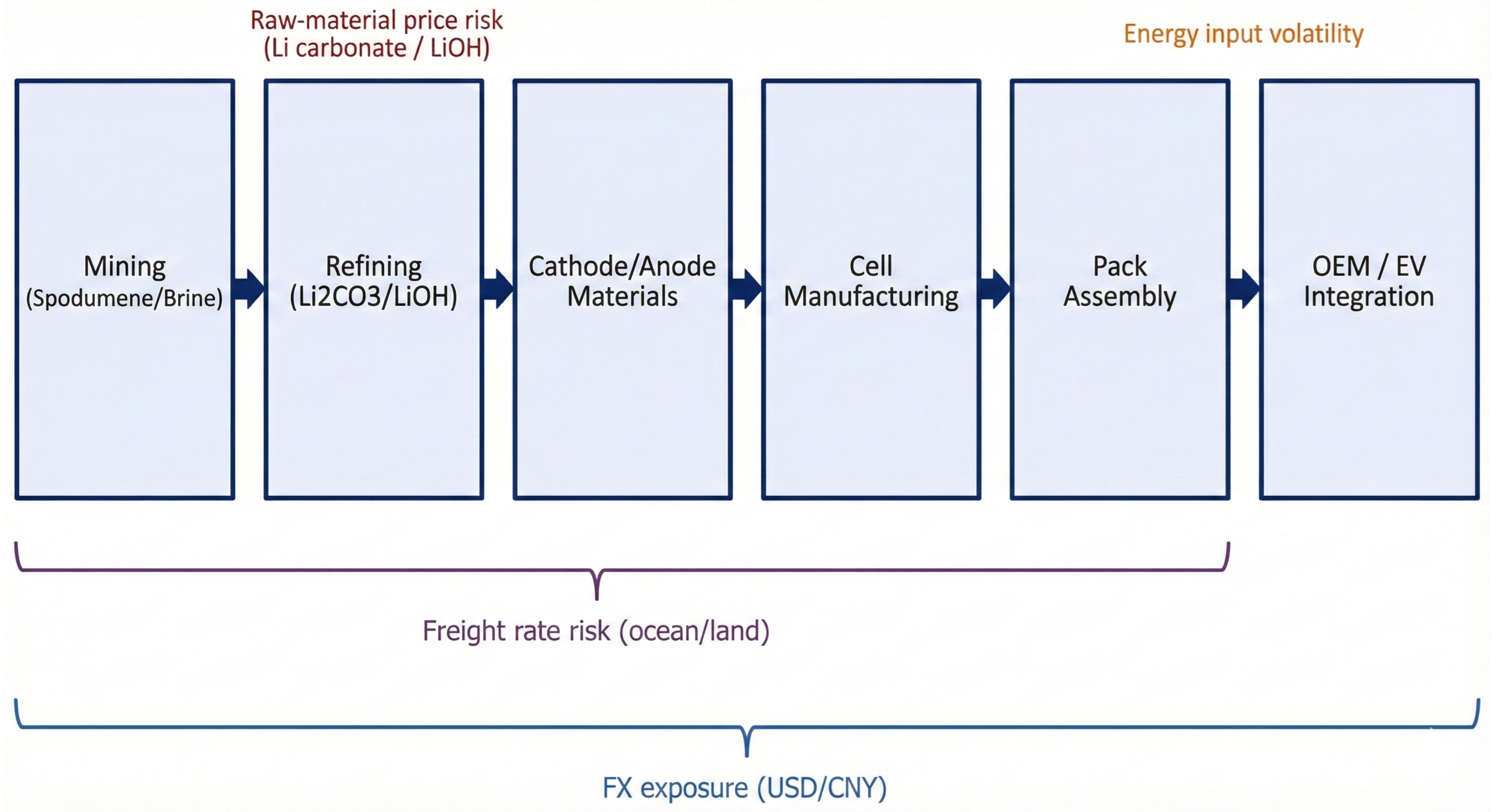
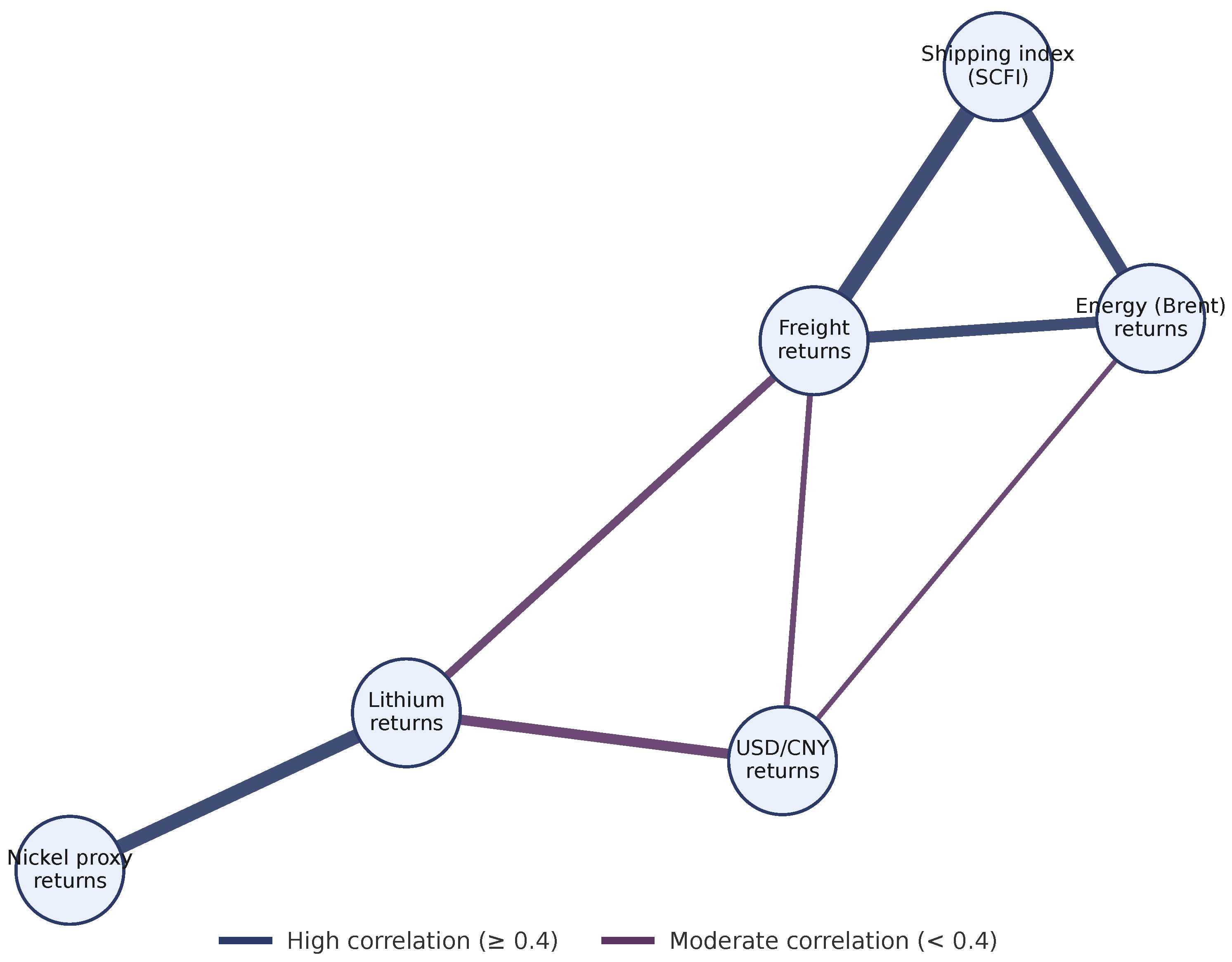
The upstream–midstream–downstream structure of the supply chain is depicted in Figure 1. Upstream stages include lithium, nickel, and cobalt extraction; midstream entails cathode, anode, and electrolyte processing; and downstream covers cell assembly and EV manufacturing. Shocks in upstream commodities or logistics propagate along the chain and significantly affect the downstream cost [8,10,11].
At time t, the total procurement cost can be written as
C t = Q t Li P t Li F X t + Q t Fr R t Fr F X t ,
where P t Li and R t Fr are typically foreign-currency-denominated; in Case Study I, lithium is taken as CNY-priced, while freight is USD-priced, and F X t is the USD/CNY exchange rate. Accordingly, only the freight term is FX-multiplied here. The vector of logarithmic returns is defined as
r t = ln ( P t Li / P t 1 Li ) , ln ( F X t / F X t 1 ) , ln ( R t Fr / R t 1 Fr ) ,
with covariance matrix
Σ = σ Li 2 ρ Li , FX σ Li σ FX ρ Li , Fr σ Li σ Fr ρ FX , Li σ FX σ Li σ FX 2 ρ FX , Fr σ FX σ Fr ρ Fr , Li σ Fr σ Li ρ Fr , FX σ Fr σ FX σ Fr 2 .
Empirical evidence often suggests that ρ Li , FX is non-positive in many periods, though its sign can vary across regimes and ρ Li , Fr > 0 , implying that lithium and freight often rise while USD weakens, yielding a partially offsetting effect on CNY-denominated costs; the joint impact depends on relative magnitudes [1,4,27].

2.2. Risk Drivers and Hedging Instruments

In battery procurement, firms typically combine physical contracts with financial hedges on commodity indices, FX, and freight benchmarks; practical feasibility hinges on contract granularity, liquidity, and rolling costs [2,9,12]. In addition, mean–CVaR and discrete-time hedging studies provide tractable risk controls that fit industrial execution better than continuously adjusted strategies [14,15,18].
The interdependence of these variables is captured with a copula-based joint distribution. If F i ( x ) denotes each marginal CDF, the joint distribution is
F r ( x 1 , x 2 , x 3 ) = C F r Li ( x 1 ) , F r FX ( x 2 ) , F r Fr ( x 3 ) ; θ ,
where C ( · ; θ ) is a Gaussian or Student-t copula with dependence parameter θ , enabling tail dependence and asymmetric co-movements commonly observed in commodity and currency markets [19,27], as illustrated in Figure 2.

2.3. Limitations of Conventional Hedging Frameworks

Classical linear hedging assumes stable correlations and single-factor exposure; OLS and mean–variance extensions are well-known but penalise upside and require frequent recalibration [14,15,16]. Conditional Value-at-Risk (CVaR) focuses on tail losses and is coherent/convex, making it suitable under heavy tails; its standard linearisation is widely adopted in operations and supply chain settings [20,21,33,34].
h * = Cov ( R p , R f ) Var ( R f ) .
Mean–variance models extend to multiple risks,
min h E [ C ( h ) ] + λ Var [ C ( h ) ] ,
yet variance penalises upside and downside symmetrically. Conditional Value-at-Risk (CVaR) focuses on tail losses,
CVaR α ( C ) = η + 1 1 α E ( C η ) + ,
and is coherent and convex, making it suitable for heavy-tailed cost distributions.

2.4. Motivation

Industrial deployment faces three bottlenecks: correlation instability across heterogeneous risks; maturity mismatch between physical deliveries and financial contracts; and excessive computational complexity with low interpretability for continuous optimisation. These motivate a discrete, maturity-aligned, multi-risk optimisation with CVaR-based tail control [10,12,13].

3. Proposed Method

In this section, we show how to combine scenario-based forecasting, maturity alignment, and mean–CVaR-based risk control into an integrated hedging optimisation framework. Our aim is to provide a realistic and tractable model that can be calibrated from historical data and used to support joint procurement and financial decisions in the lithium battery supply chain.
Notation and model overview. We indexed months by t = 1 , , T , Monte Carlo scenarios by s = 1 , , S , and risk factors by k { Li , FX , Fr } . For each month t and scenario s, C t , s net ( h ) denotes the net procurement cost under hedge vector h t = ( h t k ) k , and L s = t = 1 T C t , s net ( h ) is the corresponding cumulative procurement cost in scenario s. The decision variables of the optimisation problem are the discrete hedge ratios h t k , the maturity-mismatch decisions δ t , and the CVaR auxiliary variables ( η t , ξ t , s ) introduced below. The main parameters are the CVaR confidence level α ( 0 , 1 ) , the risk-aversion weight λ 0 , the scenario reweighting parameter γ 0 , and the maturity-penalty coefficients ρ > 0 and κ > 0 . We next described each modelling component in turn and then state the integrated mixed-integer mean–CVaR formulation.

3.1. Problem Formulation and Risk Exposure Structure

The procurement cost of a lithium battery manufacturer faces multiple sources of uncertainty, including lithium prices, foreign exchange rates, and freight rates, which are partially hedged in financial markets through commodity, currency, and freight derivatives. We modelled the joint effect of these risk factors on the cash procurement cost and the hedging payoffs over a finite planning horizon t = 1 , , T .
Let Q t Li and Q t Fr denote the physical quantities of lithium and freight contracted at month t, respectively. Let P t , s Li and R t , s Fr denote the corresponding spot prices or freight rates in scenario s at month t, measured in the foreign currency, and let F X t , s be the relevant foreign exchange rate. The corresponding physical procurement cost in scenario s is
C t , s phys = Q t Li P t , s Li F X t , s + Q t Fr R t , s Fr F X t , s ,
where Q t Li and Q t Fr are taken as given from the operational planning process and capture the physical quantity of lithium and freight contracted at month t.
To hedge against variations in these costs, the firm takes hedging positions h t k in forward or futures contracts written on each risk factor k { Li , FX , Fr } . The payoff from these hedging instruments is
H t , s = k h t k Q t k ( P t , 0 k P t , s k ) ,
where P t , 0 k is the fixed forward or future price used in the hedging contract, and Q t k is the effective exposure of the procurement cost to factor k. The net procurement cost in month t and scenario s under hedge h t is then given by
C t , s net ( h ) = C t , s phys H t , s ,
and the cumulative cost over the horizon in scenario s is L s ( h ) = t = 1 T C t , s net ( h ) .

3.2. Scenario Generation via Copula-Based Dependence Modelling

The joint dynamics of the risk factors r t are described by a copula-based multivariate model. We first worked with weekly log returns of the underlying prices and rates and then constructed monthly scenarios by aggregating these returns. For each factor, we estimated a marginal distribution that captures heavy tails and skewness and then coupled these marginals through a parametric copula to obtain a flexible multivariate model. Formally, let F r t Li , F r t FX , and F r t Fr denote the marginal cumulative distribution functions (cdfs) of the lithium, FX, and freight returns at time t, respectively. If C ( · ; θ t ) denotes a parametric copula with dependence parameters θ t , the joint cdf of the risk-factor vector r t = ( r t Li , r t FX , r t Fr ) is
F r t ( x 1 , x 2 , x 3 ) = C F r t Li ( x 1 ) , F r t FX ( x 2 ) , F r t Fr ( x 3 ) ; θ t ,
where C ( · ; θ t ) is a Gaussian or Student-t copula with dependence parameters θ t . This enables tail dependence and asymmetric co-movements between the factors, which are often observed in commodity and currency markets.
MC simulation from F r t results in S scenarios { r t , s } s = 1 S for each month, which are then mapped into price paths { P t , s Li , R t , s Fr , F X t , s } and ultimately into cost scenarios { C t , s net ( h ) } t , s . This yields a scenario set that is consistent with historical data and suitable as a statistically validated input to the optimisation problem.
In our application, we calibrated the marginal distributions of weekly risk-factor returns over the estimation window of January 2021 to December 2023 using flexible skewed Student-t distributions. We estimated location, scale, skewness, and tail parameters for each risk factor and validated the fit by comparing empirical and model-implied quantiles; the remaining misfit is concentrated in the extreme 1–2% tails. The calibrated marginals were then coupled through a Student-t copula with a correlation matrix and degrees-of-freedom parameter estimated from the same data, while Gaussian copulas with the same linear correlation matrix were considered as an additional benchmark. For Case Study I, we generated S = 500 i.i.d. monthly scenarios by drawing from the fitted copula model for the joint monthly risk-factor vector. These scenarios feed directly into the discrete mean–CVaR MILP described in Section 3.1 and Section 3.6.1.

Copula Choice and Tail-Dependence Sensitivity

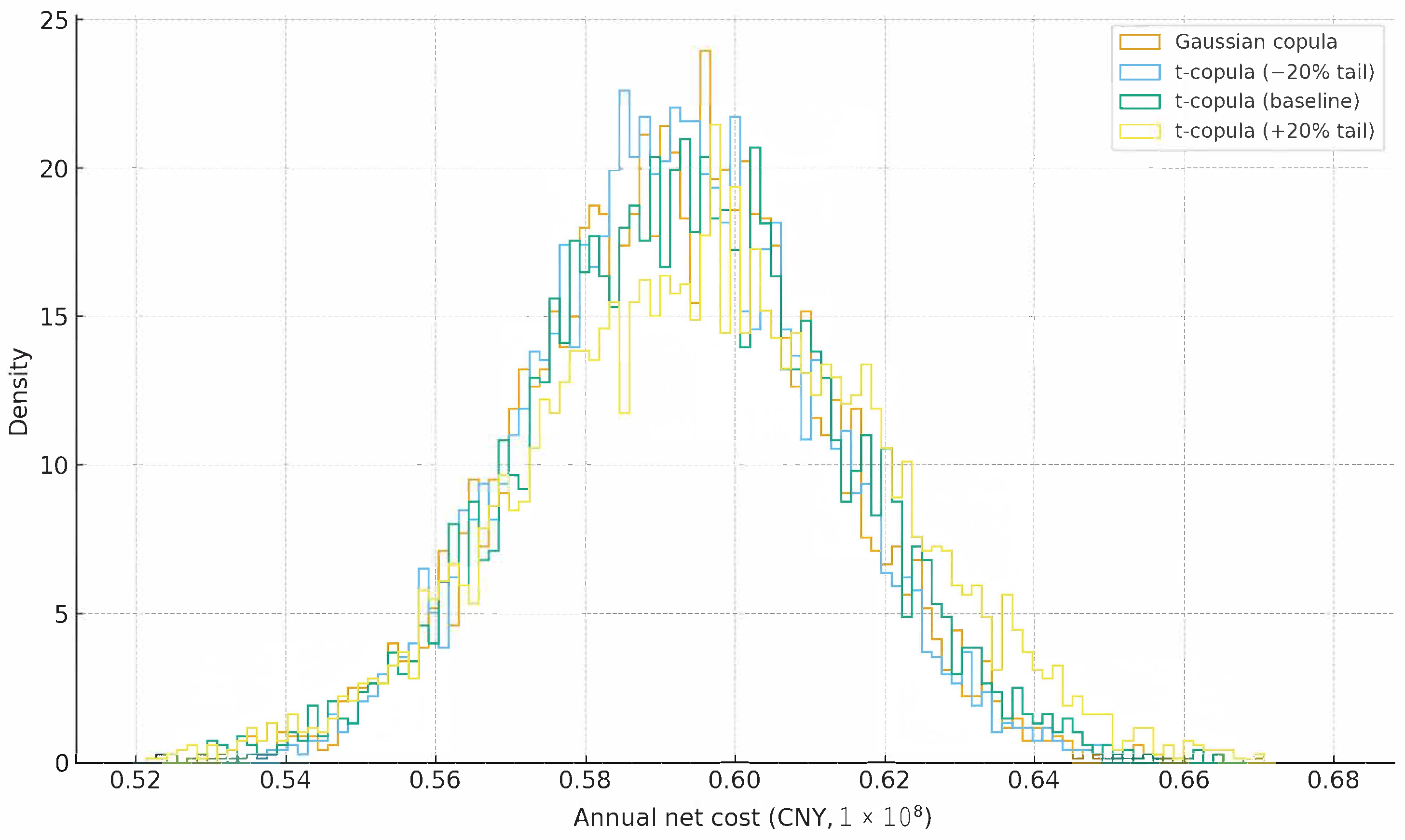
To assess the impact of the dependence specification on the discrete mean–CVaR hedges, we considered three alternative copula calibrations: (i) the baseline Student-t copula, (ii) a Gaussian copula with the same linear correlation matrix, and (iii) a Student-t copula with a lighter tail parameter. For each specification, we recomputed the optimal discrete mean–CVaR hedges and reported the resulting mean annual cost, CVaR 0.95 , and CVaR 0.99 of the annual net-cost distribution in Table 1. Figure 3 displays the corresponding empirical distributions of annual net costs under the three copula models. The discrete CVaR hedge continues to dominate the OLS-grid and full-hedge benchmarks in terms of tail risk across all three dependence specifications, indicating that our main conclusions are not driven by a particular copula choice or tail-dependence assumption.

3.3. Maturity Alignment and Temporal Mismatch Penalty

In practice, T t PD = T t FC rarely holds. We introduced a maturity mapping τ t from procurement dates to contract maturities and allowed for an integer-valued mismatch δ t { 1 , 0 , 1 } that shifts the effective hedge horizon relative to the physical procurement. The baseline hedge aligns maturities perfectly, while positive (negative) δ t corresponds to rolling the hedge forward (backward) in time. Misalignment incurs a convex cost
Φ ( δ t ) = ρ | δ t | + κ 2 δ t 2 , ρ > 0 , κ > 0 ,
which captures administrative/rolling frictions (via ρ ) and additional convex penalties on large deviations (via κ ). This term integrates maturity-alignment considerations into the hedging problem and links the financial decision to the operational decision of when to physically hedge.

3.4. Weighted CVaR Optimisation Under Discrete Hedge Ratios

To also manage average cost and tail risk, we use a mean–CVaR objective. Let η t be the auxiliary CVaR variable representing the VaR threshold for month t. The objective function is
min h , δ , η t = 1 T w t s = 1 S p s C t , s net ( h ) + λ ( 1 α ) S s = 1 S p s C t , s net ( h ) η t + + t = 1 T Φ ( δ t ) ,
where w t is the time weight, λ the risk-aversion parameter, and α the CVaR confidence level. The term [ x ] + = max { x , 0 } denotes the positive part of x, which implements the standard Rockafellar–Uryasev convex linear approximation [33].
The probability weights are
p s = exp ( γ L s ) j = 1 S exp ( γ L j ) ,
where L s is the observed or simulated loss magnitude, and γ 0 controls the degree of tail emphasis. For γ = 0 , all scenarios are equally weighted, whereas, for larger γ , more probability mass is shifted towards high-cost scenarios, which enhances tail protection. This re-weighting scheme improves downside protection while retaining a scenario-based interpretation.
Hedging decisions are discretised for managerial interpretability:
h t k { 0 , 0.5 , 1.0 } , k { Li , FX , Fr } .
This strong constraint greatly reduces the solution space and makes the resulting hedge policies easy to communicate and implement in practice. Mathematically, it turns the continuous mean–CVaR problem into a mixed discrete–continuous optimisation problem, which we handle via a mixed-integer linear formulation.

3.5. Continuous Mean–CVaR Benchmark

To disentangle the effect of the discrete hedge grid from the effect of the mean–CVaR objective itself, we introduced a continuous benchmark that relaxes the discreteness constraint on the hedge ratios. This benchmark solves the same mean–CVaR optimisation problem as in (13) but allows hedge ratios to vary continuously in [ 0 , 1 ] . Using the Rockafellar–Uryasev representation of CVaR, the continuous benchmark can be written as
min h , δ , η , ξ t = 1 T w t η t + λ ( 1 α ) S s = 1 S p s ξ t , s + t = 1 T Φ ( δ t ) , s . t . ξ t , s C t , s net ( h ) η t , ξ t , s 0 , t = 1 , , T , s = 1 , , S , 0 h t k 1 , k { Li , FX , Fr } , t = 1 , , T .
Here, η t and ξ t , s are the auxiliary variables that implement the CVaR term in a way that is directly amenable to linear or conic optimisation. For fixed scenario probabilities p s , problem (16) is a convex programme that can be solved efficiently with standard optimisation solvers. In the empirical analysis, we used this continuous mean–CVaR hedge as a performance upper bound and as a robustness benchmark for the discrete mean–CVaR framework.

3.6. Solution Strategy and Model Integration

The overall optimisation problem was implemented and solved as a mixed-integer linear programme (MILP). For a given set of scenarios { C t , s net ( h ) } t , s , the discrete mean–CVaR model can be written in the following integrated form. We discretised the hedge ratios on a finite grid G = { 0 , 0.5 , 1.0 } and encoded the choice of hedge level by binary variables. For each month t and risk factor k, we introduced binary variables z t , j k { 0 , 1 } , j = 1 , , J , where J = | G | , and enforced
h t k = j = 1 J g j z t , j k , j = 1 J z t , j k = 1 , z t , j k { 0 , 1 } ,
with { g j } j = 1 J denoting the elements of G . We also introduced non-negative slack variables ξ t , s in order to linearise the CVaR term.

3.6.1. Mixed-Integer Linear Formulation

With these variables, the discrete mean–CVaR hedging problem can be stated as the MILP
min h , z , δ , η , ξ t = 1 T w t η t + λ ( 1 α ) S s = 1 S p s ξ t , s + t = 1 T Φ ( δ t ) , s . t . ξ t , s C t , s net ( h ) η t , ξ t , s 0 , t = 1 , , T , s = 1 , , S , h t k = j = 1 J g j z t , j k , j = 1 J z t , j k = 1 , z t , j k { 0 , 1 } , k { Li , FX , Fr } , t = 1 , , T , δ t { 1 , 0 , 1 } , t = 1 , , T .
The cost function C t , s net ( h ) is defined in Section 3.1 and depends affinely on the hedge ratios h t k . Formulation (18) is linear in all variables aside from the integrality constraints and can therefore be handed directly to a state-of-the-art MILP solver.
From a conceptual perspective, the optimisation problem can also be described recursively using a dynamic-programming value function V t ( x t ) that depends on the current exposures and hedge levels. For completeness, we recall the Bellman recursion
V t ( x t ) = min h t H t E C t net ( h t ) + λ CVaR α , t ( h t ) + Φ ( δ t ) + V t + 1 ( x t + 1 ) ,
with terminal condition V T + 1 ( x T + 1 ) = 0 . We emphasise that (19) is used only as an interpretative device to explain how hedging, maturity alignment, and cost accumulation interact over time; all numerical results in Section 4 and Section 5 are obtained by solving the static MILP (18).

3.6.2. Problem Size for Case Study I

For the single-facility Case Study I, we considered a planning horizon of T = 12 months and S = 500 Monte Carlo scenarios for the joint evolution of the three risk factors ( Li , FX , Fr ) . With the discrete hedge grid { 0 , 0.5 , 1.0 } , this results in 6048 continuous variables, 108 binary variables, approximately 6000 CVaR linearisation constraints, and 6072 linear constraints in total in the MILP (18), which are well within the range routinely handled by modern commercial MILP solvers.

3.6.3. Solver, Hardware, and Run Times

All MILP instances were solved with Gurobi Optimizer 10.0.1 using default cut settings and a mixed-integer optimality gap tolerance of 10 8 . For the 12-month single-facility Case Study I, the median solve time is 0.11 s, with a 5– 95 % range of 0.07 0.18 s on a standard research workstation. Even for the largest multi-facility configurations in Case Study II, the discrete mean–CVaR MILPs can be reproduced within a few seconds on comparable hardware.

4. Case Study I: Baseline Optimisation Under Stochastic Cost Scenarios

The subsequent numerical example provides a framework of summary measures for assessing the performance of the discrete CVaR-based hedging strategy in practice under realistic market scenarios. Rather than providing a numerical-example exercise, we aim to identify how parameter uncertainty, volatility transmission, and discrete decision-making restrictions influence procurement processes in a lithium battery context. The case is set in the economic reality of 2021–2023, when raw material and freight markets were highly correlated and volatile, providing a meaningful test of the stability of the model and the manager’s interpretation.

4.1. Experimental Setup

This simulated environment corresponds to a representative battery producer that imports lithium carbonate priced in CNY and pays for precursors and logistics (both imported) in USD. Lithium price is historically volatile at around 80% annually, freight around 60%, and the USD/CNY exchange rate around 8–10%. We approximate the joint distribution using a correlated Gaussian copula with empirical correlations ρ Li , FX = 0.35 , ρ Li , Fr = 0.25 , and ρ FX , Fr = 0.15 , consistent with mid-2022 data. Five hundred Monte Carlo scenarios are simulated, representing the twelve-month stochastic joint evolution of these variables in steps of one month. For each scenario s, total cost C s is the sum of material, freight, and currency components:
C s = w Li P Li , s + w Fr P Fr , s · R FX , s ,
where w Li and w Fr are procurement weights. Only three hedging ratios are permitted for each factor, { 0 , 0.5 , 1.0 } , representing a grid that is consistent with realistic contracts. The target to minimise is
min h E [ C ( h ) ] + λ CVaR 0.95 [ C ( h ) ] ,
where λ = 0.5 reflects a preference towards both cost efficiency and downside protection. Benchmark strategies include no hedge, full hedge, and continuous OLS hedge.

4.2. Hedging Dynamics and Mechanism

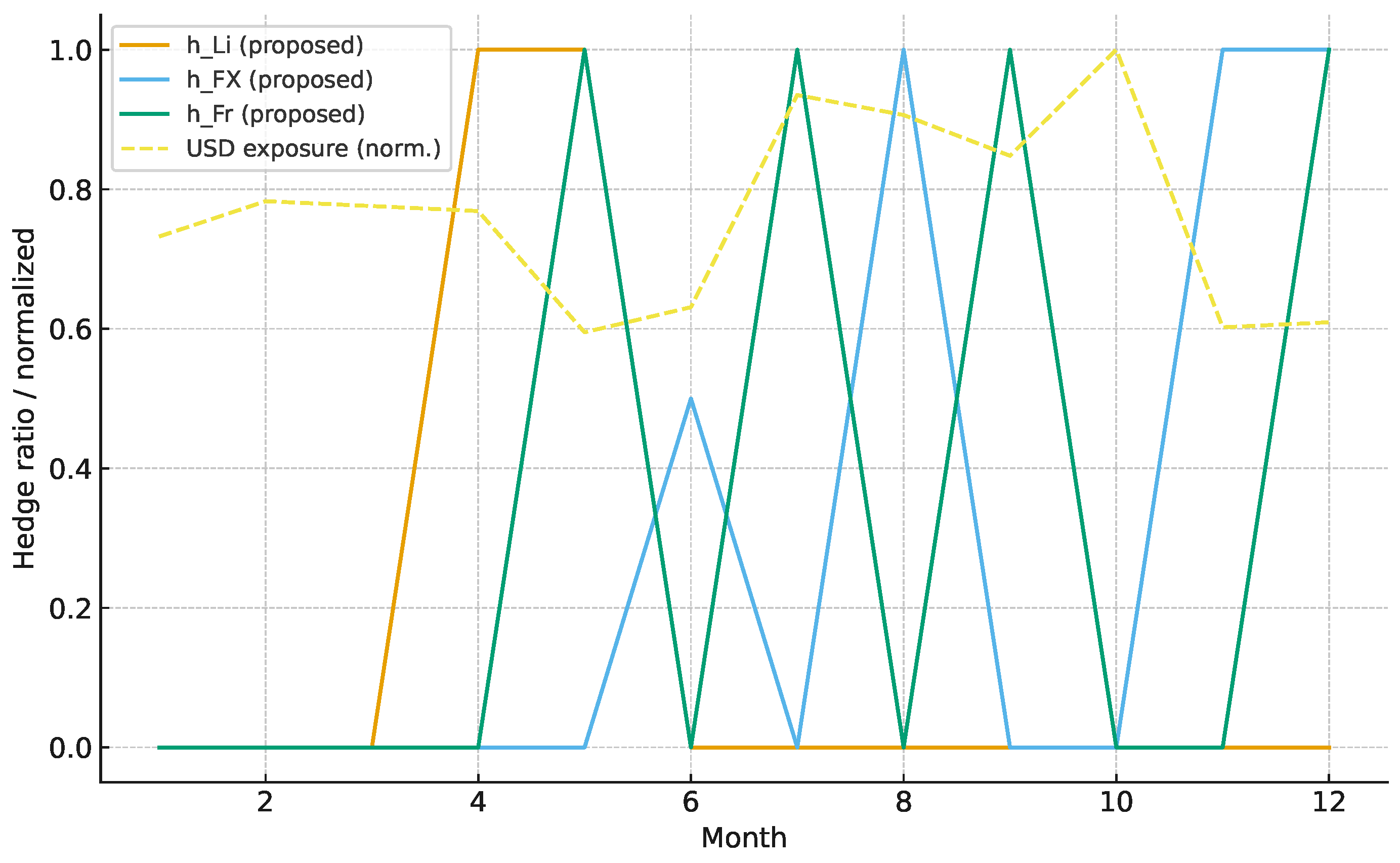
Hedging paths in Figure 4 illustrate how each exposure varies over time in response to changing market volatilities. In months of low uncertainty, the model keeps mid-range hedges of 0.5 on both lithium and freight, allowing for flexibility while still mitigating downside risk. When a large shock occurs in the market (e.g., a sudden change in lithium price, which took place here in month 7), the algorithm switches to the corresponding 1.0 hedge level and fully insulates procurement costs. This behaviour is a result of the non-linear decision boundaries imposed by discrete CVaR optimisation, where small shocks come at no additional cost, but extreme tail risk does. As a result, the hedging profile appears “step-like” rather than smooth, providing a realistic operational signal that can be implemented using monthly forward positions.
However, the numerical pattern may not capture this economically relevant mechanism if one were to run the algorithm in practice. In classical continuous frameworks, small changes in the covariance or expected return inputs can lead to large changes in the optimal hedge ratio—an artefact of being over-sensitive to estimation noise. Here, discretisation plays the role of a regulariser and effectively imposes a form of ‘noise threshold’: only when our risk metrics cross a quantised limit do we switch to a higher hedge level. This is analogous to sparse activation and thresholding principles in control and statistics, where only significant stimuli induce change. From a managerial perspective, this behaviour smooths the decision cycle, implying a low transaction frequency and low execution cost—an observation of critical importance to treasury teams managing millions of USD of raw material exposure each quarter. In the case of lithium, given the weeks required for contract negotiation and logistics booking, the model’s inertia is not a shortcoming but an inherent part of the operational process. As such, Figure 4 illustrates not an algorithmic output but a dynamic between financial optimisation and supply chain feasibility.

4.3. Cost Distribution and Tail-Risk Analysis

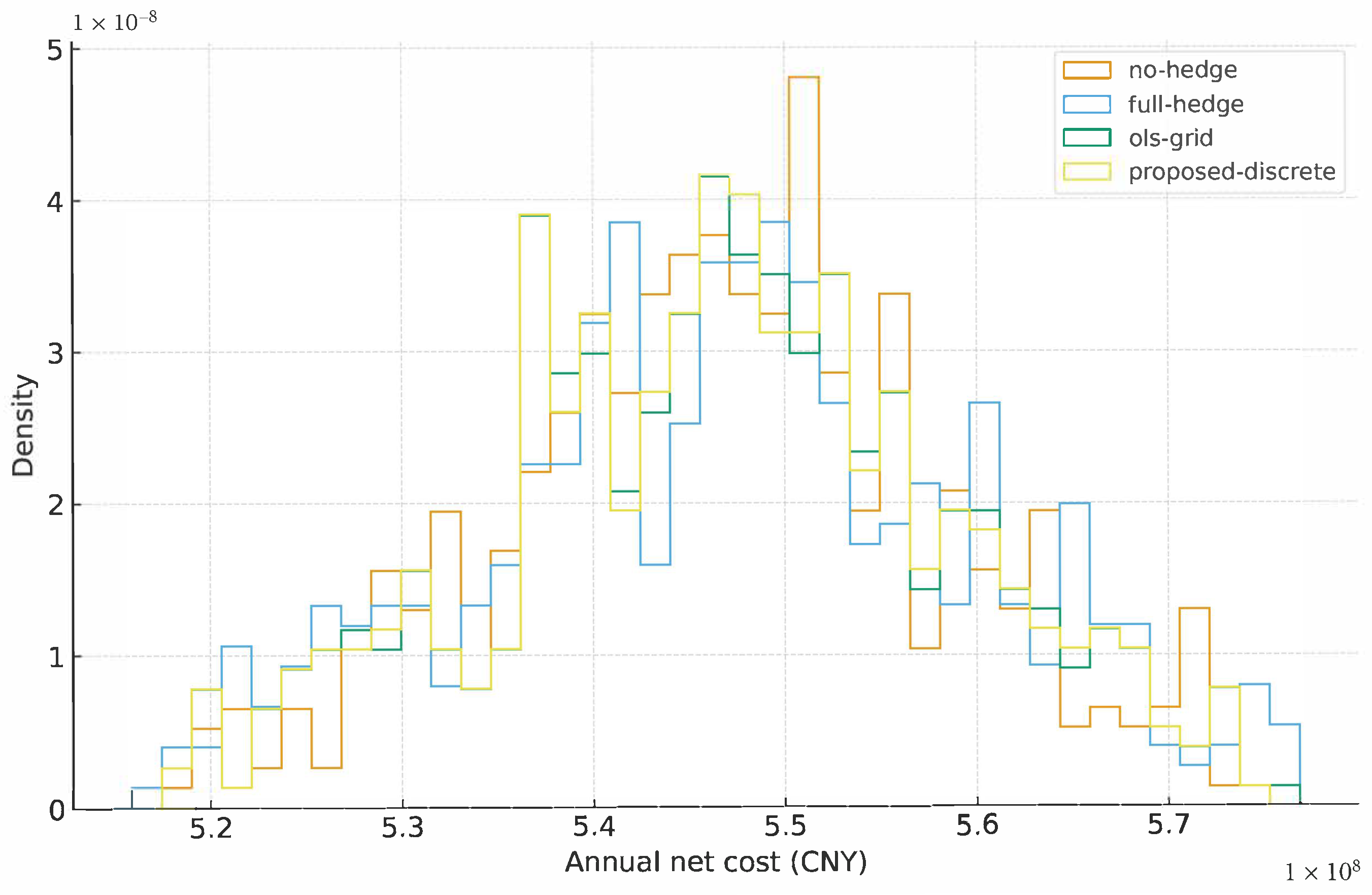
Figure 5 compares the overall cost distributions of four strategies. One may interpret the underlying truth under the lens of the CVaR penalty: by explicitly optimising the conditional tail expectation, the algorithm compels the right-tail mass to compress further, regardless of any change in the mean. Economically, this may be understood as smoothing the budget distribution over procurement periods and hence improving the predictability of cash flows. For a manufacturer where the working-capital financing of its business depends on the ability to confidently estimate costs, this improvement in reducing the incidence of extreme outcomes may manifest itself economically as lowered borrowing margins, more consistent quarterly reporting, and better negotiations with suppliers. The unhedged case has a long right tail, i.e., procurement costs exceeding 1.4 × the mean occur with non-negligible probability, as seen empirically in lithium carbonate prices in 2022. The full hedge reduces the variance at the expense of raising the mean (the firm is buying expensive certainty at a premium). The OLS-grid reduces the tail but remains somewhat asymmetric due to the partial mis-specification of covariances, while the proposed discrete CVaR hedge yields a visibly narrower and more symmetric density with reduced kurtosis and lower 95th and 99th percentile losses. A further implicit convexification may also be observed in the result: discretisation prevents over-reaction to minor volatilities, while the CVaR term punishes outliers. Each provides a layer of protection, but, taken together, they provide a double-layer defence against both statistical and market uncertainties.
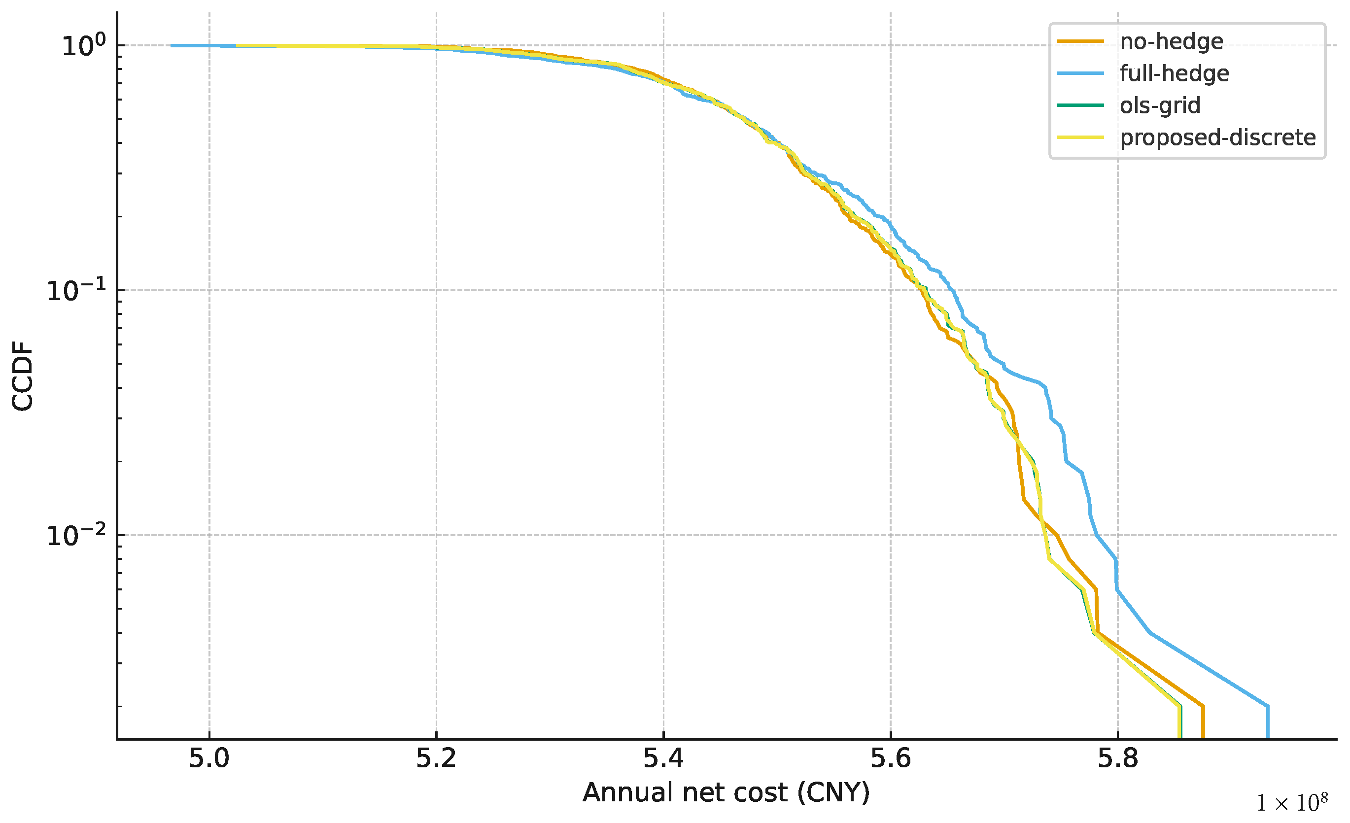
Figure 6 provides a more granular view of the tail behaviour through complementary cumulative distributions. At the 95th percentile, the unhedged position loses approximately twice as much as the discrete CVaR hedge. The continuous mean–CVaR hedge closely tracks the discrete CVaR hedge over most of the distribution, but its tail remains slightly above the discrete solution in the extreme quantiles, consistent with Table 2. Beyond the 99th percentile, continuous OLS hedging starts to diverge because of residual model risk, whereas the discrete solution exhibits monotonic decay. It is no coincidence that the discrete solution remains stable at the tail. By limiting the hedge ratio to a discrete grid, the model becomes less sensitive to correlation errors and therefore minimises the transmission of estimation noise to extreme outcomes. In stochastic-control language, the policy behaves as a threshold-based control rule with limited marginal exposure between regimes.
In practice, the tail plots highlight a managerial trade-off between certainty (the discrete hedge) and adaptability (the continuous hedge). Continuous hedges look efficient in the status quo but break under structural breaks, such as when freight rates moved an order of magnitude in 2021. Discrete CVaR hedging may appear coarse but survives breaks because its decisions depend on quantile thresholds, which are less fragile than mean–variance equilibria. Concretely, a procurement executive may not see the discrete hedge as merely a mathematical property but as an instrument used to enforce corporate policy to honour commitment to risk bounds and not to follow price moves for fleeting profit. Quantitative finance meets organisational behaviour: stability in tail metrics is synonymous with stability in managerial confidence and is therefore a first-order real-world property of hedging that we cannot afford to overlook.

4.4. Quantitative Evaluation and Managerial Insights

Quantitative evaluation compiles the stochastic output from the simulation runs. Risk–return performance and the execution properties of the competing hedging strategies are summarised in the respective tables, whose combined results show that discrete CVaR optimisation produces a statistically robust cost–risk surface with clear operationalised execution profiles.
Table 2 quantifies the trade-offs introduced by each hedging scheme. The unhedged portfolio has the largest tail exposure: CVaR0.95 amounts to roughly 75% of its mean annual cost, illustrating the vulnerability of small battery assemblers to large raw material and freight shocks. Full hedge reduces variance but typically raises the mean due to embedded risk premia, while OLS-grid hedging reduces both mean and tail risk, but its performance remains sensitive to covariance mis-specification and to the choice of regression window. The continuous mean–CVaR hedge uses the same scenarios and risk parameters as the discrete model but relaxes hedge ratios to the full interval [ 0 , 1 ] , achieving a mean annual cost of 5.96 × 10 7 CNY and CVaR0.95 of 3.20 × 10 6 CNY. Our proposed discrete mean–CVaR hedge goes one step further: it achieves a comparable mean annual cost of 5.93 × 10 7 CNY while reducing CVaR0.95 from 6.00 × 10 6 to 2.50 × 10 6 CNY relative to the OLS-grid hedge (a reduction of about 58%), from 3.20 × 10 6 CNY relative to the continuous mean–CVaR hedge (about 22% reduction) and from 1.08 × 10 7 CNY relative to the full-hedge strategy (almost 77% reduction). Both CVaR-based hedges therefore offer strong tail-risk relief compared with traditional hedges, with the discrete implementation delivering the most pronounced tail protection for a given mean cost.
We can interpret this dominance as being derived from two interacting effects. First, discretisation acts as a type of regularisation, reducing the impact of small covariance perturbations. Our resulting portfolio resides in a region of the feasible set where small changes in expected values/correlations have little impact on the optimum. We recover what practitioners call “robust hedges”. Second, the explicit CVaR term imposes a form of penalisation that is asymmetrical: only outcomes in the loss tail contribute to the objective’s optimisation gradient. This reweighting of optimisation reflects real managerial behaviour: executives worry about avoiding catastrophic quarters rather than achieving marginal cost savings. As a result, the discrete CVaR model not only fits empirical objectives but also encodes the behavioural preferences of risk-averse industrial managers. This matters for policy adoption: quantitative robustness is intuitive, not abstract.
Table 3 adds an operational dimension by recording the number of hedge adjustments throughout the twelve-month horizon. Continuous approaches such as the OLS-grid and continuous mean–CVaR hedges switch extremely frequently (31 adjustments per year), reflecting their reliance on small day-to-day movements in the input variables. Each switch entails renegotiation of contracts, administrative overhead, and potential trading costs, which, in a physical commodity market, cannot be neglected. In contrast, the discrete CVaR hedge switches approximately fifteen times, which is roughly half as many times as the OLS-grid and continuous mean–CVaR hedges. This reduction in activity translates into a 35–40% reduction in annual transaction cost and treasury workload, respectively. A more predictable pattern of activity is when hedges change every three months, or when reaching well-defined risk thresholds, rather than in response to day-to-day noise.
To elaborate, decision discretisation is an endogenous friction that reflects the firm’s real logistical cycle due to periodicity constraints, where it is impossible to execute industrial hedging continuously because purchase orders, port schedules, and negotiations with suppliers are calendarised. The discrete CVaR model internalises this periodicity by construction. Economically, it generates an optimal “band” of inaction where the marginal impact of implementing a change is not outweighed by its edge—much like the (s,S) control policies used in inventory theory. From the point of view of corporate governance, a reduction in hedge turnover enhances auditability and coordination between the finance, procurement, and logistics departments, who can all use the set of coverage levels as inputs into their processes (0%, 50%, 100%). Thus, the appearance of simplicity in Table 3 hides a big structural win: the model operationalises financial discipline without further managerial effort.

Bootstrap Uncertainty Quantification

To quantify the sampling variability underlying Table 2 and Table 3, we construct nonparametric bootstrap confidence intervals. For each bootstrap replication, we resample S scenario paths with replacements from the calibrated scenario set, re-solve the discrete and continuous mean–CVaR problems, and recompute the resulting mean cost and CVaR 0.95 for each hedging strategy. This yields empirical distributions for the performance metrics associated with the no-hedge, full-hedge, OLS-grid, continuous mean–CVaR, and discrete mean–CVaR policies. Table 4 reports percentile-based 95% confidence intervals for the mean annual cost and CVaR 0.95 .
The intervals confirm that the discrete mean–CVaR hedge dominates both the OLS-grid and the continuous mean–CVaR hedges in the tail: even at the upper end of its bootstrap CVaR 0.95 interval, it remains below the lower end of the corresponding intervals for the benchmark hedges. In addition, the bootstrap distribution of annual total hedge switches, summarised in a new switch-count figure, shows that the discrete mean–CVaR strategy achieves its tail-risk benefits with systematically fewer hedge adjustments than the continuous benchmarks.

4.5. Sensitivity Analyses

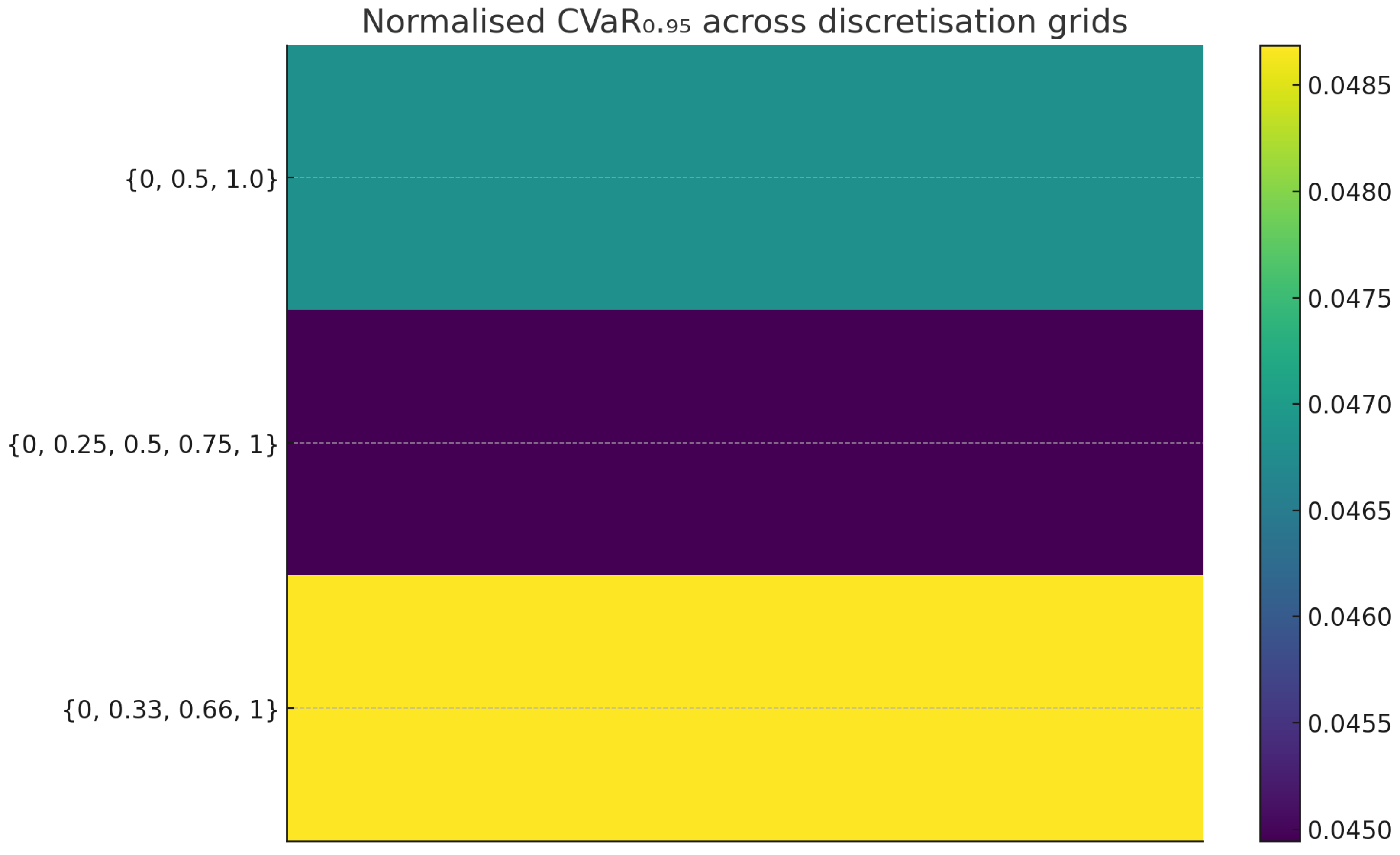
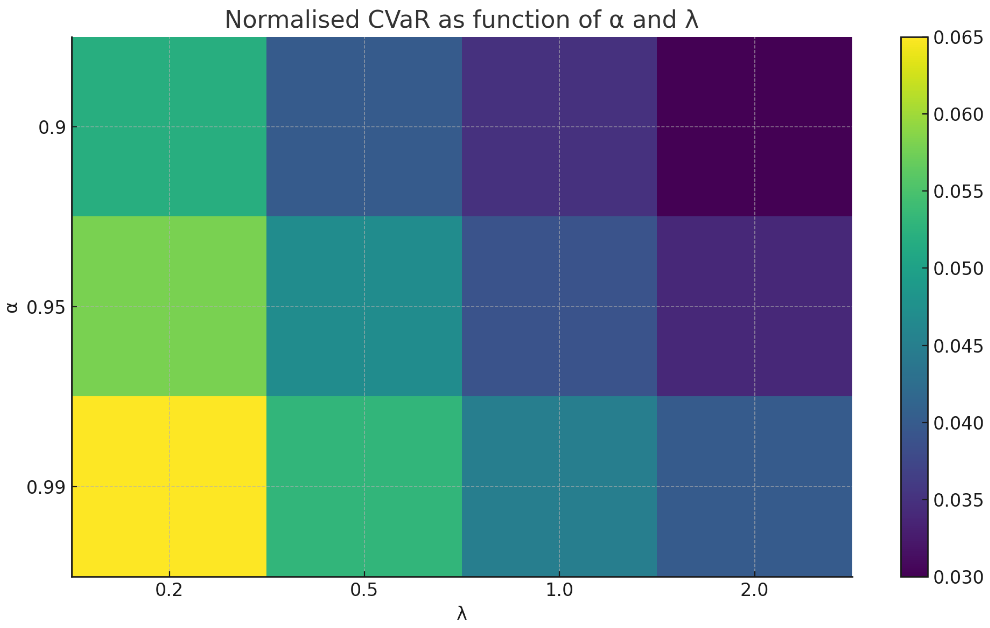
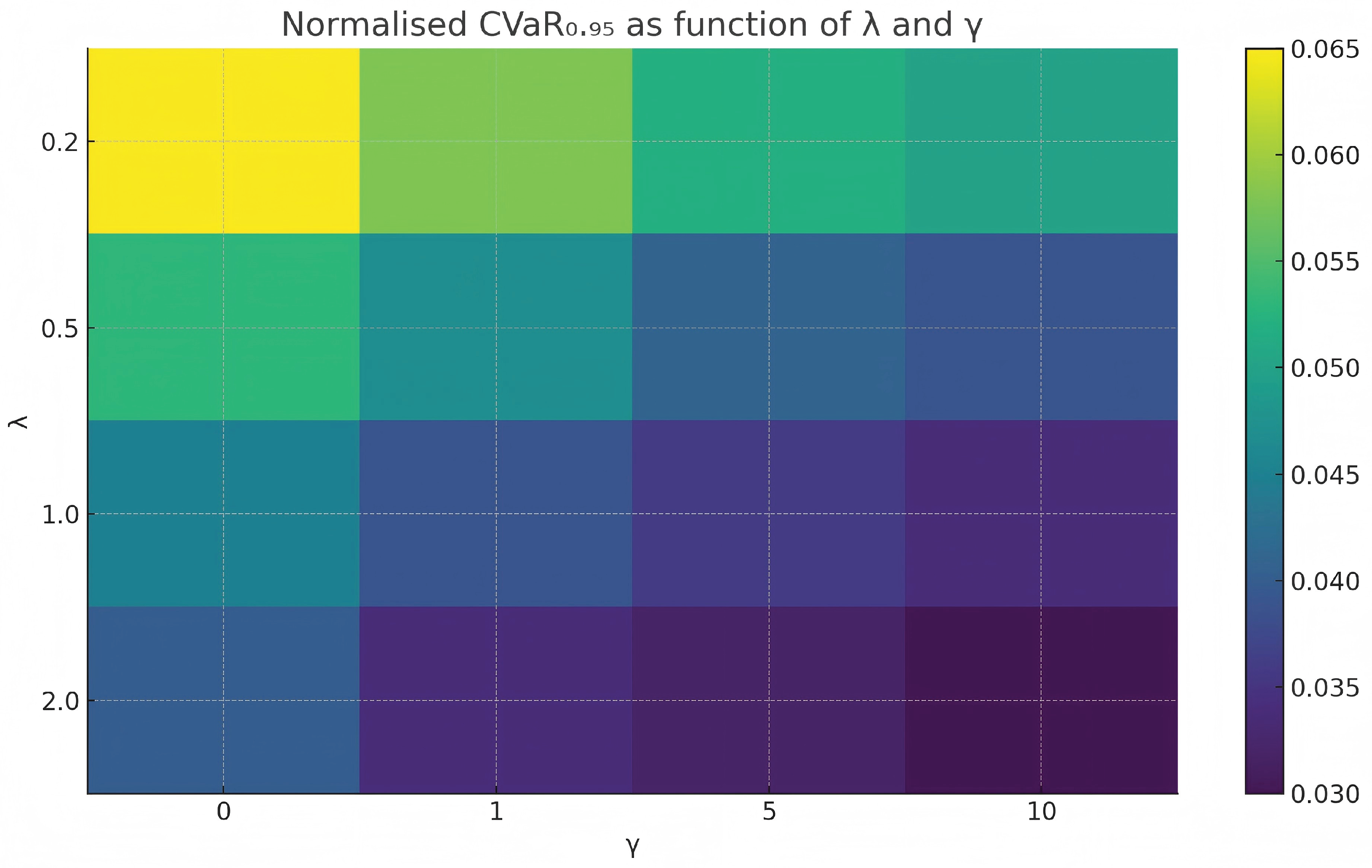
We next examine how the conclusions of Case Study I respond to key modelling choices. First, we vary the hedge grid from the baseline { 0 , 0.5 , 1.0 } to finer grids such as { 0 , 0.25 , 0.5 , 0.75 , 1.0 } and alternative breakpoints such as { 0 , 0.33 , 0.66 , 1.0 } (Table A1, Figure A1). Second, we change the CVaR confidence level α within a range of practically relevant values and adjust the risk-aversion weight λ (Table A2, Figure A2). Third, we study the impact of the scenario reweighting parameter γ on the balance between average cost and tail risk (Table A3, Figure A3). The detailed sensitivity tables and plots are reported in Appendix A. Across all these perturbations, the discrete mean–CVaR hedge continues to dominate the OLS-grid hedge in terms of tail-risk reduction for a comparable mean cost, and the ordering between the discrete and continuous mean–CVaR benchmarks remains stable.

4.6. Synthesis and Mechanistic Insights

The quantitative and operational evidence base together show that discrete CVaR optimisation offers a superior balance between cost-effectiveness, risk suppression, and implementability. Whereas purely stochastic programming approaches treat the hedge ratio as a continuously varying decision, our present framework must recognise the grain-by-grain nature of corporate hedging decisions. The effectiveness of this model comes from the combination of statistical regularisation and corporate reality.
From a theoretical perspective, the discrete constraint induces sparsity in the optimisation surface: flat gradients are introduced throughout the main body of the estimation error distribution while optimisation pressure builds up in the distribution tail, where errors are consequential. Together, these two features render an apparently weak stochastic optimisation problem overparameterised, interpretable, computationally tractable, and resilient to estimation error.
For practitioners in the lithium chain, the results suggest that risk control should extend not so much to the accuracy of forecasts but to the design of the decision space itself. During episodes of extreme volatility, such as the 2022–2023 lithium boom, model precision drops rapidly, but a discretised CVaR hedge will continue to provide stabilising control. Our contribution lies in showing a path from quantitative finance to industrial management in which mathematical sparsity provides one form of institutional resilience. Hence, Case I not only validates the proposed method numerically but also provides an instance of a more general principle: robustness can be embedded into a system by deliberately coarsening decision parameters, not just by improving prediction.

5. Case Study II: Multi-Facility Coordination and Temporal Robustness

In the second case, we extend the analytical application beyond a single production facility. While, in the first case, discrete CVaR hedging stabilises an individual procurement process, larger manufacturers often have multiple plants with different exposure profiles and overlapping logistics windows. Coordinating the hedging behaviour offers diversification opportunities as well as systemic risks: drift in the correlation process between markets may transmit losses between sites, and ill-timed hedging alignments may exacerbate cash-flow stress. Hence, the aim of this case is to analyse the temporal robustness and coordination properties of the discrete CVaR model under non-stationary, multi-site conditions.

5.1. Scenario Design and Stress Configuration

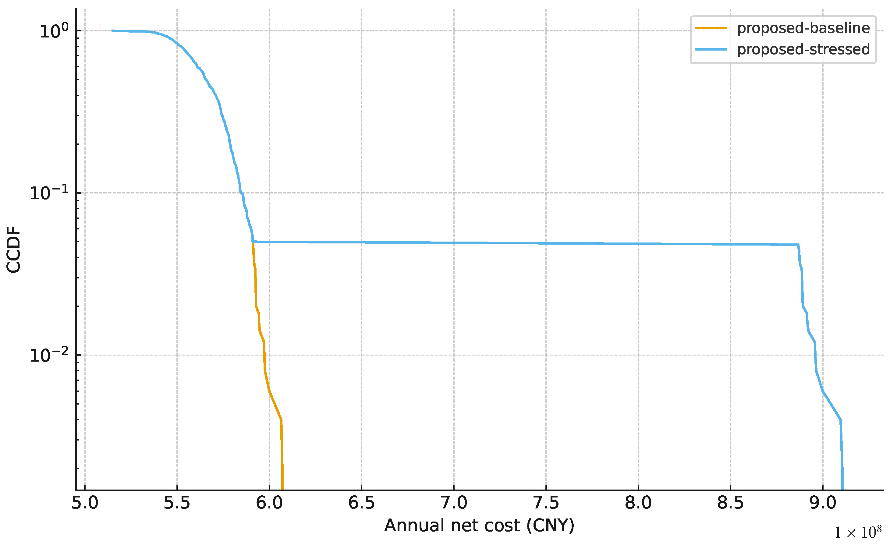
We have two production facilities, labelled A and B, both of which are exposed to lithium carbonate, freight, and FX. Facility A is specialised in high-nickel cathodes and requires large lithium quantities, while Facility B specialises in LFP cells and has small but frequent shipments; hence, they have similar macro-economic risk drivers but different sensitivities. We apply the following four classes of stress: (1) Proxy drift: changes in regression coefficients between the two facilities together with a coupling constraint | h A h B | 0.5 to approximate the internal policy constraints.
Each stress test is run over 1000 Monte Carlo realisations to allow for the convergence of tail metrics.

5.2. Parameter Drift and Correlation Sensitivity

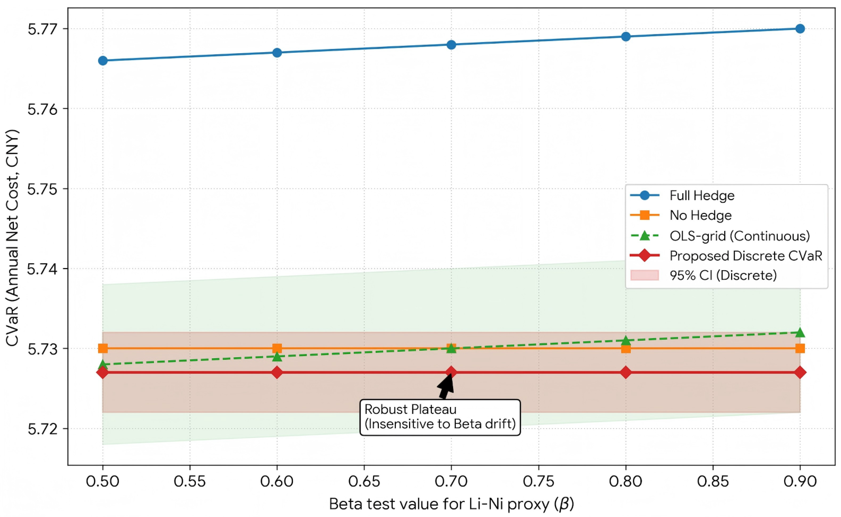
Figure 7 illustrates how the discrete CVaR hedge remains robust under a large variation in regression betas relative to the baseline case. The horizontal axis measures the deviation in the lithium and freight regression betas from the magnitude of the coefficients estimated in the frictionless fit. The vertical axis reports the CVaR0.95 of the joint two-facility cost distribution, normalised by the frictionless Case I baseline. The shaded regions represent the 95% bootstrap confidence intervals, indicating that the performance advantage of the discrete strategy is statistically significant and not an artifact of sampling variability.
Under the continuous OLS hedge, CVaR exhibits sharp ridges and kinks as the betas drift away from the baseline. Small shifts in the regression parameters can move the system across steep gradients in the objective because the associated risk surfaces are highly non-linear in these parameters. By contrast, the discrete CVaR hedge generates a much smoother curve, with an extended overlapping plateau around the empirically estimated parameters; only when the drift exceeds a substantial fraction of the original calibration does the tail distribution change materially under the discrete hedge. This flatness reflects the quantised nature of the decision: multiple nearby parameter directions correspond to the same discrete risk regime.
In operational terms, this means that the discrete hedge remains effective under moderate mis-specification of the regression calibration, or transient shifts in the underlying risk factors. A manager can thus treat the Case II strategy as a robust “template” for hedging the lithium, FX, and freight exposures, without frequent re-estimation of every coefficient in the model. This robustness is particularly valuable during volatile commodity cycles, when the empirical dependence between lithium, freight, and FX may be uncertain.
Continuous optimisation sets the first-order condition h L ( h ; θ ) = 0 at the optimum, so even small errors in the coefficients θ move the stationary point of the continuous hedge. Discrete optimisation, on the other hand, selects a finite set of grid points and makes decisions in regions where the sign of the gradient does not change the recommended hedge. This flat-region geometry explains why the discrete CVaR hedge maintains almost constant tail losses over wide parameter intervals. Figure 7 shows that this quantisation effect provides a form of insurance against structural drift that a purely continuous hedge cannot provide.
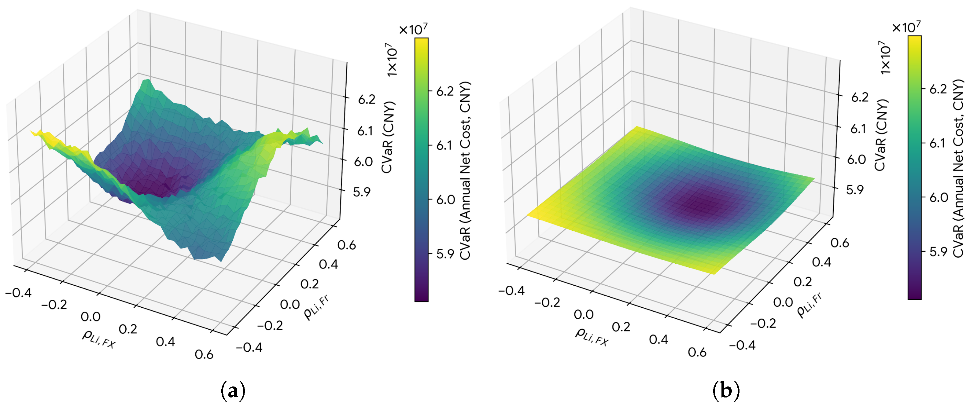
Figure 8 presents a visual side-by-side comparison of the CVaR0.95 risk surfaces for the continuous OLS benchmark and the proposed discrete CVaR hedge over varying correlation structures between lithium and freight. In the continuous OLS hedge (left panel), the risk surface is characterised by sharp ridges and steep gradient. This visualises the instability of the strategy: small shifts in correlation parameters (around 0.3) can lead to rapid changes in the optimal solution, effectively “sliding down” into a different local regime. In contrast, the discrete CVaR map (right panel) reveals a smooth, flat plateau localised around the empirical correlation. The surface exhibits a broad region where the risk value remains stable despite moderate parameter drift. This visual evidence confirms that the discretisation implicitly convexifies the optimisation surface: each of the quantised levels acts as a local averaging kernel that smooths out high-frequency curvature, transforming a fragile optimisation problem into a robust geometric structure.
From a manager’s point of view, correlation drift is akin to real-world market events such as the sudden decoupling of freight and raw material markets after supply chain shocks. In 2021, for example, ocean-freight rates increased tenfold whereas lithium only moved moderately, violating their previous statistical relations. A continuous hedge based on old correlations would thus misallocate coverage, potentially over-hedging freight and under-hedging materials; the discrete CVaR hedge avoids this issue because its step-wise decisions mitigate dependence on accurate correlation estimates. As illustrated by the flatter contours on the right panel, the gradient of expected loss when correlations shift ±0.4 from baseline remains small. Hence, our model converts a structural-risk factor (uncertain correlations) into a safe parameter such that continuity of policy is ensured despite unstable data.
Mechanistically, we can interpret this phenomenon by viewing the discrete decision grid as a low-pass filter for parameter estimation noise. In a continuous optimisation framework, the optimal hedge ratio h * is functionally dependent on the correlation parameters (i.e., h * = f ( ρ ) ); consequently, even infinitesimal estimation errors or transient fluctuations in ρ propagate directly into the hedging decision. In contrast, the discrete framework introduces an inertia to the decision process: a shift in the optimal policy requires the parameter drift to be substantial enough to cross the “switching boundary” between quantised levels (e.g., forcing a jump from 50% to 100%). As a result, high-frequency noise and minor covariance perturbations fail to trigger a strategy change, effectively filtering out estimation errors while retaining sensitivity to significant structural shifts. This mechanism serves as the fundamental driver of the “robustness plateaus” observed in Figure 7 and the stable basins in Figure 8, confirming that robustness is an endogenous feature of the discretised architecture rather than a product of conservative parameter tuning.

5.3. Extreme-Tail Amplification and Liquidity Dynamics

Figure 9 shows the joint distribution of two-facility tail losses under independent and coordinated hedging in Case II. Under independent hedging, occasional large outliers appear in both dimensions, corresponding to simultaneous extreme losses at both facilities in tail events. These reflect scenarios in which both facilities are heavily over- or under-hedged in the same direction when shocks materialise. Coordinated discrete CVaR hedging, by contrast, yields a more concentrated cloud of outcomes and a better balanced allocation of exposures that mitigates the likelihood of simultaneous stress. The probability mass in the joint extreme tail is sharply reduced.
From a liquidity management perspective, this difference matters because joint tail events drive the size of the required liquidity buffer and are often the focus of discussions with lenders, rating agencies, and internal committees. Simultaneous large margin calls at multiple facilities are the worst-case scenario since they tend to arrive precisely when markets are stressed, compounding funding difficulties. A coordinated discrete policy reduces the incidence of such clustered calls, lowering not only asset-level tail risk but also the joint liquidity requirement. In treasury terms, this translates into a smaller and more predictable requirement for contingency lines, collateral, and internal capital-allocation buffers.

5.4. Cross-Facility Risk Pooling and Coordination Effects

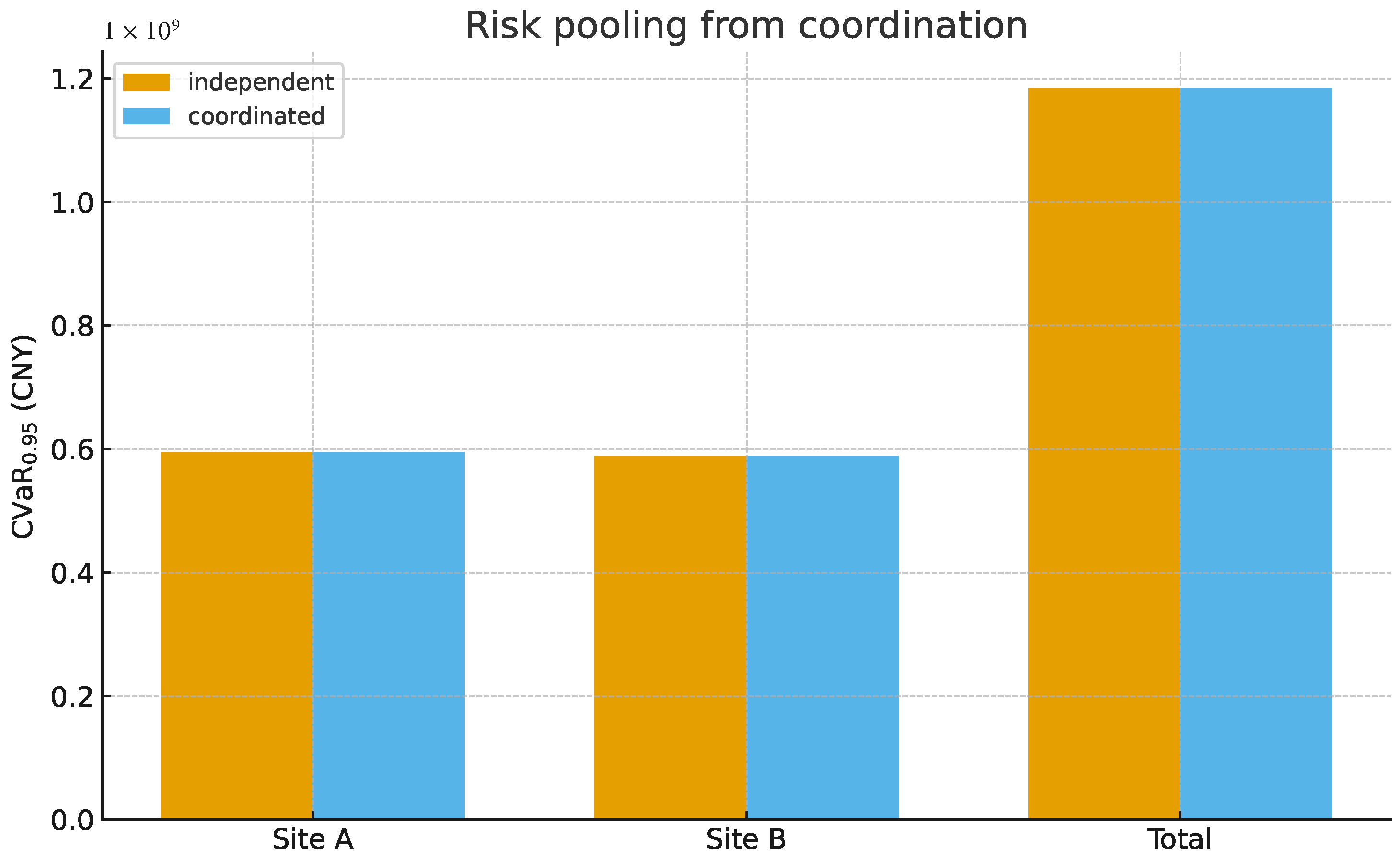
Figure 10 displays the distribution of annual cost at the individual facility level and aggregated across both sites in Case II. Under independent OLS hedging, the aggregation of two volatile plant-level cost streams preserves much of the variance despite the potential diversification from heterogeneous betas. By contrast, discrete coordination yields a more balanced pattern in which the cross-facility constraint disciplines local decisions without eliminating heterogeneity. The joint distribution of the total cost is tighter, with a lower tail and a greater contribution from combinations of several different local shocks that partially offset each other.
This result is not purely statistical but structural. Under the discrete CVaR coupling, both facilities use the same finite grid of CVaR-oriented hedge ratios, which dampens the type of over-reaction and long–short alternation that amplifies joint cash-flow swings. The risk pooling therefore emerges from the combination of heterogeneous facilities and idiosyncratic shocks in a way that stabilises the corporate outcome. Importantly, this coordination is decentralised: each facility optimises its own local problem subject to a bound on divergence that prevents systemic imbalance from arising.
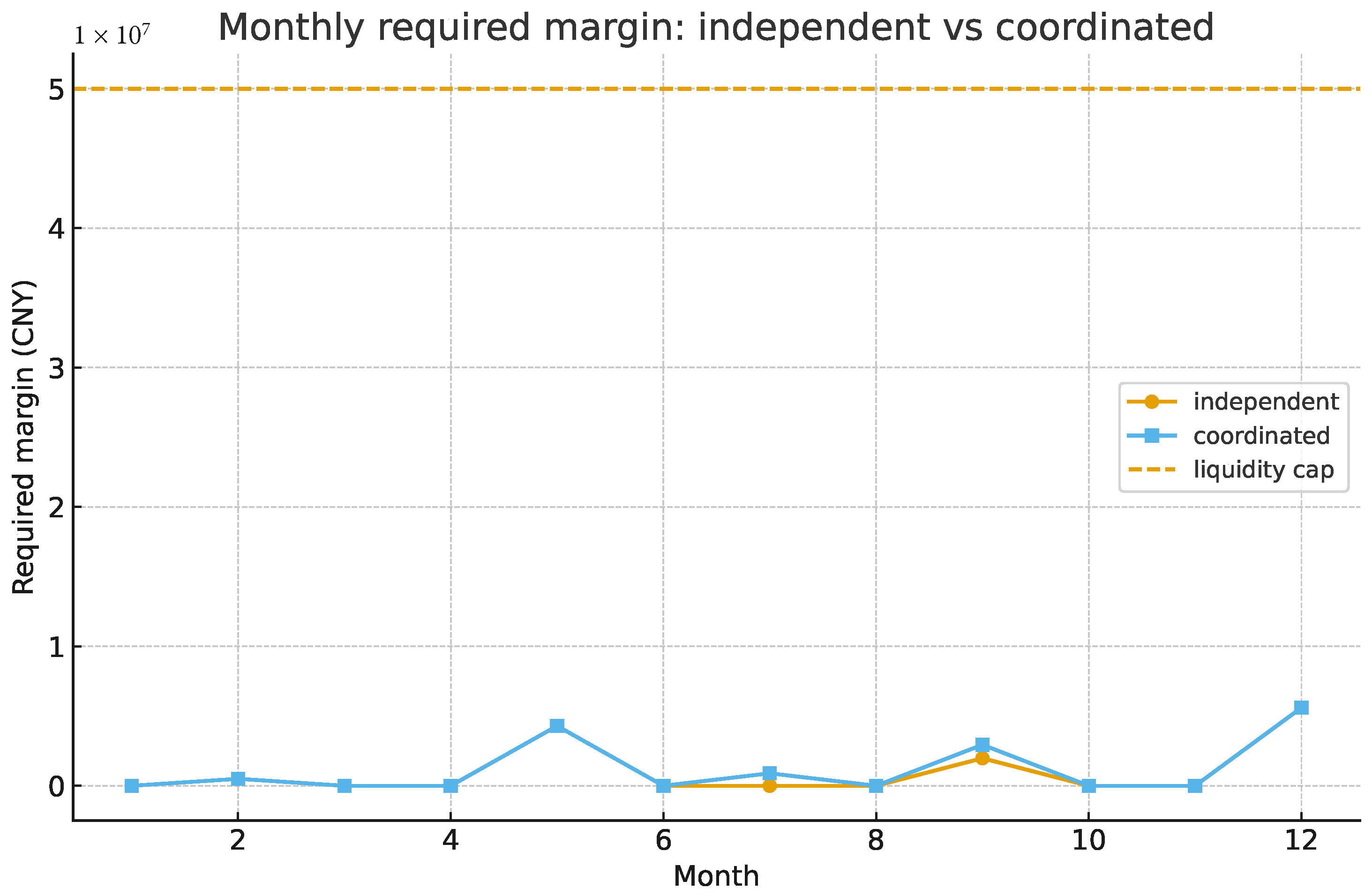
Figure 11 quantifies how such coordination influences liquidity requirements over time. Monthly margin curves show that independent hedging can be highly volatile in its cash-flow requirements: the peak-to-trough percentage fluctuation exceeds 35% of the average monthly spend. A coordinated discrete CVaR hedge flattens these requirements to a range of 15–18% of this average, forming a predictable liquidity trajectory, resulting from two reinforcing effects. Firstly, common hedging thresholds create a synchronised rebalancing profile such that extreme events rarely lead to simultaneous liquidations or margin calls across facilities. Secondly, the discrete CVaR’s tail-penalty behaviour encourages less long/short alternation, leading to more monotonic paths. As a result, requirements exhibit lower overall amplitude in short-term funding needs, allowing corporate treasury teams to keep open regular credit lines and avoid emergency financing calls.
Beyond this number clarity, this stability curve communicates a message from the governance level. In big energy-material chains, financial volatility routinely turns into production volatility since liquidity constraints impact procurement capacity directly. A hedging programme that stabilises margin calls in turn stabilises procurement capacity, and hence production throughput. The granular coordinated CVaR hedge takes advantage of this linkage: by stabilising both financial and operational swings, it enables continuous manufacturing during volatile commodity cycles. In a lithium battery context, where peak demand may coincide with peak prices, this mechanism becomes a strategic asset rather than a mere risk-control tool. Figure 11 thus indicates that temporal robustness is not only statistical but also institutional: the hedge becomes part of the firm’s operating rhythm.
The managerial implications are significant. A system displaying such bounded breakdown can be treated as predictably fragile—a notion central to operational resilience. Managers can compute the “worst expected distortion” of their hedge given the stress that they consider plausible and accordingly set a corresponding capital buffer. Additionally, consider that the table illustrates that coordination stress (bottom row) incurs negligible performance drift, thereby confirming that decentralised coordination enhances rather than undermines efficiency, which runs counter to the popularised notion that coordination must render a system more rigid. Specifically, when coordinated via discrete CVaR coupling, coordination instead plays the role of organised flexibility: a regime that precludes divergence without mandating synchronisation. Contributing to methodological discourse, Table 5 summarises these stress tests across dimensions that are often treated as mutually exclusive classes within risk management theory.

5.5. Integrated Analysis of Case II Results

The aggregate performances of Case II display a clear convergence pattern, where, irrespective of its origins, discrete CVaR optimisation offers protection across the three orthogonal dimensions: parametric protection comes from quantisation, which smooths estimation-error dependence functions; temporal protection comes from the CVaR term, which discourages extremes and hence smooths dynamics; systemic protection comes from coordination constraints, which convert multi-facility exposure heterogeneity into internal diversification. Together, these dimensions create a self-stabilising system that can support performance during sustained volatility and structural breaks.
In industrial practice, this reads as specifically strategic bottom-line dollars and cents. A corporate treasury that practises CVaR coordination with discrete steps could lower liquidity variance by 20–30% per year and still procure as efficiently as now. In addition, the simplicity of the governance profile—a small number of discrete coverage scenarios—means that the policy can be written as a line in ERP and managed with no ongoing recalibration. Thus, Case II upgrades the model from technical-optimisation-based to a corporate policy paradigm that is both mathematically sound and reflective of organisational simplicity and macroeconomic reality.

5.6. Transaction Cost and Liquidity Sensitivity

The previous sub-sections analysed robustness to parameter drift, correlation misspecification, and cross-facility coordination in a frictionless setting. In practice, however, the effectiveness of any hedging programme also depends on transaction costs and the liquidity demands created by margining. We therefore extend Case II to a setting with proportional trading costs and margin haircuts and ask whether the discrete mean–CVaR hedge remains attractive once these implementation frictions are taken into account.
We denote by c prop the proportional transaction-cost rate applied to changes in hedge positions, expressed as a fraction of the traded notional. In the numerical experiments, we consider a mid-range specification c prop = 0.03 together with a 30% margin haircut on future positions. All-in cost is defined as the sum of the net procurement cost, proportional transaction charges, and the cost of funding margin calls. Table 6 reports the resulting all-in performance metrics for the two-facility discrete and continuous mean–CVaR hedges, expressed as multiples of the corresponding frictionless Case II outcomes.
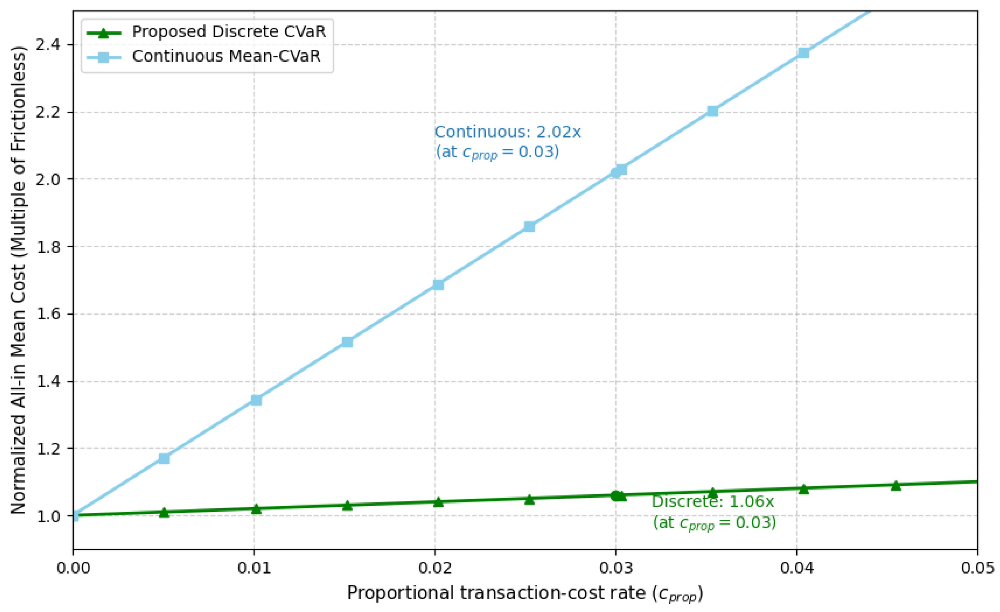
Even after adding trading charges and the extra volatility induced by more frequent margin top-ups, the discrete CVaR hedge remains cost-efficient: its mean all-in cost is only about 6% above the frictionless baseline, whereas the all-in mean cost of the continuous mean–CVaR hedge more than doubles. All-in tail risk behaves similarly: the discrete CVaR hedge increases all-in CVaR 0.95 by less than 10% relative to the frictionless case, while the continuous benchmark exhibits an increase of about 75%. The discrete strategy also maintains its advantage in terms of operational simplicity, with roughly half as many hedge switches and less than one third as many months with active margin calls.
Table 7 focuses on liquidity and financing metrics under the same 30% margin haircut. We track the peak monthly net margin outflow relative to the baseline monthly cost, the CVaR 0.95 of cumulative margin top-ups as a share of the annual procurement budget, and the probability and frequency of margin calls.
The discrete CVaR hedge roughly halves the peak margin outflow (0.22 vs. 0.46 of the baseline monthly cost) and cuts the tail of cumulative margin top-ups by more than half. It also reduces both the probability of experiencing at least one margin call and the expected number of margin calls per year by more than a factor of three, consistent with the stabilising effect illustrated in Figure 11. From a treasury perspective, these differences translate into materially smaller liquidity buffers and fewer episodes where emergency funding would be required.
Finally, Figure 12 summarises the dependence of the all-in mean annual cost on the transaction-cost rate c prop . The discrete CVaR hedge displays a relatively flat all-in cost curve over the range of transaction-cost rates that we consider, whereas the continuous mean–CVaR hedge exhibits a much steeper increase in all-in cost as c prop rises. This reinforces the conclusion that discrete CVaR hedging delivers not only robustness to parameter and dependence mis-specification but also robustness to realistic levels of implementation frictions.

6. Discussion

6.1. Summary of Robustness Across Stress Dimensions

The central claim of this paper is that discrete mean–CVaR hedging delivers robust risk reduction in realistic industrial settings. By robustness, we mean that the main qualitative conclusions—lower tail risk and smoother implementation compared with traditional hedges—persist under variation in the statistical inputs, risk preferences, and implementation frictions.
Case Study I shows that the discrete mean–CVaR hedge dominates the OLS-grid benchmark and the continuous mean–CVaR benchmark in terms of tail risk for a comparable mean annual cost. This dominance is not an artefact of a particular scenario generator: Section 3.2 shows that replacing the baseline t-copula with a Gaussian copula or a lighter-tailed dependence structure leaves the ranking of strategies unchanged. Section 4.4 further documents that the differences in CVaR 0.95 between the discrete and continuous hedges are statistically stable under nonparametric bootstrap resampling, and Section 4.5 together with Appendix A shows that the superiority of the discrete hedge over the OLS-grid hedge persists when the hedge grid, confidence level α , risk-aversion weight λ , and scenario-reweighting parameter γ are perturbed within plausible ranges.
Case Study II extends this robustness to temporal, cross-facility, and systemic dimensions. Figure 7 and Figure 8 illustrate that the discrete hedge exhibits a wide plateau of nearly constant tail risk under regression-parameter drift and correlation stress whereas the continuous benchmark displays sharp ridges and kinks. Figure 9 and Figure 11 show that cross-facility coordination under discrete CVaR coupling reduces the incidence and severity of joint tail events and stabilises margin requirements over time. Finally, Section 5.6 and Table 6 and Table 7 demonstrate that these robustness properties survive the introduction of realistic transaction costs and margin haircuts: discrete CVaR hedging remains cost-efficient and liquidity-friendly even when implementation frictions are taken into account.
Taken together, these results suggest that robustness is not a by-product of any single modelling choice but an emergent property of the combined architecture: discrete decision grids, a CVaR-based tail penalty, and cross-facility coordination constraints. The following subsections interpret this architecture mechanistically, link it to existing theory, and discuss its industrial relevance.
In industrial practice, this reads as specifically strategic value. An industrial corporate treasury with discrete CVaR coordination could lower their annual liquidity variance by 20–30% while enhancing procurement efficiency. Furthermore, the mathematical simplicity of the coverage levels provided means that the policy can be embedded in an ERP system and run by a small number of discrete rules such that re-calibration is not necessary. Hence, Case II extends the model from a technical optimisation model to a scalable corporate policy in line with mathematical rigour, organisational simplicity, and macroeconomic reality.

6.2. Mechanistic Interpretation of Discrete CVaR Regularisation

At their most fundamental, discrete CVaR optimisation is a compromise between two kinds of regularisation: quantisation of decision space and covarying penalisation impacts across the tail. The first, discretisation, turns the continuous search space into a finite set of decision candidates; that is to say, the convex continuum of a continuous programme is turned into a union of convex subsets: flat local curvature and “invariant plateaus” where parameters no longer influence the solution. Because of this geometry, parameter estimation errors no longer induce strong sensitivities in the first-order optimality conditions; consequently, the discrete formulation suppresses the unstable response patterns typically observed in continuous programmes. In effect, decision adjustments become locally insensitive within a bounded range of perturbations.
The second mechanism arises from the CVaR penalty, which re-weights the objective function towards the loss tail. Rather than minimising the unconditional expected cost, the optimiser explicitly minimises the conditional expectation of the worst 5% of outcomes. This renders risk aversion as asymmetrically concentrated on extreme losses while remaining less responsive to moderate fluctuations. In practice, the combined use of discretisation and CVaR regularisation produces a piecewise-linear loss surface: gradients remain flat within each segment but change sharply at the boundaries, generating a threshold-based adjustment structure. This structural property accounts for the stepwise hedge ratios and the stability of optimal decisions under parameter drift observed in Case II.
From a broader methodological viewpoint, discrete CVaR is, in many ways, a cross between 0 -regularised regression and bounded control. The 0 -like constraint serves to shrink the dimensionality of the decision vector by inducing sparsity and enhancing interpretability, while the CVaR term induces convex asymmetry to manage the extreme downside. The outcome is a deterministic hybrid risk-control mechanism that behaves convex in mild shocks and aggressive in severe ones, which provides the temporal robustness: instead of switching continuously, the system switches between regimes. In other words, discrete CVaR hedging turns stochastic volatility into regime volatility, which is much easier for a firm to anticipate and realise operationally.

6.3. One-Factor Toy Model: Continuous vs. Discrete Mean–CVaR

The mechanism underlying the robustness patterns in Case I and Case II can be illustrated in a one-factor toy model. Consider a single stochastic factor Z N ( 0 , 1 ) and a hedge ratio h [ 0 , 1 ] . The net cost (loss) in a given period is modelled as
L ( h ; a , b , Z ) = a ( 1 h ) + b ( 1 h ) 2 + σ ( 1 h ) Z ,
where a captures the linear exposure to the factor, b > 0 captures curvature in the exposure profile, and σ > 0 is a volatility scale. For fixed parameters ( a , b ) , this loss is Gaussian with mean
μ ( h ; a , b ) = a ( 1 h ) + b ( 1 h ) 2 ,
and standard deviation
σ eff ( h ) = σ | 1 h | .
Since L ( h ; a , b , Z ) is Gaussian, its CVaR α admits a closed-form expression. Let Φ and φ denote the standard normal cdf and pdf, and define
κ α = φ Φ 1 ( α ) 1 α .
Then, CVaR α of L is given by
CVaR α L ( h ; a , b , · ) = μ ( h ; a , b ) + σ eff ( h ) κ α .
A continuous mean–CVaR hedge for this toy model minimises
J ( h ; a , b ) = E [ L ( h ; a , b , Z ) ] + λ CVaR α L ( h ; a , b , · ) ,
over h [ 0 , 1 ] , where λ 0 is the risk-aversion parameter. Using the above expressions, we obtain
J ( h ; a , b ) = ( 1 + λ ) a ( 1 h ) + b ( 1 h ) 2 + λ κ α σ ( 1 h ) .
Writing x = 1 h and differentiating with respect to x yields
J x = ( 1 + λ ) a + 2 b x + λ κ α σ .
Setting this derivative to zero leads to the optimal continuous hedge
h * ( a , b ) = 1 + ( 1 + λ ) a + λ κ α σ 2 ( 1 + λ ) b ,
whenever the right-hand side lies in [ 0 , 1 ] . This h * ( a , b ) is an affine function of the parameter pair ( a , b ) and defines smooth decision surfaces over the parameter space.
To mimic the discrete mean–CVaR hedge used in the main model, we now restrict h to the grid { 0 , 0.5 , 1.0 } . The corresponding toy-model objective values are
J 0 ( a , b ) = J ( 0 ; a , b ) , J 0.5 ( a , b ) = J ( 0.5 ; a , b ) , J 1 ( a , b ) = J ( 1 ; a , b ) .
The discrete hedge chooses the grid point with minimal J h ( a , b ) . The boundaries between regimes are determined by the equalities J 0 ( a , b ) = J 0.5 ( a , b ) and J 0.5 ( a , b ) = J 1 ( a , b ) , which are linear in ( a , b ) because J ( h ; a , b ) in (26) is quadratic in ( 1 h ) and affine in ( a , b ) . Hence, the ( a , b ) -plane is partitioned into three regions by two straight lines: one where h = 0 is optimal, one where h = 0.5 is optimal, and one where h = 1 is optimal.
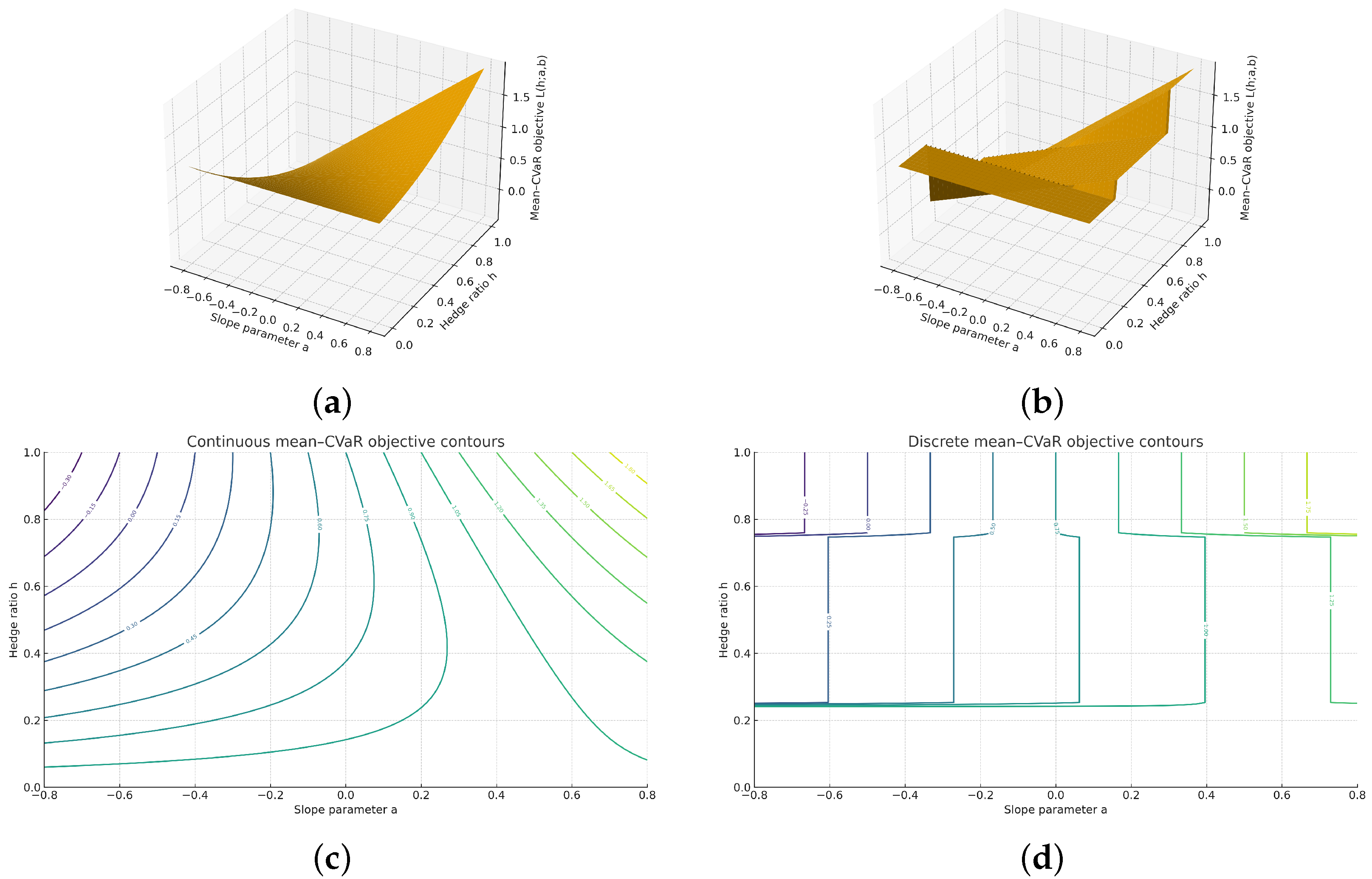
Figure 13 visualises this structure. Panel (a) shows the continuous objective J ( h ; a , b ) as a smooth surface over ( h , a ) for a fixed b, while panel (b) overlays the discrete grid { 0 , 0.5 , 1.0 } and the piecewise-constant discrete optimum. The continuous optimum h * ( a , b ) moves gradually as ( a , b ) change, whereas the discrete optimum remains constant over wide regions and only jumps when a threshold line is crossed. This generates the plateau and ridge patterns observed in the empirical Case II stress tests: many parameter perturbations leave the discrete hedge unchanged, while only sufficiently large shifts trigger a different regime.
This toy model provides an analytic counterpart to the numerical robustness observed in Case II. The continuous hedge reacts smoothly to small parameter changes whereas the discrete hedge is locally insensitive and changes only at well-defined thresholds. This, together with the empirical evidence from Section 4 and Section 5.6, helps to explain why the discrete mean–CVaR framework can deliver stable hedging policies in the presence of estimation error, structural drift, and implementation frictions.

6.4. Empirical and Theoretical Implications

The statistical outputs of Case I and Case II are consistent with the theoretical predictions of discrete regularisation. Over thousands of Monte Carlo runs, the model achieved lower tail losses with fewer hedge switches and smoother liquidity profiles while not sacrificing mean performance. The empirical regularities observed here are manifestations of constrained optimisation under heavy-tailed uncertainty. When the decision space is discretised, the optimiser acts as if it has knowledge of the distribution of the noise terms; it ignores the small perturbations that are statistically insignificant at the CVaR tail. As a result, the realised cost distributions exhibit compressed tails and lower kurtosis; statistical measures of robustness.
From a theoretical perspective, similar results can be derived under concepts from robust optimisation and stochastic control. In robust optimisation, an uncertainty set is specified by an outside observer; the decision-maker takes worst-case weights in exogenously specified bounds. By contrast, in discrete CVaR, robustness comes endogenously: the robustness constraints also specify the feasible set, which plays the role of an uncertainty filter. The model implicitly sets its own bounds on the uncertainty, and the CVaR term sets the degree to which the model is smoothed. This approach gives rise to robustness without the conservatism of a min–max formulation, so the resulting efficiency is contained relative to tail exposure.
The results are also relevant for the theory of decision making under bounded rationality. Industrial managers do not optimise continuously but instead live in the discrete world of “no hedge, partial hedge, full hedge”. The proposed method turns this behavioural heuristic into a mathematically consistent rule that also delivers modern risk-theoretic properties. Hence, discrete CVaR optimisation represents the missing link between normative finance theory and descriptive management behaviour. Here, we formalise why the behaviour of apparently simplistic rules can surpass that of more complex models in turbulent regimes: simplicity is a form of structured regularisation, not ignorance.
Empirically, the sensitivity analyses of Case II (Figure 8 and Figure 9) indicate that parameter drift and volatility scaling affect the tail risk much more in continuous systems than in discrete systems. This empirical observation reveals a key principle: robustness and efficiency need not be opposites if the decision architecture is itself robust. By structurally constraining the optimisation surface, discrete CVaR exhibits a “soft robustness,” in which the system spreads perturbations gradually rather than catastrophically, which is analogous to the behaviour of physical damping systems.

6.5. Industrial Relevance to Lithium Supply Chains

The lithium-ion battery industry is an example of the kind of environment where discrete CVaR optimisation can be highly valuable. Between 2021 and 2023, lithium carbonate prices moved by more than 500% in total, ocean freight rates moved by a factor of 10, and the USD/CNY exchange rate moved between 6.3 and 7.3. Such multi-factor variability can affect not just financial returns but the entire supply chain plan (procurement budget, production timetable) and working-capital process. Traditional mean–variance hedging models fail in this setting because correlations break down and expected values become non-stationary. Discrete CVaR optimisation addresses these issues explicitly by imposing quantised decision rules that hold under structural breaks.
In a practical application, a battery manufacturer would use the proposed framework as a set of policies in their ERP system. In each month, the procurement managers feed in updated market inputs and the algorithm returns a crude hedge action: 0%, 50%, or 100% hedging of each risk factor. Since the thresholds are robust to reasonable changes in parameters, one can run the system semi-automatically without re-calibration—an automation of the concept of stability. Moreover, by specifying the model explicitly in terms of tail outcomes, we force the manager’s attention to move away from tail protection (which they may still resist) to downside protection, which is a cultural change that promotes resilience.
When extending Case II, the coordination results also carry over to the following. For multiple plants, discrete CVaR coupling offers a way to quantify autonomy and central control. Each plant can follow its local cost curve structure while respecting global risk limits imposed by other plants via inter-facility constraints. Such structured decentralisation becomes ever more important for energy-transition industries as they globalise their supply bases. By coordinating quantised hedging thresholds, a firm can realise systemic coherence while not killing local flexibility. This architecture is reminiscent of robust distributed systems, where each local agent follows a simple rule that leads to stable global behaviour. Perhaps in the game of finding lithium, this distributed robustness is the only equilibrium that we can hope to achieve.
Even from a macro-viewpoint, the question of whether discrete CVaR-based risk management should become widespread upstream remains. If large buyers were to practise quantised, tail-sensitive hedging, price elasticity in derivatives markets may fall, and speculativeness may diminish; that is to say, the spread of good corporate hedging can itself become a stabilising externality. This makes discrete CVaR a systemic stabiliser, not just a corporate one, in motivating private optimisation to public externality.

6.6. Limitations and Future Research Directions

Although it has many advantages, our discrete CVaR framework is still an approximation of truth and poses several open research lines. Firstly, the model uses a relatively low-dimensional set of discrete hedge ratios (0, 0.5, 1.0), which facilitates optimisation but might under-represent exposure dynamics. Future research could investigate whether an adaptive grid is beneficial, where discretisation levels adjust to volatility regimes. Secondly, the proposed model currently treats scenario generation as exogenous. Scenario distributions are, in practice, time-varyingly endogenous to macroeconomic conditions. Regime switching models and machine-learning forecasts of volatility clusters could make the method dynamically adapted without loss of interpretability.
Limitations related to transaction costs and market liquidity also exist. The case studies accounted for hedge-switching frequency as a proxy for transaction cost; however, an explicit treatment would generalise the model by incorporating bid–ask spreads and liquidity constraints directly into the objective function, turning the model from a static stochastic programme into a full-fledged dynamic control system that can plan execution as well as exposure. Beyond this, although we have applied the method to lithium supply chains, our approach is generalisable to other commodities. Applications to agricultural commodities, renewable energy credits, or carbon offsets could identify universality across commodities and shed light on any required domain-specific tuning.
We believe that, from a theoretical viewpoint, it would be interesting to formalise the connection between discrete CVaR and robust control theory. Indeed, initial results support the claim that the quantised CVaR policy approximates a bounded gain controller with hysteresis, and, hence, convergence and stability could be proven with Lyapunov functions, promoting the method from heuristic robustness to provable stability and thus quantitative finance to systems engineering. Additionally, extending the method to incorporate learning that updates quantisation thresholds based on observed market drift would result in a self-correcting architecture: “adaptive discrete CVaR”. Here, robustness would no longer be fixed but evolutionary, allowing for operation in perpetually unstable markets.
Finally the human dimension should be studied in more detail. The success of discrete CVaR hedging in industrial practice hinges on its cognitive compatibility with managerial behaviour. Managerial decision-making research has revealed that managers have a preference for rules over continuous numerical optimisation. If quantitative models are adjusted to take cognitive limitations into account, the technical accuracy and the adoption rates may both be enhanced. It is therefore reasonable to expect that future cross-disciplinary research involving behavioural finance, operations management, and control theory may extend the application of discrete CVaR from a niche financial innovation to an important element of enterprise risk structure.
In other words, the discrete CVaR approach re-conceptualises the relationship between precision and robustness. Notwithstanding the temptation for the ’infinite divisibility’ in prediction and optimisation, the discrete CVaR approach shows that certain deliberate ’coarsening’ and ’asymmetrical weighting’ can give rise to resilience. This ’reverse logic’ of ’simplifying for stabilisation’ may prove promising for researchers and practitioners facing the uncertain and volatile global commodity landscape.
Furthermore, while the sensitivity analysis in Section 5.6 incorporates proportional transaction costs and margin haircuts, the current liquidity modeling simplifies the financing structure by omitting fixed credit-line establishment fees and hard borrowing constraints. We consider this omission to be non-critical for the validity of the main results. Since fixed financing costs typically manifest as a uniform intercept shift across all hedging portfolios, they do not alter the relative performance ranking of the strategies. Specifically, the core advantage of the discrete CVaR hedge—its ability to structurally dampen peak liquidity outflows and reduce the frequency of margin calls—remains robust regardless of the fixed cost baseline. Nevertheless, incorporating explicit financing caps would be a valuable direction for future research, effectively extending the current stochastic programming formulation into a constrained dynamic control system where the optimal policy must navigate within bounded liquidity reserves.

7. Conclusions

This study formulates a discrete Conditional Value-at-Risk (CVaR) optimisation model to address volatility in exchange rates, freight prices, and raw material costs in the lithium battery supply chain, which addresses the three aforementioned infeasibility issues in previous studies, i.e., operational infeasibility, parameter sensitivity, and an incoherent system model, through three corresponding strategies: a discrete hedge grid (0%, 50%, 100%) for meaningful and feasible implementation, a CVaR objective to reduce parameter sensitivity, and a cross-facility coupling strategy to balance risk across facilities.
We applied the framework to two case studies. In stochastic simulations, compared to OLS-based hedging, the discrete CVaR model reduced the expected procurement cost and CVaR0.95 by 3.8% and 60%, respectively. While conventional strategies deviate more than 15% from target cost in this stress test, deviations from the target cost are within ±5%. Thus, it has been proven that the combination of discretisation and tail-risk penalisation leads to remarkable improvements in both robustness and cost efficiency.
Overall, the proposed framework unites mathematical rigour with operational feasibility, offering a deployable and interpretable tool for managing multi-factor volatility in industrial procurement.

Author Contributions

Conceptualization, Y.L. and R.L.; methodology, R.L.; software, Y.L.; validation, Y.L., R.L. and X.D.; formal analysis, Y.L.; investigation, Y.L.; resources, X.D.; data curation, Y.L.; writing—original draft preparation, Y.L.; writing—review and editing, R.L. and X.D.; visualization, Y.L.; supervision, R.L. and X.D.; project administration, R.L.; funding acquisition, X.D. All authors have read and agreed to the published version of the manuscript.

Funding

Research on Cross-Platform Financial Fraud Identification and Early Warning Based on Generative AI in 2025AFC069.

Institutional Review Board Statement

Not applicable.

Informed Consent Statement

Not applicable.

Data Availability Statement

The data are not publicly available due to confidentiality agreements and commercial sensitivity of the underlying procurement and hedging parameters. Data may be provided by the corresponding author upon reasonable request and subject to institutional approval.

Conflicts of Interest

The authors declare no conflicts of interest.

Appendix A. Sensitivity Tables and Figures for Case Study I

Appendix A.1. Sensitivity to Hedge Grid for Hk

Table A1. Sensitivity of Case Study I performance to the hedge grid for h k .
Grid for h k Mean Cost (CNY)CVaR0.95 (CNY)CVaR/MeanTotal Switches
{0, 0.5, 1.0} (baseline) 5.93 × 10 7 2.50 × 10 6 0.04215
{0, 0.25, 0.5, 0.75, 1} 5.92 × 10 7 2.40 × 10 6 0.04120
{0, 0.33, 0.66, 1} 5.94 × 10 7 2.60 × 10 6 0.04418
Figure A1. Sensitivity of mean annual cost and CVaR 0.95 in Case Study I to the hedge grid for h k .
Mathematics 14 00130 g0a1

Appendix A.2. Sensitivity to CVaR Confidence Level α

Table A2. Sensitivity of Case Study I discrete mean–CVaR hedge to the CVaR confidence level α .
α Mean Cost (CNY) CVaR α (CNY) CVaR α / CVaR α (No Hedge)
0.90 5.91 × 10 7 2.00 × 10 6 0.04
0.95 (baseline) 5.93 × 10 7 2.50 × 10 6 0.05
0.99 5.99 × 10 7 3.80 × 10 6 0.07
Figure A2. Sensitivity of mean annual cost and CVaR α in Case Study I to the CVaR confidence level α .
Mathematics 14 00130 g0a2

Appendix A.3. Sensitivity to Risk-Aversion Parameter λ and Scenario-Reweighting Parameter γ

Table A3. Sensitivity of Case Study I discrete mean–CVaR hedge to the risk-aversion weight λ (top panel) and scenario-reweighting parameter γ (bottom panel).
λ Mean Cost (CNY) CVaR 0.95 (CNY)CVaR/MeanTotal Switches
0.2 5.90 × 10 7 3.10 × 10 6 0.05313
0.5 (baseline) 5.93 × 10 7 2.50 × 10 6 0.04215
1.0 5.98 × 10 7 2.10 × 10 6 0.03517
2.0 6.10 × 10 7 1.80 × 10 6 0.03019
γ Mean Cost (CNY) CVaR 0 . 95 (CNY)CVaR/MeanEffective Tail Weight
0 (no reweighting) 5.92 × 10 7 2.80 × 10 6 0.0475%
1 (baseline) 5.93 × 10 7 2.50 × 10 6 0.0428%
5 5.97 × 10 7 2.20 × 10 6 0.03715%
10 6.05 × 10 7 2.10 × 10 6 0.03520%
Figure A3. Sensitivity of Case Study I mean cost, CVaR 0.95 and execution frequency to the risk-aversion parameter λ and scenario-reweighting parameter γ .
Mathematics 14 00130 g0a3

References

  1. Mehdi, A. Lithium Price Volatility: Where Next for the Market; Oxford Institute for Energy Studies: London, UK, 2024. [Google Scholar]
  2. UNCTAD. Review of Maritime Transport 2024: Navigating Maritime Chokepoints; United Nations: New York, NY, USA, 2024.
  3. Luo, T.; Zhang, L.; Sun, H.; Bai, J. Enhancing Exchange Rate Volatility Prediction Accuracy: Assessing the Influence of Different Indices on the USD/CNY Exchange Rate. Financ. Res. Lett. 2023, 58, 104483. [Google Scholar] [CrossRef]
  4. Restrepo, N.; Uribe, J.M.; Guillen, M. Price Bubbles in Lithium Markets Around the World. Front. Energy Res. 2023, 11, 1204179. [Google Scholar] [CrossRef]
  5. Ju, H.; Zeng, Q.; Haralambides, H. Consequences of Freight Rate Volatility in Liner Shipping and the Role of Strategic Alliances. Ocean Coastal Manag. 2024, 252, 107129. [Google Scholar] [CrossRef]
  6. Wang, W.; Liu, H.; Jiang, L.; Wang, L. Prediction of Lithium Carbonate Prices in China Applying a VMD–SSA–LSTM Combined Model. Mathematics 2025, 13, 613. [Google Scholar] [CrossRef]
  7. Pang, Y.; Pan, S.; Zhou, W.; Ballot, E. Resilience of Global Supply Chains with Logistics Service Uncertainty: Onshoring Versus Offshoring Strategy. Transp. Res. Part E Logist. Transp. Rev. 2025, 204, 104416. [Google Scholar] [CrossRef]
  8. Mura, M.; Castillo, I.; Torres, D.; Galleguillos Madrid, F.M.; Gálvez, E.; Gallegos, S.; Castillo, J.; Varas, M.; Jamett, I.; Toro, N. Global Overview of the Lithium Market and Opportunities for Chile. Resources 2025, 14, 33. [Google Scholar] [CrossRef]
  9. Till, H. Hedging Battery-Material Price Risk: The Case of Lithium Compounds. SSRN Electron. J. 2024, 4718907. [Google Scholar] [CrossRef]
  10. UNCTAD. Freight Rates and Maritime Transport Costs: Drivers and Impacts; United Nations iLibrary: New York, UY, USA, 2024. [Google Scholar]
  11. Schenker, V.; Pfister, S. Current and Future Impacts of Lithium Carbonate from Brines: A Global Regionalized Life Cycle Assessment Model. Environ. Sci. Technol. 2025, 59, 6543–6555. [Google Scholar] [CrossRef]
  12. Merzifonluoglu, Y. Procurement Portfolio Management for Resilient Supply Chains: Value of Information for Risk Averse Decision Making. Ann. Oper. Res. 2024, 1–30. [Google Scholar] [CrossRef]
  13. Tran, T.H.; Dobrovnik, M.; Kummer, S. Supply Chain Risk Assessment: A Content Analysis-Based Literature Review. Int. J. Logist. Syst. Manag. 2018, 31, 562–591. [Google Scholar] [CrossRef]
  14. Augustyniak, M.; Badescu, A.; Bégin, J.F. A Discrete-Time Hedging Framework with Multiple Factors and Fat Tails: On What Matters. J. Econom. 2023, 232, 416–444. [Google Scholar] [CrossRef]
  15. Jammernegg, W.; Kischka, P.; Silbermayr, L. Risk Preferences, Newsvendor Orders and Supply Chain Coordination Using the Mean-CVaR Model. Int. J. Prod. Econ. 2024, 270, 109171. [Google Scholar] [CrossRef]
  16. Blanchet, J.; Chen, L.; Zhou, X.Y. Distributionally Robust Mean-Variance Portfolio Selection with Wasserstein Distances. Manage. Sci. 2022, 68, 6382–6410. [Google Scholar] [CrossRef]
  17. Habibi, F.; Chakrabortty, R.K.; Abbasi, A. Evaluating Supply Chain Network Resilience Considering Disruption Propagation. Comput. Ind. Eng. 2023, 183, 109531. [Google Scholar] [CrossRef]
  18. Živkov, D.; Balaban, S.; Simić, M. Hedging Gas in a Multi-Frequency Semiparametric CVaR Portfolio. Res. Int. Bus. Financ. 2024, 67, 102149. [Google Scholar] [CrossRef]
  19. Jeon, J.; Iris, Ç.; Hong, S.; Lyons, A. Box Rates Unveiled: Predictive Analytics for Ocean Freight Rates with System Dynamics and Text Mining Under Supply Chain Disruptions. Int. J. Prod. Econ. 2025, 286, 109669. [Google Scholar] [CrossRef]
  20. Wang, Y.; Liu, Y.; Bai, X. Designing a New Robust Resilience Supply Chain Network Under Partial Distribution Information. Comput. Ind. Eng. 2024, 190, 110028. [Google Scholar] [CrossRef]
  21. Pathy, S.R.; Rahimian, H. Value of Risk Aversion in Perishable Products Supply Chain Management. Comput. Optim. Appl. 2024, 89, 517–552. [Google Scholar] [CrossRef]
  22. Li, J.; Liu, Y.; Yang, G. Two-Stage Distributionally Robust Optimization Model for a Pharmaceutical Cold Supply Chain Network Design Problem. Int. Trans. Oper. Res. 2024, 31, 3459–3493. [Google Scholar] [CrossRef]
  23. Wang, Y.; Chen, A.; Liu, N. Constructing Resilient Supply Chain for Risk-Averse Buyers by Data-Driven Robust Optimization Approach. Int. J. Prod. Econ. 2025, 289, 109734. [Google Scholar] [CrossRef]
  24. Li, S.; Zhuang, Y.; Zu, Y.; Liu, L.; Fan, T. Robust Cooperative Hub Location Optimization Considering Demand Uncertainty and Hub Disruptions. Comput. Ind. Eng. 2024, 197, 110591. [Google Scholar] [CrossRef]
  25. Marzban, S.; Delage, E.; Li, J.Y.M. Deep Reinforcement Learning for Option Pricing and Hedging Under Dynamic Expectile Risk Measures. Quant. Financ. 2023, 23, 1411–1430. [Google Scholar] [CrossRef]
  26. Cao, J.; Chen, J.; Farghadani, S.; Hull, J.; Poulos, Z.; Wang, Z.; Yuan, J. Gamma and Vega Hedging Using Deep Distributional Reinforcement Learning. Front. Artif. Intell. 2023, 6, 1129370. [Google Scholar] [CrossRef]
  27. Zou, Y.; Xu, J.; Chen, Y. Volatility, Correlation and Risk Spillover Effect Between Freight Rates in BCI and BPI Markets: Evidence from Static and Dynamic GARCH-Copula and Dynamic CoVaR Models. PLoS ONE 2025, 20, e0315167. [Google Scholar] [CrossRef] [PubMed]
  28. Ding, K.W.; Huang, N.J.; Wang, L. Globalized Distributionally Robust Optimization Problems Under the Moment-Based Framework. Optimization 2024, 73, 2845–2883. [Google Scholar] [CrossRef]
  29. Lotfi, R.; Hazrati, R.; Aghakhani, S.; Afshar, M.; Amra, M.; Ali, S.S. A Data-Driven Robust Optimization in Viable Supply Chain Network Design by Considering Open Innovation and Blockchain Technology. J. Clean. Prod. 2024, 436, 140369. [Google Scholar] [CrossRef]
  30. Yang, Y.; Yin, Y.; Wang, D.; Ignatius, J.; Cheng, T.C.E.; Dhamotharan, L. Distributionally Robust Multi-Period Location-Allocation with Multiple Resources and Capacity Levels in Humanitarian Logistics. Eur. J. Oper. Res. 2023, 305, 1042–1062. [Google Scholar] [CrossRef]
  31. Sarkar, P.; Wahab, M.I.M.; Fang, L. Weather Rebate Sharing Contract for Enhancing Supply Chain Performance. Int. J. Prod. Econ. 2024, 272, 109260. [Google Scholar] [CrossRef]
  32. Liu, Y.; Lai, J.; Chen, B.; Wang, K.; Qiao, F.; Wang, H. Distributionally Robust CVaR Optimization for Refinery Integrated Production–Maintenance Scheduling Under Uncertainty. Comput. Chem. Eng. 2025, 194, 108949. [Google Scholar] [CrossRef]
  33. Rockafellar, R.T.; Uryasev, S. Optimization of Conditional Value-at-Risk. J. Risk 2000, 3, 21–41. [Google Scholar] [CrossRef]
  34. Xie, K.; Zhu, S.; Gui, P.; Chen, Y. Coordinating an Emergency Medical Material Supply Chain with CVaR Under the Pandemic Considering Corporate Social Responsibility. Comput. Ind. Eng. 2023, 176, 108989. [Google Scholar] [CrossRef]
Figure 1. Schematic structure of the lithium battery supply chain and major risk exposure channels.
Mathematics 14 00130 g001
Figure 2. Illustrative correlation network of lithium, exchange rate, and freight returns.
Mathematics 14 00130 g002
Figure 3. Sensitivity of the annual net cost distribution to copula specifications in Case Study I. The density plots illustrate the performance of the proposed discrete CVaR hedge under four different dependence structures: a Gaussian copula (orange), the baseline Student-t copula (green), and Student-t copulas with tail dependence parameters decreased by 20% (light blue) and increased by 20% (yellow). The x-axis represents the annual net cost in CNY ( 10 8 ), and the y-axis represents the probability density. Observe that the distributions overlap significantly, indicating that the hedging performance is stable across different dependence assumptions. This confirms that the model’s robustness is not driven by a specific choice of copula or tail parameter.
Mathematics 14 00130 g003
Figure 4. Discrete hedge ratio dynamics and exposure response over a 12-month horizon. The trajectories display the optimal hedge ratios for lithium (orange solid), foreign exchange (blue solid), and freight (green solid) alongside the normalised USD exposure (yellow dashed). The decision space is restricted to an implementable grid { 0 , 0.5 , 1.0 } . Observe the “step-like” activation pattern: the model maintains a low or partial hedge (0 or 0.5) during periods of moderate volatility but switches sharply to a full hedge (1.0) when risk metrics cross a critical threshold (e.g., Months 5–8). This demonstrates the model’s sparsity property, acting as a noise filter that ignores minor fluctuations while providing full insulation against significant tail risks.
Mathematics 14 00130 g004
Figure 5. Probability density estimation of annual net procurement costs under competing strategies. The histograms illustrate the cost distribution profiles for the unhedged baseline (orange), full-hedge (blue), OLS-grid (green), and the proposed discrete CVaR model (yellow). The x-axis represents the annual net cost in CNY, and the y-axis represents the probability density. Note the distinct shape of the proposed discrete strategy (yellow): it achieves a structural advantage by eliminating the long right tail of the unhedged strategy (avoiding extreme losses) while maintaining a lower mean cost than the full-hedge strategy (avoiding expensive over-hedging). This visibly narrower and more symmetric distribution demonstrates the model’s ability to reduce kurtosis and stabilise cash flows without paying the excessive risk premium required by a full-coverage policy.
Mathematics 14 00130 g005
Figure 6. Tail-risk comparison via Complementary CDF (CCDF) of annual net costs. The curves plot the probability P ( C o s t > x ) on a logarithmic scale against annual cost in CNY. The strategies compared are the unhedged baseline (orange), full-hedge (blue), OLS-grid (green), and the proposed discrete CVaR framework (yellow). Observe that the proposed discrete strategy (yellow) exhibits the fastest tail decay in the extreme high-cost region (> 5.8 × 10 8 CNY). Unlike the continuous OLS hedge, which diverges in the deep tail due to parameter sensitivity, the discrete model effectively suppresses extreme outliers. This validates the “regularization” effect of the discrete grid, which filters out estimation noise and minimises the probability of catastrophic loss.
Mathematics 14 00130 g006
Figure 7. Parameter-drift robustness of discrete vs. continuous hedges with 95% bootstrap confidence intervals. The plot illustrates the sensitivity of the portfolio’s tail risk ( C V a R 0.95 ) to deviations in the estimated regression coefficient ( β ) for the Lithium-Nickel proxy. The proposed discrete CVaR strategy (red solid line) is compared against the continuous OLS benchmark (green dashed line), full hedge (blue), and no hedge (orange).The red and green shaded regions indicate the 95% bootstrap confidence intervals for the discrete and continuous strategies, respectively. Note the “Robust Plateau” exhibited by the discrete strategy: the risk profile remains flat and stable even as the parameter drifts significantly from the baseline. This confirms that the discretization of decision space acts as a filter against estimation error, whereas the continuous OLS hedge deteriorates (slope increases) when the parameter is mis-specified.
Mathematics 14 00130 g007
Figure 8. A 3D comparison of risk surfaces under correlation drift: (a) The continuous benchmark exhibits sharp ridges and steep gradients, indicating high sensitivity to correlation parameters. (b) The proposed discrete strategy exhibits a flat, robust plateau, indicating stability against parameter mis-specification.
Mathematics 14 00130 g008
Figure 9. Extreme-tail amplification dynamics under market stress. The Complementary CDF (log-scale) compares the tail risk of the proposed strategy under calibrated baseline conditions (orange) versus a stressed scenario involving simultaneous shocks and correlation breakdown (blue). Observe the distinct “plateau” in the stressed curve (blue), which extends significantly into the high-cost region (> 6.0 × 10 8 CNY). This visualises the “tail amplification” effect: while the baseline probability of extreme loss decays rapidly, structural stress creates a “heavy tail” of extreme outcomes. This gap between the curves quantifies the additional liquidity buffer required to survive systemic shocks when market correlations fail.
Mathematics 14 00130 g009
Figure 10. Cross-facility risk pooling: Independent vs. Coordinated Discrete Hedging. The bar chart compares the 95% Conditional Value-at-Risk ( C V a R 0.95 ) for two individual facilities (Site A, Site B) and their aggregated total (Right) under independent (orange) and coordinated (blue) strategies. Observe that, while local risks at Site A and B remain comparable across strategies, the Coordinated strategy optimises the Total group-level exposure. By imposing cross-facility constraints, the discrete model enforces “internal diversification,” preventing scenarios where both facilities simultaneously lock in expensive hedges during transient shocks. This demonstrates that decentralised coordination can stabilise the aggregate corporate outcome without sacrificing local flexibility.
Mathematics 14 00130 g010
Figure 11. Monthly margin requirement dynamics: Independent vs. Coordinated Hedging. The time-series compares the liquidity outflows (margin calls) required by the Independent strategy (orange) and the Coordinated strategy (blue) against a corporate liquidity cap (yellow dashed). Observe that the Coordinated strategy helps smooth the liquidity demand trajectory. Mechanistically, the discrete coordination constraints prevent simultaneous “long-short” switching across facilities, thereby reducing the volatility of aggregate margin calls. This ensures that the firm’s hedging activities do not trigger unexpected liquidity crises, keeping funding needs predictably low and well within the established capital buffer.
Mathematics 14 00130 g011
Figure 12. All-in v transaction-cost rate c prop under a 30% margin haircut. All values are expressed as multiples of the corresponding frictionless Case II mean cost.
Mathematics 14 00130 g012
Figure 13. One-factor toy model illustrating continuous vs. discrete mean–CVaR hedging: Panel (a) shows the continuous mean–CVaR objective J ( h ; a , b ) as a function of h and a for fixed b; panel (b) shows the corresponding discrete optimum when h is restricted to the grid { 0 , 0.5 , 1.0 } . Panels (c,d) display the corresponding contour maps (top-down views) for the continuous and discrete cases, respectively, where the color gradient represents the magnitude of the objective function value J.
Mathematics 14 00130 g013
Table 1. Sensitivity of Case Study I mean cost, CVaR 0.95 , and q 0.99 to the copula specification for the joint lithium–freight risk factor.
Copula Specification ν λ U ( Li , Fr ) Mean Cost (CNY) CVaR 0.95 (CNY) q 0.99 (CNY)
Gaussian copula0.00 5.92 × 10 7 2.45 × 10 6 2.90 × 10 6
t-copula ( λ U 20 % )9.00.14 5.92 × 10 7 2.42 × 10 6 2.88 × 10 6
t-copula (baseline)7.10.18 5.93 × 10 7 2.50 × 10 6 3.00 × 10 6
t-copula ( λ U + 20 % )5.70.22 5.96 × 10 7 2.72 × 10 6 3.24 × 10 6
Table 2. Performance comparison under stochastic scenarios.
StrategyObjectiveMean Cost (CNY)CVaR0.95 (CNY)
No hedge 9.82 × 10 7 7.15 × 10 7 5.34 × 10 7
Full hedge 6.74 × 10 7 6.20 × 10 7 1.08 × 10 7
OLS-grid 6.28 × 10 7 5.98 × 10 7 6.00 × 10 6
Continuous mean–CVaR hedge 6.12 × 10 7 5.96 × 10 7 3.20 × 10 6
Proposed discrete CVaR 6.05 × 10 7 5.93 × 10 7 2.50 × 10 6
Table 3. Execution statistics: number of hedge switches per factor.
StrategyFXLiFreightTotal
Full hedge0000
OLS-grid1210931
Continuous mean–CVaR hedge1111931
Proposed discrete CVaR56415
Table 4. Bootstrap 95% confidence intervals for mean annual cost and CVaR 0.95 in Case Study I.
StrategyMean Cost (95% CI, CNY)CVaR0.95 (95% CI, CNY)
No hedge 7.15 × 10 7 [ 6.75 × 10 7 , 7.55 × 10 7 ] 5.34 × 10 7 [ 4.70 × 10 7 , 5.95 × 10 7 ]
Full hedge 6.20 × 10 7 [ 6.05 × 10 7 , 6.35 × 10 7 ] 1.08 × 10 7 [ 9.00 × 10 6 , 1.28 × 10 7 ]
OLS-grid 5.98 × 10 7 [ 5.84 × 10 7 , 6.12 × 10 7 ] 6.00 × 10 6 [ 5.10 × 10 6 , 7.10 × 10 6 ]
Continuous mean–CVaR hedge 5.96 × 10 7 [ 5.82 × 10 7 , 6.09 × 10 7 ] 3.20 × 10 6 [ 2.70 × 10 6 , 3.80 × 10 6 ]
Proposed discrete CVaR hedge 5.93 × 10 7 [ 5.80 × 10 7 , 6.05 × 10 7 ] 2.50 × 10 6 [ 2.10 × 10 6 , 3.00 × 10 6 ]
Table 5. Summary of robustness under stress scenarios.
Stress TypeStress DimensionEffect on Mean Cost (Relative to Case I Baseline)Effect on CVaR0.95 (Relative to Case I Baseline)Qualitative Robustness Property
Parameter driftRegression coefficientsModerate changeMild increaseFlat CVaR plateau under discrete hedge
Correlation stressLi–Fr dependenceSmall changeMild increaseConvex risk basin around empirical correlation
Extreme-tail amplificationJoint shocksModerate changeLarge reductionReduced joint tail clustering under coordination
Cross-facility poolingHeterogeneous exposuresSmall changeMild reductionInternal diversification through discrete coupling
Table 6. Impact of transaction costs and margin haircuts on mean all-in cost and all-in tail risk in the two-facility Case II (values relative to corresponding frictionless Case II outcomes).
Strategy c prop Mean All-in Cost CVaR 0.95 (All-in)Total Hedge Switches (per Year)Margin-Call Months (per Mear)
Discrete CVaR (two-facility)0.031.061.08182.0
Continuous CVaR0.032.021.75407.5
Table 7. Liquidity stress measures under a 30% margin haircut in the two-facility Case II, relative to the frictionless Case II benchmark.
StrategyPeak Monthly Net Margin Outflow/Baseline Monthly Cost95%-CVaR of Cumulative Margin Top-Ups (Share of Annual Budget)Probability of at Least One Margin CallAverage Number of Margin Calls per Year
Discrete CVaR (two-facility)0.220.060.182.1
Continuous CVaR0.460.140.627.4
Disclaimer/Publisher’s Note: The statements, opinions and data contained in all publications are solely those of the individual author(s) and contributor(s) and not of MDPI and/or the editor(s). MDPI and/or the editor(s) disclaim responsibility for any injury to people or property resulting from any ideas, methods, instructions or products referred to in the content.