Dynamic Behavior and Exponential Stability of the Modified Moore–Gibson–Thompson Thermoelastic Model with Frictional Damping

Abstract

This paper investigates a modified one-dimensional Moore–Gibson–Thompson (MGT) thermoelasticity model that significantly extends the classical formulation by incorporating two key structural modifications: frictional damping and a novel cross-coupling structure. The system introduces a viscous frictional damping mechanism proportional to the velocity acting on the mechanical (elastic) field, enhancing dissipation, which is a common feature in models extending Green–Naghdi Type III thermoelasticity. The core novelty, however, lies in introducing an additional coupling structure that explicitly links the thermal relaxation effects with the mechanical dissipation effects. This modification moves beyond the standard MGT coupling and is rooted in an effort to model complex visco-thermal interactions, representing the primary contribution to the literature. The well posedness of this modified system is first established using semigroup theory. Through the construction of a new Lyapunov functional, sufficient conditions are then rigorously derived, ensuring the exponential stability of solutions under specific parameter regimes. Furthermore, a critical balance condition is identified between the thermal conductivity and the thermal relaxation time, beyond which the system’s energy decay ceases to be exponential. Finally, numerical experiments employing an explicit–implicit finite difference scheme validate the theoretical findings and illustrate the substantial influence of both the modified coupling and the frictional damping on the system’s long-term energy behavior.

1. Introduction

This manuscript concerns the investigation of one-dimensional Moore–Gibson–Thompson (MGT) model in thermoelasticity with frictional damping:

$$\left\{\begin{array}{c}\rho u_{tt}=\mu u_{xx}-\beta \left({\theta }_{tx}+\tau {\theta }_{ttx}\right)-u_t,\mathrm{in}\left(0,l\right)\times \left(0,\infty \right),\hfill \\ c{\theta }_{tt}+c\tau {\theta }_{ttt}=-\beta u_{tx}+{\left(\kappa {\theta }_t+{\kappa }^{*}\theta \right)}_{xx},\mathrm{in}\left(0,l\right)\times \left(0,\infty \right),\hfill \end{array}\right.$$

(1)

it is subject to the following initial and boundary conditions:

$$\left\{\begin{array}{c}u\left(x,0\right)=u_0\left(x\right),u_t\left(x,0\right)=u_1\left(x\right),x\in \left(0,l\right),\hfill \\ \theta \left(x,0\right)={\theta }_0\left(x\right),{\theta }_t\left(x,0\right)={\theta }_1\left(x\right),{\theta }_{tt}\left(x,0\right)={\theta }_2\left(x\right),x\in \left(0,l\right),\hfill \\ u\left(0,t\right)=u\left(l,t\right)={\theta }_x\left(0,t\right)={\theta }_x\left(l,t\right)=0,t>0,\hfill \end{array}\right.$$

(2)

where u and $\theta$ represent, respectively, the displacement of the solid elastic material and the temperature difference. The coefficients of the system are positive and can be described as follows (

Table 1. Physical meaning of the coefficients.

Coefficients	Meaning
$\rho$	The mass density.
$\mu$	Shear modulus of elasticity.
$\beta$	Thermoelastic coupling
c	Specific heat at constant strain (the heat capacity of the system).
$\tau$	Relaxation time parameter, accounting for memory effects in the medium.
$\kappa$	Thermal conductivity (non-Fourier).
${\kappa }^{*}$	Heat conduction strength.

).

The partial derivatives presented in system (1) can be interpreted physically as follows (

Table 2. Physical meaning of the partial derivatives.

Partial Derivatives	Meaning
$u_t$	Particle velocity
$u_{tt}$	Acceleration
$u_{xx}$	Spatial curvature–strain gradient
$u_{tx}$	Rate of strain generates heat via deformation
${\theta }_t$	Local rate of temperature change
${\theta }_{tt}$	Temperature acceleration
${\theta }_{ttt}$	Jerk in thermal response (higher-order memory)
${\theta }_{tx}$	Heat rate per unit length variation
${\theta }_{ttx}$	Delayed/relaxed thermoelastic force
${\theta }_{xx}$	Heat diffusion (classical Fourier)
${\left(.\right)}_{xx}$	Heat flow divergence

).

The physical meaning of each term in the above system can be summarized in the following

Table 3. Physical meaning of each term in the system.

Term	Meaning
$\rho u_{tt}$	Inertial force: Mass × acceleration
$\mu u_{xx}$	Elastic restoring force: From Hooke’s law (stress from strain)
$-\beta {\theta }_{tx}$	Thermal expansion force: Thermoelastic stress from time-varying temperature gradient
$-\beta \tau {\theta }_{ttx}$	Thermal memory corrections: Delayed thermal force
$-u_t$	Linear friction/damping: Models energy loss via viscosity or structural resistance
$c{\theta }_{tt}$	Thermal inertia: Resistance to rapid temperature acceleration
$c\tau {\theta }_{ttt}$	Thermal memory: Delayed thermal force
$-\beta u_{tx}$	Mechanical-to-thermal conversion: Work done by stress contributes to heat
${\left(\kappa {\theta }_t+{\kappa }^{*}\theta \right)}_{xx}$	Generalized heat flux divergence: Includes conduction and temperature relaxation

.

The present study distinguishes itself from previous works by employing the Moore–Gibson–Thompson (MGT) model of type III in thermoelasticity, which incorporates the Green–Naghdi type III heat conduction law. Unlike classical Fourier or type III models, this formulation accounts for finite-speed thermal wave propagation and allows for a more accurate description of dynamic thermal responses in microstructured or highly sensitive materials. Furthermore, the introduced additional coupling structure establishes a novel interaction between the thermal and mechanical fields, enhancing the predictive capacity of the model and enabling the rigorous analysis of exponential stability under specific boundary and initial conditions. This work also advances the mathematical understanding of the asymptotic behavior of solutions, deriving new stability results and necessary conditions, thereby providing insights that are not addressed in previous studies. Consequently, the modified MGT system offers both theoretical and practical advancements, expanding the range of applications in modern thermoelasticity, including smart materials and high-frequency thermal phenomena.

The physical meaning of the boundary conditions on the displacement can be explained as clamped ends, which means that the body is fixed at both ends (no displacement) and for the Neumann conditions on the temperature means that there are no heat flux across boundaries (thermally insulated body). For the problem to be well posed and to ensure the existence and uniqueness of the solution, the initial data must satisfy certain regularity requirements. Specifically, the initial functions for displacement and temperature difference, $u_0\left(x\right)$, $u_1\left(x\right)$, ${\theta }_0\left(x\right)$, ${\theta }_1\left(x\right)$, and ${\theta }_2\left(x\right)$, are assumed to belong to carefully selected functional spaces (e.g., specific Sobolev spaces or their products) that are consistent with the energy space of the system. This selection guarantees the necessary regularity and compatibility for the solution across the spatial domain and over the time interval.

A crucial hypothesis regarding the model’s coefficients is imposed to ensure the mathematical validity and physical stability of the system. Specifically, assume that

$$\kappa >{\kappa }^{*}\tau ,$$

(3)

which is indispensable for the well-posedness and stability analysis of the MGT thermoelastic system. The product ${\kappa }^{*}\tau$ captures the interaction between the thermal conductivity $\left({\kappa }^{*}\right)$ and the thermal relaxation time $\tau$. Although $\tau$ is not a classical time delay, it represents a relaxation time associated with the physical behavior of the material or fluid, ensuring causality and finite propagation speed. This product therefore quantifies the level of memory or non-instantaneous response of the medium to thermal disturbances. The quantity ${\kappa }^{*}\tau$ plays a critical role in several stability results (including exponential stability in MGT-type systems). Its interpretation is straightforward: when $\tau$ is large (indicating a strong memory effect), the system requires higher thermal conductivity $\kappa$ to remain stable. Conversely, if ${\kappa }^{*}\tau$ is too small, the system is unable to dissipate thermal energy sufficiently fast, which may lead to sustained oscillations or instability.

Some researchers have argued that type III heat conduction violates the principle of causality, which motivated the development of Choudhuri’s theory [1] and also led to the introduction of the Moore–Gibson–Thompson (MGT) theory. The MGT framework was originally derived from a third-order differential equation formulated within the context of fluid-mechanical considerations that was later reinterpreted as a heat-conduction model, as it incorporates a relaxation parameter within the structure of type III heat conduction. Since its emergence, the MGT theory has attracted significant attention, and the number of studies devoted to it has grown substantially. The model is widely used to describe wave propagation in viscoelastic or thermoelastic media where both memory effects and higher-order dissipation play an essential role.

The Moore–Gibson–Thompson (MGT) thermoelasticity model provides an advanced mathematical and physical framework describing the interaction between mechanical and thermal waves in thermoelastic media. It extends classical and generalized heat-conduction theories, including Fourier’s law (instantaneous heat propagation) [2], the Cattaneo–Vernotte model (finite thermal-wave speed) [3], the Lord–Shulman theory (single relaxation time) [4], and the Green–Lindsay formulation (two relaxation times) [5]. By incorporating higher-order time derivatives and accounting for memory effects, the MGT model captures the coupled thermo-mechanical dynamics with greater accuracy, particularly in regimes where both thermal and elastic wave propagation play a significant role. The introduction of a third-order time derivative in the heat-conduction equation enables the MGT formulation to overcome key limitations of earlier models, providing a more realistic description of materials and processes in which classical and generalized theories fall short.

Many investigations have addressed the asymptotic behavior of solutions to the Moore–Gibson–Thompson (MGT) thermoelasticity model. In [6], it was shown that thermal dissipation alone ensures the exponential stability of the solutions to system (1) and (2) in the absence of frictional damping under condition (3). In [1], the author introduced the Moore–Gibson–Thompson heat conduction equation with two temperatures and established the exponential decay of solutions under suitable constitutive assumptions; in the same study, it was further demonstrated that exponential stability cannot be achieved even in the one-dimensional case for the Moore–Gibson–Thompson thermoelasticity model with two temperatures. Moreover, in [7], the authors examined the MGT thermoelasticity framework for dipolar bodies without the assumption of positive definiteness of the elasticity tensors and proved the instability of the resulting solutions. In [8], the Moore–Gibson–Thompson model for linear thermoelastic deformations of dielectrics was analyzed, and the exponential decay of solutions was established for the rigid solid case. There is a growing body of recent work on the Moore–Gibson–Thompson (MGT) law that addresses existence, uniqueness, well-posedness, decay, and stability properties of solutions in various settings, including equations with memory, damping, and fractional or nonlinear terms. For further details and citations to these studies, the reader is referred to the follwing References [9,10,11,12,13,14,15,16,17,18,19].

The principal objective of this paper is to investigate the mathematical system defined by problems (1) and (2). Initially, we establish the well posedness of the system within the framework of semigroup theory. To gain deeper insight into the existence and uniqueness of solutions to linear evolution equations, we direct the readers to references [20,21,22], which address different classes of these problems. Subsequently, utilizing the energy method, we demonstrate that the considered system exhibits exponential stability, the attainment of which is contingent upon condition (3). Furthermore, we examine the same system (1) and (2) under the assumption of the following parametric relationships:

$$\kappa ={\kappa }^{*}\tau ,$$

(4)

and

$${\chi }^{\prime }=4{\kappa }^{*}{\tau }^2-c>0.$$

(5)

Under condition (4), a singular dissipation mechanism—specifically, the frictional damping incorporated into the elasticity equation subject to condition (5)—enables the construction of an appropriate Lyapunov functional. The application of the multipliers technique (which constitutes the core idea in Lemma 10) guarantees the exponential decay of the solution to system (1) and (2). This condition carries profound physical significance, indicating a precise balance between the material’s capability for heat conduction and its propensity to delay thermal effects. This balance places the system at the edge of stability, where thermal waves are neither fully damped nor allowed to grow unbounded. Finally, the problem is discretized using the finite difference method. We introduce a fixed-point algorithm to solve the discretized problem numerically. The results derived from the numerical experiment, which was implemented using MATLAB software (R2009b), are presented to validate the analytical findings. We also performed a parameter study on a mesh grid to thoroughly analyze the system’s behavior across different computational settings.

Since the boundary conditions on $\theta$ are of Newmann type, we introduce a transformation that allows the use of Poincaré’s inequality on $\theta$. From the second equation in (1) and the boundary conditions, it follows that

$$c{\displaystyle \frac{d^2}{d{t}^2}}{\int }_0^l\theta \left(x,t\right)dx+c\tau {\displaystyle \frac{d^3}{d{t}^3}}{\int }_0^l\theta \left(x,t\right)dx=0.$$

(6)

So, by solving (6) and using the initial data of $\theta$, we obtain

$$\begin{array}{ccc}\hfill {\int }_0^l\theta \left(x,t\right)dx& =& {\int }_0^l{\theta }_0\left(x\right)dx+t\left({\int }_0^l{\theta }_1\left(x\right)dx+\tau {\int }_0^l{\theta }_2\left(x\right)dx\right)\hfill \\ & & -{\tau }^2{\int }_0^l{\theta }_2\left(x\right)dx+{\tau }^2{e}^{-{\displaystyle \frac{t}{\tau }}}{\int }_0^l{\theta }_2\left(x\right)dx.\hfill \end{array}$$

(7)

Consequently, if we let

$$\begin{array}{ccc}\hfill \overline{\theta }\left(x,t\right)& =& \theta \left(x,t\right)-{\displaystyle \frac{1}{l}}\left[{\int }_0^l{\theta }_0\left(x\right)dx+t\left({\int }_0^l{\theta }_1\left(x\right)dx+\tau {\int }_0^l{\theta }_2\left(x\right)dx\right)\right.\hfill \\ & & \left.-{\tau }^2{\int }_0^l{\theta }_2\left(x\right)dx+{\tau }^2{e}^{-{\displaystyle \frac{t}{\tau }}}{\int }_0^l{\theta }_2\left(x\right)dx\right],\hfill \end{array}$$

we get

$${\int }_0^l\overline{\theta }\left(x,t\right)dx=0,\forall t\ge 0,$$

which allows the use of Poincaré’s inequality on $\overline{\theta }$. So, $(u,\overline{\theta })$ satisfies (1) and (2). Therefore, we work with $(u,\overline{\theta })$, but we write $(u,\theta )$ for simplicity.

Outline of the paper. The work is divided as follows. In Section 2, we use the semigroup method to prove the well posedness of problems (1) and (2). In Section 3 and Section 4, we state and demonstrate some technical lemmas needed in the proof of our main result. Section 5 is devoted to the numerical simulation. Finally, the study ends with a conclusion that summarizes the main findings and outlines future directions.

2. The Well Posedness of the Problem

In this section, we give the existence and uniqueness results for the system (1) and (2) using the semigroup theory [23,24]. So, we denote $U={\left(u,v,\theta ,\varphi ,\psi \right)}^T$, where $v=u_t,$ $\varphi ={\theta }_t$ and $\psi ={\theta }_{tt}$. Then, system (1) and (2) can be rewritten as follows:

$$\left\{\begin{array}{c}{\displaystyle \frac{dU}{dt}}-\mathcal{A}U=0,t>0,\hfill \\ U\left(x,0\right)=U_0\left(x\right)={(u_0,u_1,{\theta }_0,{\theta }_1,{\theta }_2)}^T,\hfill \end{array}\right.$$

(8)

where the operator $\mathcal{A}:D\left(\mathcal{A}\right)\subset \mathcal{H}\to \mathcal{H}$ is defined by

$$\mathcal{A}U=\left(\begin{array}{c}v\\ {\displaystyle \frac{1}{\rho }}\left(\mu u_{xx}-\beta {\varphi }_x-\beta \tau {\psi }_x-v\right)\\ \varphi \\ \psi \\ {\displaystyle \frac{1}{c\tau }}\left(-c\psi -\beta v_x+{\kappa }^{*}{\theta }_{xx}+\kappa {\varphi }_{xx}\right)\end{array}\right),$$

with

$$\mathcal{A}=\left(\begin{array}{ccccc}0& I& 0& 0& 0\\ {\displaystyle \frac{\mu }{\rho }}{\partial }_{xx}\left(.\right)& -{\displaystyle \frac{1}{\rho }}I& 0& -{\displaystyle \frac{\beta }{\rho }}{\partial }_x\left(.\right)& -{\displaystyle \frac{\beta \tau }{\rho }}{\partial }_x\left(.\right)\\ 0& 0& 0& I& 0\\ 0& 0& 0& 0& I\\ 0& {\displaystyle \frac{-\beta }{c\tau }}{\partial }_x\left(.\right)& {\displaystyle \frac{{\kappa }^{*}}{c\tau }}{\partial }_{xx}\left(.\right)& {\displaystyle \frac{\kappa }{c\tau }}{\partial }_{xx}\left(.\right)& {\displaystyle \frac{-1}{\tau }}I\end{array}\right).$$

We consider the energy space

$$\mathcal{H}=H_0^1\left(0,l\right)\times L^2\left(0,l\right)\times H_{*}^1\left(0,l\right)\times H_{*}^1\left(0,l\right)\times L_{*}^2\left(0,l\right),$$

where

$$\begin{array}{ccc}\hfill L_{*}^2\left(0,l\right)& =& \left\{u\in L^2\left(0,l\right):{\int }_0^{l}udx=0\right\},\hfill \\ \hfill H_{*}^1\left(0,l\right)& =& \left\{u\in H^1\left(0,l\right):{\int }_0^{l}udx=0\right\}=H^1\left(0,l\right)\cap L_{*}^2\left(0,l\right).\hfill \end{array}$$

$\mathcal{H}$ is a Hilbert space with respect to the following inner product:

$$\begin{array}{cc}\hfill {〈U,\tilde{U}〉}_{\mathcal{H}}& =\rho 〈v,\tilde{v}〉+\mu 〈u_x,{\tilde{u}}_x〉+c〈\varphi +\tau \psi ,\tilde{\varphi }+\tau \tilde{\psi }〉+{\kappa }^{*}〈{\theta }_x,{\tilde{\theta }}_x〉\hfill \\ \hfill & +{\kappa }^{*}\tau 〈{\tilde{\theta }}_x,{\varphi }_x〉+{\kappa }^{*}\tau 〈{\tilde{\varphi }}_x,{\theta }_x〉+\kappa \tau 〈{\tilde{\varphi }}_x,{\varphi }_x〉.\hfill \end{array}$$

(9)

where $〈.,.〉$ is the inner product of $L^2\left(0,l\right)$, and ${∥.∥}_2$ is the associated norm.

Remark 1.

Under the hypothesis $\kappa >{\kappa }^{*}\tau ,$ it is easy to see that (9) defines an inner product. In fact, from (9), we have

$$\begin{array}{cc}\hfill {∥U∥}_{\mathcal{H}}^2& ={〈U,U〉}_{\mathcal{H}}=\rho {∥v∥}_2^2+\mu {∥u_x∥}_2^2+c{∥\varphi +\tau \psi ∥}_2^2\hfill \\ \hfill & +{\kappa }^{*}{∥\tau {\varphi }_x+{\theta }_x∥}_2^2+\tau \left(\kappa -{\kappa }^{*}\tau \right){∥{\varphi }_x∥}_2^2.\hfill \end{array}$$

Hence, since $\kappa >{\kappa }^{*}\tau$, we conclude that ${〈U,\tilde{U}〉}_{\mathcal{H}}$ defines an inner product on $\mathcal{H}$, and the associated norm ${∥.∥}_{\mathcal{H}}$ is equivalent to the usual one.

The domain of $\mathcal{A}$ is given by

$$\begin{array}{cc}\hfill D\left(\mathcal{A}\right)& =\left\{U\in \mathcal{H}\mid u\in H^2\left(0,l\right)\cap H_0^1\left(0,l\right);\theta ,\varphi \in H_{*}^2\left(0,l\right)\cap H_{*}^1\left(0,l\right);\right.\hfill \\ \hfill & \left.v\in H_0^1\left(0,l\right);\psi \in H_{*}^1\left(0,l\right)\right\},\hfill \end{array}$$

where

$$H_{*}^2\left(0,L\right)=\left\{u\in H^2\left(0,L\right),u_x\left(0\right)=u_x\left(L\right)=0\right\}.$$

Clearly, $D\left(\mathcal{A}\right)$ is dense in $\mathcal{H}$. Now, we can give the following well-posedness result.

Theorem 1.

Let $U_0\in \mathcal{H}$, and assume that (3) holds. Then, there exists a unique solution $U\in C\left({\mathbb{R}}_{+},\mathcal{H}\right)$ of problem (8). Moreover, if $U_0\in D\left(\mathcal{A}\right)$, then

$$U\in C\left({\mathbb{R}}_{+},D\left(\mathcal{A}\right)\right)\cap C^1\left({\mathbb{R}}_{+},\mathcal{H}\right).$$

Proof. 

For any $U\in D\left(\mathcal{A}\right)$ and using the inner product, we have

$${〈\mathcal{A}U,U〉}_{\mathcal{H}}=〈\left(\begin{array}{c}v\\ {\displaystyle \frac{1}{\rho }}\left(\mu u_{xx}-\beta {\varphi }_x-\beta \tau {\psi }_x-v\right)\\ \varphi \\ \psi \\ {\displaystyle \frac{1}{c\tau }}\left(-c\psi -\beta v_x+{\kappa }^{*}{\theta }_{xx}+\kappa {\varphi }_{xx}\right)\end{array}\right),\left(\begin{array}{c}u\\ v\\ \theta \\ \varphi \\ \psi \end{array}\right)〉.$$

Then, we obtain

$${〈\mathcal{A}U,U〉}_{\mathcal{H}}=-\left(\kappa -{\kappa }^{*}\tau \right){∥{\varphi }_x∥}_2^2-{∥v∥}_2^2\le 0.$$

(10)

Since the condition $\kappa >{\kappa }^{*}\tau$ holds, then $\mathcal{A}$ is dissipative.

Next, we prove that the operator $\mathcal{I}-\mathcal{A}$ is surjective. For any $F={\left(f_1,f_2,f_3,f_4,f_5\right)}^T\in \mathcal{H}$, we prove that there exists a unique $U\in D\left(\mathcal{A}\right)$ such that

$$\left(\mathcal{I}-\mathcal{A}\right)U=F.$$

(11)

The problem (11) leads to solve the following system:

$$\left\{\begin{array}{c}u-v=f_1\in H_0^1\left(0,l\right),\hfill \\ {\rho }_{1}v-\mu u_{xx}+\beta {\varphi }_x+\beta \tau {\psi }_x=\rho f_2\in L^2\left(0,l\right),\hfill \\ \theta -\varphi =f_3\in H_{*}^1\left(0,l\right),\hfill \\ \varphi -\psi =f_4\in H_{*}^1\left(0,l\right),\hfill \\ {\tau }_1\psi +\beta v_x-{\kappa }^{*}{\theta }_{xx}-\kappa {\varphi }_{xx}=c\tau f_5\in L_{*}^2\left(0,l\right),\hfill \end{array}\right.$$

(12)

with

$$\left\{\begin{array}{c}{\rho }_1=\rho +1,\hfill \\ {\tau }_1=c\left(\tau +1\right).\hfill \end{array}\right.$$

Inserting $v=u-f_1,$ and using (12)₃ and (12)₄, we get

$$\left\{\begin{array}{c}{\rho }_{1}u-\mu u_{xx}+\beta \left(\tau +1\right){\theta }_x={\upsilon }_1\in L^2\left(0,l\right),\hfill \\ {\tau }_1\theta +\beta u_x-\left({\kappa }^{*}+\kappa \right){\theta }_{xx}={\upsilon }_2\in L_{*}^2\left(0,l\right),\hfill \end{array}\right.$$

(13)

with

$$\left\{\begin{array}{c}{\upsilon }_1=\beta \tau {\left(f_3+f_4\right)}_x+\beta f_{3x}+{\rho }_1{f}_1+\rho f_2,\hfill \\ {\upsilon }_2={\kappa f}_{3xx}+\beta f_{1x}+{\tau }_1\left(f_3+f_4\right)+c\tau f_5.\hfill \end{array}\right.$$

To solve (13), we consider

$$B\left(\left(u,\theta \right);\left(\tilde{u},\tilde{\theta }\right)\right)=\mathcal{G}\left(\tilde{u},\tilde{\theta }\right),$$

(14)

where $B:{\left[H_0^1\left(0,l\right)\times H_{*}^1\left(0,l\right)\right]}^2\to \mathbb{R}$ is the bilinear form defined by

$$\begin{array}{cc}\hfill B\left(\left(u,\theta \right);\left(\tilde{u},\tilde{\theta }\right)\right)& ={\rho }_1〈u,\tilde{u}〉+\mu 〈u_x{,\tilde{u}}_x〉+\beta \left(\tau +1\right)〈{\theta }_x,\tilde{u}〉\hfill \\ \hfill & +{\tau }_1\left(\tau +1\right)〈\theta ,\tilde{\theta }〉+\beta \left(\tau +1\right)〈u_x,\tilde{\theta }〉\hfill \\ \hfill & +\left({\kappa }^{*}+\kappa \right)\left(\tau +1\right)〈{{\theta }_x,\tilde{\theta }}_x〉\hfill \end{array}$$

and $\mathcal{G}:H_0^1\left(0,l\right)\times H_{*}^1\left(0,l\right)\to \mathbb{R}$ is the linear form given by

$$\mathcal{G}\left(\tilde{u},\tilde{\theta }\right)=〈{\upsilon }_1,\tilde{u}〉+\left(\tau +1\right)〈{\upsilon }_2,\tilde{\theta }〉.$$

Let $\mathcal{V}=H_0^1\left(0,l\right)\times H_{*}^1\left(0,l\right)$ be equipped with the norm

$${∥\left(u,\theta \right)∥}_V^2={∥u∥}_2^2+{∥u_x∥}_2^2+{∥\theta ∥}_2^2+{∥{\theta }_x∥}_2^2,$$

and using integration by parts, we can easily prove that

$$\begin{array}{cc}\hfill \left|B\left(\left(u,\theta \right);\left(u,\theta \right)\right)\right|& ={\rho }_1{∥u∥}_2^2+\mu {∥u_x∥}_2^2+{\tau }_1\left(\tau +1\right){∥\theta ∥}_2^2\hfill \\ \hfill & +\left({\kappa }^{*}+\kappa \right)\left(\tau +1\right){∥{\theta }_x∥}_2^2\hfill \\ \hfill & \ge M_0{∥\left(u,\theta \right)∥}_{\mathcal{V}}^2,\hfill \end{array}$$

where $M_0=min\left\{{\rho }_1,\mu ,{\tau }_1\left(\tau +1\right),\left({\kappa }^{*}+\kappa \right)\left(\tau +1\right)\right\}.$

Thus, B is coercive. Moreover, we can easily see that B and $\mathcal{G}$ are bounded. Consequently, by the Lax–Milgram Lemma, system (13) has a unique solution $\left(u,\theta \right)\in \mathcal{V}$ satisfying (14).

Substituting u and $\theta$ in (12)₁ and (12)₃, we obtain

$$v\in L^2\left(0,l\right),\varphi \in H_{*}^1\left(0,l\right),$$

and inserting $\varphi$ in (12)₄, we have

$$\psi \in L_{*}^2\left(0,l\right).$$

The application of the regularity theory for the linear elliptic equations guarantees the existence of unique $U\in D\left(\mathcal{A}\right)$ such that (11) is satisfied. Consequently, we conclude that $\mathcal{A}$ is a maximal dissipative operator. Hence, by the Lumer–Phillips theorem (see [21,24]), the well-posedness result of the problem is achieved. □

3. Technical Lemmas

In this section, we state and prove our stability result for the energy of the solution of system (1) and (2) using the multiplier technique. To achieve our goal, we need the following lemmas.

Lemma 1.

Let $U=\left(u,\theta \right)$ be the solution of (1) and (2). Then the energy functional, defined by

$$\begin{array}{ccc}\hfill E\left(t\right)& =& {\displaystyle \frac{1}{2}}\left(\rho {∥u_t∥}_2^2+\mu {∥u_x∥}_2^2+c{∥{\left(\theta +\tau {\theta }_t\right)}_t∥}_2^2+{\kappa }^{*}{∥{\theta }_x∥}_2^2+2{\kappa }^{*}\tau 〈{\theta }_x,{\theta }_{tx}〉\right.\hfill \\ & & \left.+\kappa \tau {∥{\theta }_{tx}∥}_2^2\right),\hfill \end{array}$$

(15)

satisfies

$$E^{\prime }\left(t\right)=-\left(\kappa -{\kappa }^{*}\tau \right){∥{\theta }_{tx}∥}_2^2-{∥u_t∥}_2^2\le 0.$$

(16)

Proof. 

Multiplying (1)₁ and (1)₂ by $u_t$ and ${\left(\theta +\tau {\theta }_t\right)}_t$ respectively, and integrating over $(0,l),$ using integration by parts and the boundary conditions, and adding the results, we obtain (16). □

Remark 2.

The energy $E\left(t\right)$ defined by (15) is non-negative. In fact,

$$\begin{array}{cc}\hfill {\kappa }^{*}{\theta }_x^2+2{\kappa }^{*}\tau {\theta }_x{\theta }_{tx}+\kappa \tau {\theta }_{tx}^2& ={\displaystyle \frac{1}{2}}\left[{\kappa }^{*}{\left({\theta }_x+\tau {\theta }_{tx}\right)}^2+\kappa \tau {\left({\theta }_{tx}+{\displaystyle \frac{{\kappa }^{*}}{\kappa }}{\theta }_x\right)}^2\right.\hfill \\ \hfill & \left.+\left({\displaystyle \frac{{\kappa }^{*}\left(\kappa -{\kappa }^{*}\tau \right)}{\kappa }}\right){\theta }_x^2+\tau \left(\kappa -{\kappa }^{*}\tau \right){\theta }_{tx}^2\right],\hfill \end{array}$$

and since $\kappa >{\kappa }^{*}\tau ,$ we deduce that

$${\kappa }^{*}{\theta }_x^2+2{\kappa }^{*}\tau {\theta }_x{\theta }_{tx}+\kappa \tau {\theta }_{tx}^2>{\displaystyle \frac{1}{2}}\left[{\displaystyle \frac{{\kappa }^{*}\left(\kappa -{\kappa }^{*}\tau \right)}{\kappa }}{\theta }_x^2+\tau \left(\kappa -{\kappa }^{*}\tau \right){\theta }_{tx}^2\right].$$

Consequently,

$$\begin{array}{ccc}\hfill E\left(t\right)& >& {\displaystyle \frac{1}{2}}\left(\rho {∥u_t∥}_2^2+\mu {∥u_x∥}_2^2+c{∥{\left(\theta +\tau {\theta }_t\right)}_t∥}_2^2+{\xi }_1{∥{\theta }_x∥}_2^2\right.\hfill \\ & & \left.+\delta {∥{\theta }_{tx}∥}_2^2\right),\hfill \end{array}$$

where

$$2{\xi }_1={\displaystyle \frac{{\kappa }^{*}\left(\kappa -{\kappa }^{*}\tau \right)}{\kappa }}>0,2\delta =\tau \left(\kappa -{\kappa }^{*}\tau \right)>0.$$

4. Exponential Stability

In this section, we distinguish two cases to establish an exponential decay result for the solutions. The first is when the condition (3) holds, and the second is when (4) and (5) hold.

4.1. Case 1: $\kappa >{\kappa }^{*}\tau$

Lemma 2.

Let $(u,\theta )$ be the solution of (1) and (2). Then, the functional

$$I_1\left(t\right)=-c〈{\theta }_x,{\int }_0^x{\left(\theta +\tau {\theta }_t\right)}_t\left(y\right)dy〉+{\displaystyle \frac{\kappa }{2}}{∥{\theta }_x∥}_2^2,t\ge 0,$$

satisfies, for any ${\epsilon }_1>0,$

$$I_1^{\prime }\left(t\right)\le -{\displaystyle \frac{{\kappa }^{*}}{2}}{∥{\theta }_x∥}_2^2+{\epsilon }_1{∥{\left(\theta +\tau {\theta }_t\right)}_t∥}_2^2+{\displaystyle \frac{C_1}{{\epsilon }_1}}{∥{\theta }_{tx}∥}_2^2+{\displaystyle \frac{{\beta }^2}{2{\kappa }^{*}}}{∥u_t∥}_2^2.$$

(17)

Proof. 

By differentiating $I_1\left(t\right),$ using (1)₁ and (1)₂ and integrating by parts together with the boundary conditions, we obtain

$$I_1^{\prime }\left(t\right)=-c〈{\theta }_{xt},{\int }_0^x{\left(\theta +\tau {\theta }_t\right)}_t\left(y\right)dy〉+\beta 〈{\theta }_x,u_t〉-{\kappa }^{*}{∥{\theta }_x∥}_2^2,$$

(18)

By using Young’s and Poincaré’s inequalities, we get

$$\begin{array}{cc}\hfill & -c〈{\theta }_{xt},{\int }_0^x{\left(\theta +\tau {\theta }_t\right)}_t\left(y\right)dy〉\hfill \\ \hfill & \le {\epsilon }_1{∥{\left(\theta +\tau {\theta }_t\right)}_t∥}_2^2+{\displaystyle \frac{C_1}{{\epsilon }_1}}{∥{\theta }_{tx}∥}_2^2,\hfill \end{array}$$

(19)

and

$$\beta 〈{\theta }_x,u_t〉\le {\displaystyle \frac{{\kappa }^{*}}{2}}{∥{\theta }_x∥}_2^2+{\displaystyle \frac{{\beta }^2}{2{\kappa }^{*}}}{∥u_t∥}_2^2,$$

(20)

Substituting (20) and (19) in (18), we get (17). □

Lemma 3.

Let $(u,\theta )$ be the solution of (1) and (2). Then, the functional

$$I_2\left(t\right)=-c〈{\tau }^2{\theta }_{tt},{\theta }_t〉-{\displaystyle \frac{c\tau }{2}}{∥{\theta }_t∥}_2^2,$$

satisfies, for any ${\epsilon }_2,{\epsilon }_3>0,$

$$\begin{array}{ccc}\hfill I_2^{\prime }\left(t\right)& \le & -{\displaystyle \frac{c}{2}}{∥{\left(\theta +\tau {\theta }_t\right)}_t∥}_2^2+{\epsilon }_2{∥u_t∥}_2^2+{\epsilon }_3{∥{\theta }_x∥}_2^2\hfill \\ & & +C_{{\epsilon }_2,{\epsilon }_3}{∥{\theta }_{tx}∥}_2^2,\hfill \end{array}$$

(21)

where $C_{{\epsilon }_2,{\epsilon }_3}=\left(c+\kappa \tau +{\displaystyle \frac{{\beta }^2{\tau }^2}{4{\epsilon }_2}}+{\displaystyle \frac{{\left({\kappa }^{*}\tau \right)}^2}{4{\epsilon }_3}}\right).$

Proof. 

By differentiating $I_2\left(t\right),$ using (1)₁ and (1)₂ and integrating by parts together with the boundary conditions, we obtain

$$I_2^{\prime }\left(t\right)=-\beta \tau 〈{\theta }_{tx},u_t〉+\kappa \tau {∥{\theta }_{tx}∥}_2^2+{\kappa }^{*}\tau 〈{\theta }_{tx},{\theta }_x〉-c{∥\tau {\theta }_{tt}∥}_2^2.$$

(22)

On the other hand, we have

$${∥{\left(\theta +\tau {\theta }_t\right)}_t∥}_2^2\le 2{∥{\theta }_t∥}_2^2+2{∥\tau {\theta }_{tt}∥}_2^2,$$

and then,

$$\begin{array}{ccc}\hfill -c{∥\tau {\theta }_{tt}∥}_2^2& \le & -{\displaystyle \frac{c}{2}}{∥{\left(\theta +\tau {\theta }_t\right)}_t∥}_2^2+c{∥{\theta }_t∥}_2^2\hfill \\ & \le & -{\displaystyle \frac{c}{2}}{∥{\left(\theta +\tau {\theta }_t\right)}_t∥}_2^2+c{∥{\theta }_{tx}∥}_2^2.\hfill \end{array}$$

(23)

Using Young’s inequality, we obtain

$$-\beta \tau 〈{\theta }_{tx},u_t〉\le {\epsilon }_2{∥u_t∥}_2^2+{\displaystyle \frac{{\beta }^2{\tau }^2}{4{\epsilon }_2}}{∥{\theta }_{tx}∥}_2^2,$$

(24)

and

$${\kappa }^{*}\tau 〈{\theta }_{tx},{\theta }_x〉\le {\epsilon }_3{∥{\theta }_x∥}_2^2+{\displaystyle \frac{{\left({\kappa }^{*}\tau \right)}^2}{4{\epsilon }_3}}{∥{\theta }_{tx}∥}_2^2,$$

(25)

Inserting (23)–(25) in (22), we obtain (21). □

Lemma 4.

Let $(u,\theta )$ be the solution of (1) and (2). Then, the functional

$$I_3\left(t\right)=\rho 〈u,u_t〉,t\begin{array}{c}\ge \end{array}0,$$

satisfies

$$I_3^{\prime }\left(t\right)\le -{\displaystyle \frac{\mu }{2}}{∥u_x∥}_2^2+\left(\rho +{\displaystyle \frac{1}{\mu }}\right){∥u_t∥}_2^2+{\displaystyle \frac{{\beta }^2}{\mu }}{∥{\left(\theta +\tau {\theta }_t\right)}_t∥}_2^2.$$

(26)

Proof. 

By differentiating $I_3\left(t\right),$ using (1)₁ and (1)₂ and integrating by parts together with the boundary conditions, we obtain

$$I_3^{\prime }\left(t\right)\begin{array}{c}=\end{array}-\mu {∥u_x∥}_2^2+\rho {∥u_t∥}_2^2+\beta 〈u_x,{\left(\theta +\tau {\theta }_t\right)}_t〉-〈u,u_t〉.$$

(27)

By using Young’s inequality, we obtain

$$\beta 〈u_x,{\left(\theta +\tau {\theta }_t\right)}_t〉\le {\displaystyle \frac{\mu }{4}}{∥u_x∥}_2^2+{\displaystyle \frac{{\beta }^2}{\mu }}{∥{\left(\theta +\tau {\theta }_t\right)}_t∥}_2^2.$$

(28)

By using Young’s and Poincaré’s inequalities, we get

$$-〈u,u_t〉\le {\displaystyle \frac{\mu }{4}}{∥u_x∥}_2^2+{\displaystyle \frac{1}{\mu }}{∥u_t∥}_2^2.$$

(29)

Substituting (28) and (29) in (27), we obtain (26). □

Now, we define the Lyapunov functional $\mathcal{L}\left(t\right)$ by

$$\mathcal{L}\left(t\right):=NE\left(t\right)+N_1{I}_1\left(t\right)+N_2{I}_2\left(t\right)+I_3\left(t\right),$$

(30)

where $N,$ $N_1,$ and $N_2$ are positive constants.

Lemma 5.

Let $\left(u,\theta \right)$ be the solution of (1) and (2). Then, there exist two positive constants ${\tau }_1$ and ${\tau }_2$ such that the Lyapunov functional (30) satisfies

$${\tau }_{1}E\left(t\right)\le \mathcal{L}\left(t\right)\le {\tau }_{2}E\left(t\right),\forall t\ge 0,$$

(31)

and

$${\mathcal{L}}^{\prime }\left(t\right)\le -{\beta }_{1}E\left(t\right),\forall t\ge 0.$$

(32)

Proof. 

From (30), we have

$$\begin{array}{cc}\hfill \left|\mathcal{L}\left(t\right)-NE\left(t\right)\right|& \le N_{1}c\left|〈{\theta }_x,{\int }_0^x{\left(\theta +\tau {\theta }_t\right)}_t\left(y\right)dy〉\right|+N_1{\displaystyle \frac{\kappa }{2}}{∥{\theta }_x∥}_2^2\hfill \\ \hfill & +N_{2}c\left|〈{\tau }^2{\theta }_{tt},{\theta }_t〉\right|+N_2{\displaystyle \frac{c\tau }{2}}{∥{\theta }_t∥}_2^2+\rho \left|〈u,u_t〉\right|.\hfill \end{array}$$

By using Young’s, Poincaré’s, and Cauchy–Schwarz inequalities, we obtain

$$\left|\mathcal{L}\left(t\right)-NE\left(t\right)\right|\le \zeta E\left(t\right),$$

which yields

$$\left(N-\zeta \right)E\left(t\right)\le \mathcal{L}\left(t\right)\le \left(N+\zeta \right)E\left(t\right).$$

By choosing N (depending on $N_1$ and $N_2$) sufficiently large, we obtain (31). Now, by differentiating $\mathcal{L}\left(t\right)$, exploiting (16), (17), (21), and (26), we get

$$\begin{array}{cc}\hfill {\mathcal{L}}^{\prime }\left(t\right)& \le -\left[{\displaystyle \frac{{\kappa }^{*}}{2}}{N}_1-N_2{\epsilon }_3\right]{∥{\theta }_x∥}_2^2\hfill \\ \hfill & -\left[{\displaystyle \frac{c}{2}}{N}_2-N_1{\epsilon }_1-{\displaystyle \frac{{\beta }^2}{\mu }}\right]{∥{\left(\theta +\tau {\theta }_t\right)}_t∥}_2^2-{\displaystyle \frac{\mu }{2}}{∥u_x∥}_2^2\hfill \\ \hfill & -\left[N\left(\kappa -\tau {\kappa }^{*}\right)-{\displaystyle \frac{C_1{N}_1}{{\epsilon }_1}}-C_{{\epsilon }_2,{\epsilon }_3}{N}_2\right]{∥{\theta }_{tx}∥}_2^2\hfill \\ \hfill & -\left[N-{\displaystyle \frac{N_1{\beta }^2}{2{\kappa }^{*}}}-N_2{\epsilon }_2-\left(\rho +{\displaystyle \frac{1}{\mu }}\right)\right]{∥u_t∥}_2^2.\hfill \end{array}$$

By setting ${\epsilon }_2={\epsilon }_3={\displaystyle \frac{1}{N_2}},$ ${\epsilon }_1={\displaystyle \frac{1}{N_1}},$ we have

$$\begin{array}{cc}\hfill {\mathcal{L}}^{\prime }\left(t\right)& \le -\left[{\displaystyle \frac{{\kappa }^{*}}{2}}{N}_1-1\right]{∥{\theta }_x∥}_2^2\hfill \\ \hfill & -\left[{\displaystyle \frac{c}{2}}{N}_2-{\displaystyle \frac{{\beta }^2}{\mu }}-1\right]{∥{\left(\theta +\tau {\theta }_t\right)}_t∥}_2^2-{\displaystyle \frac{\mu }{2}}{∥u_x∥}_2^2\hfill \\ \hfill & -\left[N\left(\kappa -\tau {\kappa }^{*}\right)-c_1{N}_1^2-C_{{\epsilon }_2,{\epsilon }_3}{N}_2\right]{∥{\theta }_{tx}∥}_2^2\hfill \\ \hfill & -\left[N-{\displaystyle \frac{N_1{\beta }^2}{2{\kappa }^{*}}}-1-\left(\rho +{\displaystyle \frac{1}{\mu }}\right)\right]{∥u_t∥}_2^2,\hfill \end{array}$$

with

$$C_{{\epsilon }_2,{\epsilon }_3}=\left(c+\kappa \tau +{\displaystyle \frac{{\beta }^2{\tau }^2{N}_2}{4}}+{\displaystyle \frac{N_2{\left({\kappa }^{*}\tau \right)}^2}{4}}\right).$$

Now, we select our parameters appropriately as follows.

First, we choose $N_1$ large enough such that

$${\delta }_1={\displaystyle \frac{{\kappa }^{*}}{2}}{N}_1-1>0.$$

Then, we choose $N_2$ large enough so that

$${\delta }_2={\displaystyle \frac{c}{2}}{N}_2-{\displaystyle \frac{{\beta }^2}{\mu }}-1>0.$$

Finally, we choose N large enough such that

$$\begin{array}{ccc}\hfill {\delta }_3& =& N\left(\kappa -\tau {\kappa }^{*}\right)-c_1{N}_1^2-C_{{\epsilon }_4,{\epsilon }_5}{N}_2\begin{array}{c}>\end{array}0,\hfill \\ \hfill {\delta }_4& =& N-{\displaystyle \frac{N_1{\beta }^2}{2{\kappa }^{*}}}-1-\left(\rho +{\displaystyle \frac{1}{\mu }}\right)>0.\hfill \end{array}$$

So, we end up with

$$\begin{array}{cc}\hfill {\mathcal{L}}^{\prime }\left(t\right)& \le -{\delta }_1{∥{\theta }_x∥}_2^2-{\delta }_2{∥{\left(\theta +\tau {\theta }_t\right)}_t∥}_2^2-{\displaystyle \frac{\mu }{2}}{∥u_x∥}_2^2-{\delta }_3{∥{\theta }_{tx}∥}_2^2-{\delta }_4{∥u_t∥}_2^2\hfill \\ \hfill & \le -min\left({\delta }_1,{\delta }_2,{\displaystyle \frac{\mu }{2}},{\delta }_3,{\delta }_4\right)\left({∥{\theta }_x∥}_2^2+{∥{\left(\theta +\tau {\theta }_t\right)}_t∥}_2^2+{∥u_x∥}_2^2+{∥{\theta }_{tx}∥}_2^2\right.\hfill \\ \hfill & \left.+{∥u_t∥}_2^2\right).\hfill \end{array}$$

(33)

On the other hand, from (15), using Young’s inequality, we obtain

$$\begin{array}{ccc}\hfill E\left(t\right)& \le & {\displaystyle \frac{1}{2}}\left(\rho {∥u_t∥}_2^2+\mu {∥u_x∥}_2^2+c{∥{\left(\theta +\tau {\theta }_t\right)}_t∥}_2^2+{\kappa }^{*}\left(1+\tau \right){∥{\theta }_x∥}_2^2\right.\hfill \\ & & \left.+\tau \left(\kappa +{\kappa }^{*}\right){∥{\theta }_{tx}∥}_2^2\right)\hfill \\ & \le & \xi \left({∥u_t∥}_2^2+{∥u_x∥}_2^2+{∥{\left(\theta +\tau {\theta }_t\right)}_t∥}_2^2+{∥{\theta }_x∥}_2^2+{∥{\theta }_{tx}∥}_2^2\right),\xi >0,\hfill \end{array}$$

which implies that

$$-\left({∥u_t∥}_2^2+{∥u_x∥}_2^2+{∥{\left(\theta +\tau {\theta }_t\right)}_t∥}_2^2+{∥{\theta }_x∥}_2^2+{∥{\theta }_{tx}∥}_2^2\right)\le -c^{\prime }E\left(t\right).$$

(34)

The combination of Equations (33) and (34) gives (32). □

Now, we state and prove our stability result.

Lemma 6.

Let $(u,\theta )$ be the solution of (1) and (2). Then, for any $U_0\in D\left(\mathcal{A}\right)$, there exist two positive constants ${\lambda }_1$ and ${\lambda }_2$ such that

$$E\left(t\right)\le {\lambda }_2{e}^{-{\lambda }_{1}t},\forall t\ge 0.$$

(35)

Proof. 

By using the estimation (32), we get

$${\mathcal{L}}^{\prime }\left(t\right)\le -{\beta }_{1}E\left(t\right),t\ge 0,$$

and having in mind the equivalence of $E\left(t\right)$ and $\mathcal{L}\left(t\right)$, we infer that

$${\mathcal{L}}^{\prime }\left(t\right)\le -{\lambda }_1\mathcal{L}\left(t\right),t\ge 0,$$

(36)

where ${\lambda }_1={\displaystyle \frac{{\beta }_1}{{\kappa }_2}}.$ A simple integration of (36) gives

$$\mathcal{L}\left(t\right)\le \mathcal{L}\left(0\right)e^{-{\lambda }_{1}t},t\ge 0,$$

which yields the serial result (35) with ${\lambda }_2={\displaystyle \frac{\mathcal{L}\left(0\right)}{{\kappa }_1}}$ and by using the other side of the equivalence relation (31) again. □

4.2. Case 2: $\kappa ={\kappa }^{*}\tau$ and (5) Holds

In this case, the problem in question is the following:

$$\left\{\begin{array}{c}\rho u_{tt}=\mu u_{xx}-\beta \left({\theta }_{tx}+\tau {\theta }_{ttx}\right)-u_t,\mathrm{in}\left(0,l\right)\times \left(0,\infty \right),\hfill \\ c{\theta }_{tt}+c\tau {\theta }_{ttt}=-\beta u_{tx}+{\kappa }^{*}{\left(\theta +\tau {\theta }_t\right)}_{xx},\mathrm{in}\left(0,l\right)\times \left(0,\infty \right),\hfill \\ u\left(x,0\right)=u_0\left(x\right),u_t\left(x,0\right)=u_1\left(x\right),x\in \left(0,l\right),\hfill \\ \theta \left(x,0\right)={\theta }_0\left(x\right),{\theta }_t\left(x,0\right)={\theta }_1\left(x\right),{\theta }_{tt}\left(x,0\right)={\theta }_2\left(x\right),x\in \left(0,l\right),\hfill \\ u\left(0,t\right)=u\left(l,t\right)={\theta }_x\left(0,t\right)={\theta }_x\left(l,t\right)=0,t>0.\hfill \end{array}\right.$$

(37)

Remark 3.

Concerning the existence and uniqueness of the solution in this case, the previous result remains valid, except in this case, we have a single dissipation given by the frictional damping. Indeed, when $\kappa ={\kappa }^{*}\tau$, the formula (10) becomes

$${〈\mathcal{A}U,U〉}_{\mathcal{H}}=-{∥v∥}_2^2\le 0.$$

(38)

The remainder of the proof follows similarly to the case when $\kappa >{\kappa }^{*}\tau$.

To achieve our goal, we consider the following lemmas.

Lemma 7.

Let $(u,\theta )$ be the solution of (37). Then, the energy associated with the problem (37) given by

$$\begin{array}{ccc}\hfill \tilde{E}\left(t\right)& =& {\displaystyle \frac{1}{2}}\left(\rho {∥u_t∥}_2^2+\mu {∥u_x∥}_2^2+c{∥{\left(\theta +\tau {\theta }_t\right)}_t∥}_2^2\right.\hfill \\ & & \left.+{\kappa }^{*}({∥{\theta }_x∥}_2^2+2\tau 〈{\theta }_x,{\theta }_{tx}〉+{\tau }^2{∥{\theta }_{tx}∥}_2^2)\right),\hfill \end{array}$$

(39)

satisfies

$${\tilde{E}}^{\prime }\left(t\right)=-{∥u_t∥}_2^2.$$

Remark 4.

By using Young’s inequality, the energy (39) verifies the following estimate:

$$\begin{array}{ccc}\hfill \tilde{E}\left(t\right)& \le & {\displaystyle \frac{1}{2}}\left(\rho {∥u_t∥}_2^2+\mu {∥u_x∥}_2^2+c{∥{\left(\theta +\tau {\theta }_t\right)}_t∥}_2^2+{\displaystyle \frac{{\kappa }^{*}}{2}}\left(\tau +1\right){∥{\theta }_x∥}_2^2\right.\hfill \\ & & +\left.{\displaystyle \frac{{\kappa }^{*}\tau }{2}}\left(\tau +1\right){∥{\theta }_{tx}∥}_2^2\right).\hfill \end{array}$$

(40)

Lemma 8.

Let $(u,\theta )$ be the solution of (37). Then, the functional

$$F_1\left(t\right)=-c〈{\theta }_x,{\int }_0^x{\left(\theta +\tau {\theta }_t\right)}_t\left(y\right)dy〉+{\displaystyle \frac{{\kappa }^{*}\tau }{2}}{∥{\theta }_x∥}_2^2,t\ge 0,$$

satisfies the estimation (17).

Proof. 

By the same technique as in Lemma 3, we get (17). □

Lemma 9.

Let $(u,\theta )$ be the solution of (37). Then, the functional

$$F_2\left(t\right)=\rho 〈u,u_t〉+{\displaystyle \frac{1}{2}}{∥u∥}_2^2,t\begin{array}{c}\ge \end{array}0,$$

(41)

satisfies the same estimation (26).

Proof. 

Performing a simple differentiation of (41) with respect to t and integrating by parts, we get

$$F_2^{\prime }\left(t\right)\begin{array}{c}=\end{array}-\mu {∥u_x∥}_2^2+\rho {∥u_t∥}_2^2+\beta 〈u_x,{\left(\theta +\tau {\theta }_t\right)}_t〉-〈u,u_t〉.$$

This last is exactly (27). So, the derivative $F_2^{\prime }\left(t\right)$ satisfies (26). □

Lemma 10.

Let $(u,\theta )$ be a solution of (37). Then, the functional

$$F_3\left(t\right)=-c〈{\theta }_{tx},{\int }_0^x{\left(\theta +\tau {\theta }_t\right)}_t\left(y\right)dy〉+{\displaystyle \frac{{\kappa }^{*}\tau }{2}}{∥{\theta }_x∥}_2^2,t\ge 0,$$

satisfies the estimation

$$F_3^{\prime }\left(t\right)\le -\zeta {∥{\theta }_{tx}∥}_2^2+{\displaystyle \frac{{\beta }^2}{4{\gamma }_1}}{∥u_t∥}_2^2,$$

(42)

with $\zeta ={\kappa }^{*}\tau -{\gamma }_2-{\gamma }_1$, and ${\gamma }_1,{\gamma }_2$ are positive constants that satisfy

$${\gamma }_2>{\displaystyle \frac{c}{4\tau }},$$

(43)

$${\gamma }_1<{\kappa }^{*}\tau -{\delta }_2.$$

(44)

Proof. 

By differentiation $F_3\left(t\right)$ with respect to t, integrating by parts and using the positivity of the coefficient c, we have

$$F_3^{\prime }\left(t\right)\le {\displaystyle \frac{c}{\tau }}〈{\theta }_t,{\left(\theta +\tau {\theta }_t\right)}_t〉+\beta 〈{\theta }_{tx},u_t〉-{\kappa }^{*}\tau {∥{\theta }_{tx}∥}_2^2.$$

(45)

Using Young’s inequality, we obtain

$$\beta 〈{\theta }_{tx},u_t〉\le {\gamma }_1{∥{\theta }_{tx}∥}_2^2+{\displaystyle \frac{{\beta }^2}{4{\gamma }_1}}{∥u_t∥}_2^2.$$

(46)

Using Young’s and Poincaré’s inequalities, we obtain

$${\displaystyle \frac{c}{\tau }}〈{\theta }_t,{\left(\theta +\tau {\theta }_t\right)}_t〉\le {\gamma }_2{∥{\theta }_{tx}∥}_2^2+{\displaystyle \frac{c^2}{4{\gamma }_2{\tau }^2}}{∥{\left(\theta +\tau {\theta }_t\right)}_t∥}_2^2.$$

(47)

Inserting (46) and (47) in (45), we get

$$F_3^{\prime }\left(t\right)\le -\left({\kappa }^{*}\tau -{\gamma }_1-{\gamma }_2\right){∥{\theta }_{tx}∥}_2^2-{\displaystyle \frac{c}{\tau }}\left(1-{\displaystyle \frac{c}{4{\gamma }_2\tau }}\right){∥{\left(\theta +\tau {\theta }_t\right)}_t∥}_2^2+{\displaystyle \frac{{\beta }^2}{4{\gamma }_1}}{∥u_t∥}_2^2.$$

The choice (43) leads to

$$1-{\displaystyle \frac{c}{4{\gamma }_2\tau }}>0,$$

and (44) gives us

$$\zeta ={\kappa }^{*}\tau -{\gamma }_2-{\gamma }_1>0.$$

Note that, by (5), $\zeta >0.$ □

Now, we consider the following Lyapunov functional:

$$L\left(t\right)=M\tilde{E}\left(t\right)+M_1{F}_1\left(t\right)+M_2{I}_2\left(t\right)+F_2\left(t\right)+M_3{F}_3\left(t\right),$$

(48)

where $M,$ $M_1,$ $M_2$, and $M_3$ are positive constants.

Lemma 11.

Let $\left(u,\theta \right)$ be the solution of (37). Then, there exist two positive constants ${\varsigma }_1$ and ${\varsigma }_2$ such that the Lyapunov functional (48) satisfies

$${\varsigma }_1\tilde{E}\left(t\right)\le L\left(t\right)\le {\varsigma }_2\tilde{E}\left(t\right),\forall t\ge 0,$$

(49)

and

$$L^{\prime }\left(t\right)\le -\varpi \tilde{E}\left(t\right),\forall t\ge 0,\varpi >0.$$

(50)

Proof. 

By exploiting Young’s, Poincaré’s, and Cauchy–Schwarz inequalities, we can easily obtain (49).

By differentiating (48) and exploiting (17), (21), (26), (42), and (40), we get

$$\begin{array}{cc}\hfill L^{\prime }\left(t\right)& \le -\left[{\displaystyle \frac{{\kappa }^{*}}{2}}{M}_1-M_2{\epsilon }_3^{\prime }\right]{∥{\theta }_x∥}_2^2\hfill \\ \hfill & -\left[{\displaystyle \frac{c}{2}}{M}_2-M_1{\epsilon }_1^{\prime }-{\displaystyle \frac{{\beta }^2}{\mu }}\right]{∥{\left(\theta +\tau {\theta }_t\right)}_t∥}_2^2-{\displaystyle \frac{\mu }{2}}{∥u_x∥}_2^2\hfill \\ \hfill & -\left[M_3\zeta -{\displaystyle \frac{C_1{M}_1}{{\epsilon }_1^{\prime }}}-C_{{\epsilon }_2^{\prime },{\epsilon }_3^{\prime }}{M}_2\right]{∥{\theta }_{tx}∥}_2^2\hfill \\ \hfill & -\left[M-{\displaystyle \frac{M_1{\beta }^2}{2{\kappa }^{*}}}-M_2{\epsilon }_2^{\prime }-M_3{\displaystyle \frac{{\beta }^2}{4{\delta }_1}}\right]{∥u_t∥}_2^2.\hfill \end{array}$$

Setting ${\epsilon }_2^{\prime }={\epsilon }_3^{\prime }={\displaystyle \frac{1}{M_2}},$${\epsilon }_1^{\prime }={\displaystyle \frac{1}{M_1}},$ then

$$\begin{array}{cc}\hfill L^{\prime }\left(t\right)& \le -\left[{\displaystyle \frac{{\kappa }^{*}}{2}}{M}_1-1\right]{∥{\theta }_x∥}_2^2\hfill \\ \hfill & -\left[{\displaystyle \frac{c}{2}}{M}_2-1-{\displaystyle \frac{{\beta }^2}{\mu }}\right]{∥{\left(\theta +\tau {\theta }_t\right)}_t∥}_2^2-{\displaystyle \frac{\mu }{2}}{∥u_x∥}_2^2\hfill \\ \hfill & -\left[M_3\zeta -C_1{M}_1^2-C_{{\epsilon }_2^{\prime },{\epsilon }_3^{\prime }}{M}_2\right]{∥{\theta }_{tx}∥}_2^2\hfill \\ \hfill & -\left[M-{\displaystyle \frac{M_1{\beta }^2}{2{\kappa }^{*}}}-1-M_3{\displaystyle \frac{{\beta }^2}{4{\delta }_1}}\right]{∥u_t∥}_2^2.\hfill \end{array}$$

Now, we select the parameters $M,$ $M_1,$ $M_2$, and $M_3$ appropriately as follows.

First, we choose $M_1$ large enough such that

$${\delta }_1^{\prime }={\displaystyle \frac{{\kappa }^{*}}{2}}{M}_1-1>0.$$

Then, we take $M_2$ large enough so that

$${\delta }_2^{\prime }={\displaystyle \frac{c}{2}}{M}_2-1-{\displaystyle \frac{{\beta }^2}{\mu }}>0.$$

We pick $M_3$ large so that

$${\delta }_3^{\prime }=M_3\zeta -C_1{M}_1^2-C_{{\epsilon }_2^{\prime },{\epsilon }_3^{\prime }}{M}_2>0.$$

Finally, we select M large enough such that

$${\delta }_4^{\prime }=M-{\displaystyle \frac{M_1{\beta }^2}{2{\kappa }^{*}}}-1-M_3{\displaystyle \frac{{\beta }^2}{4{\delta }_1}}>0.$$

So, we end up with

$$\begin{array}{cc}\hfill L^{\prime }\left(t\right)& \le -{\delta }_1^{\prime }{∥{\theta }_x∥}_2^2-{\delta }_2^{\prime }{∥{\left(\theta +\tau {\theta }_t\right)}_t∥}_2^2-{\displaystyle \frac{\mu }{2}}{∥u_x∥}_2^2-{\delta }_3^{\prime }{∥{\theta }_{tx}∥}_2^2-{\delta }_4^{\prime }{∥u_t∥}_2^2\hfill \\ \hfill & \le -min\left({\delta }_1^{\prime },{\delta }_2^{\prime },{\displaystyle \frac{\mu }{2}},{\delta }_3^{\prime },{\delta }_4^{\prime }\right)\left({∥{\theta }_x∥}_2^2+{∥{\left(\theta +\tau {\theta }_t\right)}_t∥}_2^2+{∥u_x∥}_2^2+{∥{\theta }_{tx}∥}_2^2\right.\hfill \\ \hfill & \left.+{∥u_t∥}_2^2\right).\hfill \end{array}$$

(51)

From (40), we get

$$\begin{array}{ccc}\hfill \tilde{E}\left(t\right)& \le & {\zeta }^{\prime }\left({∥u_t∥}_2^2+{∥u_x∥}_2^2+{∥{\left(\theta +\tau {\theta }_t\right)}_t∥}_2^2+{∥{\theta }_x∥}_2^2\right.\hfill \\ & & +\left.{∥{\theta }_{tx}∥}_2^2\right),\hfill \end{array}$$

(52)

with

$${\zeta }^{\prime }=max\left\{{\displaystyle \frac{\rho }{2}},{\displaystyle \frac{\mu }{2}},{\displaystyle \frac{c}{2}},{\displaystyle \frac{{\kappa }^{*}\left(\tau +1\right)}{4}},{\displaystyle \frac{{\kappa }^{*}\tau \left(\tau +1\right)}{4}}\right\}.$$

By combining (52) and (51), we obtain (50) with

$$\varpi ={\displaystyle \frac{{\zeta }^{\prime \prime }}{{\zeta }^{\prime }}},\mathrm{where}{\zeta }^{\prime \prime }=min\left({\delta }_1^{\prime },{\delta }_2^{\prime },{\displaystyle \frac{\mu }{2}},{\delta }_3^{\prime },{\delta }_4^{\prime }\right).$$

□

5. Numerical Simulation

This section will involve a numerical solution of system (1) and (2) in the one-dimension domain. For that, we used the Euler scheme for discretization of the temporal variable and the classic finite difference method for discretization of the spatial variable. Furthermore, we give an example for different choices of the system parameters to establish the asymptotic behavior of the solution for the discretized problem, for which the results of numerical experiments show that the discrete energy $E^n$ decays exponentially when (4) and (5) hold, and $E^n$ does not decrease exponentially when (4) holds and (5) does not hold. For any $\mathcal{M},\mathcal{N}\in \mathbb{N},$ we introduce the following nets:

$${\Omega }_N=\left\{x_j=jh,j=0,\dots ,\mathcal{N}\mathrm{with}h={\displaystyle \frac{l}{\mathcal{N}}}\right\},$$

and

$${\Gamma }_M=\left\{t_n=n\Delta t,n=0,\dots ,\mathcal{M}\mathrm{with}\Delta t={\displaystyle \frac{T}{\mathcal{M}}}\right\}.$$

Now, we have to define the discrete unknowns functions $u_j^n\approx u(x_j,t^n)$ and ${\theta }_j^n\approx \theta (x_j,t^n).$ For this reason, we consider the following approximation of the derivatives by using a backward Euler scheme in time and finite differences in space:

• Central time derivatives:

  $$\begin{array}{cc}\hfill & {\left(u_{tt}\right)}_j^n\begin{array}{c}\approx \end{array}{\displaystyle \frac{u_j^{n+1}-2u_j^n+u_j^{n-1}}{{(\Delta t)}^2}},{\left(u_t\right)}_j^n\begin{array}{c}\approx \end{array}{\displaystyle \frac{u_j^{n+1}-u_j^{n-1}}{2\Delta t}},\hfill \\ \hfill & {\left({\theta }_t\right)}_j^n\begin{array}{c}\approx \end{array}{\displaystyle \frac{{\theta }_j^{n+1}-{\theta }_j^{n-1}}{2\Delta t}},{\left({\theta }_{tt}\right)}_j^n\begin{array}{c}\approx \end{array}{\displaystyle \frac{{\theta }_j^{n+1}-2{\theta }_j^n+{\theta }_j^{n-1}}{{(\Delta t)}^2}},\hfill \\ \hfill & {\theta }_{ttt}^n\begin{array}{c}=\end{array}{\displaystyle \frac{{\theta }_j^{n+2}-3{\theta }_j^{n+1}+3{\theta }_j^n-{\theta }_j^{n-1}}{{(\Delta t)}^3}},j\begin{array}{c}=\end{array}\overline{1,\mathcal{N}-1},n\begin{array}{c}=\end{array}\overline{1,\mathcal{M}-1}.\hfill \end{array}$$
• Central space derivatives:

  $$\begin{array}{cc}\hfill u_{xx}^n& \approx {\displaystyle \frac{u_{j+1}^n-2u_j^n+u_{j-1}^n}{h^2}},{\theta }_x^n\approx {\displaystyle \frac{{\theta }_{j+1}^n-{\theta }_{j-1}^n}{2h}},\hfill \\ \hfill u_x^n& \approx {\displaystyle \frac{u_{j+1}^n-u_{j-1}^n}{2h}},j=\overline{1,\mathcal{N}},n=\overline{1,\mathcal{M}}.\hfill \end{array}$$

We will write both equations at time step n, solving for $u_j^{n+1}$ ${\theta }_j^{n+1}$.

5.1. Discretized Scheme

5.1.1. Discretize Mechanical Equation

From (1)₁, we get

$$\begin{array}{cc}\hfill & \rho {\displaystyle \frac{u_j^{n+1}-2u_j^n+u_j^{n-1}}{{(\Delta t)}^2}}\begin{array}{c}=\end{array}\mu {\delta }_{xx}\left(u_j^n\right)-\beta {\displaystyle \frac{{\delta }_x\left({\theta }_j^{n+1}\right)-{\delta }_x\left({\theta }_j^{n-1}\right)}{2\Delta t}}\hfill \\ \hfill & \\ \hfill & -\beta \tau {\displaystyle \frac{{\delta }_x\left({\theta }_j^{n+1}\right)-2{\delta }_x\left({\theta }_j^n\right)+{\delta }_x\left({\theta }_j^{n-1}\right)}{{(\Delta t)}^2}}-{\displaystyle \frac{u_j^{n+1}-u_j^{n-1}}{2\Delta t}},\hfill \end{array}$$

where

$$\begin{array}{cc}\hfill {\delta }_{xx}\left(u_j^n\right)& ={\displaystyle \frac{u_{j+1}^n-2u_j^n+u_{j-1}^n}{h^2}},{\delta }_x\left({\theta }_j^n\right)={\displaystyle \frac{{\theta }_{j+1}^n-{\theta }_{j-1}^n}{2h}}.\hfill \end{array}$$

5.1.2. Discretize Thermal Equation

From (1)₂, we get

$$\begin{array}{cc}\hfill & c{\displaystyle \frac{{\theta }_j^{n+1}-2{\theta }_j^n+{\theta }_j^{n-1}}{{(\Delta t)}^2}}+c\tau {\displaystyle \frac{{\theta }_j^{n+2}-3{\theta }_j^{n+1}+3{\theta }_j^n-{\theta }_j^{n-1}}{{(\Delta t)}^3}}\hfill \\ \hfill & =-\beta {\displaystyle \frac{{\delta }_x\left(u_j^{n+1}\right)-{\delta }_x\left(u_j^{n-1}\right)}{2\Delta t}}+{\delta }_{xx}(k{\theta }_j^n+k^{*}{\theta }_j^n).\hfill \end{array}$$

5.1.3. Boundary Conditions Discretization

For $u(0,t)=u(l,t)=0,$ set $u_0^n=u_{\mathcal{N}}^n=0,$ and for ${\theta }_x(0,t)={\theta }_x(l,t)=0,$ we use ${\theta }_0^n={\theta }_1^n$ and ${\theta }_{\mathcal{N}}^n={\theta }_{\mathcal{N}-1}^n.$

5.1.4. Initialization

To start the scheme, we need to fix the initial iterations as follows:

• $u_j^0=u_0\left(x_j\right).$
• $u_j^1$ is obtained from a Taylor expansion using $u_t(x,0)=u_1\left(x\right).$
• Similarly, ${\theta }_j^0={\theta }_0\left(x_j\right),$ and ${\theta }_j^1$,${\theta }_j^2$ are obtained from a Taylor expansion using ${\theta }_t(x,0)={\theta }_1\left(x\right)$ and ${\theta }_{tt}(x,0)={\theta }_2\left(x\right).$

5.2. Matrix Form

Let us now convert the discretized MGT thermoelastic system into matrix form, which is essential for implementation and analysis. Then, give the fully discrete matrix form using finite differences. So, let $u\left(t\right),\theta \left(t\right)\in {\mathbb{R}}^{\mathcal{N}-1}$ be the vectors of displacement and temperature at the interior spatial nodes (excluding the boundaries at $x=0$ and $x=l$):

$$u\left(t\right)=\left[\begin{array}{c}{u}_1\left(t\right)\\ u_2\left(t\right)\\ ⋮\\ u_{\mathcal{N}-1}\left(t\right)\end{array}\right],\theta \left(t\right)=\left[\begin{array}{c}{\theta }_1\left(t\right)\\ {\theta }_2\left(t\right)\\ ⋮\\ {\theta }_{\mathcal{N}-1}\left(t\right)\end{array}\right].$$

Then, the full descritization scheme is given by

$$\left\{\begin{array}{c}\left({\displaystyle \frac{\rho }{{\left(\Delta t\right)}^2}}+{\displaystyle \frac{1}{2\Delta t}}\right)u^{n+1}+\left({\displaystyle \frac{-2\rho }{{\left(\Delta t\right)}^2}}-\mu A\right)u^n+\left({\displaystyle \frac{\rho }{{\left(\Delta t\right)}^2}}-{\displaystyle \frac{1}{2\Delta t}}\right)u^{n-1}\hfill \\ \begin{array}{c}=\end{array}\left(-{\displaystyle \frac{\beta }{2\Delta t}}-{\displaystyle \frac{\beta \tau }{{\left(\Delta t\right)}^2}}\right)D.{\theta }^{n+1}+{\displaystyle \frac{2\beta \tau }{{\left(\Delta t\right)}^2}}{\theta }^n+\left({\displaystyle \frac{\beta }{2\Delta t}}D-{\displaystyle \frac{\beta \tau }{{\left(\Delta t\right)}^2}}\right).{\theta }^{n-1},\hfill \\ \\ {\displaystyle \frac{c\tau }{{(\Delta t)}^3}}{\theta }^{n+2}+\left({\displaystyle \frac{c}{{(\Delta t)}^2}}-{\displaystyle \frac{3c\tau }{{(\Delta t)}^3}}-{\displaystyle \frac{\kappa }{2\Delta t}}A\right){\theta }^{n+1}+\left({\displaystyle \frac{3c\tau }{{(\Delta t)}^3}}-{\displaystyle \frac{2c}{{(\Delta t)}^2}}-{\kappa }^{*}A\right){\theta }^n\hfill \\ +\left({\displaystyle \frac{c}{{(\Delta t)}^2}}-{\displaystyle \frac{c\tau }{{(\Delta t)}^3}}+{\displaystyle \frac{\kappa }{2\Delta t}}A\right){\theta }^{n-1}\begin{array}{c}=\end{array}-{\displaystyle \frac{\beta }{2\Delta t}}D{u}^{n+1}+{\displaystyle \frac{\beta }{2\Delta t}}D{u}^{n-1},\hfill \end{array}\right.$$

(53)

with $A,D\in {\mathbb{R}}^{\mathcal{N}-1}\times {\mathbb{R}}^{\mathcal{N}-1}$ being, respectively, the matrices that approximates the second and first derivatives, which take the following forms:

$$A={\displaystyle \frac{1}{h^2}}diag(1,-2,1),D={\displaystyle \frac{1}{2h}}diag(-1,0,1)).$$

At each time step, we solve the scheme (53) by an iterative procedure that is halted when the difference between successive iterations falls below a predefined tolerance $\epsilon$. To calculate the integral ${\int }_0^{l}f\left(x\right)dx$ and obtain an estimate of the continuous energy (15), we employ the following trapezoidal quadrature formula:

$$I\simeq \sum _{j=0}^{\mathcal{N}+1}{a}_{j}f\left(x_j\right),$$

where the weights ${\left\{a_j\right\}}_{j=0}^{j=\mathcal{N}}$ are given by $a_0=a_{\mathcal{N}+1}={\displaystyle \frac{h}{2}}$ and for $j=1,\dots ,\mathcal{N}$, $a_j=h.$ Hence, the discrete energy equation is provided as

$$\begin{array}{cc}\hfill E^n\left(t\right)& ={\displaystyle \frac{1}{2}}\sum _{j=0}^{\mathcal{N}+1}{a}_j\left(\rho {\left({\left(u_t\right)}_j^n\right)}^2+\mu {\left({\left(u_x\right)}_j^n\right)}^2+c{\left(\left({\left({\theta }_t\right)}_j^n\right)+\tau \left({\left({\theta }_{tt}\right)}_j^n\right)\right)}^2+{\kappa }^{*}{\left({\left({\theta }_x\right)}_j^n\right)}^2\right.\hfill \\ \hfill & \left.+2{\kappa }^{*}\tau {\left({\theta }_x\right)}_j^n\left({\left({\theta }_{tx}\right)}_j^n\right)+\kappa \tau {\left({\left({\theta }_{tx}\right)}_j^n\right)}^2\right).\hfill \end{array}$$

(54)

Example 1.

For the numerical test, we have selected distinct values for the coefficients of the system when (4) and (5) hold.

$$\rho =7.5,\mu =5.5,\beta =11.5,c=5.5,\tau =1.5,\kappa =3,{\kappa }^{*}=2.$$

We execute our code using the given discretization parameters: $\mathcal{M}=$ 500, $\mathcal{N}$$=200$, $l=1$ and $\epsilon ={10}^{-5}$. With the following initial conditions,

$$\begin{array}{cc}\hfill u_0\left(x\right)& ={10}^{-2}\left(x^3-x^2\right),u_1\left(x\right)={\displaystyle \frac{1}{8}}x\left(x-1\right),{\theta }_0\left(x\right)=x^3-{\displaystyle \frac{3}{2}}{x}^2,\hfill \\ \hfill {\theta }_1\left(x\right)& =x^{3}exp\left(-{\displaystyle \frac{3}{2}}{x}^2\right),{\theta }_2\left(x\right)=0.\hfill \end{array}$$

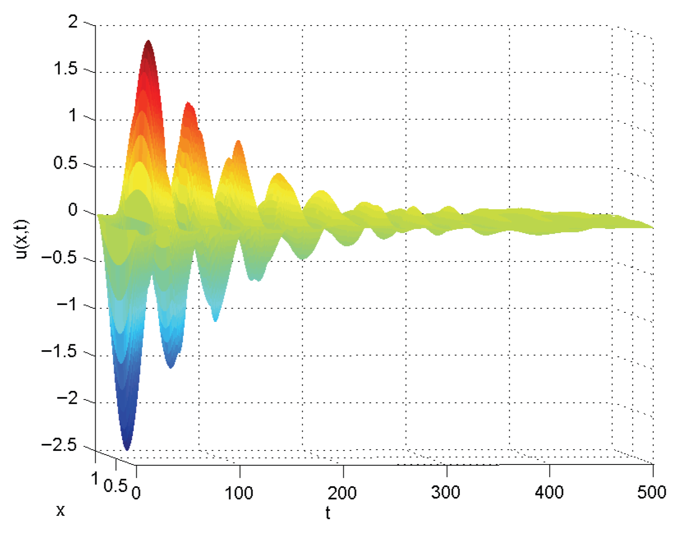
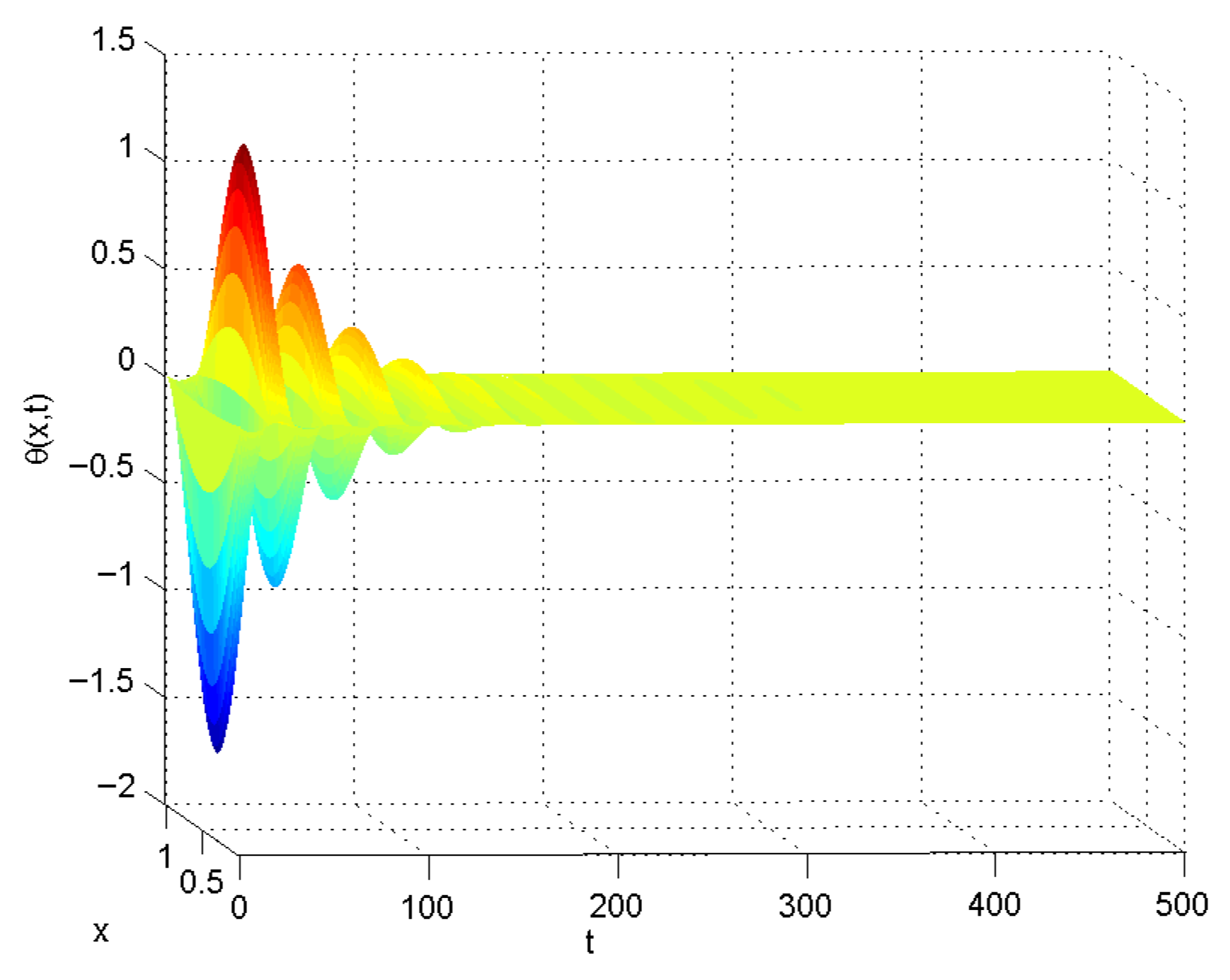
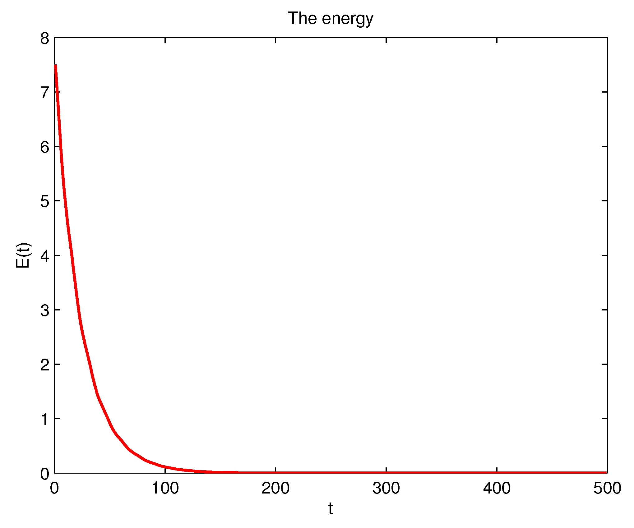
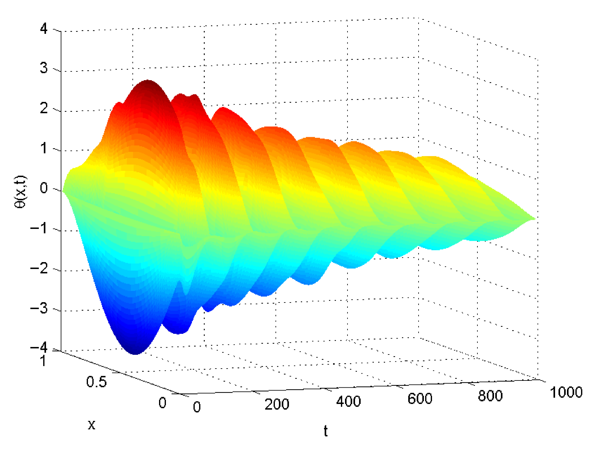
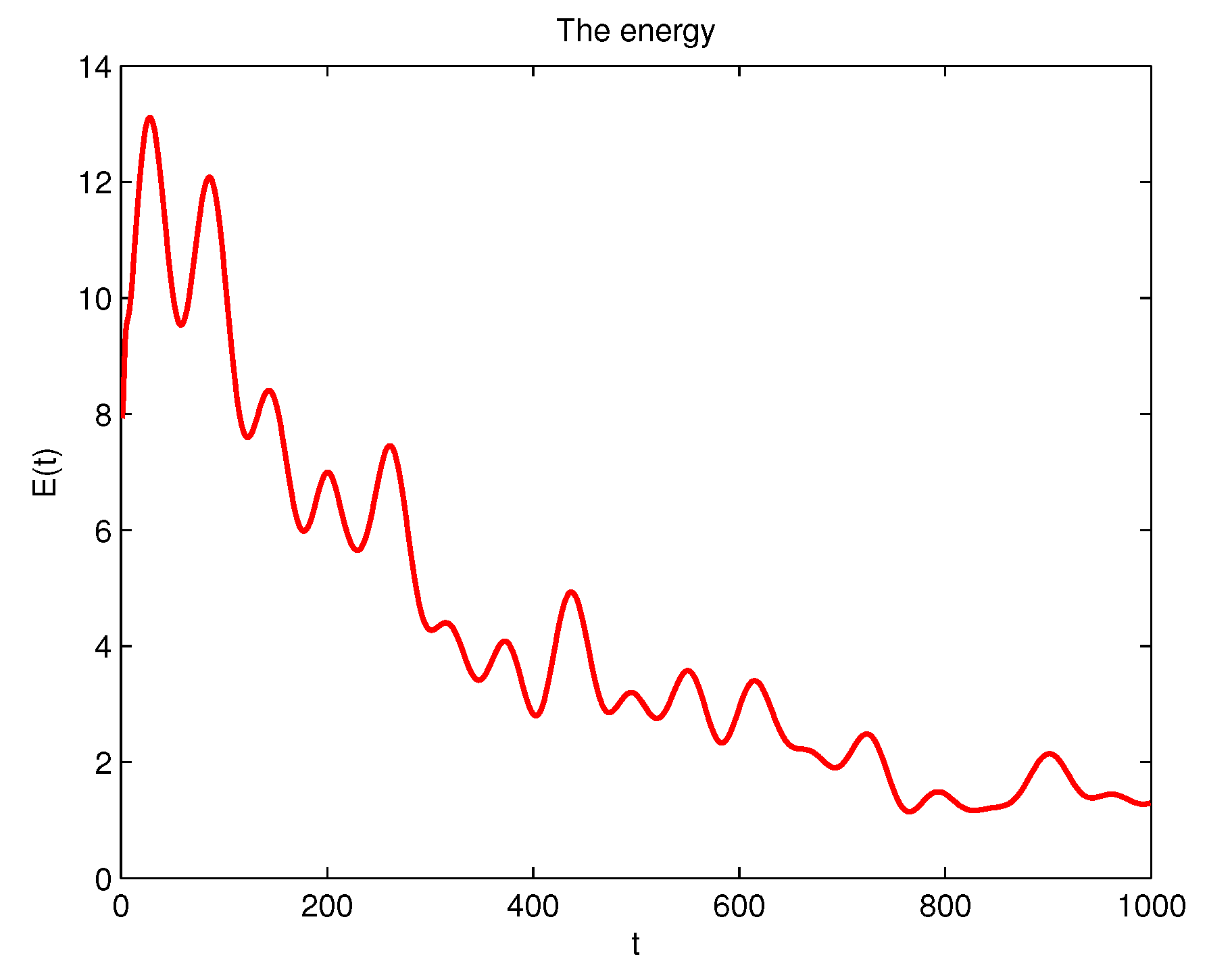
Here is the evolution in time of the solutions $u,$ θ and the discrete energy (Figure 1, Figure 2 and Figure 3).

Example 2.

For the numerical test, we have selected distinct values for the coefficients of the system when (4) holds and (5) does not hold.

$$\rho =7.5,\mu =5.5,\beta =11.5,c=25,\tau =1.5,\kappa =3,{\kappa }^{*}=2.$$

We execute our code using the given discretization parameters: $\mathcal{M}=$ 1000, $\mathcal{N}$$=200$, $l=1$ and $\epsilon ={10}^{-5}$. With the following initial conditions,

$$\begin{array}{cc}\hfill u_0\left(x\right)& ={10}^{-2}\left(x^3-x^2\right),u_1\left(x\right)={\displaystyle \frac{1}{8}}x\left(x-1\right),{\theta }_0\left(x\right)=x^3-{\displaystyle \frac{3}{2}}{x}^2,\hfill \\ \hfill {\theta }_1\left(x\right)& =x^{3}exp\left(-{\displaystyle \frac{3}{2}}{x}^2\right),{\theta }_2\left(x\right)=0.\hfill \end{array}$$

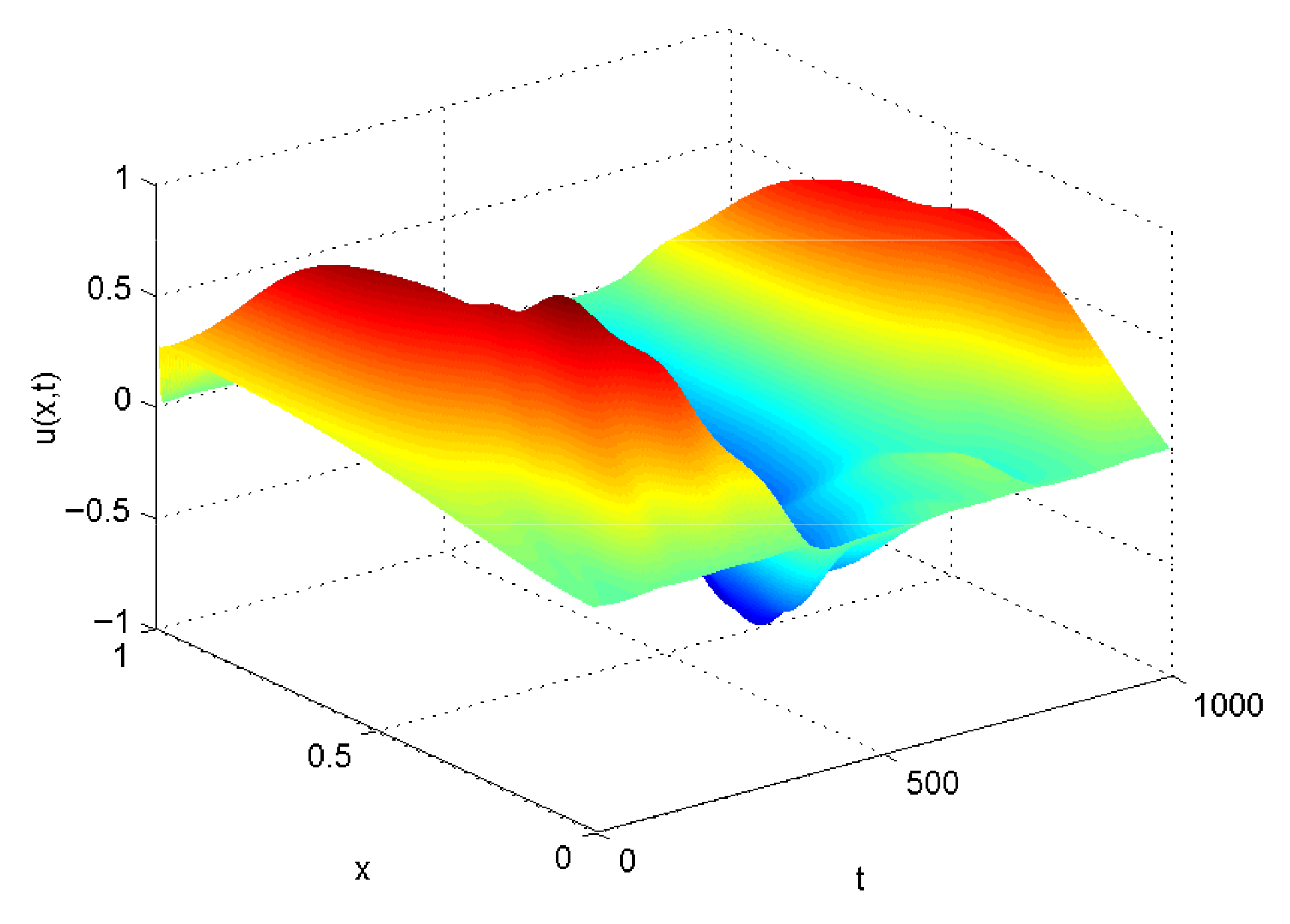
Here is the evolution in time of the solutions $u,$ θ and the discrete energy (Figure 4, Figure 5 and Figure 6):

In the above numerical examples, the graphics presented in Figure 1 and Figure 2 show the evolution in time of the approximation solutions u and $\theta$ in the interval $[0,T]$ for different choices of the system parameters and of the initial data where (4) and (5) hold. Furthermore, Figure 3 shows that the approximate energy (54) decays exponentially, which confirms the main theoretical result obtained. Figure 4 and Figure 5 show the evolution in time where (4) holds and (5) does not hold. Figure 6 confirms that the asymptotic behavior obtained in Example 1 is lacking; additionally, we keep the same initial conditions as in Example 1, and this is illustrated by the theoretical result obtained.

5.3. Numerical Verification: Parameter Study on a Mesh Grid

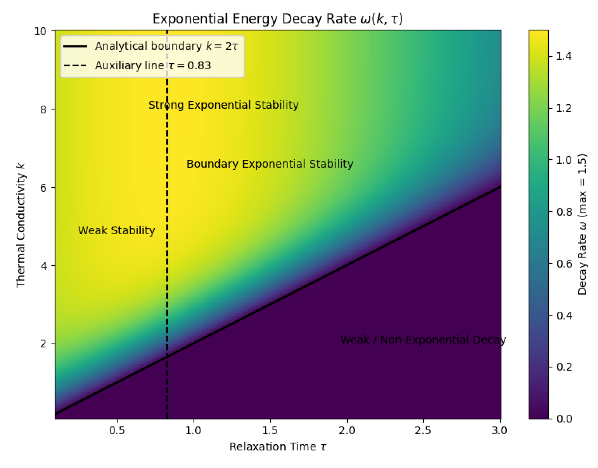
To significantly strengthen the manuscript’s theoretical claims regarding the exponential decay of the energy $E\left(t\right)$ and to move beyond limited illustrative examples, we conducted a comprehensive two-dimensional parameter study on a mesh grid. This approach numerically validates the analytical stability criteria ($\kappa >{\kappa }^{*}\tau$ (3) and $\kappa ={\kappa }^{*}\tau$ with ${\chi }^{\prime }>0$ (4) and (5)) across a vast space of coefficients. The study focuses on mapping the estimated exponential decay rate $\omega$ of the discrete energy functional $E^n\left(t\right)$ (54) as a function of the two critical parameters: $\kappa$ and $\tau$. The resulting behavior map visually confirms the boundaries separating regions of strong exponential stability, boundary exponential stability, and weak/non-exponential decay.

5.3.1. Methodology and Mesh Grid Setup

The numerical verification follows these detailed steps:

• Fixed Parameters: All non-varying system coefficients $(\rho ,\mu ,\beta ,{\kappa }^{★},c)$ are fixed using the values established in the numerical examples (e.g., from Example 1 or 2) to ensure consistency.

  $$\rho =7.5,\mu =5.5,\beta =11.5,c=5.5,{\kappa }^{★}=2$$
• Mesh Grid Definition: A two-dimensional grid is constructed in the $\kappa -\tau$ plane. The domain for the critical parameters is chosen to cover the analytical stability boundaries:

  $$\tau \in [{\tau }_{min},{\tau }_{max}]\mathrm{and}\kappa \in [{\kappa }_{min},{\kappa }_{max}]$$

  with ${\tau }_{min}=0.1,{\tau }_{max}=3,{\kappa }_{min}=0.1,{\kappa }_{max}=10.$
• Discretization and Simulation: For every point $({\kappa }_i,{\tau }_j)$ on the mesh grid, the system is simulated numerically using the discretization scheme (53). The simulation duration ($T_{final}=100$) must be sufficient to ensure the energy reaches its asymptotic decay regime.

5.3.2. Calculation of the Decay Rate $\left(\omega \right)$

For each simulation run, the numerical decay rate is determined by analyzing the recorded values of the discrete energy $E^n\left(t\right)$ (54):

• Energy Tracking: The discrete energy $E^n\left(t\right)$ is calculated at every time step n.
• Linear Fitting: In the long-time regime (where the decay is guaranteed to be exponential, $E\left(t\right)\sim C{e}^{-\omega t}$), the logarithm of the energy is fitted to a straight line: $ln\left(E^n\right)\approx ln\left(C\right)-\omega t_n$.
• Rate Estimation: The exponential decay rate ${\omega }_{i,j}$ for the point $({\kappa }_i,{\tau }_j)$ is defined as the negative of the slope of the fitted line:

  $${\omega }_{i,j}=-\left(\mathrm{Slope}\mathrm{of}\ln \left(\mathrm{E}\right(\mathrm{t})\mathrm{vs}.\mathrm{t}\right)=-\underset{t\to \infty }{lim}{\displaystyle \frac{1}{t}}ln\left(E\left(t\right)\right)$$

5.3.3. Interpretation of the Decay Rate Map

Figure 7 presents the resulting heatmap, where color intensity directly reflects the computed decay rate $\omega$. The value $\omega$ is derived from the linear slope of the $-ln\left(E\right(t\left)\right)$ versus the time curve in the asymptotic regime, where a positive slope confirms exponential stability. The analysis of the map reveals a striking visual confirmation of the theoretical predictions:

• Strong Exponential Stability ($\kappa >2\tau$): The region located above the solid black line ($\kappa =2\tau$) is dominated by the highest $\omega$ values (bright green/yellow colors), which can be seen extending up to $\omega \approx 1.5$. This intense decay rate confirms the strong and fast exponential stability of the system whenever this condition/strong inequality (3) is met, thereby validating the sufficiency of the inequality in Case 1.
• Boundary and Weak Stability: The transition in system behavior is precisely delineated by the analytical critical boundary $\kappa =2\tau$.

  -

  Boundary Stability (Case 2): Points lying directly on the $\kappa =2\tau$ line remain in a region of positive, non-zero $\omega$ (yellow/light green), provided they are to the left of the auxiliary line defined by the secondary condition ${\chi }^{\prime }=0$ (represented by the dashed vertical line $\tau \approx 0.83$). This numerically confirms that the critical line itself represents the limit of exponential stability, not instability.

• Weak/Non-Exponential Decay: The area below the $\kappa =2\tau$ line exhibits $\omega$ values approaching zero (dark red/blue). This validates the necessity of the analytical condition, demonstrating that outside the predicted domain, the exponential decay property is lost, leading to significantly weaker (likely polynomial) or non-existent exponential stability.

Remark 5.

The upper bound Max(ω) = 1.5 corresponds to the maximal exponential decay rate observed in the numerical parameter study. This value reflects the intrinsic saturation of the dissipation mechanism and is consistent with the theoretical boundedness of exponential decay rates in MGT-type thermoelastic systems.

5.3.4. Conclusion on Theoretical Validity

The strong correspondence between the analytically derived stability boundaries and the numerically computed change in the decay rate $\omega$ provides unambiguous evidence of the robustness and accuracy of the theoretical results. The parameter map successfully replaces the need for limited spot checks by comprehensively summarizing the system’s asymptotic behavior across the entire parameter space, fully validating that the derived conditions are both necessary and sufficient for guaranteeing exponential energy decay in the MGT model.

6. Conclusions and Future Work

This work rigorously analyzed the stability of a one-dimensional Moore–Gibson–Thompson (MGT) thermoelastic model incorporating frictional damping. Using semigroup theory, we first established the well posedness of the system and then investigated the exponential stability of the solutions by constructing suitable energy functionals and applying the Lyapunov method. Our theoretical analysis successfully identified the necessary conditions for the exponential decay of the system’s energy, demonstrating that when the combined dissipation (thermal conductivity and frictional damping) is sufficiently strong $\kappa >{\kappa }^{*}\tau$), the system exhibits exponential energy decay; even at the critical threshold of dissipation $\kappa ={\kappa }^{*}\tau$), exponential stability remains achieved, provided a specific parameter balance condition holds. These crucial theoretical results were subsequently confirmed through numerical simulations using finite difference and Euler schemes, which consistently confirmed the predicted exponential decay behavior. To fully validate our analytical findings, our numerical investigation includes a comprehensive parameter analysis. Specifically, we constructed a 2D parameter mesh grid by systematically varying two key system parameters across a wide, relevant range. The results from this study visually and quantitatively confirm the applicability and boundaries of the derived exponential stability conditions, especially the identified critical balance condition. This approach provides compelling and robust evidence to support our broad theoretical claims, confirming the well posedness and stability of the system under diverse operating conditions. Overall, this study emphasizes the vital role of the interplay between thermal relaxation, conductivity, and damping in determining the dynamic behavior of MGT models. As for future work, several directions can now extend this analysis to enhance its physical realism and mathematical depth, paving the way for further investigations in more complex and realistic settings. These directions include extending the stability results to two- and three-dimensional domains for better modeling of real-world structures; incorporating nonlinear damping mechanisms (such as polynomial or fractional damping) and nonlinear boundary conditions to accurately verify their impact on energy decay rates; exploring the system’s stability under non-homogeneous or mixed boundary conditions, such as non-zero temperatures or displacements at the boundaries; generalizing the MGT model to include additional physical properties such as viscoelasticity or variable coefficients; and using more advanced numerical schemes for improved accuracy and efficiency.

References

1. Quintanilla, R. Moore-Gibson-Thompson thermoelasticity with two temperatures. Appl. Eng. Sci. 2020, 1, 100006. [Google Scholar] [CrossRef] [Scilit]
2. Fourier, J.-B.J. Théorie Analytique de la Chaleur; Firmin Didot: Paris, France, 1822. [Google Scholar]
3. Cattaneo, C. On a form of heat equation which eliminates the paradox of instantaneous propagation. C. R. Acad. Sci. Paris 1958, 247, 431–433. [Google Scholar]
4. Lord, H.W.; Shulman, Y. A generalized dunamical theory of thermoelasticity. J. Mech. Phys. Solids. 1967, 15, 299–309. [Google Scholar] [CrossRef] [Scilit]
5. Green, A.E.; Lindsay, K.A. Thermoelasticity. J. Elast. 1972, 2, 1–7. [Google Scholar] [CrossRef] [Scilit]
6. Quintanilla, R. Moore–Gibson–Thompson thermoelasticity. Math. Mech. Solids 2019, 24, 4020–4031. [Google Scholar] [CrossRef] [Scilit]
7. Marin, M.; Öchsner, A.; Bhatti, M.M. Some results inMoore-Gibson-Thompson thermoelasticity of dipolar bodies. Z. Angew. Math. Mech. 2020, 100, e202000090. [Google Scholar] [CrossRef] [Scilit]
8. Fernández, J.R.; Quintanilla, R. Moore-Gibson-Thompson theory for thermoelastic dielectrics. Appl. Math. Mech. Engl. Ed. 2021, 42, 309–316. [Google Scholar] [CrossRef] [Scilit]
9. Raposo, C.A. Rao-Nakra model with internal damping and time delay. Math. Moravica 2021, 25, 53–67. [Google Scholar] [CrossRef] [Scilit]
10. Ailawalia, P.; Marin, M.; Kaur, J. Thermoelastic analysis of a Moore-Gibson-Thompson plate with internal heat source loaded with viscous fluid layers. Acta Mech. 2025, 236, 4823–4835. [Google Scholar] [CrossRef] [Scilit]
11. Hilal, M.I.; Tantawi, R.; Elshazly, I.S.; Halouani, B.; Ailawalia, P.; Lotfy, K. Moore-Gibson-Thompson model for thermal and rational dynamics in microelongated semiconductor solids with gravitational field. AIP Adv. 2025, 15, 035332. [Google Scholar] [CrossRef] [Scilit]
12. Ahmed Yahya, M.H.; Saidi, A.; Abouelregal, A.E.; Zakria, A.; Ahmed, I.E.; Mohammed, F.A. Thermoelastic vibrations for solid cylinder with voids, using Moore-Gibson-Thompson heat conduction model. AIMS Math. 2024, 9, 34588–34605. [Google Scholar] [CrossRef] [Scilit]
13. Ahmed Yahya, M.H.; Zakria, A.; Adam Osman, O.A.; Suhail, M.; Rabih, M.N.A. Fractional Moore–Gibson–Thompson heat conduction for vibration analysis of non-local thermoelastic micro-Beams on a viscoelastic Pasternak foundation. Fractal Fract. 2025, 9, 118. [Google Scholar] [CrossRef] [Scilit]
14. Pellicer, M.; Sola-Morales, J. Optimal scalar products in the Moore-Gibson-Thompson equation. Evol. Equ. Control Theory 2019, 8, 203–220. [Google Scholar] [CrossRef] [Scilit]
15. Bazarra, N.; Fernández, J.R.; Quintanilla, R. Analysis of a Moore-Gibson-Thompson thermoelastic problem. J. Comput. Appl. Math. 2021, 382, 113058. [Google Scholar] [CrossRef] [Scilit]
16. Abouelregal, A.E.; Ahmad, H.; Nofal, T.A.; Abu-Zinadah, H. Moore-Gibson-Thompson thermoelasticity model with temperature dependent properties for thermo-viscoelastic orthotropic solid cylinder of infinite length under a temperature pulse. Phys. Scr. 2021, 96, 105201. [Google Scholar] [CrossRef] [Scilit]
17. Abouelregal, A.E.; Akgöz, B.; Civalek, Ö. Magneto-thermoelastic interactions in an unbounded orthotropic viscoelastic solid under the Hall current effect by the fourth-order Moore-Gibson-Thompson equation. Comput. Math. Appl. 2023, 141, 102–115. [Google Scholar] [CrossRef] [Scilit]
18. Abouelregal, A.E.; Dassios, I.; Moaaz, O. Moore–Gibson–Thompson thermoelastic model effect of laser-induced microstructures of a microbeam sitting on visco-pasternak foundations. Appl. Sci. 2022, 12, 9206. [Google Scholar] [CrossRef] [Scilit]
19. Adel, M.; El-Dali, A.; Seddeek, M.A.; Yahya, A.S.; El-Bary, A.A.; Lotfy, K. The Fractional Derivative and Moisture Diffusivity for Moore-Gibson-Thompson Model of Rotating Magneto-Semiconducting Material. J. Vib. Eng. Technol. 2024, 12, 233–249. [Google Scholar] [CrossRef] [Scilit]
20. Apalara, T.A. Exponential decay in one-dimensional porous dissipation elasticity. Q. J. Mech. Appl. Math. 2017, 70, 363–372. [Google Scholar] [CrossRef] [Scilit]
21. Mesmouli, M.B.; Khochemane, H.E. Theoretical study and numerical test for a delayed thermoelastic porous system with microtemperatures. Z. Angew. Math. Mech. 2025, 105, e202400123. [Google Scholar] [CrossRef] [Scilit]
22. Messaoudi, H.; Zitouni, S.; Khochemane, H.E.; Ardjouni, A. General stability for piezoelectric beams with a nonlinear damping term. Ann. Dell’Universita’ Di Ferrara 2023, 69, 443–462. [Google Scholar] [CrossRef] [Scilit]
23. Liu, Z.; Zheng, S. Semigroup Associated with Dissipative System, Research Notes in Mathematics; Chapman & Hall/CRC: Boca Raton, FL, USA, 1999; Volume 398. [Google Scholar]
24. Pazy, A. Semigroups of Linear Operators and Applications to Partial Differential Equations; Springer: New York, NY, USA, 1983. [Google Scholar]
Figure 1. Evolution in time of u.
Mathematics 14 00117 g001
Figure 2. Evolution in time of θ .
Mathematics 14 00117 g002
Figure 3. Evolution in time of E n .
Mathematics 14 00117 g003
Figure 4. Evolution in time of the function u.
Mathematics 14 00117 g004
Figure 5. Evolution in time of the function θ .
Mathematics 14 00117 g005
Figure 6. Evolution in time of the discrete energy.
Mathematics 14 00117 g006
Figure 7. Exponential energy decay rate and stability regions.
Mathematics 14 00117 g007