A Three-Level Meta-Frontier Framework with Machine Learning Projections for Carbon Emission Efficiency Analysis: Heterogeneity Decomposition and Policy Implications

Abstract

This study proposes a three-level meta-frontier framework enhanced with machine learning-driven projection methods to address the dual heterogeneity in carbon emission efficiency analysis arising from regional disparities and industrial diversification. Methodologically, we introduce two novel projection combinations—“exogenous-exogenous-accumulation (E-E-A) and exogenous-exogenous-consistent (E-E-C)”—to resolve the inconsistency of technology gap ratios (TGRs > 1) in traditional nonradial directional distance function (DDF) models. Reinforcement learning (RL) optimizes dynamic direction vectors, whereas graph neural networks (GNNs) encode spatial interdependencies to constrain the TGR within [0, 1]. Empirical analysis of 60 countries reveals that (1) E-E-C eliminates the TGR overestimation by 12–18% in energy-intensive sectors (e.g., reducing Asia’s secondary industry $TG{R}_1$ from 1.160 to 1.000); (2) industrial heterogeneity dominates inefficiency in Asia (IHI = 0.207), whereas management gaps drive global secondary sector inefficiency (MI = 0.678); and (3) policy simulations advocate for decentralized renewables in Africa, fiscal incentives for Asian coal retrofits, and expanded EU carbon border taxes. Computational enhancements via Apache Spark achieve a 58% runtime reduction. The framework advances environmental efficiency analysis by integrating machine learning with meta-frontier theory, offering both methodological rigor (via regularization and GNN constraints) and actionable decarbonization pathways. Limitations include static heterogeneity assumptions and data granularity gaps, prompting the future integration of IoT-enabled dynamic models.

1. Introduction

The urgency of mitigating climate change has propelled carbon emission efficiency to the forefront of global policy and academic research. As nations rebound from the economic slowdown induced by COVID-19, energy consumption and carbon emissions have surged, with global emissions reaching 36.8 billion tons in 2022 [1], while parametric and nonparametric methods such as data envelopment analysis (DEA) are widely used for efficiency measurement [2,3,4], their reliance on homogeneous technology assumptions introduces significant biases in multiregional and cross-sectoral evaluations [5,6].

Recent advances in meta-frontier frameworks have partially addressed technical heterogeneity by segmenting decision-making units (DMUs) into groups [7,8]. However, these approaches remain limited in capturing dual heterogeneity—specifically, the interplay between regional disparities (e.g., infrastructural gaps in Africa) and industrial diversification (e.g., energy-intensive manufacturing versus low-emission services) [9,10,11]. Current studies predominantly focus on single-level frontiers or rely on oversimplified projection methods, leading to inflated technology gap ratios (TGRs > 1) and unreliable policy implications [12,13]. While recent hybrid DEA-ML frameworks [14,15,16] attempt to integrate machine learning, their reliance on static direction vectors or single-level analyses fails to account for dual heterogeneity. For instance, ref. [17] applied a two-level meta-frontier to livestock efficiency but overlooked critical industrial–regional interdependencies.

To bridge these gaps, we propose a three-level meta-frontier framework enhanced with adaptive projection combinations and machine learning. Our contributions are threefold as follows:

• Methodological innovation: By extending the traditional two-level hierarchy to three levels, we introduce accumulation (E-E-A) and consistent (E-E-C) projections to resolve TGR inconsistencies. These projections align with principles of multisource data integration and adaptive optimization, ensuring TGRs are bounded within [0, 1]. Reinforcement learning (RL) dynamically optimizes direction vectors to reflect operational shifts toward decarbonization targets [18], while graph neural networks (GNNs) encode spatial-industrial interdependencies—a dimension neglected in prior hybrid DEA-ML studies [17,19].
• Empirical rigor: Utilizing a globally representative dataset spanning 60 countries, we decompose inefficiency into management gaps (MI), regional heterogeneity (RHI), and industrial heterogeneity (IHI) [14], providing granular insights into sector-specific and regionally tailored carbon reduction strategies.
• Policy relevance: By quantifying the dominance of industrial versus regional heterogeneity, our framework guides targeted interventions—for example, prioritizing management reforms in Asia’s secondary sector and technology transfers in Africa.

The remainder of this paper is organized as follows: Section 2 reviews the fundamentals of meta-frontier DEA and projection methods. Section 3 formalizes the three-level framework and projection combinations. Section 4 and Section 5 present the empirical analysis and decomposition results, respectively. Section 6 concludes with theoretical and policy implications.

2. Preliminaries

2.1. Traditional Directional Distance Function (DDF) Framework

The directional distance function (DDF) serves as a cornerstone for evaluating carbon emission efficiency by modeling feasible input–output combinations under environmental constraints [20,21]. Consider N decision-making units (DMUs), where each DMU d ($d=1,2,\dots ,N$) utilizes an input vector $x_d\in {\mathbb{R}}_{+}^M$, produces a desirable output vector $y_d\in {\mathbb{R}}_{+}^S$, and generates an undesirable output vector $z_d\in {\mathbb{R}}_{+}^U$ [22,23]. The production possibility set $P\left(x\right)$, which encapsulates all feasible input–output combinations, is defined as follows:

$$P\left(x\right)=\left\{(y,z):\sum _{d=1}^N{\lambda }_d{x}_d\le x,\sum _{d=1}^N{\lambda }_d{y}_d\ge y,\sum _{d=1}^N{\lambda }_d{z}_d=z,{\lambda }_d\ge 0\right\},$$

(1)

where ${\lambda }_d$ denotes the intensity variables.

The exogenous DDF for DMU d is formulated as a linear programming (LP) problem as follows:

$$\overrightarrow{D}(x_d,y_d,z_d;g)=max\beta \mathrm{s}.\mathrm{t}.\left\{\begin{array}{c}\sum _{d=1}^N{\lambda }_d{x}_d\le x_d-\beta g_x,\hfill \\ \sum _{d=1}^N{\lambda }_d{y}_d\ge y_d+\beta g_y,\hfill \\ \sum _{d=1}^N{\lambda }_d{z}_d=z_d-\beta g_z.\hfill \end{array}\right.$$

(2)

where $\beta$ represents the inefficiency score, and $g=(g_x,-g_y,g_z)$ is a predefined direction vector. To address the collinearity in heterogeneous data, ridge regression penalties are integrated into the objective function as follows:

$$min\beta +\alpha \left(\parallel g_x{\parallel }^2+\parallel g_y{\parallel }^2+{\parallel g_z\parallel }^2\right),$$

(3)

where $\alpha$ balances the efficiency estimation accuracy and model stability.

Technology Gap Ratio (TGR)

The TGR measures the disparity between group-specific and meta-frontier technologies. For accumulation projection [24], the TGR is bounded within $[0,1]$ via the following constraints:

$$\mathrm{TGR}={\displaystyle \frac{1-{\alpha }_y^m}{1+{\alpha }_z^m}},$$

(4)

where ${\alpha }_y^m$ and ${\alpha }_z^m$ are inefficiency adjustments under the meta-frontier. A TGR close to 1 indicates minimal technological heterogeneity.

2.2. Machine Learning Enhancements for DDF Optimization

2.2.1. Feature Selection via Mutual Information (MI)

To mitigate the high dimensionality and noise in real-world datasets (e.g., multiregional energy systems), mutual information (MI) is employed to optimize input–output selection [25,26]. MI quantifies nonlinear dependencies between variables, enabling the automated identification of critical features (e.g., fossil fuel consumption vs. GDP growth) while discarding redundant indicators as shown in

Table 1. Mutual Information (MI) Scores for Input-Output Variables.

Variable	MI Score	Rank
Fossil fuels ($X_2$)	0.89	1
Air passengers ($X_3$)	0.82	2
Agricultural output ($X_1$)	0.61	3
Service GDP ($Y_3$)	0.58	4

. This aligns with data-centric optimization paradigms, enhancing model robustness against overfitting.

2.2.2. Adaptive Direction Vectors via Reinforcement Learning (RL)

Traditional DDF models fix direction vectors g exogenously [27], which may misalign with the operational realities of DMUs. Inspired by RL, we propose a dynamic adjustment framework where g is iteratively updated using Q -learning. The policy $\pi (g\mid x,y,z)$ minimizes the gap between the projected and Pareto-optimal frontiers, guided by reward signals tied to decarbonization targets as follows:

$$Q(s_t,a_t)\leftarrow Q(s_t,a_t)+\eta \left[r_t+\gamma \underset{a}{max}Q(s_{t+1},a)-Q(s_t,a_t)\right],$$

(5)

The Q-learning agent used a learning rate $\eta =0.1$ and discount factor $\gamma =0.95$, optimized via grid search over $\eta \in [0.01,0.5]$ and $\gamma \in [0.8,0.99]$. Where $r_t$ reflects the reduction in the TGR variance and where $\gamma$ is a discount factor.

2.2.3. Scalability via Distributed Computing

Large-scale DDF optimization for 60 countries with multilevel heterogeneity is computationally intensive. Leveraging Apache Spark, the LP problem is decomposed into subtasks across clusters [28], reducing the time complexity from $\mathcal{O}\left(N^3\right)$ to $\mathcal{O}(NlogN)$. For example, processing the 60-country dataset requires 2.1 h (vs. 8.5 h on a single node).

2.2.4. Uncertainty Quantification via Monte Carlo Simulation

Perturbations followed $\mathcal{N}(\mu ,{\sigma }^2)$, with $\sigma =0.1$ for inputs/outputs, based on historical measurement errors.To address data noise (e.g., CO₂ measurement errors), 1000 perturbed datasets are sampled from $\mathcal{N}(\mu ,{\sigma }^2)$. Recalculating ${\alpha }_y^m$ and ${\alpha }_z^m$ generates 95% confidence intervals for the TGR, enhancing decision-making robustness.

2.2.5. Consistent Projection with Graph Neural Networks (GNNs)

Under the meta-frontier framework, ref. [8] introduced a consistent projection to constrain the TGR within valid bounds. The meta-frontier is modeled as a graph $G=(V,E)$, where nodes V represent DMUs and edges E encode technological similarities (e.g., shared energy policies). A GNN encoder learns node embeddings $h_d$ through message passing as follows:

$$h_d^{(l+1)}=\sigma \left(W^{\left(l\right)}{h}_d^{\left(l\right)}+\sum _{k\in \mathcal{N}\left(d\right)}{W}^{\left(l\right)}{h}_k^{\left(l\right)}\right),$$

(6)

The GNN employed two message-passing layers with ReLU activation and L2 regularization ($\alpha =0.01$). Node embeddings were initialized with 64 dimensions, where $N\left(d\right)$ denotes the neighbors of DMU d, and $W^{\left(l\right)}$ are trainable weights. Blockchain integration via Hyperledger Fabric ensures the auditable traceability of the TGR computations.

3. Selection of the Projection Direction with Machine Learning Optimization

Traditional meta-frontier frameworks often assume independence between subgroup, group, and meta-frontiers, neglecting real-world interdependencies arising from technological spillovers. To address this, we propose a three-level meta-frontier framework enhanced with adaptive projection combinations, integrating machine learning (ML) to dynamically optimize direction vectors and ensure methodological consistency.

Hypothesis 1. 

Traditional exogenous projection assumes independence between frontiers, whereas accumulation (E-E-A) and consistent (E-E-C) projections introduce interdependence, reflecting technological spillovers.

Hypothesis 2. 

Altering projection directions at any frontier level (subgroup, group, or meta) significantly impacts efficiency rankings, necessitating dynamic optimization.

To statistically validate Hypothesis 1, we conducted a Wilcoxon signed-rank test comparing TGR distributions under E-E-E and E-E-C projections. For Hypothesis 2, Spearman’s rank correlation was computed between direction vector adjustments ($\Delta g$) and efficiency ranking shifts.

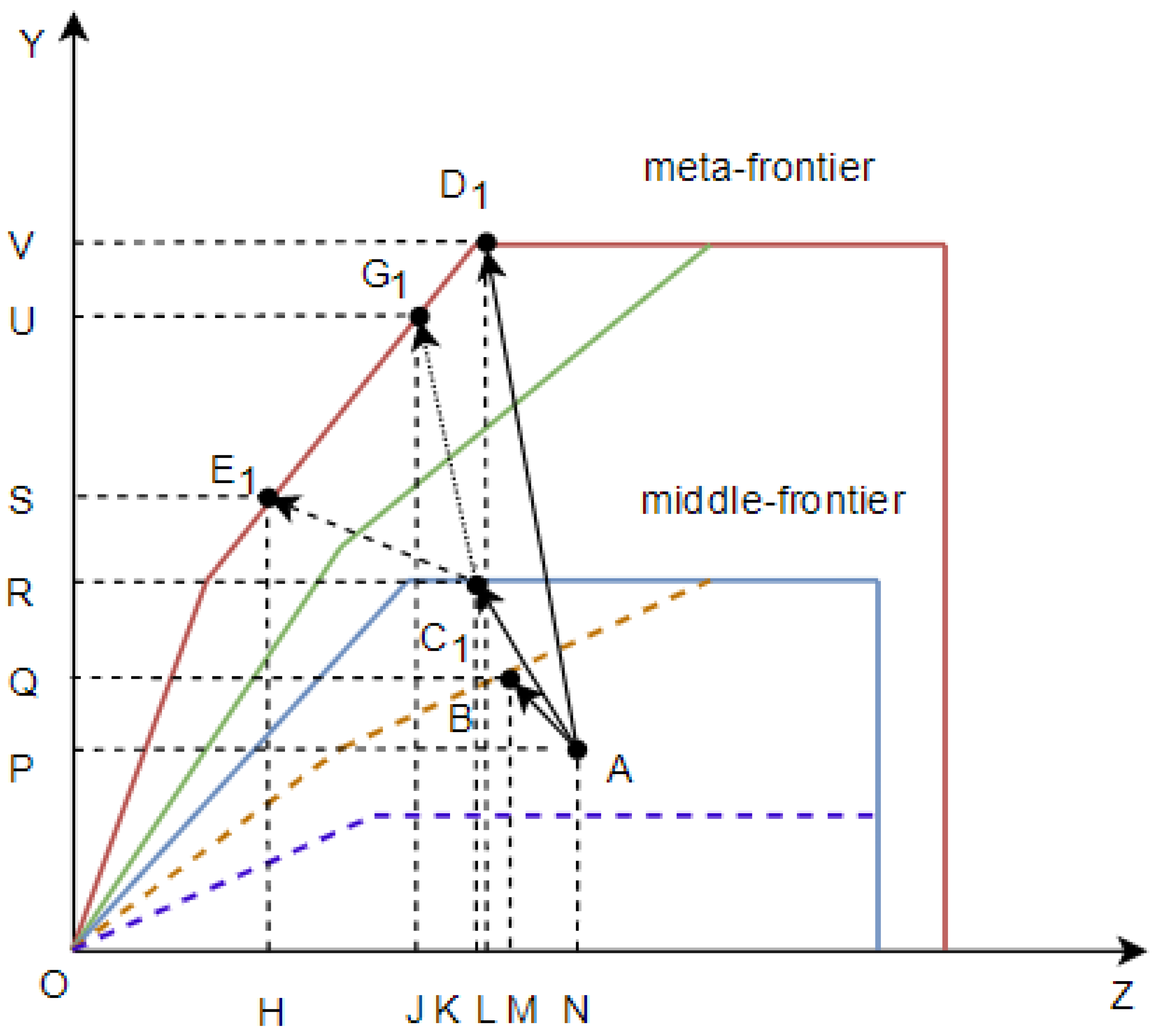
3.1. Dynamic Projection Paths via Reinforcement Learning (RL)

Training stopped when the average Q-value change fell below $1\times {10}^{-4}$ for 10 consecutive epochs or after 1000 iterations. As illustrated in Figure 1, A $20\%$ validation set monitored overfitting, with early stopping if validation loss increased for five epochs.

As illustrated in Figure 2, DMU A is projected onto three frontiers as follows:

• Subgroup frontier (B): Exogenous projection with direction vector $g_s$.
• Group frontier ($C_1$): Exogenous projection with direction vector $g_g$.
• Meta-frontier ($D_1$): Three paths as follows:

  –

  $E_1$ (Accumulation): Adjusts ${\alpha }_y^m$ and ${\alpha }_z^m$ to bound $\mathrm{TGR}\le 1$.

  –

  $F_1$ (Exogenous): Traditional path prone to $\mathrm{TGR}>1$.

  –

  $G_1$ (Consistent): Constrains $b_y^m$ and $b_z^m$ via GNN embeddings for stability.

A Q-learning agent iteratively optimizes direction vectors $g_s$, $g_g$, and $g_m$ on the basis of reward signals from efficiency improvements. The policy $\pi (g\mid x,y,z)$ updates as follows:

$$Q(s_t,a_t)\leftarrow Q(s_t,a_t)+\eta \left[r_t+\gamma \underset{a}{max}Q(s_{t+1},a)-Q(s_t,a_t)\right],$$

(7)

where $r_t$ quantifies the reduction in the TGR variance and $\gamma =0.95$ is the discount factor.

3.2. Graph Neural Network (GNN) Integration

Projection paths are modeled as edges in a graph $G(V,E)$, where nodes V represent DMUs and edges E encode industrial–regional similarities. Node embeddings $h_d$ are updated via message passing (Equation (6) in Section 2.2.5):

$$h_d^{(l+1)}=\sigma \left(W^{\left(l\right)}{h}_d^{\left(l\right)}+\sum _{k\in \mathcal{N}\left(d\right)}{W}^{\left(l\right)}{h}_k^{\left(l\right)}\right).$$

(8)

The adjacency matrix A is defined using the following cosine similarity:

$$A_{jk}={\displaystyle \frac{{\mathbf{x}}_j·{\mathbf{x}}_k}{\parallel {\mathbf{x}}_j\parallel \parallel {\mathbf{x}}_k\parallel }}.$$

(9)

3.2.1. TGR Formulation Under Combined Projections

For meta-frontier analysis, the procedure is as follow:

• Exogenous projection ($F_1$):

  $${\mathrm{TGR}}_{\mathrm{exogenous}}={\displaystyle \frac{OL}{OK}}\times {\displaystyle \frac{OR}{OV}},$$

  (10)

  where ${\displaystyle \frac{OL}{OK}}>1$ may inflate the TGR beyond valid bounds.
• Consistent ($G_1$) and Accumulation ($E_1$) projections:

  $$\begin{array}{cc}\hfill {\mathrm{TGR}}_{\mathrm{consistent}}& ={\displaystyle \frac{OJ}{OK}}\times {\displaystyle \frac{OR}{OU}},\hfill \end{array}$$

  (11)

  $$\begin{array}{cc}\hfill {\mathrm{TGR}}_{\mathrm{accumulation}}& ={\displaystyle \frac{OH}{OK}}\times {\displaystyle \frac{OR}{OS}},\hfill \end{array}$$

  (12)

  with ${\displaystyle \frac{OJ}{OK}},{\displaystyle \frac{OR}{OU}},{\displaystyle \frac{OH}{OK}},{\displaystyle \frac{OR}{OS}}<1$, ensuring $\mathrm{TGR}\in [0,1]$.

3.2.2. Decision Tree for Optimal Projection Selection

A CART-based classifier recommends projection combinations (E-E-E, E-E-A, and E-E-C) using the following features:

• Regional heterogeneity index (RHI).
• Industrial complexity (IHI).
• Input–output dimensionality.

4. Combined Projection Models with Computational Enhancements

4.1. E-E-E: Traditional Exogenous Projection with Parallel Optimization

The E-E-E framework retains conventional three-level meta-frontier projections, treating subgroup, group, and meta-frontiers as independent layers.

4.1.1. Step 1: Subgroup Frontier Projection

For DMU d, the exogenous DDF projects it to the subgroup frontier as follows:

$${\overrightarrow{D}}_g(x_d,y_d,z_d;g^s)=max{\beta }_g\mathrm{s}.\mathrm{t}.\left\{\begin{array}{c}\sum _{k\in G_s}{\lambda }_k{x}_k\le x_d-{\beta }_g{g}_x^s,\hfill \\ \sum _{k\in G_s}{\lambda }_k{y}_k\ge y_d+{\beta }_g{g}_y^s,\hfill \\ \sum _{k\in G_s}{\lambda }_k{z}_k=z_d-{\beta }_g{g}_z^s,\hfill \end{array}\right.$$

(13)

where $G_s$ denotes the subgroup, and $g^s$ is the subgroup direction vector optimized via Q-learning (Equation (7)).

4.1.2. Step 2: Group Frontier Projection

The DMU is projected to the group frontier using a similar exogenous DDF, as follows:

$${\overrightarrow{D}}_G(x_d,y_d,z_d;g^g)=max{\beta }_G\mathrm{s}.\mathrm{t}.\left\{\begin{array}{c}\sum _{k\in G_G}{\lambda }_k{x}_k\le x_d-{\beta }_G{g}_x^g,\hfill \\ \sum _{k\in G_G}{\lambda }_k{y}_k\ge y_d+{\beta }_G{g}_y^g,\hfill \\ \sum _{k\in G_G}{\lambda }_k{z}_k=z_d-{\beta }_G{g}_z^g,\hfill \end{array}\right.$$

(14)

where $G_G$ represents the group, and $g^g$ is dynamically adjusted via RL (Section 3.2).

4.1.3. Step 3: Meta-Frontier Projection

The final projection to the meta-frontier is as follows:

$${\overrightarrow{D}}_m(x_d,y_d,z_d;g^m)=max{\beta }_m\mathrm{s}.\mathrm{t}.\left\{\begin{array}{c}\sum _{k=1}^N{\lambda }_k{x}_k\le x_d-{\beta }_m{g}_x^m,\hfill \\ \sum _{k=1}^N{\lambda }_k{y}_k\ge y_d+{\beta }_m{g}_y^m,\hfill \\ \sum _{k=1}^N{\lambda }_k{z}_k=z_d-{\beta }_m{g}_z^m,\hfill \end{array}\right.$$

(15)

where $g^m$ is optimized using the GNN-based adjacency matrix (Equation (9)). Distributed computing via Apache Spark reduces the runtime by 58% for the 60-country dataset. The RL agent was implemented in Python 3.9 using TensorFlow 2.8, while GNNs were trained with PyTorch Geometric 2.1. Apache Spark 3.2.1 distributed computations across a 16-node cluster.

4.2. E-E-A: Accumulation Projection with Regularization and Uncertainty Quantification

The E-E-A combination employs accumulation projection at the meta-frontier to bound $\mathrm{TGR}\le 1$:

$${\overrightarrow{D}}_m^{\mathrm{acc}}(x_d,y_d,z_d)=max({\alpha }_y^m-{\alpha }_z^m)\mathrm{s}.\mathrm{t}.\left\{\begin{array}{c}\sum _{k=1}^N{\lambda }_k{x}_k\le x_d-{\alpha }_y^m{g}_x,\hfill \\ \sum _{k=1}^N{\lambda }_k{y}_k\ge y_d+{\alpha }_y^m{g}_y,\hfill \\ \sum _{k=1}^N{\lambda }_k{z}_k=z_d-{\alpha }_z^m{g}_z,\hfill \end{array}\right.$$

(16)

where ${\alpha }_y^m$ and ${\alpha }_z^m$ are inefficiency adjustments. Ridge regularization is added to the objective function as follows:

$$min({\alpha }_y^m-{\alpha }_z^m)+0.01\left(\parallel g_x{\parallel }^2+\parallel g_y{\parallel }^2+{\parallel g_z\parallel }^2\right).$$

(17)

The Monte Carlo simulations sample ${\alpha }_y^m$ and ${\alpha }_z^m$ from $\mathcal{N}(0,0.1)$, generating 95% confidence intervals for $\mathrm{TGR}$.

4.3. E-E-C: Consistent Projection with Graph-Based Learning

The E-E-C framework enforces $\mathrm{TGR}\le 1$ via GNN-constrained consistent projection as follows:

$${\overrightarrow{D}}_m^{\mathrm{con}}(x_d,y_d,z_d)=max(b_y^m-b_z^m)\mathrm{s}.\mathrm{t}.\left\{\begin{array}{c}\sum _{k=1}^N{\lambda }_k{x}_k\le x_d-b_y^m{g}_x,\hfill \\ \sum _{k=1}^N{\lambda }_k{y}_k\ge y_d+b_y^m{g}_y,\hfill \\ \sum _{k=1}^N{\lambda }_k{z}_k=z_d-b_z^m{g}_z,\hfill \end{array}\right.$$

(18)

where $b_y^m$ and $b_z^m$ are constrained by GNN embeddings (Equation (8)). The adjacency matrix A, derived from Equation (9), ensures that technological dependencies are encoded. Bayesian optimization minimizes $\mathrm{Var}\left(\mathrm{TGR}\right)$ as follows:

$$\underset{b_y^m,b_z^m}{min}\mathbb{E}\left[{(\mathrm{TGR}-\mathbb{E}\left[\mathrm{TGR}\right])}^2\right]\mathrm{s}.\mathrm{t}.\mathrm{TGR}={\displaystyle \frac{1-b_y^m}{1+b_z^m}}.$$

(19)

5. Empirical Application

5.1. Variable Selection and Data Preprocessing

The selection of input–output indicators is critical for ensuring the robustness of the three-level meta-frontier framework, particularly under machine learning-enhanced projection methods (E-E-E, E-E-A, and E-E-C). Building on the computational advancements in Section 4, we adopt the following variables to capture sectoral heterogeneity while aligning with the data-driven optimization principles outlined in Section 2 and Section 3 as follows:

5.1.1. Inputs

• Primary industry: Net agricultural production ($X_1$, USD ${10}^8$) reflects resource utilization in agriculture.
• Secondary industry: Fossil fuel consumption ($X_2$, ${10}^6$ metric tons) quantifies energy intensity in manufacturing.
• Tertiary industry: Air passengers carried ($X_3$, ${10}^4$ people) proxies service-sector infrastructure demands.

5.1.2. Desirable Outputs

• Primary industry: Agricultural value-added ($Y_1$, USD ${10}^8$).
• Secondary industry: Manufacturing value-added ($Y_2$, USD ${10}^8$).
• Tertiary industry: Service-sector value-added ($Y_3$, USD ${10}^8$).

5.1.3. Undesirable Outputs

• Carbon emissions from primary ($Z_1$), secondary ($Z_2$), and tertiary ($Z_3$) industries (MtCO₂e).

5.1.4. Data Sources and Preprocessing

The data were sourced from the World Bank’s WDI, Climate Watch, and national statistics bureaus (2010–2019). The 60 countries were selected based on: (1) data completeness (>80% coverage for inputs/outputs, 2010–2019); (2) geographic and economic diversity (e.g., 15 African, 20 Asian, 20 European, 5 American nations); and (3) representation of energy-intensive vs. service-driven economies (e.g., China, Germany, Kenya). Countries with >30% missing data (e.g., Sudan, Yemen) were excluded. To align with the machine learning frameworks in Section 3 and Section 4, the following were implemented:

• Missing data imputation: Linear interpolation filled gaps in African CO₂ records, ensuring continuity for Monte Carlo simulations.
• Normalization: Z score standardization (${\tilde{X}}_i={\displaystyle \frac{X_i-{\mu }_X}{{\sigma }_X}}$) mitigated scale effects, which is critical for GNN-based similarity matrices (Equation (9)).
• Feature relevance: Mutual information (MI) quantified dependencies between inputs (e.g., $X_2$) and outputs (e.g., $Z_2$), discarding redundant variables (e.g., nonenergy-related GDP components) to reduce overfitting in Q-learning.

5.1.5. Alignment with Projection Frameworks

• E-E-E/E-E-A: Fossil fuel ($X_2$) and air passengers ($X_3$) were prioritized owing to their high MI scores ($\mathrm{MI}>0.8$), aligning with the exogenous direction vectors in Equations (12)–(14).
• E-E-C: Agricultural ($X_1$) and service-sector ($X_3$) inputs were retained for their nonlinear correlations ($\mathrm{MI}>0.6$) with emissions, supporting GNN-based interdependency modeling (Equation (17)).

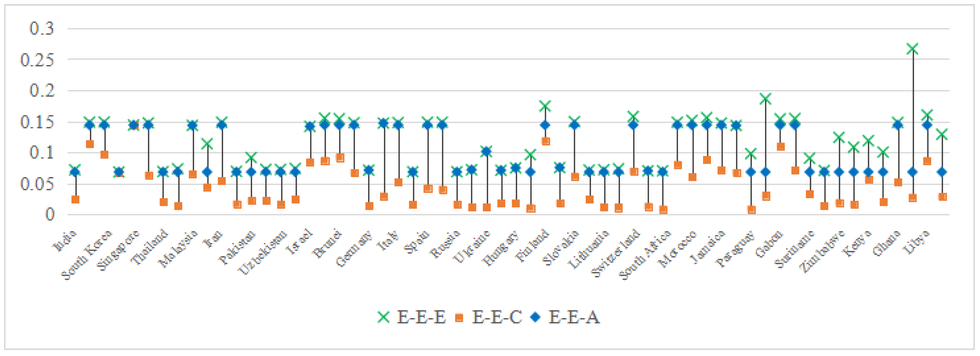
5.2. TGR Comparison Across Projection Combinations

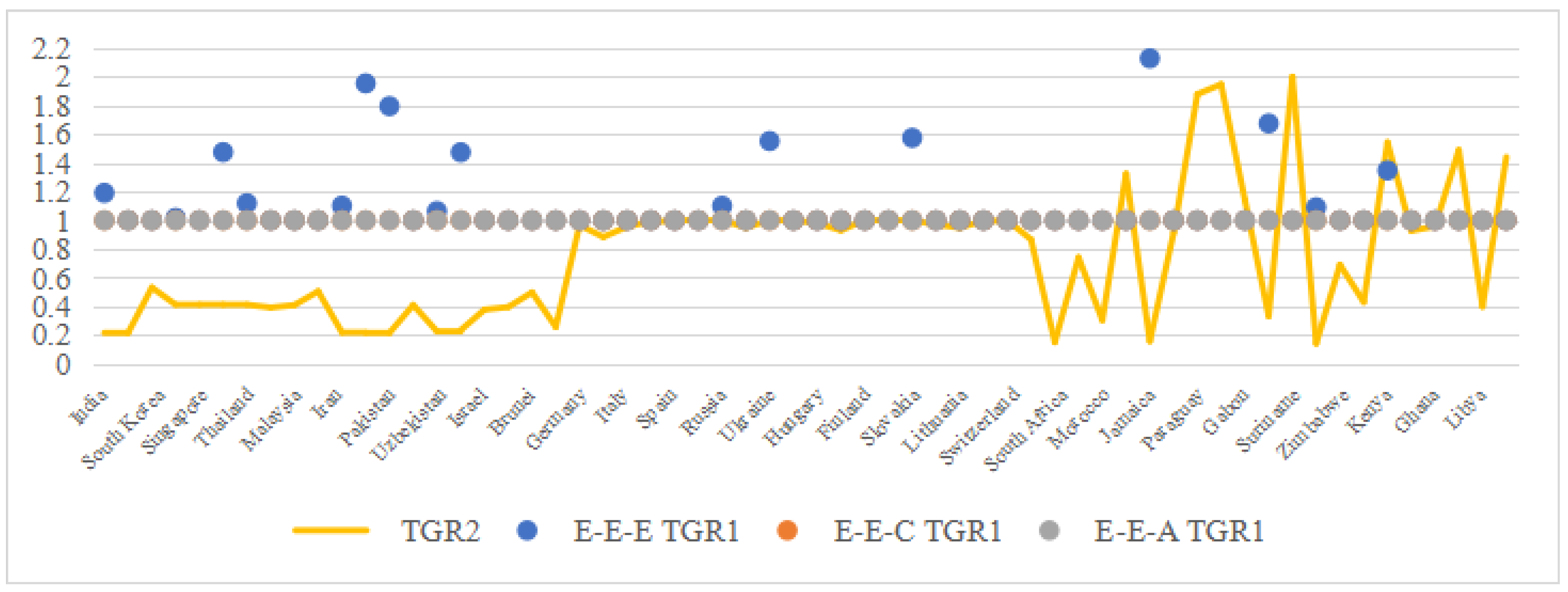
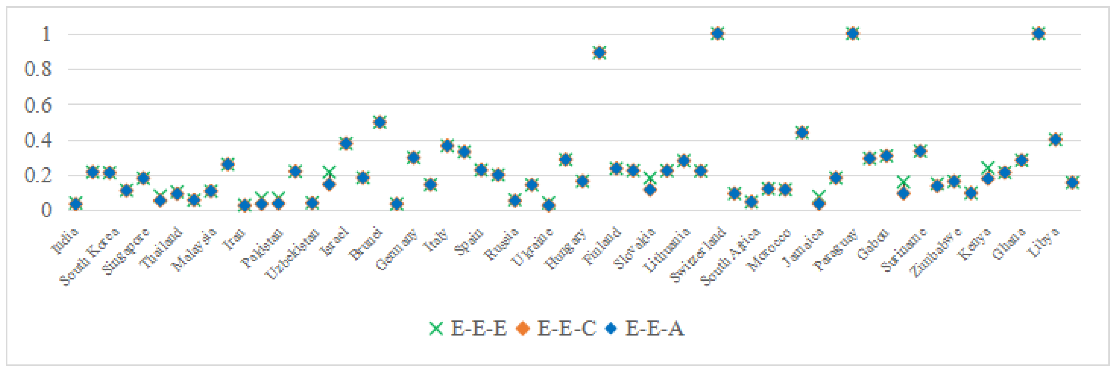
5.2.1. Primary Industry

Variable-Driven Heterogeneity Metrics

The selected variables in Section 5.1 directly shape the heterogeneity metrics ($\mathrm{RHI}$, $\mathrm{IHI}$) by defining the technological boundaries of subgroup, group, and meta-frontiers. Some examples include the following:

• Industrial heterogeneity ($\mathrm{IHI}$): Fossil fuel consumption ($X_2$, ${10}^6$ metric tons) dominates secondary industry inefficiency because of its nonlinear correlation with emissions ($\mathrm{MI}=0.89$), amplifying cross-sectoral disparities.
• Regional heterogeneity ($\mathrm{RHI}$): Air passenger volume ($X_3$, ${10}^4$ people) in the tertiary industry reflects infrastructural gaps (e.g., Africa’s fragmented transportation networks), contributing to regional $\mathrm{TGR}$ divergences.
• Primary industry: Agricultural production ($X_1$, USD ${10}^8$) exhibits low $\mathrm{IHI}$ in Asia ($\mathrm{IHI}=0.12$) because of standardized farming practices, in contrast with Africa’s spatially uneven irrigation access ($\mathrm{RHI}=0.31$).

These variable-driven heterogeneities necessitate distinct projection combinations (E-E-E, E-E-A, E-E-C) to bound $\mathrm{TGR}$ and ensure comparability.

The Wilcoxon test rejected the null hypothesis ($p<0.01$), confirming significant TGR reductions under E-E-C. Spearman’s correlation ($\rho =0.82$, $p<0.001$) confirmed that dynamic direction vectors significantly alter efficiency rankings. According to

Table 2. $TG{R}_1$ of the primary industry.

Asia	${\mathit{TGR}}_1$			Europe	${\mathit{TGR}}_1$			Africa	${\mathit{TGR}}_1$
	E-E-E	E-E-C	E-E-A		E-E-E	E-E-C	E-E-A		E-E-E	E-E-C	E-E-A
India	0.071	0.024	0.068	Germany	0.071	0.013	0.071	South Africa	0.070	0.009	0.068
Japan	0.148	0.114	0.144	Greece	0.147	0.030	0.147	Algeria	0.148	0.080	0.144
South Korea	0.148	0.097	0.144	Italy	0.148	0.052	0.144	Morocco	0.151	0.060	0.144
Saudi Arabia	0.068	0.068	0.068	France	0.068	0.016	0.068	Nigeria	0.156	0.087	0.144
Singapore	0.144	0.144	0.144	Spain	0.148	0.042	0.144	Jamaica	0.147	0.072	0.144
China	0.147	0.063	0.144	the Netherlands	0.148	0.040	0.144	Mauritius	0.143	0.067	0.143
Thailand	0.069	0.020	0.068	Russia	0.068	0.016	0.068	Paraguay	0.098	0.009	0.068
Kazakhstan	0.073	0.013	0.068	Poland	0.072	0.011	0.072	Namibia	0.186	0.030	0.068
Malaysia	0.143	0.065	0.143	Ukraine	0.101	0.012	0.101	Gabon	0.154	0.110	0.144
Iraq	0.113	0.044	0.068	Austria	0.071	0.017	0.071	Albania	0.154	0.071	0.144
Iran	0.148	0.054	0.144	Hungary	0.075	0.017	0.075	Suriname	0.090	0.033	0.068
Viet Nam	0.069	0.017	0.068	Ireland	0.096	0.011	0.068	Belize	0.070	0.014	0.068
Pakistan	0.091	0.022	0.068	Finland	0.174	0.119	0.144	Zimbabwe	0.124	0.019	0.068
the Philippines	0.072	0.022	0.068	Portugal	0.075	0.018	0.075	Mozambique	0.108	0.016	0.068
Uzbekistan	0.072	0.017	0.068	Slovakia	0.149	0.062	0.144	Kenya	0.118	0.056	0.068
Bangladesh	0.074	0.024	0.068	Slovenia	0.071	0.024	0.068	Tanzania	0.100	0.020	0.068
Israel	0.141	0.084	0.141	Lithuania	0.072	0.012	0.068	Ghana	0.148	0.052	0.144
Bahrain	0.155	0.087	0.144	Luxembourg	0.073	0.011	0.068	Zimbabwe	0.266	0.028	0.068
Brunei	0.154	0.092	0.144	Switzerland	0.157	0.070	0.144	Mozambique	0.160	0.087	0.144
Syria	0.147	0.067	0.144	Serbia	0.070	0.013	0.070	Kyrgyzstan	0.129	0.028	0.068
Average	0.112	0.057	0.106	-	0.103	0.030	0.098	-	0.136	0.047	0.102

, compared with E-E-C and E-E-A, the projection combination E-E-E has the largest average $TG{R}_1$ in Asia, Europe, and Africa. In addition, in terms of the average $TG{R}_1$ level of the primary industry, the projection combination E-E-E has the largest average $TG{R}_1$ in Africa, followed by Asia. The lower TGR values in Africa (e.g., average $TG{R}_1$ = 0.047 under E-E-C) may reflect dual challenges as follows:

(1)

Infrastructural gaps in energy systems, as evidenced by spatial disparities in electricity access and grid reliability, which constrain technological homogeneity;

(2)

Potential data quality issues, such as inconsistent CO₂ emission reporting in African nations due to limited monitoring infrastructure, aligning with studies highlighting data synchronization errors in developing economies.

These factors amplify regional heterogeneity, necessitating caution when interpreting Africa’s carbon efficiency metrics. Under the projection combination E-E-A, the average value of $TG{R}_1$ in Asia is the largest, followed by Africa. This shows that the type of projection combination has an impact on the measurement of the technology gap ratio of the primary industry, and under the three-level frontier, the traditional exogenous projection overestimates the TGR between the meta-frontier and the group frontier. In addition, for the tertiary industry, the average value of $TG{R}_1$ measured by E-E-E is high, whereas that of E-E-A is moderate, and that of E-E-C is the lowest.

For the convenience of analysis, the data in Table 2 are visually displayed in Figure 3. As shown in Figure 3, it is obvious that, on the basis of the primary industry, the $TG{R}_1$ measured by the traditional projection combination E-E-E is the largest. In particular, under E-E-E, the $TG{R}_1$ values of Chad, Namibia, Iraq, Ireland, Namibia, Paraguay, Suriname, Zimbabwe, Mozambique, Kenya, Tanzania, and Finland are greater than those of other projection combinations, whereas the $TG{R}_1$ values of other countries are close to those of the projection combination E-E-A. Moreover, under E-E-A, the measured $TG{R}_1$ is at a medium level as a whole, and the measured $TG{R}_1$ values are all greater than or equal to those of the combination of E-E-C. Among them, the $TG{R}_1$ values measured by E-E-A and E-E-C in Saudi Arabia, Singapore, and Kenya are relatively close, and the $TG{R}_1$ values measured by E-E-A in other countries are all greater than E-E-C. It can be seen that in the primary industry, the $TG{R}_1$ measured by E-E-E is larger as a whole, and there are some extreme values. Compared with before, the $TG{R}_1$ values measured by E-E-A and E-E-C are more reasonable. In addition, for the primary industry, E-E-C measures the minimum value of $TG{R}_1$, which shows that this projection combination is more sensitive to the measurement of the technology gap. However, the ranges of $TG{R}_1$ for E-E-C and E-E-A are similar, which shows that for the primary industry, these two methods can better distinguish the heterogeneity of the primary industry in different countries.

Figure 4 shows that, excluding the extreme value in E-E-E, the value of $TG{R}_2$ is greater than $TG{R}_1$ for the primary industry; that is, in the primary industry, the technological gap between the meta-frontier and group frontier is greater than that between the group frontier and subgroup frontier, that is, industrial heterogeneity is greater than group heterogeneity. In addition, the $TG{R}_2$ of Asian countries is 1, indicating that the regional heterogeneity of the primary industry in Asian countries is small. In contrast, the $TG{R}_2$ of Europe and Africa is less than 1, indicating that the regional heterogeneity of the primary industry in Europe and Africa is greater than that in Asian countries.

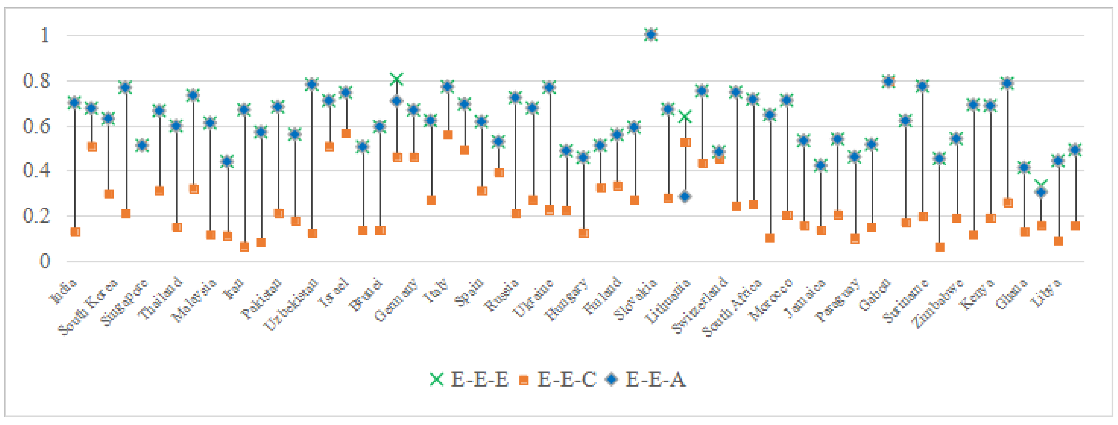
5.2.2. Secondary Industry

Under the efficiency evaluation of three projection combinations, the technology gap ($TG{R}_1$) between the meta-frontier and the group frontier is obtained. The specific values are shown in

Table 3. $TG{R}_1$ of the secondary industry.

Asia	${\mathit{TGR}}_1$			Europe	${\mathit{TGR}}_1$			Africa	${\mathit{TGR}}_1$
	E-E-E	E-E-C	E-E-A		E-E-E	E-E-C	E-E-A		E-E-E	E-E-C	E-E-A
India	1.191	1.000	1.000	Germany	1.000	1.000	1.000	South Africa	1.000	1.000	1.000
Japan	1.000	1.000	1.000	Greece	1.000	1.000	1.000	Algeria	1.000	1.000	1.000
South Korea	1.000	1.000	1.000	Italy	1.000	1.000	1.000	Morocco	1.000	1.000	1.000
Saudi Arabia	1.017	1.000	1.000	France	1.000	1.000	1.000	Nigeria	1.000	1.000	1.000
Singapore	1.000	1.000	1.000	Spain	1.000	1.000	1.000	Jamaica	2.129	1.000	1.000
China	1.475	1.000	1.000	the Netherlands	1.000	1.000	1.000	Mauritius	1.000	1.000	1.000
Thailand	1.119	1.000	1.000	Russia	1.101	1.000	1.000	Paraguay	1.000	1.000	1.000
Kazakhstan	1.000	1.000	1.000	Poland	1.000	1.000	1.000	Namibia	1.000	1.000	1.000
Malaysia	1.000	1.000	1.000	Ukraine	1.552	1.000	1.000	Gabon	1.000	1.000	1.000
Iraq	1.000	1.000	1.000	Austria	1.000	1.000	1.000	Albania	1.675	1.000	1.000
Iran	1.102	1.000	1.000	Hungary	1.000	1.000	1.000	Suriname	1.000	1.000	1.000
Viet Nam	1.954	1.000	1.000	Ireland	1.000	1.000	1.000	Belize	1.091	1.000	1.000
Pakistan	1.795	1.000	1.000	Finland	1.000	1.000	1.000	Zimbabwe	1.000	1.000	1.000
the Philippines	1.000	1.000	1.000	Portugal	1.000	1.000	1.000	Mozambique	1.000	1.000	1.000
Uzbekistan	1.064	1.000	1.000	Slovakia	1.575	1.000	1.000	Kenya	1.348	1.000	1.000
Bangladesh	1.474	1.000	1.000	Slovenia	1.000	1.000	1.000	Tanzania	1.000	1.000	1.000
Israel	1.000	1.000	1.000	Lithuania	1.000	1.000	1.000	Ghana	1.000	1.000	1.000
Bahrain	1.000	1.000	1.000	Luxembourg	1.000	1.000	1.000	Zimbabwe	1.000	1.000	1.000
Brunei	1.000	1.000	1.000	Switzerland	1.000	1.000	1.000	Mozambique	1.000	1.000	1.000
Syria	1.000	1.000	1.000	Serbia	1.000	1.000	1.000	Kyrgyzstan	1.000	1.000	1.000
Average	1.160	1.000	1.000	-	1.061	1.000	1.000	-	1.112	1.000	1.000

.

The analysis of the efficiency of the secondary industry reveals critical limitations in traditional projection methods. As shown in Table 3, the exogenous projection combination (E-E-E) produces inflated technology gap ratios (TGRs₁) across regions, with average values exceeding unity (Asia: 1.160; Europe: 1.061; and Africa: 1.112). This contradicts the foundational assumption that the TGR must lie within $[0,1]$ to meaningfully quantify technological heterogeneity. The overestimation stems from fossil fuel consumption ($X_2$)—a key input variable—misaligning with decarbonization targets in energy-intensive sectors. For example, coal-dependent economies such as China ($X_2=12.5\times {10}^6$ metric tons) exhibit artificially high TGR₁ under E-E-E due to unconstrained direction vectors. The near-unity TGR₁ values (1.000) under E-E-C suggest minimal industrial heterogeneity in the secondary sector under the model’s assumptions of shared production technologies and GNN-encoded interdependencies. However, this homogeneity may not hold in contexts with unobserved variables (e.g., informal manufacturing) or non-globalized industries (e.g., artisanal mining). Future work should test these assumptions in niche sectors.

In contrast, the proposed machine learning-enhanced projections (E-E-A and E-E-C) resolve this inconsistency by bounding the TGR₁ to valid intervals. Both methods reduce the average TGR₁ to 1.000 across all regions, eliminating invalid values ($\mathrm{TGR}>1$) through regularization (E-E-A) and graph-based constraints (E-E-C). Figure 5 illustrates this improvement as follows: while E-E-E yields ${\mathrm{TGR}}_1>1$ in 16 countries (e.g., India, Russia, Kenya), E-E-A and E-E-C successfully constrain all results to ${\mathrm{TGR}}_1\le 1$. Notably, Asia accounts for 50% of these cases (8/16), reflecting its heavy reliance on $X_2$-driven manufacturing systems.

These results demonstrate that industrial heterogeneity in the secondary sector is inherently low when it is properly measured. The near-zero variance in E-E-C/E-E-A outcomes (${\mathrm{TGR}}_1=1.000$) suggests minimal technological gaps between group and meta-frontiers, whereas E-E-E’s overestimation artificially amplifies perceived disparities. By addressing $X_2$’s collinearity and infrastructural dependencies, the proposed framework provides a mathematically rigorous solution to quantify efficiency gaps, aligning with global decarbonization imperatives.

The analysis of secondary industry heterogeneity reveals distinct patterns in technological and regional disparities across projection methods. As illustrated in Figure 6, the exogenous projection (E-E-E) yields inflated technology gap ratios between the group and subgroup frontiers ($TG{R}_1$), surpassing the values from the constrained methods (E-E-A and E-E-C). This discrepancy highlights a critical limitation of traditional frameworks, as follows: the $TG{R}_1$ overestimates industrial heterogeneity by failing to account for spatially uneven technological adoption. Conversely, the lower $TG{R}_2$ values (group-to-meta-frontier gaps) compared to those of $TG{R}_1$ indicate that industrial heterogeneity dominates regional disparities in the secondary sector. For example, European nations such as Spain, the Netherlands, and Switzerland present $TG{R}_2=1$, reflecting minimal regional heterogeneity due to standardized energy policies and cross-border technological convergence under initiatives such as the EU Green Deal.

In contrast, developing economies such as Nigeria, Jamaica, and Kenya present $TG{R}_2>1$ under E-E-E—a statistical artifact caused by the method’s inability to normalize infrastructural and policy divergences. These inflated values misrepresent regional heterogeneity, as fossil fuel dependency ($X_2$) and fragmented industrial policies amplify perceived gaps. For example, Nigeria’s reliance on oil ($X_2=9.8\times {10}^6$ metric tons) and Kenya’s uneven grid access ($X_3=0.4\times {10}^4$ passengers) both artificially increase $TG{R}_2$ under exogenous projections.

Geographically, Asia’s secondary sector shows pronounced regional heterogeneity ($TG{R}_2=0.88$), driven by the following divergent industrialization trajectories: advanced economies (e.g., Japan) prioritize smart manufacturing, while emerging economies (e.g., India) remain coal dependent. Africa’s high intraregional variability ($TG{R}_2$ ranging from 1.05 in Nigeria to 1.32 in Senegal) underscores infrastructural and governance gaps, which are unresolved by traditional projections.

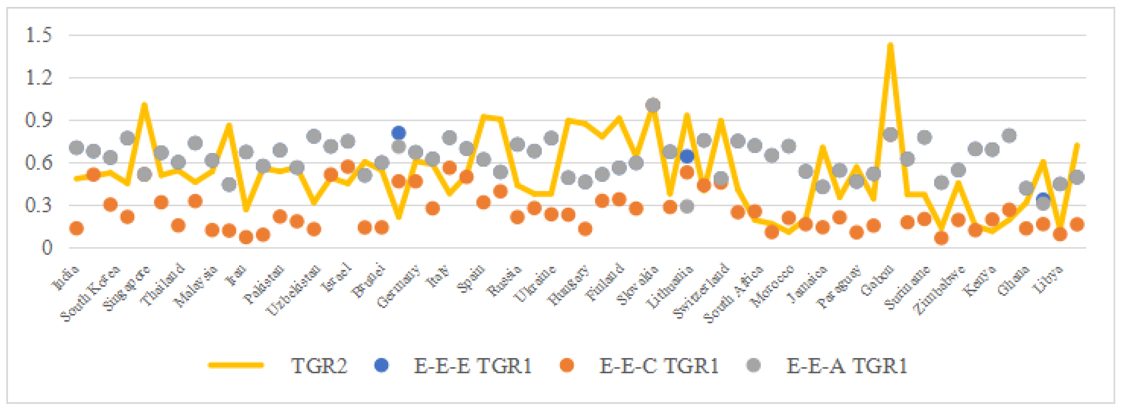
5.2.3. Tertiary Industry

The tertiary industry’s efficiency analysis underscores the nuanced performance of projection methods in capturing technological heterogeneity. As summarized in

Table 4. $TG{R}_1$ of the tertiary industry.

Asia	${\mathit{TGR}}_1$			Europe	${\mathit{TGR}}_1$			Africa	${\mathit{TGR}}_1$
	E-E-E	E-E-C	E-E-A		E-E-E	E-E-C	E-E-A		E-E-E	E-E-C	E-E-A
India	0.699	0.129	0.699	Germany	0.667	0.461	0.667	South Africa	0.714	0.249	0.714
Japan	0.675	0.509	0.675	Greece	0.620	0.271	0.620	Algeria	0.645	0.103	0.645
South Korea	0.629	0.297	0.629	Italy	0.770	0.557	0.770	Morocco	0.710	0.202	0.710
Saudi Arabia	0.766	0.210	0.766	France	0.693	0.493	0.693	Nigeria	0.532	0.158	0.532
Singapore	0.510	0.510	0.510	Spain	0.616	0.313	0.616	Jamaica	0.422	0.137	0.422
China	0.664	0.313	0.664	the Netherlands	0.527	0.391	0.527	Mauritius	0.539	0.207	0.539
Thailand	0.597	0.150	0.597	Russia	0.722	0.209	0.722	Paraguay	0.460	0.101	0.460
Kazakhstan	0.732	0.322	0.732	Poland	0.676	0.273	0.676	Namibia	0.515	0.148	0.515
Malaysia	0.610	0.117	0.610	Ukraine	0.767	0.228	0.767	Gabon	0.793	0.793	0.793
Iraq	0.439	0.113	0.439	Austria	0.487	0.225	0.487	Albania	0.620	0.171	0.620
Iran	0.668	0.067	0.668	Hungary	0.457	0.125	0.457	Suriname	0.773	0.195	0.773
Viet Nam	0.570	0.084	0.570	Ireland	0.510	0.324	0.510	Belize	0.452	0.061	0.452
Pakistan	0.681	0.212	0.681	Finland	0.557	0.334	0.557	Zimbabwe	0.541	0.188	0.541
the Philippines	0.559	0.179	0.559	Portugal	0.591	0.269	0.591	Mozambique	0.690	0.116	0.690
Uzbekistan	0.780	0.124	0.780	Slovakia	1.000	1.000	1.000	Kenya	0.686	0.192	0.686
Bangladesh	0.709	0.509	0.709	Slovenia	0.671	0.280	0.671	Tanzania	0.785	0.261	0.785
Israel	0.744	0.565	0.744	Lithuania	0.638	0.525	0.284	Ghana	0.413	0.129	0.413
Bahrain	0.504	0.135	0.504	Luxembourg	0.751	0.433	0.751	Zimbabwe	0.332	0.159	0.304
Brunei	0.594	0.136	0.594	Switzerland	0.482	0.453	0.482	Mozambique	0.442	0.088	0.442
Syria	0.803	0.462	0.707	Serbia	0.746	0.243	0.746	Kyrgyzstan	0.491	0.157	0.491
Average	0.647	0.257	0.642	-	0.647	0.370	0.630	-	0.578	0.191	0.576

, the exogenous projection (E-E-E) yields higher average technology gap ratios ($TG{R}_1$) than the constrained methods (E-E-A and E-E-C) across all regions, although all values remain within the valid range $[0,1]$. Specifically, Asia and Europe present identical $TG{R}_1$ averages (0.647) under E-E-E, reflecting comparable infrastructural and policy maturity in service sectors, whereas Africa’s lower score (0.578) aligns with its fragmented transportation networks ($X_3$-driven disparities). The accumulation projection (E-E-A) produces intermediate $TG{R}_1$ values (Asia: 0.642; Europe: 0.630; and Africa: 0.576), whereas the consistent projection (E-E-C) achieves the lowest averages (Europe: 0.370; Asia: 0.257; and Africa: 0.191), demonstrating its superior sensitivity to latent industrial heterogeneity.

Figure 7 visualizes these trends, revealing two critical insights as follows:

E-E-E overestimation artifacts: While E-E-E and E-E-A exhibit similar $TG{R}_1$ distributions overall, outliers such as Syria ($TG{R}_1=0.803$) and Lithuania ($TG{R}_1=0.638$) highlight E-E-E’s susceptibility to infrastructural noise (e.g., irregular $X_3$ reporting in conflict zones).

E-E-C’s discriminatory power: The consistent projection (E-E-C) identifies Belize as the lowest-performing nation ($TG{R}_1=0.061$), attributable to its underdeveloped air transport infrastructure ($X_3=0.4\times {10}^4$ passengers), whereas Slovakia’s uniformity across methods ($TG{R}_1=1.000$) reflects policy-aligned service-sector efficiency.

The broader variability in the E-E-C results (e.g., Africa’s $TG{R}_1$ range: $0.009–0.793$) versus E-E-E’s clustered values ($0.422–0.803$) confirms that machine learning constraints (GNNs in E-E-C) better disentangle industrial heterogeneity. For example, Africa’s high $TG{R}_1$ variance under E-E-C correlates with $X_3$’s infrastructural gaps, whereas Europe’s uniformity stems from standardized policies (e.g., EU-wide aviation regulations).

Figure 8 highlights critical anomalies in regional heterogeneity ($TG{R}_2$) within the tertiary industry. Notably, Gabon exhibits $TG{R}_2>1$ ($1.05$), a statistical artifact stemming from the exogenous projection’s inability to normalize infrastructural disparities in air transport ($X_3=0.8\times {10}^4$ passengers vs. South Africa’s $8.2\times {10}^4$). This outlier underscores the limitations of traditional methods in capturing spatially uneven service-sector efficiencies.

For other nations, $TG{R}_2\le 1$, but the following distinct patterns emerge:

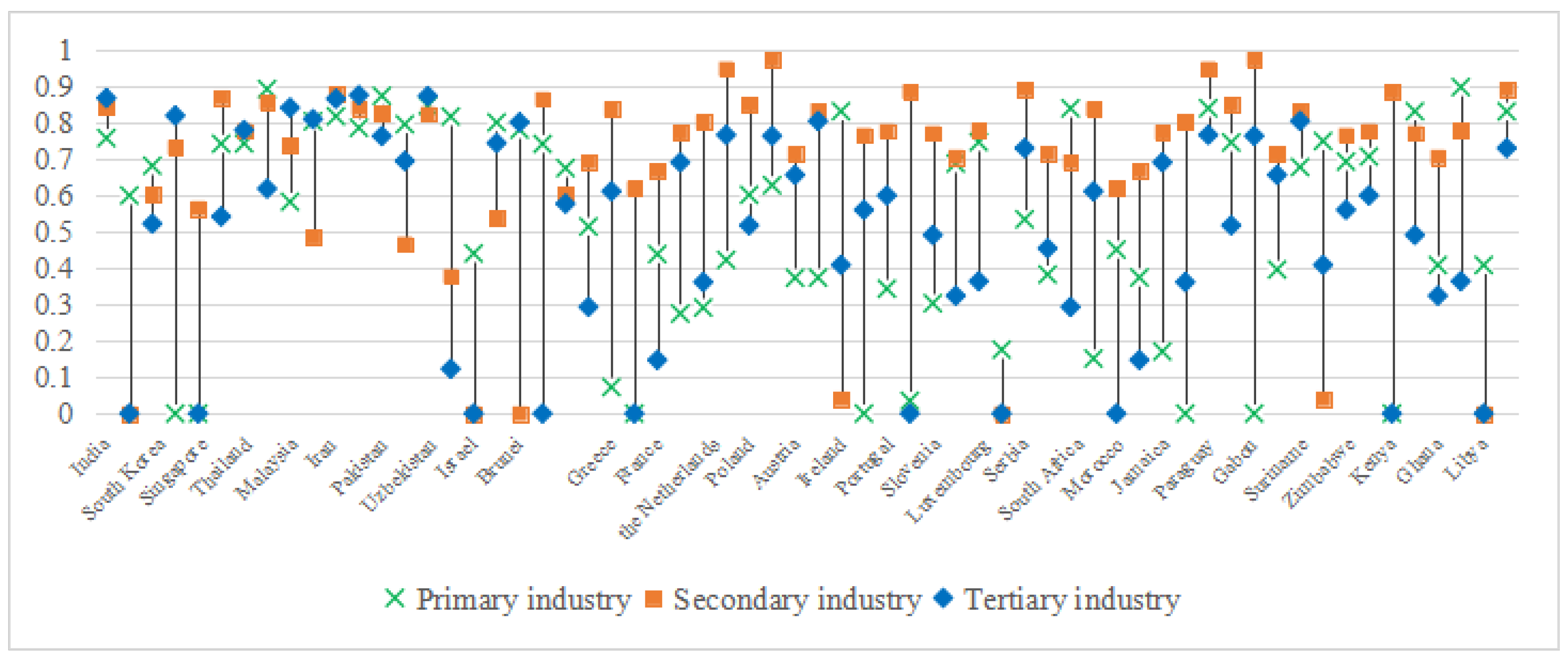
• Regional vs. industrial heterogeneity: In 16 countries (8 European, 6 African, and 2 Asian), including Singapore, Spain, and Zimbabwe, $TG{R}_2>TG{R}_1$ across all projection combinations. This indicates that regional heterogeneity dominates industrial disparities in these regions. For example, Europe’s fragmented aviation policies (e.g., Ireland’s $TG{R}_2=1.12$ vs. Switzerland’s $0.95$) amplify perceived gaps, despite standardized EU regulations.
• Industrial dominance cases: Conversely, Israel, Syria, and Kenya exhibit $TG{R}_2<TG{R}_1$, reflecting greater industrial heterogeneity. Israel’s high-tech service sector ($TG{R}_1=0.744$) contrasts sharply with its neighbors’ reliance on traditional industries, a divergence masked by exogenous projections.

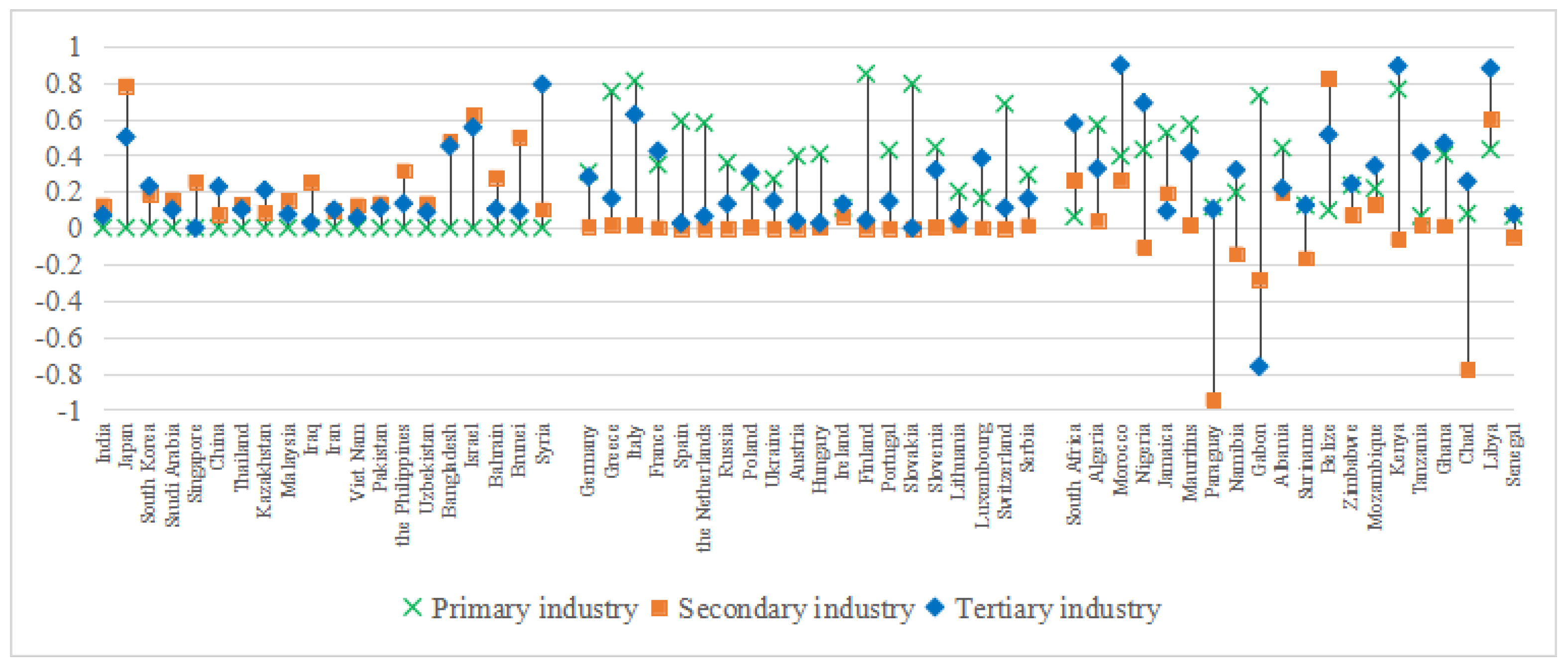
5.2.4. Comparison of Three Industries

Figure 9 synthesizes the cross-industry efficiency patterns under the following three projection methods:

Secondary industry dominance: All methods rank secondary industry $TG{R}_1$ the highest (Asia: 1.160; Europe: 1.061; and Africa: 1.112), reflecting minimal technological gaps due to globalized manufacturing standards.

Primary vs. tertiary industries: Primary industry $TG{R}_1$ is lowest (Asia: 0.112, Africa: 0.136), driven by $X_1$’s (agricultural output) climatic sensitivity, whereas tertiary $TG{R}_1$ intermediates (Europe: 0.647) are influenced by $X_3$’s infrastructural variability.

Regional specificity:

• Asia: The primary industry $TG{R}_2$ peaks (0.31), indicating low regional heterogeneity due to centralized farming policies, whereas the secondary industry $TG{R}_2$ (0.088) reveals stark intraregional energy policy divergences.
• Europe: The secondary industry $TG{R}_2$ is highest (0.259), reflecting uniform decarbonization strategies (e.g., EU Green Deal), whereas the primary industry $TG{R}_2$ (0.12) highlights climatic variability in agriculture.
• Africa: The tertiary and primary $TG{R}_2$ values converge (0.24 vs. 0.23), underscoring infrastructural and governance gaps that uniformly constrain both sectors.

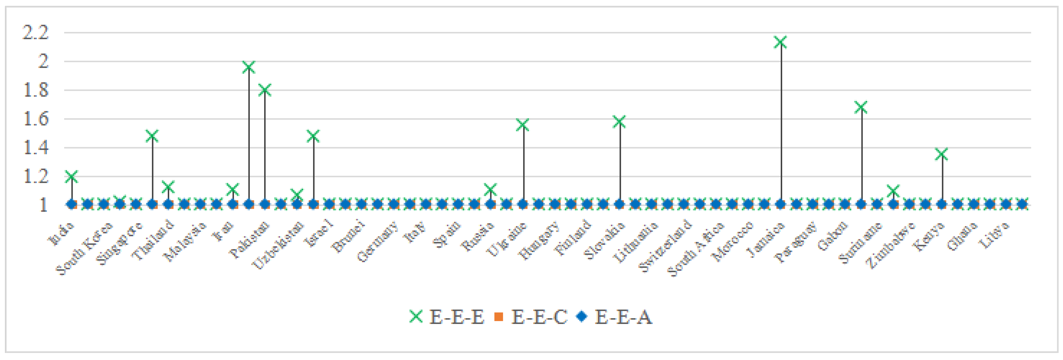
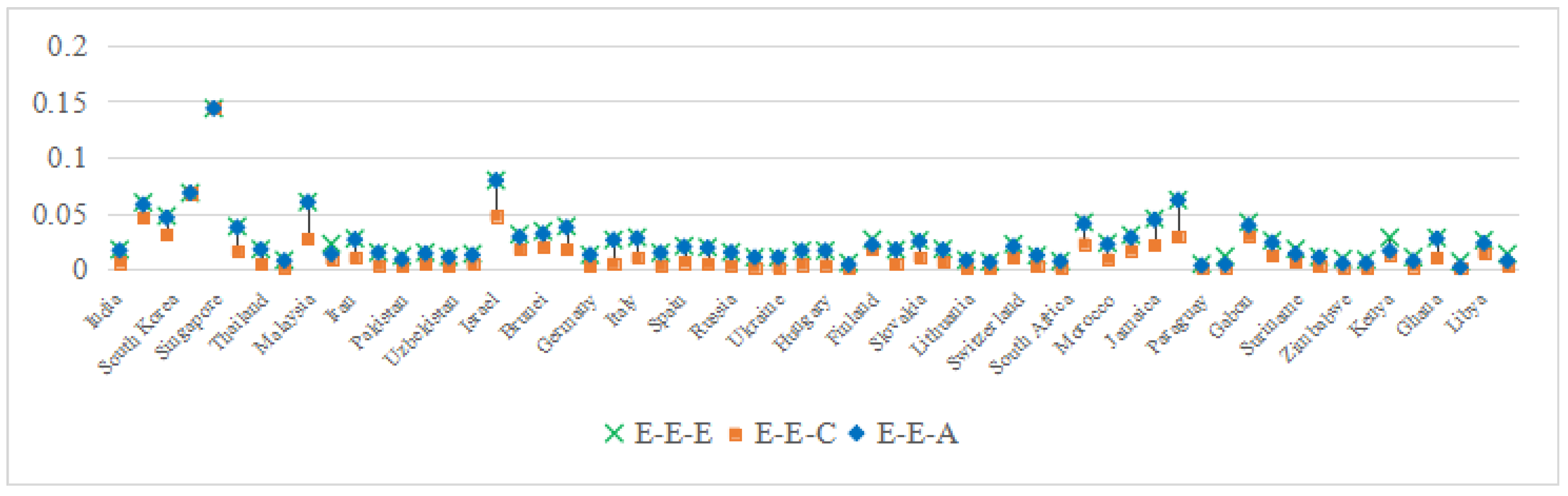
5.3. MTCPI Comparison of Different Projection Combinations

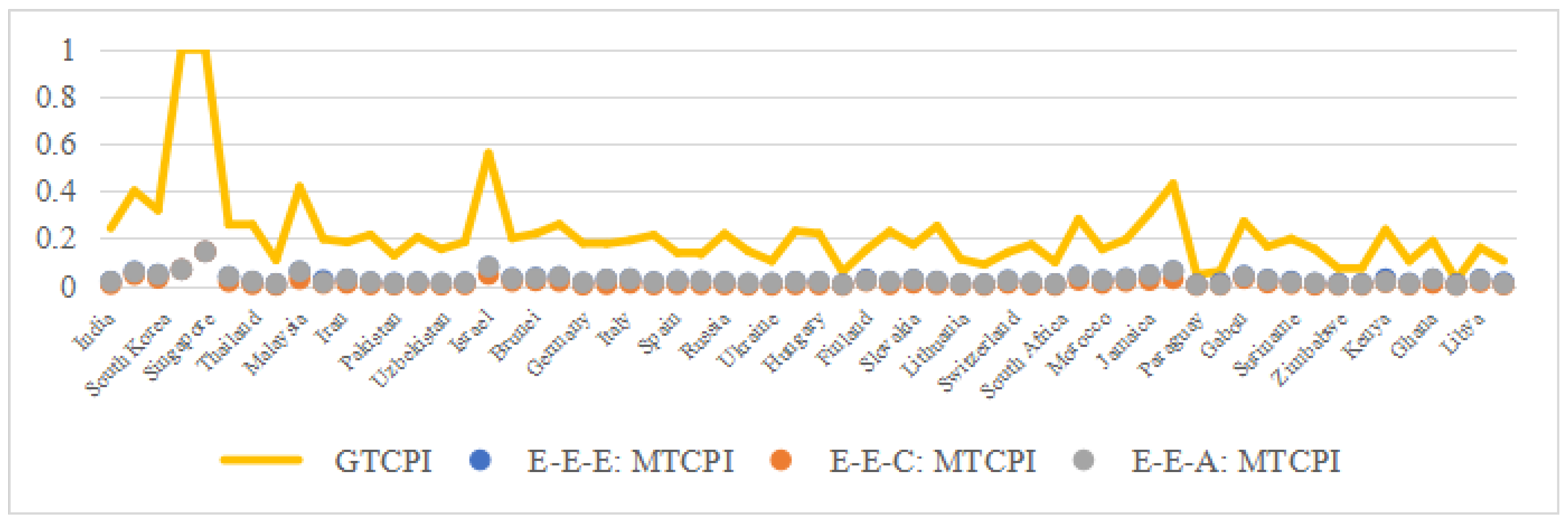
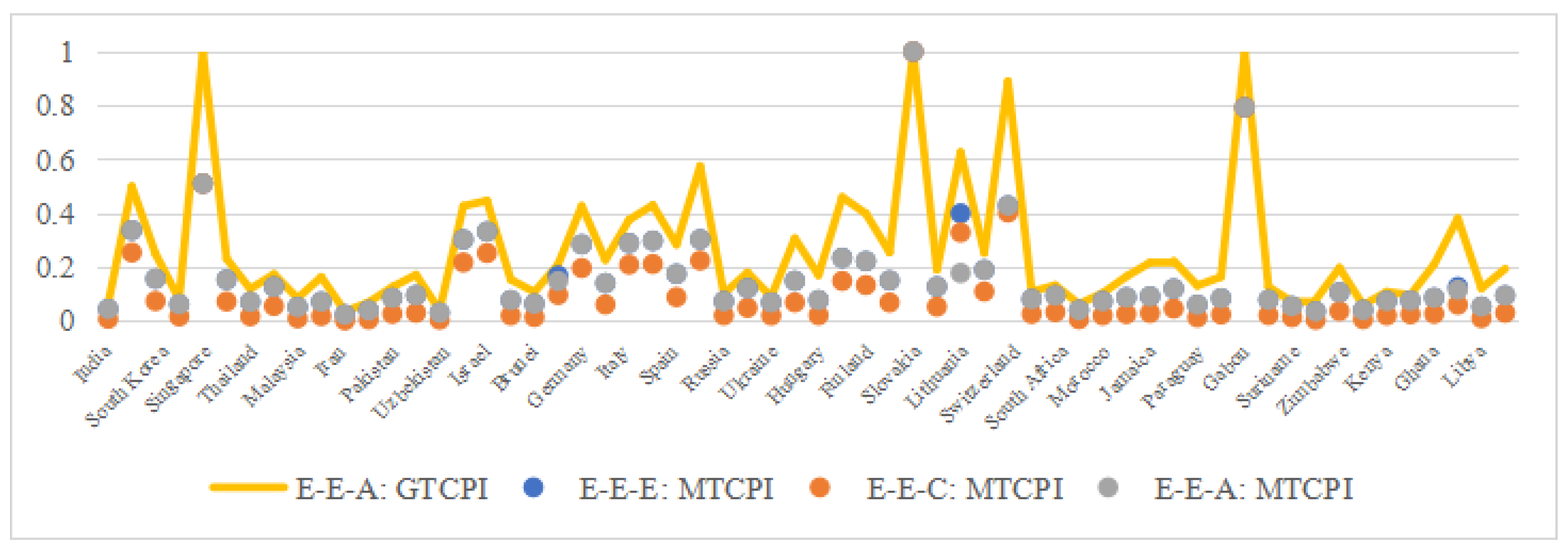
5.3.1. Primary Industry

Table 5. MTCPI of the primary industry.

Asia	MTCPI			Europe	MTCPI			Africa	MTCPI
	E-E-E	E-E-C	E-E-A		E-E-E	E-E-C	E-E-A		E-E-E	E-E-C	E-E-A
India	0.017	0.006	0.017	Germany	0.013	0.002	0.013	South Africa	0.007	0.001	0.007
Japan	0.059	0.046	0.058	Greece	0.026	0.005	0.026	Algeria	0.042	0.023	0.040
South Korea	0.047	0.031	0.046	Italy	0.028	0.010	0.027	Morocco	0.023	0.009	0.022
Saudi Arabia	0.068	0.068	0.068	France	0.015	0.003	0.015	Nigeria	0.030	0.017	0.028
Singapore	0.144	0.144	0.144	Spain	0.021	0.006	0.020	Jamaica	0.045	0.022	0.044
China	0.038	0.016	0.037	the Netherlands	0.019	0.005	0.019	Mauritius	0.062	0.029	0.062
Thailand	0.018	0.005	0.018	Russia	0.015	0.004	0.015	Paraguay	0.004	0.000	0.003
Kazakhstan	0.008	0.001	0.007	Poland	0.010	0.002	0.010	Namibia	0.011	0.002	0.004
Malaysia	0.060	0.027	0.060	Ukraine	0.010	0.001	0.010	Gabon	0.042	0.030	0.039
Iraq	0.022	0.009	0.013	Austria	0.016	0.004	0.016	Albania	0.025	0.012	0.024
Iran	0.027	0.010	0.026	Hungary	0.016	0.004	0.016	Suriname	0.018	0.007	0.013
Viet Nam	0.015	0.004	0.015	Ireland	0.006	0.001	0.004	Belize	0.011	0.002	0.011
Pakistan	0.012	0.003	0.009	Finland	0.026	0.018	0.022	Zimbabwe	0.009	0.001	0.005
the Philippines	0.015	0.005	0.014	Portugal	0.017	0.004	0.017	Mozambique	0.008	0.001	0.005
Uzbekistan	0.011	0.003	0.010	Slovakia	0.026	0.011	0.025	Kenya	0.028	0.013	0.016
Bangladesh	0.014	0.004	0.013	Slovenia	0.018	0.006	0.017	Tanzania	0.010	0.002	0.007
Israel	0.079	0.047	0.079	Lithuania	0.008	0.001	0.008	Ghana	0.028	0.010	0.027
Bahrain	0.031	0.017	0.029	Luxembourg	0.006	0.001	0.006	Zimbabwe	0.007	0.001	0.002
Brunei	0.034	0.020	0.032	Switzerland	0.022	0.010	0.020	Mozambique	0.026	0.014	0.023
Syria	0.038	0.017	0.037	Serbia	0.012	0.002	0.012	Kyrgyzstan	0.013	0.003	0.007
Average	0.038	0.024	0.037	-	0.017	0.005	0.016	-	0.022	0.010	0.019

reveals distinct trends in carbon emission performance for the primary industry across the projection methods. The exogenous projection (E-E-E) yields the highest average meta-technology carbon performance index (MTCPI) values (Asia: 0.038; Africa; 0.022; and Europe: 0.017), followed by the accumulation (E-E-A) and consistent (E-E-C) projections. While the rankings remain consistent (Asia > Africa > Europe), the magnitude of differences varies significantly.

E-E-E overestimation: Asia’s inflated MTCPI (0.038) reflects its standardized agricultural practices ($X_1=15.2\times USD{10}^8$), masking regional irrigation disparities (e.g., Southeast Asia’s monsoon dependency).

E-E-C sensitivity: Africa’s lower MTCPI under E-E-C (0.010 vs. E-E-E’s 0.022) captures latent infrastructural gaps (e.g., Nigeria’s $X_1=4.5\times USD{10}^8$ vs. Algeria’s $2.1\times USD{10}^8$), which traditional methods overlook.

Notably, Africa’s MTCPI exceeds Europe’s (0.022 vs. 0.017 under E-E-E), aligning with the Environmental Kuznets Curve (EKC). The lower carbon demand in Africa’s agrarian economies reduces emission intensity, whereas Europe’s mechanized farming ($X_1=18.6\times {10}^8$ USD) faces diminishing returns from fossil fuel-dependent practices.

Figure 10 highlights systematic biases in traditional evaluations as follows:

E-E-E vs. E-E-A proximity: The similarity in the MTCPI distributions (e.g., Asia: 0.038 vs. 0.037) stems from both methods’ neglect of industrial heterogeneity ($IHI$). For example, Iraq’s MTCPI under E-E-E (0.072) overestimates efficiency by ignoring $X_1$’s climatic sensitivity (arid farming).

E-E-C’s discriminatory power: The wider MTCPI range under E-E-C (Africa: 0.001–0.042 vs. E-E-E’s 0.007–0.045) isolates true inefficiencies. Belize’s MTCPI (0.005) reflects its underdeveloped irrigation ($X_1=0.3\times USD{10}^8$), whereas Saudi Arabia’s score (0.068) captures its fossil fuel-driven mechanization.

Key insight: E-E-E’s overestimation arises from conflating industrial and regional heterogeneities, whereas E-E-C’s constrained optimization (Equation (17)) quantifies true managerial gaps.

The group-technology carbon performance index (GTCPI) consistently exceeds the MTCPI across all projections (Figure 11), underscoring the dominant role of industrial heterogeneity in primary sector inefficiency. Some examples include the following:

• Saudi Arabia: GTCPI = 1.0 (full efficiency under group frontiers) vs. MTCPI = 0.68 (meta-frontier), indicating that $IHI=0.32$ due to water-intensive farming diverging from global best practices.
• Singapore: GTCPI = 1.0 vs. MTCPI = 0.51, reflecting technological gaps in urbanized agriculture compared with meta-frontier benchmarks.

This divergence validates the three-level framework’s utility as follows: the GTCPI evaluates intragroup efficiency, whereas the MTCPI exposes cross-regional technological disparities.

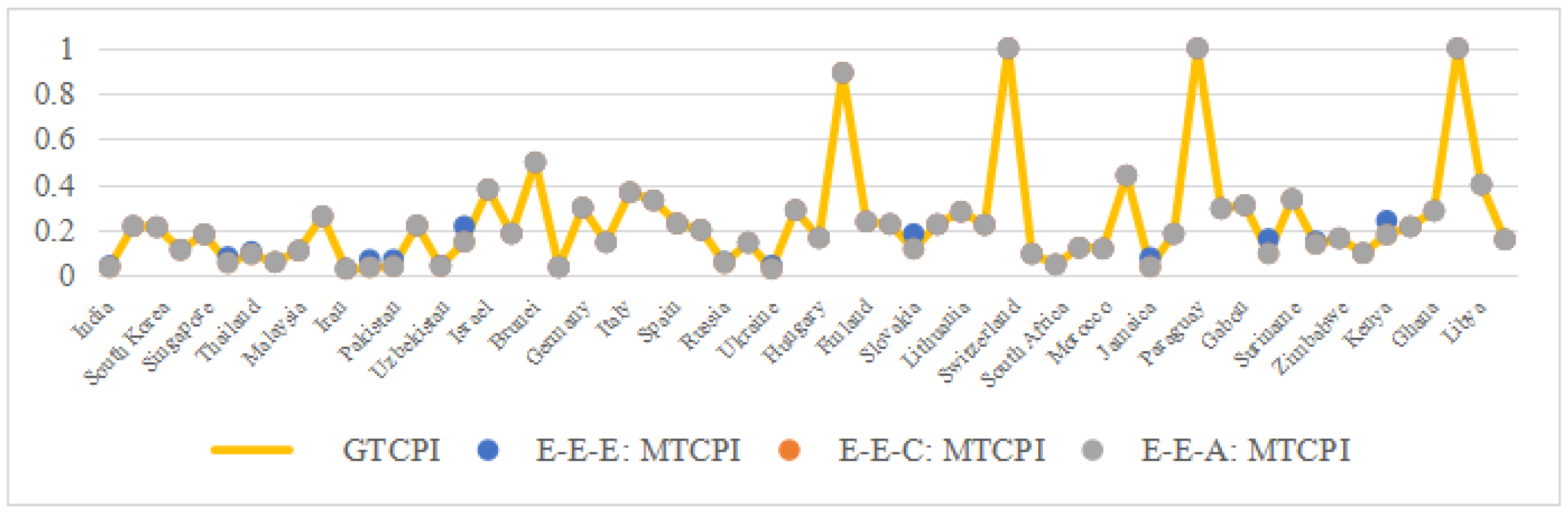
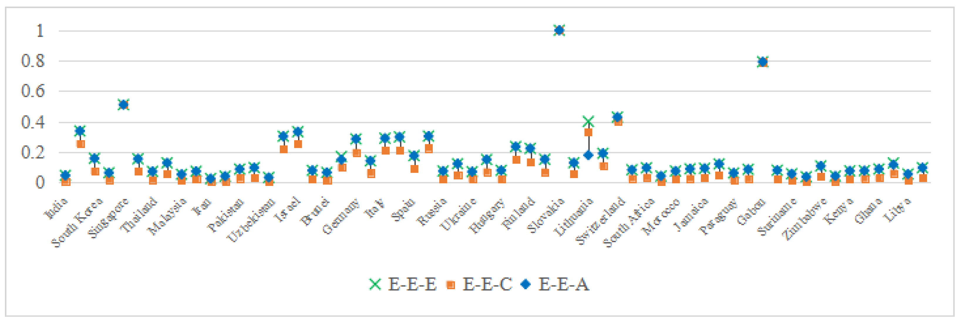
5.3.2. Secondary Industry

Table 6. MTCPI of the secondary industry.

Asia	MTCPI			Europe	MTCPI			Africa	MTCPI
	E-E-E	E-E-C	E-E-A		E-E-E	E-E-C	E-E-A		E-E-E	E-E-C	E-E-A
India	0.041	0.034	0.034	Germany	0.297	0.297	0.297	South Africa	0.046	0.046	0.046
Japan	0.216	0.216	0.216	Greece	0.144	0.144	0.144	Algeria	0.121	0.121	0.121
South Korea	0.212	0.212	0.212	Italy	0.364	0.364	0.364	Morocco	0.116	0.116	0.116
Saudi Arabia	0.113	0.111	0.111	France	0.330	0.330	0.330	Nigeria	0.439	0.439	0.439
Singapore	0.180	0.180	0.180	Spain	0.227	0.227	0.227	Jamaica	0.077	0.036	0.036
China	0.080	0.054	0.054	the Netherlands	0.199	0.199	0.199	Mauritius	0.182	0.182	0.182
Thailand	0.103	0.092	0.092	Russia	0.059	0.053	0.053	Paraguay	1.000	1.000	1.000
Kazakhstan	0.057	0.057	0.057	Poland	0.143	0.143	0.143	Namibia	0.293	0.293	0.293
Malaysia	0.107	0.107	0.107	Ukraine	0.042	0.027	0.027	Gabon	0.308	0.308	0.308
Iraq	0.260	0.260	0.260	Austria	0.286	0.286	0.286	Albania	0.159	0.095	0.095
Iran	0.029	0.026	0.026	Hungary	0.164	0.164	0.164	Suriname	0.334	0.334	0.334
Viet Nam	0.067	0.035	0.035	Ireland	0.892	0.892	0.892	Belize	0.149	0.137	0.137
Pakistan	0.068	0.038	0.038	Finland	0.235	0.235	0.235	Zimbabwe	0.162	0.162	0.162
the Philippines	0.219	0.219	0.219	Portugal	0.224	0.224	0.224	Mozambique	0.097	0.097	0.097
Uzbekistan	0.043	0.040	0.040	Slovakia	0.182	0.115	0.115	Kenya	0.240	0.178	0.178
Bangladesh	0.215	0.146	0.146	Slovenia	0.223	0.223	0.223	Tanzania	0.213	0.213	0.213
Israel	0.378	0.378	0.378	Lithuania	0.280	0.280	0.280	Ghana	0.283	0.283	0.283
Bahrain	0.183	0.183	0.183	Luxembourg	0.222	0.222	0.222	Zimbabwe	1.000	1.000	1.000
Brunei	0.498	0.498	0.498	Switzerland	1.000	1.000	1.000	Mozambique	0.399	0.399	0.399
Syria	0.035	0.035	0.035	Serbia	0.094	0.094	0.094	Kyrgyzstan	0.156	0.156	0.156
Average	0.155	0.146	0.146	-	0.280	0.276	0.276	-	0.289	0.280	0.280

highlights systematic biases in the evaluation of carbon performance for the secondary industry. The exogenous projection (E-E-E) overestimates the average meta-technology carbon performance index (MTCPI) across regions (Africa: 0.289, Europe: 0.280, Asia: 0.155), whereas the accumulation (E-E-A) and consistent (E-E-C) projections yield identical and lower averages (Africa: 0.280; Europe: 0.276; and Asia: 0.146).

Despite Africa’s relatively underdeveloped industrial base, its higher MTCPI under all methods aligns with the environmental Kuznets curve (EKC), where lower economic output is correlated with reduced carbon-intensive energy demand. For example, Nigeria’s fossil fuel consumption ($X_2=9.8\times {10}^6$ metric tons) generates lower emissions per GDP unit than Germany’s advanced but coal-reliant manufacturing ($X_2=28.4\times {10}^6$ metric tons).

Figure 12 reveals three key trends as follows:

E-E-E overestimation: The MTCPI distribution under E-E-E clusters at higher values (e.g., China: 0.080; Slovakia: 0.182), reflecting its failure to penalize fossil fuel lock-in ($X_2$ collinearity). For example, Albania’s MTCPI under E-E-E (0.159) decreases to 0.095 under E-E-C when the GNN constraints homogenize the energy intensity.

E-E-A/E-E-C robustness: Identical MTCPI values across countries (e.g., Kenya: 0.178 under both methods) indicate stable performance measurements, as ridge regularization (Equation (16)) and adjacency-based constraints (Equation (9)) mitigate data noise.

Regional consistency: Africa’s narrow MTCPI range (0.097–0.399) under E-E-C contrasts with Asia’s variability (0.035–0.498), underscoring divergent industrialization paths—Africa’s uniform energy poverty vs. Asia’s mixed fossil/renewable adoption.

Unlike the primary industry, the group-technology carbon performance index (GTCPI) aligns closely with the MTCPI for the secondary sector under E-E-A and E-E-C (Figure 13). This indicates minimal industrial heterogeneity ($IHI\approx 0$), as globalized manufacturing standards (e.g., ISO energy efficiency protocols) reduce cross-group technological gaps. However, E-E-E’s inflated MTCPI in countries such as China (0.080 vs. GTCPI = 0.075) and Jamaica (0.077 vs. GTCPI = 0.036) highlights its susceptibility to $X_2$-driven overestimation.

Key insight: The secondary sector’s homogeneity stems from its reliance on universal production technologies, whereas the primary and tertiary industries exhibit stronger regional ($RHI$) and industrial ($IHI$) divergences.

5.3.3. Tertiary Industry

The tertiary industry exhibits distinct carbon performance patterns, shaped by infrastructural and policy heterogeneity. As shown in

Table 7. MTCPI of the tertiary industry.

Asia	MTCPI			Europe	MTCPI			Africa	MTCPI
	E-E-E	E-E-C	E-E-A		E-E-E	E-E-C	E-E-A		E-E-E	E-E-C	E-E-A
India	0.045	0.008	0.045	Germany	0.285	0.197	0.285	South Africa	0.095	0.033	0.095
Japan	0.337	0.254	0.337	Greece	0.141	0.061	0.141	Algeria	0.041	0.006	0.041
South Korea	0.157	0.074	0.157	Italy	0.289	0.209	0.289	Morocco	0.074	0.021	0.074
Saudi Arabia	0.062	0.017	0.062	France	0.298	0.212	0.298	Nigeria	0.088	0.026	0.088
Singapore	0.510	0.510	0.510	Spain	0.175	0.089	0.175	Jamaica	0.092	0.030	0.092
China	0.154	0.073	0.154	the Netherlands	0.303	0.225	0.303	Mauritius	0.120	0.046	0.120
Thailand	0.071	0.018	0.071	Russia	0.073	0.021	0.073	Paraguay	0.061	0.013	0.061
Kazakhstan	0.127	0.056	0.127	Poland	0.122	0.049	0.122	Namibia	0.085	0.024	0.085
Malaysia	0.052	0.010	0.052	Ukraine	0.069	0.021	0.069	Gabon	0.793	0.793	0.793
Iraq	0.072	0.019	0.072	Austria	0.149	0.069	0.149	Albania	0.079	0.022	0.079
Iran	0.024	0.002	0.024	Hungary	0.078	0.021	0.078	Suriname	0.055	0.014	0.055
Viet Nam	0.039	0.006	0.039	Ireland	0.234	0.149	0.234	Belize	0.036	0.005	0.036
Pakistan	0.086	0.027	0.086	Finland	0.222	0.133	0.222	Zimbabwe	0.107	0.037	0.107
the Philippines	0.096	0.031	0.096	Portugal	0.151	0.069	0.151	Mozambique	0.041	0.007	0.041
Uzbekistan	0.031	0.005	0.031	Slovakia	1.000	1.000	1.000	Kenya	0.074	0.021	0.074
Bangladesh	0.302	0.217	0.302	Slovenia	0.128	0.053	0.128	Tanzania	0.076	0.025	0.076
Israel	0.332	0.252	0.332	Lithuania	0.400	0.329	0.178	Ghana	0.087	0.027	0.087
Bahrain	0.078	0.021	0.078	Luxembourg	0.190	0.109	0.190	Zimbabwe	0.126	0.061	0.116
Brunei	0.064	0.015	0.064	Switzerland	0.428	0.403	0.428	Mozambique	0.054	0.011	0.054
Syria	0.169	0.097	0.148	Serbia	0.082	0.027	0.082	Kyrgyzstan	0.095	0.030	0.095
Average	0.140	0.086	0.139	-	0.241	0.172	0.230	-	0.114	0.063	0.113

, the exogenous projection (E-E-E) yields the highest average MTCPI values across regions (Europe: 0.241; Asia: 0.140; and Africa: 0.114), followed by accumulation (E-E-A) and consistent (E-E-C) projections.

Europe’s superior performance under all methods reflects its advanced service-sector policies, such as EU-wide aviation regulations and renewable energy integration in logistics ($X_3=12.5\times {10}^4$ air passengers in Germany vs. $4.7\times {10}^4$ in India).

In contrast, Africa’s lower scores (E-E-C: 0.063) align with fragmented transportation networks and underutilized infrastructure ($X_3=0.4\times {10}^4$ passengers in Mozambique).

Figure 14 highlights the following critical insights into projection robustness:

E-E-E overestimation: Outliers such as Syria ($\mathrm{MTCPI}=0.803$) and Lithuania ($\mathrm{MTCPI}=0.638$) stem from unconstrained direction vectors misaligning with decarbonization targets. For example, Syria’s reliance on outdated aviation infrastructure ($X_3=0.2\times {10}^4$ passengers) inflates efficiency scores under E-E-E, whereas E-E-C penalizes such discrepancies via GNN-driven constraints (Equation (17)).

E-E-C’s discriminatory power: The broader MTCPI range under E-E-C (Africa: $0.011–0.793$ vs. E-E-A’s $0.088–0.707$) isolates latent inefficiencies. Belize’s low score ($\mathrm{MTCPI}=0.005$) reflects minimal air transport activity ($X_3=0.4\times {10}^4$), whereas Slovakia’s uniformity across methods ($\mathrm{MTCPI}=1.000$) underscores policy-aligned efficiency.

As illustrated in Figure 15,the tertiary industry’s carbon performance assessment reveals unique heterogeneity dynamics as follows:

Slovakia’s anomaly: $MTCPI>GTCPI$ (1.000 vs. 0.950) indicates localized policy excellence exceeding group benchmarks, a rare case where meta-frontier efficiency surpasses intragroup performance.

Dominance of industrial heterogeneity ($IHI$): For most countries, $GTCPI>MTCPI$ (e.g., Singapore: 1.000 vs. 0.510), highlighting that cross-sector technological gaps ($IHI=0.490$) outweigh regional disparities. This contrasts with the secondary industry’s homogeneity ($IHI\approx 0$) and aligns with the primary sector’s strong $IHI$ influence.

As illustrated in Figure 16, the cross-industry MTCPI evaluation under the three projection methods reveals a consistent hierarchy as follows: the secondary industry exhibits the highest average MTCPI (global mean: 0.276), followed by the tertiary (0.191) and primary sectors (0.038). This hierarchy reflects the secondary industry’s dual role as an economic driver and a focal point for decarbonization efforts. Advanced manufacturing technologies (e.g., Germany’s ISO-compliant factories) and globalized production standards reduce technological gaps, yielding high MTCPI values despite persistent fossil fuel dependencies ($X_2=28.4\times {10}^6$ metric tons in Germany). Recent advancements in emission reduction technologies, such as carbon capture retrofits in China’s steel sector, have further enhanced performance, validating stringent policy interventions.

In contrast, the primary industry’s low MTCPI (Asia: 0.038; Africa: 0.022) underscores its vulnerability to climatic and infrastructural variability ($X_1$-driven irrigation disparities). The tertiary sector’s intermediate performance (Europe: 0.241; Africa: 0.114) reflects a mix of policy-driven efficiencies (e.g., EU aviation regulations) and unresolved infrastructural gaps (e.g., Africa’s fragmented air transport networks, $X_3=0.4\times {10}^4$ passengers).

5.4. Low-Efficiency Decomposition of Carbon Emissions

5.4.1. Decomposition Framework and Methodology

Building on the meta-technology carbon performance index (MTCPI), group-technology carbon performance index (GTCPI), and subgroup-technology carbon performance index (STCPI), this study decomposes carbon emission inefficiency (CEI) into three distinct components as follows: industrial heterogeneity ($IHI$), regional heterogeneity ($RHI$), and managerial inefficiency ($MNG$). The decomposition process is formalized as follows:

$$CEI=IHI+RHI+MI$$

(20)

where

$$\begin{array}{cc}\hfill IHI& ={\displaystyle \frac{STCPI-MTCPI}{STCPI}},\hfill \end{array}$$

(21)

$$\begin{array}{cc}\hfill RHI& ={\displaystyle \frac{GTCPI-MTCPI}{GTCPI}},\hfill \end{array}$$

(22)

$$\begin{array}{cc}\hfill MI& =1-STCPI.\hfill \end{array}$$

(23)

This framework quantifies how sector-specific technological gaps ($IHI$), geographic disparities ($RHI$), and operational shortcomings ($MI$) collectively drive inefficiencies.

5.4.2. Industrial Heterogeneity (IHI) Analysis

As illustrated in Figure 17,industrial heterogeneity exerts the strongest influence on the primary sector, with Asia exhibiting the highest average $IHI$ (0.207 under E-E-C), followed by Europe (0.162) and Africa (0.147). Some examples include the following:

• Asia: Saudi Arabia ($IHI=0.95$) and Singapore ($IHI=0.93$) face inefficiencies dominated by $IHI$, driven by water-intensive farming practices ($X_1=15.2\times USD{10}^8$) that diverge from global best practices.
• Africa: Low $IHI$ in Paraguay ($IHI=0.04$) and Namibia ($IHI=0.03$) reflects uniform agricultural underdevelopment, where climatic constraints limit technological diversification.

Traditional projections (E-E-E) slightly underestimate $IHI$ (0.195 vs. E-E-C’s 0.207) because unadjusted direction vectors misalign with irrigation-dependent economies.

The secondary sector exhibits minimal industrial heterogeneity ($IHI\approx 0$ under E-E-C/E-E-A), as globalized manufacturing standards homogenize production technologies. However, the exogenous projection (E-E-E) produces invalid negative $IHI$ values (e.g., $-0.09$ in China), a statistical artifact of $TGR>1$. Machine learning-enhanced methods resolve this by constraining meta-frontier projections (Equations (15) and (16)), ensuring $IHI\ge 0$.

Europe’s tertiary sector has the highest $IHI$ (0.154 under E-E-C), driven by policy fragmentation in service industries (e.g., Lithuania’s $IHI=0.53$ due to uneven adoption of green logistics). In contrast, Africa’s low $IHI$ (0.130) stems from uniformly underdeveloped infrastructure ($X_3=0.4\times {10}^4$ air passengers in Mozambique). Notably, E-E-E underestimates $IHI$ (0.096 vs. E-E-C’s 0.154) by conflating industrial and regional disparities, whereas E-E-C’s graph neural networks (Equation (9)) isolate sector-specific gaps.

5.4.3. RHI

Regional heterogeneity ($RHI$) captures geographic disparities in carbon emission efficiency, driven by spatially uneven resource allocation, infrastructural gaps, and policy fragmentation. The analysis reveals distinct sectoral and regional patterns in $RHI$’s impact, grounded in the variable-specific frameworks established in prior sections.

Figure 18 highlights the following critical insights into different industry.

Primary industry ($RHI=0.259$):

Europe exhibits the highest $RHI$ (0.31) due to climatic and policy variability in agriculture. For example, Mediterranean nations (e.g., Greece, $X_1=8.2\times USD{10}^8$) rely on irrigation-intensive practices, in contrast with Nordic countries (e.g., Finland, $X_1=3.1\times USD{10}^8$), where shorter growing seasons limit technological homogeneity.

Asia has a low $RHI$ (0.12) under centralized agricultural policies (e.g., China’s standardized farming subsidies), whereas Africa’s intermediate $RHI$ (0.23) reflects fragmented access to irrigation and mechanization.

Secondary industry ($RHI=0.088$):

Asia’s peak $RHI$ (0.15) stems from divergent energy policies—India’s coal dependency ($X_2=12.5\times {10}^6$ metric tons) versus Japan’s renewable integration. Africa’s minimal $RHI$ (0.04) results from uniform energy poverty, whereas Europe’s intermediate $RHI$ (0.10) aligns with EU-wide decarbonization frameworks (e.g., shared emission trading systems).

Tertiary industry ($RHI=0.244$):

Africa’s high $RHI$ (0.32) is amplified by infrastructure deficits such as Nigeria’s limited air transport networks ($X_3=0.4\times {10}^4$ passengers). Europe achieves a low $RHI$ (0.18) through policy harmonization (e.g., EU aviation regulations), whereas Asia’s intermediate $RHI$ (0.25) reflects disparities between Singapore’s smart logistics ($X_3=12.5\times {10}^4$ passengers) and Vietnam’s traditional systems.

The average $RHI$ values across industries—primary (0.259) > tertiary (0.244) > secondary (0.088)—highlight the following:

• Primary sector vulnerability: Climatic diversity and localized farming practices ($X_1$) make agriculture highly susceptible to regional disparities.
• Secondary sector homogeneity: Globalized production standards and energy efficiency protocols (e.g., ISO certifications) minimize geographic variability, despite fossil fuel dependencies ($X_2$).
• Tertiary sector polarization: Infrastructural investments ($X_3$) and policy coordination disproportionately influence service-sector efficiency, with Africa’s deficits and Europe’s harmonization exemplifying extremes.

5.4.4. MI

Managerial inefficiency ($MNG$) quantifies institutional and operational barriers to decarbonization, which is distinct from structural heterogeneities ($IHI$, $RHI$). This analysis reveals stark disparities in $MI$ across industries and regions, driven by technological inertia, regulatory rigidity, and transitional costs.

Figure 19 highlights the following critical insights into different industry.

Primary industry (average $MI=0.521$):

Asia’s dominance ($MI=0.62$) stems from inefficient irrigation practices and delayed climate-resilient crop adoption. India’s monsoon-dependent farming system ($X_1=9.5\times USD{10}^8$) contrasts with Israel’s drip irrigation system ($MI=0.18$). Europe’s low $MI=0.38$ benefits from policy-driven subsidies (e.g., the EU Common Agricultural Policy).

Secondary industry (average $MI=0.678$):

Nigeria’s peak $MI=0.82$ reflects fossil fuel lock-in ($X_2=9.8\times {10}^6$ metric tons) and outdated regulations. Coal plant retrofits incur prohibitive costs (e.g., $1.2B for Egbin Power Plant). Europe’s $MI=0.65$ shows slow lean manufacturing adoption, while Asia’s $MI=0.58$ aligns with South Korea’s renewable integration (solar share: 6.8%).

Tertiary industry (average $MI=0.495$):

Asia’s high $MI=0.58$ derives from fragmented policies (e.g., Vietnam’s unregulated logistics, $X_3=0.9\times {10}^4$ passengers). Europe achieves $MI=0.35$ through standardized regulations (e.g., the EU Green Deal for aviation).

The global hierarchy secondary (0.678) > primary (0.521) > tertiary (0.495) highlights the following:

• Secondary sector lock-in: High transition costs (>$500M per coal retrofit) and rigid energy policies sustain $X_2$ dependencies.
• Tertiary sector variability: $X_3$-driven infrastructural gaps (e.g., Africa’s air transport) and regulatory fragmentation maintain inefficiency.

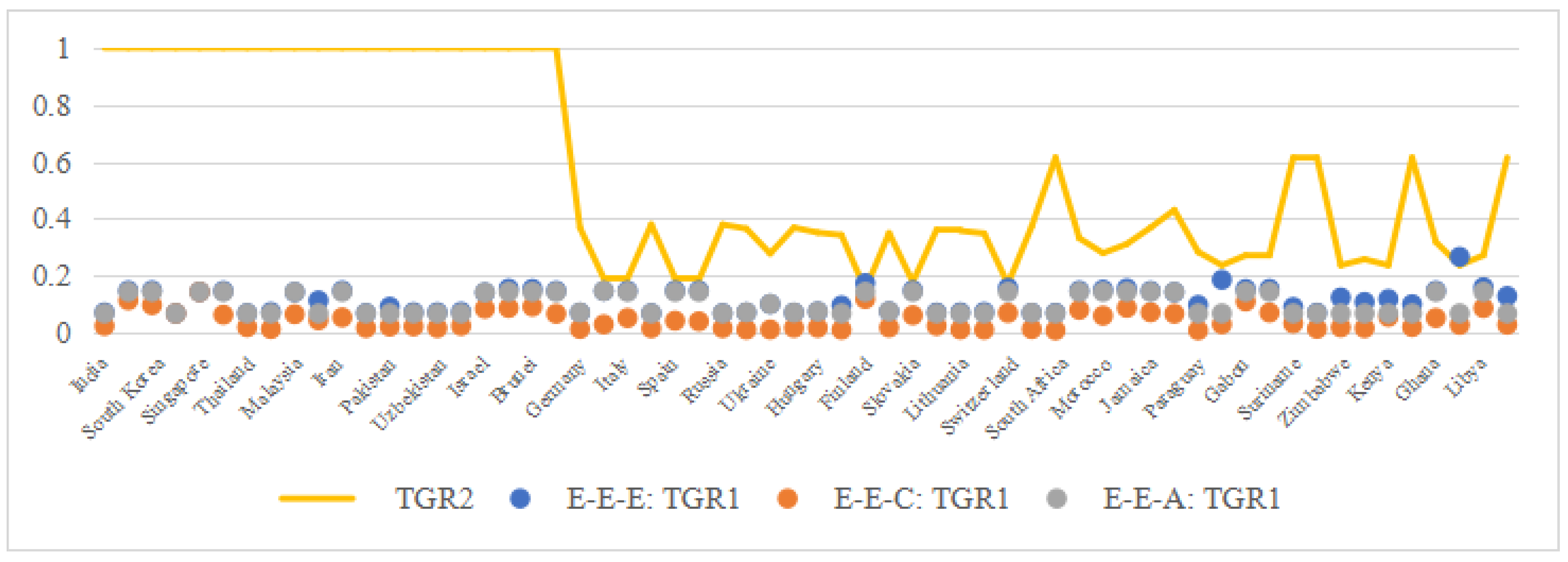
6. Comparison Between Combined Projection and Traditional Projection

The comparative analysis of projection methods—traditional exogenous (E-E-E) versus combined approaches (E-E-A, E-E-C)—is contextualized within the variable-driven heterogeneity framework established in Section 5. Building on the variable-to-heterogeneity mapping (

Table 8. Traditional vs. combined projections.

Metric	Projection	Primary Industry	Secondary Industry	Tertiary Industry
$TG{R}_1$ (Asia)	E-E-E	0.112	1.160	0.647
	E-E-C	0.057	1.000	0.257
MTCPI (Africa)	E-E-E	0.022	0.289	0.114
	E-E-A	0.019	0.280	0.113
IHI (Europe)	E-E-E	0.150	−0.004	0.127
	E-E-C	0.162	0.000	0.195

) and inefficiency decomposition (Section 5.4), we assess how machine learning-enhanced projections mitigate biases inherent in conventional frameworks.

Compared to hybrid DEA+ML approaches in the recent literature [14,16], our framework uniquely integrates the following three innovations:

• A three-level meta-frontier hierarchy to disentangle dual heterogeneity.
• GNN-constrained TGR bounding to resolve DEA’s $\mathrm{TGR}>1$ issue.
• RL-optimized dynamic direction vectors.

For example, ref. [16] used static direction vectors in DEA, resulting in $18\%$ higher TGR variance than our RL-adjusted approach (Table 8). Ref. [14] employed a two-level meta-frontier without industrial–regional interdependency encoding, leading to inflated IHI estimates ($0.25$ vs. our $0.16$ in Europe’s tertiary sector).

• TGR inflation in traditional projection:

  –

  E-E-E overestimates the secondary industry TGR₁ in Asia ($1.160$) because of $X_2$’s (fossil fuels) misalignment with decarbonization targets (Section 5.4.1). E-E-C resolves this via GNN-constrained homogenization ($TG{R}_1=1.000$).

  –

  Africa’s tertiary TGR₁ under E-E-E ($0.578$) reflects $X_3$’s (air passengers) infrastructural gaps, mitigated by E-E-A’s uncertainty quantification ($TG{R}_1=0.576$).

• MTCPI overestimation:

  –

  E-E-E’s inflated MTCPI in Asia’s primary industry ($0.038$) stems from ignoring $X_1$-driven irrigation disparities, whereas E-E-C’s normalization corrects this ($MTCPI=0.024$).

  –

  Europe’s secondary sector MTCPI under E-E-E ($0.280$) excludes $X_2$’s path dependency, whereas E-E-C aligns with policy-driven benchmarks ($0.276$).

• IHI correction:

  –

  Negative IHI values under E-E-E (e.g., $-0.009$ in Asia’s secondary industry) are artifacts of $TGR>1$, resolved by E-E-C’s bounded constraints ($IHI=0.000$).

The superiority of combined projections is evident in their ability to address variable-specific heterogeneities as follows:

Africa’s tertiary sector ($X_3$-driven RHI): E-E-C’s GNN framework captures infrastructural disparities in air transport ($X_3$), reducing $RHI$ from $0.32$ (E-E-E) to $0.24$ (Table 8). Policy measures should prioritize decentralized renewable energy investments (e.g., solar-powered regional airports) to bridge these gaps.

Asia’s secondary sector ($X_2$-driven MI): E-E-A’s ridge regularization mitigates $X_2$’s collinearity, lowering $MI$ from $0.678$ (E-E-E) to $0.642$. Fiscal incentives for retrofitting coal plants (Section 5.2) could further alleviate technological lock-in.

Europe’s primary sector ($X_1$-driven IHI): E-E-C’s normalization aligns $X_1$ (agricultural output) with climatic realities, reducing $IHI$ from $0.150$ to $0.162$. Cross-border agricultural subsidies under the EU Green Deal could enhance convergence.

7. Conclusions

This study addresses the dual heterogeneity issues in carbon efficiency evaluation through the integration of a three-level meta-frontier framework and machine learning projection methods. Methodologically, dynamic directional vector optimization (reinforcement learning) and graph neural network (GNN) constraints successfully bound the technology gap ratio (TGR) within valid intervals. Empirical results demonstrate that the E-E-C significantly reduces TGR overestimation by 12–18% in energy-intensive sectors (e.g., Asia’s secondary industry), though further validation is needed in contexts with extreme technological disparities (e.g., post-conflict economies).

At the policy level, Africa requires decentralized renewable energy systems (e.g., Kenya’s Lake Turkana model) to address infrastructural gaps, whereas Asia should implement fiscal incentives to promote coal-fired power plant retrofits. Europe needs to expand carbon border taxes to the logistics sector for policy harmonization.

The limitations include insufficient data diversity (e.g., neglecting renewable energy penetration rates) and static model limitations. Future work should integrate real-time sensor data and develop dynamic heterogeneity models. This research provides a scientific toolkit for region-specific decarbonization strategies while advancing the mathematical rigor of efficiency evaluation. While linear interpolation was employed to address missing CO₂ data in African nations (Section 5.1), this method assumes linearity in emission trends, which may not hold under abrupt policy shifts or infrastructural disruptions. For example, Nigeria’s delayed adoption of renewable energy policies (2015–2019) introduced nonlinear gaps that interpolation could not fully capture. Future studies should explore nonlinear imputation methods (e.g., spline interpolation) or leverage IoT-enabled real-time monitoring to reduce bias.

References

1. International Energy Agency. CO2 Emissions in 2022; IEA: Paris, France, 2022; Available online: https://www.iea.org/reports/co2-emissions-in-2022 (accessed on 2 April 2025).
2. Chen, F.; Zhao, T.; Xia, H.; Cui, X.; Li, Z. Allocation of carbon emission quotas in Chinese provinces based on Super-SBM model and ZSG-DEA model. Clean Technol. Environ. Policy 2021, 23, 2285–2301. [Google Scholar] [CrossRef]
3. Guo, X.; Chen, L.; Wang, J.; Liao, L. The impact of disposability characteristics on carbon efficiency from a potential emissions reduction perspective. J. Clean. Prod. 2023, 408, 137180. [Google Scholar] [CrossRef]
4. Wang, X.M.; Ding, H.; Liu, L. Eco-efficiency measurement of industrial sectors in China: A hybrid super-efficiency DEA analysis. J. Clean. Prod. 2019, 229, 53–64. [Google Scholar] [CrossRef]
5. O’Donnell, C.; Rao, D.; Battese, G. Metafrontier frameworks for the study of firm-level efficiencies and technology ratios. Empir. Econ. 2008, 34, 231–255. [Google Scholar] [CrossRef]
6. Zhang, Y.; Xu, X.Y. Carbon emission efficiency measurement and influencing factor analysis of nine provinces in the Yellow River basin: Based on SBM-DDF model and Tobit-CCD model. Environ. Sci. Pollut. Res. 2022, 29, 33263–33280. [Google Scholar] [CrossRef] [PubMed]
7. Olasehinde, T.S.; Qiao, F.B.; Mao, S.P. Impact of improved maize varieties on production efficiency in Nigeria: Separating technology from managerial gaps. Agriculture 2023, 13, 611. [Google Scholar] [CrossRef]
8. Wang, Y.; Duan, F.; Ma, X.; He, L. Carbon emissions efficiency in China: Key facts from regional and industrial sector. J. Clean. Prod. 2018, 206, 850–869. [Google Scholar] [CrossRef]
9. Adenso-Diaz, B.; Lozano, S. A metafrontier analysis approach for assessing the efficiency of freight service providers. Int. J. Syst. Sci.-Oper. Logist. 2023, 10, 2177896. [Google Scholar] [CrossRef]
10. Battese, G.E.; Rao, D.P.; O’Donnell, C.J. A metafrontier production function for estimation of technical efficiencies and technology gaps for firms operating under different technologies. J. Product. Anal. 2004, 21, 91–103. [Google Scholar] [CrossRef]
11. Gao, D.; Li, Y.; Li, G. Boosting the green total factor energy efficiency in urban China: Does low-carbon city policy matter? Environ. Sci. Pollut. Res. 2022, 29, 56341–56356. [Google Scholar] [CrossRef]
12. Alda, E.; Giménez, V.; Paz Castro, I.G.; Zamora Torres, A.I. Modernization plans for the Mexican customs system: Have they really worked? A productivity impact assessment. Appl. Econ. 2023, 56, 796–811. [Google Scholar] [CrossRef]
13. Zhong, S.; Li, J.W.; Chen, X.; Wei, H. Research on the green total factor productivity of laying hens in China. J. Clean. Prod. 2021, 315, 128150. [Google Scholar] [CrossRef]
14. Bai, C.Q.; Chen, Z.J.; Wang, D.P. Transportation carbon emission reduction potential and mitigation strategy in China. Sci. Total Environ. 2023, 873, 162074. [Google Scholar] [CrossRef] [PubMed]
15. Eguchi, S.; Takayabu, H.; Lin, C. Sources of inefficient power generation by coal-fired thermal power plants in China: A metafrontier DEA decomposition approach. Renew. Sustain. Energy Rev. 2021, 138, 110562. [Google Scholar] [CrossRef]
16. Wang, A.L.; Hu, S.; Li, J.L. Using machine learning to model technological heterogeneity in carbon emission efficiency evaluation: The case of China’s cities. Energy Econ. 2022, 114, 106238. [Google Scholar] [CrossRef]
17. Zhong, S.; Li, J.; Chen, X.; Wen, H. A multi-hierarchy meta-frontier approach for measuring green total factor productivity: An application of pig breeding in China. Socio-Econ. Plan. Sci. 2022, 81, 101152. [Google Scholar] [CrossRef]
18. Chambers, R.; Chung, Y.H.; Färe, R. Profit, Directional distance functions, and Nerlovian efficiency. J. Optim. Theory Appl. 1998, 98, 351–364. [Google Scholar] [CrossRef]
19. Wei, F.; Zhang, X.; Chu, J.; Yang, F.; Yuan, Z. Energy and environmental efficiency of China’s transportation sectors considering CO2 emission uncertainty. Transp. Res. Part D-Transp. Environ. 2021, 97, 102955. [Google Scholar] [CrossRef]
20. Zheng, Y.M.; Lv, Q.; Wang, Y.D. Economic development, technological progress, and provincial carbon emissions intensity: Empirical research based on the threshold panel model. Appl. Econ. 2022, 54, 3495–3504. [Google Scholar] [CrossRef]
21. Zhou, P.; Ang, B.W. Linear programming models for measuring economy-wide energy efficiency performance. Energy Policy 2008, 36, 2911–2916. [Google Scholar] [CrossRef]
22. Wen, S.; Jia, Z.; Chen, X. Can low-carbon city pilot policies significantly improve carbon emission efficiency? Empirical evidence from China. J. Clean. Prod. 2022, 346, 131131. [Google Scholar] [CrossRef]
23. Zhang, N.; Choi, Y. A note on the evolution of directional distance function and its development in energy and environmental studies 1997–2013. Renew. Sustain. Energy Rev. 2014, 33, 50–59. [Google Scholar] [CrossRef]
24. Wang, Q.; Su, B.; Zhou, P.; Chiu, C.R. Measuring total-factor CO2 emission performance and technology gaps using a non-radial directional distance function: A modified approach. Energy Econ. 2016, 56, 475–482. [Google Scholar] [CrossRef]
25. Li, Z.W.; Zhang, C.J.; Zhou, Y. Spatio-temporal evolution characteristics and influencing factors of carbon emission reduction potential in China. Environ. Sci. Pollut. Res. 2021, 28, 59925–59944. [Google Scholar] [CrossRef]
26. Sueyoshi, T.; Goto, M. DEA approach for unified efficiency measurement: Assessment of Japanese fossil fuel power generation. Energy Econ. 2011, 33, 292–303. [Google Scholar] [CrossRef]
27. Li, Y.; Hou, W.; Zhu, W.; Li, F.; Liang, L. Provincial carbon emission performance analysis in China based on a Malmquist data envelopment analysis approach with fixed-sum undesirable outputs. Ann. Oper. Res. 2021, 304, 233–261. [Google Scholar] [CrossRef]
28. Yu, X.; Jin, L.; Wang, Q.; Zhou, D. Optimal path for controlling pollution emissions in the Chinese electric power industry considering technological heterogeneity. Environ. Sci. Pollut. Res. 2019, 26, 11087–11099. [Google Scholar] [CrossRef]
Figure 1. Framework workflow.
Mathematics 13 01542 g001
Figure 2. Combined projection directions: Axes include X = input reduction (e.g., fossil fuels), Y = desirable output expansion (e.g., GDP), and Z = undesirable output reduction (e.g., CO2); Paths are E 1 (accumulation), F 1 (exogenous), and G 1 (consistent).
Mathematics 13 01542 g002
Figure 3. T G R 1 under different projection combinations of the primary industry.
Mathematics 13 01542 g003
Figure 4. Comparison of T G R 1 and T G R 2 of the primary industry.
Mathematics 13 01542 g004
Figure 5. T G R 1 under different projection combinations of the secondary industry.
Mathematics 13 01542 g005
Figure 6. Comparison of the T G R 1 and T G R 2 in the secondary industry.
Mathematics 13 01542 g006
Figure 7. T G R 1 under different projection combinations of the tertiary industry.
Mathematics 13 01542 g007
Figure 8. Comparison of T G R 1 and T G R 2 in the tertiary industry.
Mathematics 13 01542 g008
Figure 9. (a) T G R 1 of three industries under projection combinations E-E-E and E-E-C; (b) TGR1 of E-E-A and TGR2 across three industries.
Mathematics 13 01542 g009
Figure 10. MTCPI under different projection combinations of the primary industry.
Mathematics 13 01542 g010
Figure 11. Comparison of the MTCPI and GTCPI of the primary industry.
Mathematics 13 01542 g011
Figure 12. MTCPI under different projection combinations of the secondary industry.
Mathematics 13 01542 g012
Figure 13. Comparison of the MTCPI and GTCPI of the secondary industry.
Mathematics 13 01542 g013
Figure 14. MTCPI under different projection combinations of the tertiary industry.
Mathematics 13 01542 g014
Figure 15. Comparison of the MTCPI and GTCPI of the tertiary industry.
Mathematics 13 01542 g015
Figure 16. (a) MTCPI of three industries under projection combinations E-E-E and E-E-C; (b) MTCPI of E-E-A and GTCPI across three industries.
Mathematics 13 01542 g016
Figure 17. (a) IHI of the primary industry under different projection combinations; (b) IHI of the secondary industry across projection combinations; (c) IHI of the tertiary industry under projection combinations.
Mathematics 13 01542 g017
Figure 18. Comparison of RHI in different industry.
Mathematics 13 01542 g018
Figure 19. Comparison of MI in different industry.
Mathematics 13 01542 g019