Incorporating Prior Information in Latent Structures Identification for Panel Data Models

Abstract

In this paper, we explore the latent structures for panel data models in presence of available prior information. The latent structure in panel models allows individuals to be classified into several distinct groups, where the individuals within the same group share the same slope parameters, while the group-specific parameters are heterogeneous. To incorporate the prior information, we design a new alternating direction method of multipliers (ADMM) algorithm based on the pairwise group fused Lasso penalty approach. The asymptotic properties and the convergence of ADMM algorithm are well established. Simulation studies demonstrate the advantages of the proposed method over existing methods in terms of both estimation efficiency and detection accuracy. We illustrate the practical utility of the proposed procedure by analyzing the relationship between electricity consumption and GDP in China.

1. Introduction

Panel data models are widely encountered in many substantial areas in both econometric and statistics. When conducting analyses for panel data, conventional approaches typically assume that the slopes of regressors are completely homogeneous across all individuals [1]. However, such homogeneity assumptions are not in accordance with reality through many practical analyses. See, for example,  [2,3,4], to name a few. From the perspective of model strategy, the complete homogeneity assumption ignores individual-specific heterogeneity, which is quite important in panel data analysis. On the other hand, estimating parameters for each individual separately is feasible for achieving complete heterogeneity, but the estimators and relevant inferences are inefficient or even imprecise, as the time dimension T is usually very short. To strike a balance between completely homogeneous and fully heterogeneous models, a natural way is to assume that the panel units can be classified into several unknown groups, where the members within a group share the same slope parameters, while the slopes across different groups are different. In this way, the convergence rate of estimators changes from $\sqrt{T}$ to $\sqrt{N_{k}T}$, where $N_k$ is the total number of individuals in the kth group. The group structure here is called latent structure [5], and the identification of latent structures is sometimes called homogeneity structure learning [6,7] or subgroup identification [8].

1.1. Literature Review

The existing literature on exploring the latent group structure can be roughly classified into three categories based on different perspectives. First, researchers have found that identifying the latent group can be formulated into a penalization estimation context, such that modern feature selection techniques [9,10] can be employed. A pivotal contribution in this area can be traced back to [5], who developed a novel variant of the Lasso estimator called Classifier-Lasso (C-Lasso). The penalty form of C-Lasso takes an additive-multiplicative form, which forces the parameters of individuals into several groups for a given number of groups. This method had subsequently been extended in various panel models, such as [11,12,13,14]. Recently, ref. [15] proposed a new penalized estimation procedure based on the pairwise adaptive group fused Lasso (PAGFL) penalty, which can automatically identify latent group structures by shrinking the difference in slopes between two individuals towards zero. Compared to C-Lasso, this approach is guaranteed to converge to a unique global minimizer. Second, note that clustering panel individuals into groups is essentially a supervised clustering problem. Hence, the classical K-means algorithm can be adapted to the panel regression framework with group structures with slight modifications. Research in this direction includes [2,16,17]. The third popular approach is based on the sequential binary segmentation algorithm (SBSA) of [18] which was originally designed for structural break detection. Ref. [19] employed the SBSA to detect latent group structures in nonlinear panel models, which consists of two steps: first, sorting the preliminary unconstrained consistent estimators of the regression coefficients, and then performing break point detection. The individuals within adjacent estimated change points therefore form a group. This idea has subsequently been extended by [20,21] to detect the latent structures in spatial dynamic panels and time-varying panels.

These methods make important contributions but often ignore the use of prior information. It is well-known that incorporating prior information in economic and statistical modeling can help improve estimation performance. For example, in the application of predicting clinical measures from neuroimages, ref. [22] proposed a sparse fused group Lasso method that incorporates spatial and group structure information to enhance prediction accuracy. Similarly, ref. [23] detected the sparsity and homogeneity of regression coefficients with imposed prior constraints. To quickly identify clustered patterns in spatial regression and reduce computational burden, ref. [24] built a minimum spanning tree (MST) based on the spatial neighborhood information, and then detected homogeneity in coefficients based on the tree. Along this line, ref. [25] proposed a new MST by leveraging the concept of network topology and the local model similarity, simultaneously. Numerical experiments and real-world data analysis in the literature demonstrated that incorporating more prior information can achieve better estimation and clustering efficiency.

In panel data analysis, researchers often have access to prior information before economic modeling, such as existing research conclusions or objective geographic information. For example, ref. [15] used the preliminary individual-specific estimator to construct the data-adaptive weights in PAGFL. The adaptive weights can be regarded as the indicator for similarity among units that implies the likelihood of two units being in the same group. One important example, which is closely related to this work, is [26], who extended the idea of [6] and exploited a panel-CARDS algorithm. This method first sorts all individuals based on a preliminary estimator, and then constructs an ordered partition set for the individuals. By applying shrinkage estimation between and within the segments, the latent structure can be identified in a data-driven manner. Notably, constructing the rank mapping from the preliminary estimates effectively borrows prior information. Another leading example arises from [2], who studied grouped fixed effects and assumed that some coefficients do not change across individuals. This model setup also posits the prior information that the coefficients of certain regressors are homogeneous across individuals. Hence, as noted by [2] in their supplementary material, adding prior information on the structure of unobserved homogeneity deserves further investigation, and we are currently working on this issue.

1.2. Contributions and Organization

This paper mainly focuses on incorporating the prior information to improve the latent structures detection performance. The contributions are as follows. First, we provide a general prior information framework that can be represented as a constrained region for regression coefficients for panel models. To  identify the latent group structure and utilize the prior information, we develop a novel penalized estimation scheme based on the concave pairwise fusion penalty combining the constraint information. Second, due to the restrictions imposed by the prior constraint, traditional numerical optimization algorithms cannot be directly applied here. To implement the proposed approach, we further design an alternating direction method of multipliers (ADMM) algorithm [27] for solving the constrained fused Lasso problem. The ADMM algorithm is straightforward and easy to implement using free software such as R. Additionally, we have developed a new R package phpadmm to facilitate the estimation procedures described in this paper, which is available upon request. Third, we also demonstrate the convergence property of the ADMM algorithm and the asymptotic results for the estimators. We validate the theoretical results through simulation studies and real-world application. Fourth, we apply the proposed latent structures detection procedure to investigate the relationship between electricity consumption and GDP in China, a significant topic that has garnered considerable interest in the field of energy economics, and find four subgroups among the 30 provinces.

The remainder of the paper is structured as follows. We illustrate the proposed ADMM estimation method in Section 2. The  convergence of the algorithm and the asymptotic theory for the estimators are examined in Section 3. Section 4 compares the finite sample performance of different methods. We investigate the effect of electricity consumption on GDP using proposed methodology in Section 5. Section 6 concludes the paper. The proofs and additional testing procedure are given in the Appendix.

Notation. Throughout this paper, we adopt the following notations. Denote ${\mathbf{0}}_m$ as a $m\times 1$ zero vector, ${\mathbf{1}}_m$ as a $m\times 1$ unit vector, and ${\mathbf{I}}_m$ as a $m\times m$ identity matrix. Let $〈\mathbf{a},\mathbf{b}〉={\mathbf{a}}^{\mathrm{T}}\mathbf{b}$ be the inner product of two vector $\mathbf{a}$ and $\mathbf{b}$ with the same dimension. For an $m\times n$ matrix $\mathbf{A}={({\mathbf{a}}_1,\cdots ,{\mathbf{a}}_n)}^{\mathrm{T}}$, we denote its transpose as ${\mathbf{A}}^{\mathrm{T}}$ and $\mathrm{vec}\left(\mathbf{A}\right)={({\mathbf{a}}_1^{\mathrm{T}},\cdots ,{\mathbf{a}}_n^{\mathrm{T}})}^{\mathrm{T}}$. Throughout this paper, a superscript zero on any quantity refers to the corresponding true quantity, which is a fixed number, vector or matrix.

2. Model and Proposed Estimation Method

2.1. Panel Heterogeneity with Prior Constraint Information

Let $y_{it}$ be the real-valued dependent variable and ${\mathbf{x}}_{it}={(x_{it,1},\cdots ,x_{it,p})}^{\top }$ a $p\times 1$ vector of regressors for $i=1,\cdots ,N$ and $t=1,\cdots ,T$, where i and t index the individual and time respectively. We consider the following linear panel model with grouped latent structures pattern:

$$y_{it}={\mu }_i+{\mathbf{x}}_{it}^T{\mathit{\beta }}_i^0+{ϵ}_{it},i=1,\cdots ,N;t=1,\cdots ,T,$$

(1)

where ${\mu }_i$ is the fixed individual effect for the ith individual, ${ϵ}_{it}$ is error term with mean zero, and ${\mathit{\beta }}_i^0$ is a $p\times 1$ vector of unknown coefficients for the ith individual. The set of coefficients $\{{\mathit{\beta }}_1^0,\cdots ,{\mathit{\beta }}_N^0\}$ admits the following latent grouping structure

$${\mathit{\beta }}_i^0=\left\{\begin{array}{cc}{\mathit{\alpha }}_1^0,& \mathrm{if} i\in G_1^0\\ ⋮& ⋮\\ {\mathit{\alpha }}_{K_0}^0& \mathrm{if} i\in G_{K_0}^0\end{array}\right.$$

(2)

where $K_0$ is an unknown integer, ${\mathit{\alpha }}_l^0\ne {\mathit{\alpha }}_k^0$ for any $l\ne k$, and ${\mathit{\alpha }}_k$ represents the common slope parameters for the kth subgroup. The set ${\mathcal{G}}^0=\{G_1^0,\cdots ,G_K^0\}$ forms a partition of $\{1,\cdots ,N\}$ and $G_l^0\cap G_k^0=\varnothing$ for any $l\ne k$.

Let $\mathcal{B}={({\mathit{\beta }}_1,\cdots ,{\mathit{\beta }}_N)}^{\mathrm{T}}$ be a $K\times p$ coefficient matrix, and let $\mathit{\beta }=\mathrm{vec}\left(\mathcal{B}\right)$. In this paper, we assume that the prior information can be formulated as a constrained region, i.e.,

$$\mathit{\beta }\in \mathcal{C},$$

(3)

where $\mathcal{C}$ is a non-empty convex set, which is quite general. For example, in a cross-province panel data analysis, one may consider that the provinces in neighboring regions are more likely to belong to the same group. We can incorporate geographical information into $\mathcal{C}$. Similarly, in financial studies, the financial returns of similar industry sectors tend to share the same scores on the common factors. In addition, when $\mathcal{C}=\{\mathit{\beta }:\mathit{\beta }\in {\mathbb{R}}^{Np}\}$, group identification in (2) simplifies to the no-prior information situation, which has been discussed by e.g., [5,12,13]. The convex set $\mathcal{C}$ is user-specified that can include equality constraints, inequality constraints, or other constrained forms depending on practical considerations. To enhance the readability of this paper, we summarize the key notations in

Table 1. The notations in our working model.

	Notation	Illustration
Observed quantities	$y_{it}$	the univariate response variable
	${\mathbf{x}}_{it}$	the $p\times 1$ explanatory variables
	$\mathcal{C}$	the prior constraint information set
	N	the number of all individuals
	T	the number of observations for each individual
Unknown parameters	${\mu }_i$	the fixed effect of the ith individual
	${\mathit{\beta }}_i$	the slope of the ith individual
	$\mathcal{G}$	the latent group structures
	$G_k$	the membership of the kth group
	${\mathit{\alpha }}_k$	the common slope of the kth group
	K	the number of latent groups

.

Prior information is typically known and significant, especially in the context of this paper. As mentioned earlier, several existing methods has utilized the prior information in identifying the latent group structures in panel models, including the ordering-based method [26], and the adaptive weights in the group fused Lasso penalty [15]. In essence, these two methods both make use of the distance between any two units’ initial slope estimators. In contrast, our method generalizes the definition of prior information including both the equality and inequality constraints. We summarize the differences between the existing works and our framework about prior information in

Table 2. Comparison with other literature in latent structures identification for panel models.

Methods	Penalty Forms	Prior Information
C-Lasso [5]	${\sum }_{i=1}^N{\prod }_{k=1}^K\parallel {\mathit{\beta }}_i-{\mathit{\alpha }}_k\parallel$	No prior information
Panel-CARDS [26]	${\sum }_{l=1}^{L-1}{\sum }_{i\in B_l,j\in B_{l+1}}{p}_{{\gamma }_1}(\parallel {\mathit{\beta }}_i-{\mathit{\beta }}_j\parallel )+$	An ordered segmentation
	${\sum }_{l=1}^L{\sum }_{i,j\in B_l}{p}_{{\gamma }_2}(\parallel {\mathit{\beta }}_i-{\mathit{\beta }}_j\parallel )$	$\{B_1,\cdots ,B_L\}$
PAGFL [15]	${\sum }_{1\le i<j\le N}{\ddot{w}}_{ij}\parallel {\mathit{\beta }}_i-{\mathit{\beta }}_j\parallel$	Adaptive weights ${\ddot{w}}_{ij}$’s
Our work	${\sum }_{1\le i<j\le N}{p}_{\gamma }(\parallel {\mathit{\beta }}_i-{\mathit{\beta }}_j{\parallel }_1)+{\mathbb{I}}_{\mathcal{C}}\left(\mathit{\beta }\right)$	A convex set $\mathcal{C}$

. Effectively utilizing this prior information can enhance both homogeneity detection and parameter estimation accuracy. Our objective in this paper is to explore how to incorporate these prior constraints (3) into the process of detecting homogeneity.

2.2. A Regularized Approach

To detect homogeneity in panel data models, one may utilize the K-means clustering method, as demonstrated by [2,8], or the binary segmentation method proposed by [28]. However both methods struggle to incorporate prior information effectively. In  this paper, we consider a regularized approach with a concave pairwise fusion penalty to detect homogeneity in model (1). This method was firstly applied in [29] for subgroup analysis and has been extensively employed in various fields, such as precision medicine. After concentrating out the fixed effects, the objective function can be represented as

$$\begin{array}{c}\mathcal{L}(\mathit{\beta };\gamma )={\displaystyle \frac{1}{2NT}}\sum _{i=1}^N\sum _{t=1}^T{({\tilde{y}}_{it}-{\tilde{\mathbf{x}}}_{it}^{\top }{\mathit{\beta }}_i)}^2+\sum _{i<j}{p}_{\gamma }(\parallel {\mathit{\beta }}_i-{\mathit{\beta }}_j{\parallel }_1)\\ s.t.\mathit{\beta }\in \mathcal{C}\end{array}$$

(4)

where ${\tilde{\mathbf{x}}}_{it}={\mathbf{x}}_{it}-{\overline{\mathbf{x}}}_i$ and ${\tilde{y}}_{it}=y_{it}-{\overline{y}}_i$ in which ${\overline{\mathbf{x}}}_i={\displaystyle \frac{1}{T}}{\sum }_{t=1}^T{\mathbf{x}}_{it}$ and ${\overline{y}}_i={\displaystyle \frac{1}{T}}{\sum }_{t=1}^T{y}_{it}$, $p_{\gamma }(·)$ is penalty functions and $\gamma >0$ is a tuning parameters that control the degree of penalty on $\parallel {\mathit{\beta }}_i-{\mathit{\beta }}_j{\parallel }_1$. There are a total of ${\displaystyle \frac{N(N-1)}{2}}$ terms in ${\sum }_{i<j}{p}_{\gamma }(\parallel {\mathit{\beta }}_i-{\mathit{\beta }}_j{\parallel }_1)$, which encourages shrinkages of the pairwise differences in slopes for any two subjects. This regularized adjustment can identify the latent homogeneous structures for the coefficients $\mathit{\beta }$. Ref. [30] pointed out that the non-convex penalties $p_{\gamma }(·)$ should satisfy four conditions, and the smoothly clipped absolute deviation (SCAD) [9] and minimax concave (MCP) [31] penalties are adequate choices.

To further incorporate the prior constraint condition (3), we introduce a new regularized term and rewrite the objective function (4) as

$$\tilde{\mathcal{L}}={\displaystyle \frac{1}{2NT}}\sum _{i=1}^N\sum _{t=1}^T{({\tilde{y}}_{it}-{\tilde{\mathbf{x}}}_{it}^{\top }{\mathit{\beta }}_i)}^2+\sum _{i<j}{p}_{\gamma }(\parallel {\mathit{\beta }}_i-{\mathit{\beta }}_j{\parallel }_1)+{\mathbb{I}}_{\mathcal{C}}\left(\mathit{\beta }\right)$$

(5)

where ${\mathbb{I}}_{\mathcal{C}}(·)$ is an indicator function for $\mathit{\beta }$, equaling a constant when $\mathit{\beta }$ belongs to $\mathcal{C}$ and $+\infty$ otherwise. It should be noted that directly minimizing the Equation (5) is computationally challenging, since the SCAD and MCP penalties are not convex, and the pairwise fusion penalization term is non-separable concerning ${\mathit{\beta }}_i$ in the estimation. To achieve computational feasibility, we formally propose an ADMM algorithm to minimize (5).

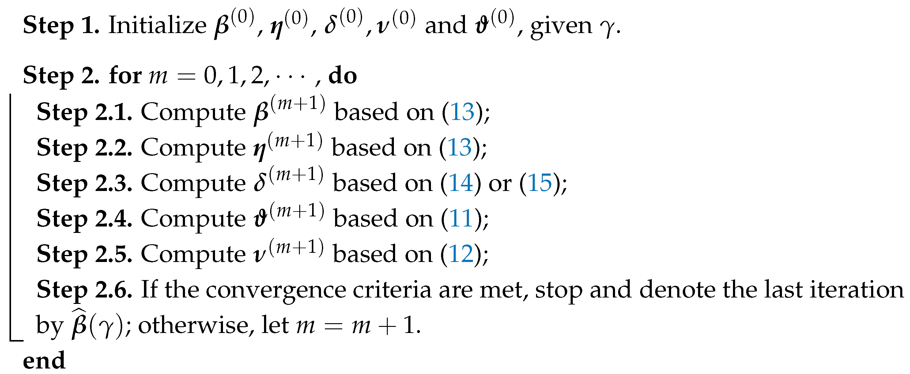
2.3. ADMM Implementation

ADMM algorithm is an optimization algorithm that is particularly useful for solving optimization problems with specific structures, such as those involving separable or block-separable objective functions [27]. The key idea of the ADMM algorithm is to decompose a global optimization problem that is hard to solve into several small pieces that can be solved more easily. In terms of our optimization problem, following the principle of ADMM, we first introduce two sets of auxiliary parameters ${\mathit{\delta }}_{ij}={\mathit{\beta }}_i-{\mathit{\beta }}_j$ and ${\mathit{\eta }}_i={\mathit{\beta }}_i$ to reparameterize the objective function (5) as a constrained optimization problem

$$\begin{array}{c}\tilde{\mathcal{L}}(\mathit{\beta },\mathit{\delta })={\displaystyle \frac{1}{2NT}}\sum _{i=1}^N\sum _{t=1}^T{({\tilde{y}}_{it}-{\tilde{\mathbf{x}}}_{it}^{\top }{\mathit{\beta }}_i)}^2+\sum _{i<j}{p}_{\gamma }(\parallel {\mathit{\delta }}_{ij}{\parallel }_1)+{\mathbb{I}}_{\mathcal{C}}\left(\mathit{\eta }\right)\\ s.t.\left\{\begin{array}{c}{\mathit{\beta }}_i-{\mathit{\beta }}_j-{\mathit{\delta }}_{ij}=\mathbf{0}\hfill \\ \mathit{\beta }-\mathit{\eta }=\mathbf{0}\hfill \end{array}\right.\end{array}$$

(6)

where $\mathit{\delta }={({\mathit{\delta }}_{ij}^{\mathrm{T}},i<j)}^{\mathrm{T}}$ and $\mathit{\eta }={({\mathit{\eta }}_1^{\mathrm{T}},\cdots ,{\mathit{\eta }}_N^{\mathrm{T}})}^{\mathrm{T}}$. To solve (6), we use the ADMM algorithm to solve the following augmented Lagrangian function

$$\begin{array}{ccc}\hfill Q(\mathit{\beta },\mathit{\eta },\mathit{\delta },\mathit{\nu },\mathit{\vartheta })& =& \tilde{L}(\mathit{\beta },\mathit{\delta })+\sum _{i<j}〈{\mathit{\nu }}_{ij},{\mathit{\beta }}_i-{\mathit{\beta }}_j-{\mathit{\delta }}_{ij}〉+{\displaystyle \frac{{\rho }_2}{2}}\sum _{i<j}{\parallel {\mathit{\beta }}_i-{\mathit{\beta }}_j-{\mathit{\delta }}_{ij}\parallel }^2\hfill \\ \hfill & & +{\mathbb{I}}_{\mathcal{C}}\left(\mathit{\eta }\right)+\sum _{j=1}^N〈{\mathit{\vartheta }}_j,{\mathit{\beta }}_j-{\mathit{\eta }}_j〉+{\displaystyle \frac{{\rho }_1}{2}}\sum _{j=1}^N{\parallel {\mathit{\beta }}_j-{\mathit{\eta }}_j\parallel }^2\hfill \end{array}$$

(7)

where $\mathit{\nu }={({\mathit{\nu }}_{ij}^{\mathrm{T}},i<j)}^{\mathrm{T}}$, $\mathit{\vartheta }={({\mathit{\vartheta }}_j^{\mathrm{T}},\cdots ,{\mathit{\vartheta }}_N^{\mathrm{T}})}^{\mathrm{T}}$ are Lagrange multipliers, and ${\rho }_1$, ${\rho }_2$ are two fixed augmented parameters. The ADMM algorithm has the advantage of decomposing (7) into several manageable subsets. Along this line, we consider alternating minimization for each block of parameters $\mathit{\beta },\mathit{\eta },\mathit{\delta },\mathit{\vartheta }$ and $\mathit{\nu }$. Specifically, given the current values at the mth iteration, denoted as $({\mathit{\beta }}^{\left(m\right)},{\mathit{\eta }}^{\left(m\right)},{\mathit{\delta }}^{\left(m\right)},{\mathit{\vartheta }}^{\left(m\right)},{\mathit{\nu }}^{\left(m\right)})$, the ADMM computation at the $(m+1)$th iteration proceeds as follows:

$$\begin{array}{ccc}\hfill {\mathit{\beta }}^{(m+1)}& =& arg\underset{\mathit{\beta }}{min}Q(\mathit{\beta },{\mathit{\eta }}^{\left(m\right)},{\mathit{\delta }}^{\left(m\right)},{\mathit{\vartheta }}^{\left(m\right)},{\mathit{\nu }}^{\left(m\right)}),\hfill \end{array}$$

(8)

$$\begin{array}{ccc}\hfill {\mathit{\eta }}^{(m+1)}& =& arg\underset{\mathit{\eta }}{min}Q({\mathit{\beta }}^{(m+1)},\mathit{\eta },{\mathit{\delta }}^{\left(m\right)},{\mathit{\vartheta }}^{\left(m\right)},{\mathit{\nu }}^{\left(m\right)}),\hfill \end{array}$$

(9)

$$\begin{array}{ccc}\hfill {\mathit{\delta }}^{(m+1)}& =& arg\underset{\mathit{\delta }}{min}Q({\mathit{\beta }}^{(m+1)},{\mathit{\eta }}^{(m+1)},\mathit{\delta },{\mathit{\vartheta }}^{\left(m\right)},{\mathit{\nu }}^{\left(m\right)}),\hfill \end{array}$$

(10)

$$\begin{array}{ccc}\hfill {\mathit{\vartheta }}^{(m+1)}& =& {\mathit{\vartheta }}^{\left(m\right)}+{\rho }_1\left({\mathit{\beta }}^{(m+1)}\right)-{\mathit{\eta }}^{(m+1)}),\hfill \end{array}$$

(11)

$$\begin{array}{ccc}\hfill {\mathit{\nu }}^{(m+1)}& =& {\mathit{\nu }}^{\left(m\right)}+{\rho }_2(\mathsf{\Omega }{\mathit{\beta }}^{(m+1)}-{\mathit{\delta }}^{(m+1)}).\hfill \end{array}$$

(12)

For the first minimization problem in (8), ${\mathit{\beta }}^{(m+1)}$ is the minimizer of

$$\begin{array}{cc}\hfill H_{\rho }\left(\mathit{\beta }\right)=& {\displaystyle \frac{1}{2NT}}\sum _{i=1}^N\sum _{t=1}^T{({\tilde{y}}_{it}-{\tilde{\mathbf{x}}}_{it}^{\top }{\mathit{\beta }}_i)}^2+{\displaystyle \frac{{\rho }_2}{2}}\sum _{i<j}{\parallel {\mathit{\beta }}_i-{\mathit{\beta }}_j-{\mathit{\delta }}_{ij}^{\left(m\right)}+{\rho }_2^{-1}{\mathit{\nu }}_{ij}^{\left(m\right)}\parallel }^2\hfill \\ \hfill & +{\displaystyle \frac{{\rho }_1}{2}}\sum _{j=1}^N{\parallel {\mathit{\beta }}_j-{\mathit{\eta }}_j^{\left(m\right)}+{\rho }_1^{-1}{\mathit{\vartheta }}_j^{\left(m\right)}\parallel }^2+\mathrm{constant}.\hfill \end{array}$$

By simple algebraic manipulation, we can rewrite it in matrix form

$$\begin{array}{cc}\hfill H_{\rho }\left(\mathit{\beta }\right)=& {\displaystyle \frac{1}{2NT}}\parallel \tilde{y}-\tilde{\mathbf{x}}{\mathit{\beta }\parallel }^2+{\displaystyle \frac{{\rho }_2}{2}}{\parallel \mathbf{D}\mathit{\beta }-{\mathit{\delta }}^{\left(m\right)}+{\rho }_2^{-1}{\mathit{\nu }}^{\left(m\right)}\parallel }^2\hfill \\ \hfill & +{\displaystyle \frac{{\rho }_1}{2}}{\parallel \mathit{\beta }-{\mathit{\eta }}^{\left(m\right)}+{\rho }_1^{-1}{\mathit{\vartheta }}^{\left(m\right)}\parallel }^2+\mathrm{constant},\hfill \end{array}$$

where $\tilde{y}={({\tilde{y}}_1^{\mathrm{T}},\cdots ,{\tilde{y}}_N^{\mathrm{T}})}^{\mathrm{T}}$ is a $NT\times 1$ vector with ${\tilde{y}}_i={({\tilde{y}}_{i1},\cdots ,{\tilde{y}}_{iT})}^{\mathrm{T}}$, $\tilde{\mathbf{x}}=\mathrm{diag}({\tilde{\mathbf{x}}}_1,\cdots ,{\tilde{\mathbf{x}}}_N)$ is a $NT\times Np$ matrix with ${\tilde{\mathbf{x}}}_i={({\tilde{\mathbf{x}}}_{i1},\cdots ,{\tilde{\mathbf{x}}}_{iT})}^{\mathrm{T}}$, and $\mathbf{D}:=\mathcal{E}\otimes {\mathbf{I}}_p$ is a ${\displaystyle \frac{N(N-1)}{2}}p\times Np$ matrix, where ⊗ represents the Kronecker product, $\mathcal{E}={\{({\mathbf{e}}_i-{\mathbf{e}}_j),i<j\}}_{{\displaystyle \frac{N(N-1)}{2}}\times N}^{\top }$ and ${\mathbf{e}}_i$ is the $N\times 1$ vector with one at the ith component, and zeros elsewhere. Notably, the minimizer has a closed-form solution:

$$\begin{array}{ccc}\hfill {\mathit{\beta }}^{(m+1)}& =& {\left({\displaystyle \frac{1}{NT}}{\tilde{\mathbf{x}}}^{\mathrm{T}}\tilde{\mathbf{x}}+{\rho }_1{\mathbf{I}}_{Np}+{\rho }_2{\mathbf{D}}^{\mathrm{T}}\mathbf{D}\right)}^{-1}\hfill \\ & \times & \left\{{\displaystyle \frac{1}{NT}}{\tilde{\mathbf{x}}}^{\top }y+{\rho }_1({\mathit{\eta }}^{\left(m\right)}-{\rho }_1^{-1}{\mathit{\vartheta }}^{\left(m\right)})+{\rho }_2\mathbf{D}({\mathit{\delta }}^{\left(m\right)}-{\rho }_2^{-1}{\mathit{\nu }}^{\left(m\right)})\right\}.\hfill \end{array}$$

For ${\mathit{\eta }}^{(m+1)}$ in (9), it is actually a standard convex optimization problem, since we only need to minimize

$${\displaystyle \frac{{\rho }_1}{2}}\parallel {\mathit{\xi }}_j^{\left(m\right)}-{\mathit{\eta }}_j\parallel +{\mathbb{I}}_{\mathcal{C}}\left({\mathit{\eta }}_j\right)$$

(13)

where ${\mathit{\xi }}_j^{\left(m\right)}={\mathit{\beta }}_j^{(m+1)}+{\rho }_1^{-1}{\mathit{\vartheta }}_j^{\left(m\right)}$. In practical implementation, we employ the quadratic programming algorithm by the R function “solve.QP” available from the package quadprog.

For ${\mathit{\delta }}^{(m+1)}$ in (10), by discarding the terms that are independent of $\mathit{\delta }$, we just need to minimize

$${\displaystyle \frac{{\rho }_2}{2}}\parallel {\mathit{\zeta }}_{ij}^{\left(m\right)}-{\mathit{\delta }}_{ij}{\parallel }^2+p_{\gamma }(\parallel {\mathit{\delta }}_{ij}{\parallel }_1)$$

where ${\mathit{\zeta }}_{ij}^{\left(m\right)}={\mathit{\beta }}_i^{(m+1)}-{\mathit{\beta }}_j^{(m+1)}+{\rho }_2^{-1}{\mathit{\nu }}_{ij}^{\left(m\right)}$. For the MCP with $\gamma >1/{\rho }_1$, the updated ${\mathit{\delta }}^{(m+1)}$ has a closed-form solution

$${\mathit{\delta }}_{ij}^{\left(m\right)}=\left\{\begin{array}{cc}{\displaystyle \frac{S({\mathit{\zeta }}_{ij}^{\left(m\right)},\lambda /{\rho }_1)}{1-1/\left(\gamma {\rho }_1\right)}}& \mathrm{if} \parallel {\mathit{\zeta }}_{ij}^{\left(m\right)}\parallel \le \gamma \lambda ,\\ {\mathit{\zeta }}_{ij}^{\left(m\right)}& \mathrm{if} \parallel {\mathit{\zeta }}_{ij}^{\left(m\right)}\parallel >\gamma \lambda .\end{array}\right.$$

(14)

For the SCAD penalty with $\gamma >1/{\rho }_1+1$, the update is given by

$${\mathit{\delta }}_{ij}^{\left(m\right)}=\left\{\begin{array}{cc}S({\mathit{\zeta }}_{ij}^{\left(m\right)},\lambda /{\rho }_1)& \mathrm{if} \parallel {\mathit{\zeta }}_{ij}^{\left(m\right)}\parallel \le \lambda +\lambda /{\rho }_1,\\ {\displaystyle \frac{S({\mathit{\zeta }}_{ij}^{\left(m\right)},\gamma \lambda /\left({\rho }_1(\gamma -1)\right))}{1-1/\left(\gamma {\rho }_1\right)}}& \mathrm{if} \lambda +\lambda /{\rho }_1<\parallel {\mathit{\zeta }}_{ij}^{\left(m\right)}\parallel \le \gamma \lambda ,\\ {\mathit{\zeta }}_{ij}^{\left(m\right)}& \mathrm{if} \parallel {\mathit{\zeta }}_{ij}^{\left(m\right)}\parallel >\gamma \lambda .\end{array}\right.$$

(15)

where $S(z,t)={(1-t/\parallel z\parallel )}_{+}z$ is the groupwise soft-thresholding operator with ${\left(x\right)}_{+}=x$ if $x>0$ and 0 otherwise.

As suggested by [27], a reasonable termination criterion for an ADMM algorithm is that both the primal and dual residuals are sufficiently small. In this paper, the primal and dual residuals are defined as

$$\parallel {\mathbf{r}}_1^{(m+1)}{\parallel }^2=\parallel \mathsf{\Omega }{\mathit{\beta }}^{(m+1)}-{\mathit{\delta }}^{(m+1)}{\parallel }^2,\parallel {\mathbf{r}}_2^{(m+1)}{\parallel }^2={\parallel {\mathit{\beta }}^{(m+1)}-{\mathit{\eta }}^{(m+1)}\parallel }^2$$

(16)

and

$$\parallel {\mathbf{s}}_1^{(m+1)}{\parallel }^2=\parallel {\rho }_1({\mathit{\eta }}^{(m+1)}-{\mathit{\eta }}^{\left(m\right)}){\parallel }^2,\parallel {\mathbf{s}}_2^{(m+1)}\parallel =\parallel {\rho }_2\mathsf{\Omega }({\mathit{\delta }}^{(m+1)}-{\mathit{\delta }}^{(m+1)}){\parallel }^2,$$

(17)

respectively. When ${lim}_{m\to \infty }{\parallel {\mathbf{r}}_k^{\left(m\right)}\parallel }^2\le e^{\mathrm{primal}}$ for $k=1,2$ and ${lim}_{m\to \infty }{\parallel {\mathbf{s}}_1^{\left(m\right)}+{\mathbf{s}}_2^{\left(m\right)}\parallel }^2\le e^{\mathrm{dual}}$ hold, where $e^{\mathrm{primal}}$ and $e^{\mathrm{dual}}$ are pre-specified feasible primal and dual tolerances, we stop the iteration. We summarize the above procedures in Algorithm 1.

Algorithm 1: ADMM algorithm for panel data models with prior constraints

2.4. Initial Values and Tuning Parameter

In nonconvex optimization, selecting an appropriate initialization for parameters is crucial, because this will not only produce an optimal solution but also significantly accelerate the iterations. As proposed by [26], we set the initial values for $\mathit{\beta }$ as the estimators without the latent group structure, that is

$$L_{NT}\left(\mathit{\beta }\right)={\displaystyle \frac{1}{2NT}}\sum _{i=1}^N\sum _{t=1}^T{({\tilde{y}}_{it}-{\tilde{\mathbf{x}}}_{it}^{\top }{\mathit{\beta }}_i)}^2.$$

Solve the optimization problem yields the least square estimates

$${\mathit{\beta }}_i^{\left(0\right)}={\left({\displaystyle \frac{1}{T}}\sum _{t=1}^T{\tilde{\mathbf{x}}}_{it}{\tilde{\mathbf{x}}}_{it}^{\mathrm{T}}\right)}^{-1}\left({\displaystyle \frac{1}{T}}\sum _{t=1}^T{\tilde{\mathbf{x}}}_{it}{\tilde{y}}_{it}\right),$$

for $i=1,\cdots ,N$. Then, set ${\mathit{\delta }}_{ij}^{\left(0\right)}={\mathit{\beta }}_i^{\left(0\right)}-{\mathit{\beta }}_j^{\left(0\right)}$, ${\mathit{\eta }}_i^{\left(0\right)}={\mathit{\beta }}_i^{\left(0\right)}$, ${\mathit{\vartheta }}^{\left(0\right)}=\mathbf{0}$, and ${\mathit{\nu }}^{\left(0\right)}=\mathbf{0}$. The question arises regarding how to determine the tuning parameters ${\rho }_1$, ${\rho }_2$ and $\lambda$. Following [29], we set ${\rho }_1={\rho }_2=1$ and $\lambda =3$.

The selection of $\gamma$ is particularly important, since the performance of group structures identification depends on $\gamma$. Following the strategy of [5], we minimize the following BIC-type criterion function:

$$\mathrm{IC}\left(\gamma \right)=log\left({\sigma }_{NT}^2\left(\gamma \right)\right)+pK\left(\gamma \right){\psi }_{NT}$$

(18)

where ${\sigma }_{NT}^2\left(\gamma \right)=L_{NT}\left(\mathit{\beta }\left(\gamma \right)\right)$ is the sum of squared residuals, and $K\left(\gamma \right)$ denotes the number of groups corresponding to $\gamma$. Here, the positive constant ${\psi }_{NT}$ that depends on N and T serve as a balance between the degrees of freedom and the model fitting errors. To select the optimal $\gamma$, define a grid of points ${\gamma }_{min}={\gamma }_0<\cdots <{\gamma }_W={\gamma }_{max}$ with equal spacing. To speed up the computation, we employ the warm start strategy. Specifically, for each $\gamma \in \{{\gamma }_0,\cdots ,{\gamma }_W\}$, we compute the solution path $\widehat{\mathit{\beta }}\left({\gamma }_w\right)$ under the initial value $\widehat{\mathit{\beta }}\left({\gamma }_{w-1}\right)$. The optimal value for $\gamma$ is defined as $\widehat{\gamma }=arg{min}_{{\gamma }_w,w=0,\cdots ,W}\mathrm{IC}\left({\gamma }_w\right)$.

3. Theoretical Analysis

In this section, we mainly discuss the the convergence of the ADMM Algorithm 1, and establish the asymptotic property of the proposed estimator.

3.1. Convergence of the Algorithm

Under some mild conditions, the convergence of the ADMM algorithm can be guaranteed. For the iterated sequence $\{{\mathit{\beta }}^{\left(m\right)},{\mathit{\eta }}^{\left(m\right)},{\mathit{\delta }}^{\left(m\right)},{\mathit{\vartheta }}^{\left(m\right)},{\mathit{\nu }}^{\left(m\right)}\}$, there exists a global minimizer $\{{\mathit{\beta }}^{\ast },{\mathit{\eta }}^{\ast },{\mathit{\delta }}^{\ast },{\mathit{\vartheta }}^{\ast },{\mathit{\nu }}^{\ast }\}$ satisfying the first order condition for a stationary point The following proposition illustrates the convergence of Algorithm 1.

Proposition 1. 

Recall the primal and dual residuals defined in (16) and (17). It holds that ${lim}_{m\to \infty }{\parallel {\mathbf{r}}_j^{\left(m\right)}\parallel }^2=0$ for $j=1,2$, and ${lim}_{m\to \infty }{\parallel {\mathbf{s}}_1^{\left(m\right)}+{\mathbf{s}}_2^{\left(m\right)}\parallel }^2=0$ for both SCAD and MCP penalties. Therefore, the sequence ${\{{\mathit{\beta }}^{\left(m\right)},{\mathit{\eta }}^{\left(m\right)},{\mathit{\delta }}^{\left(m\right)},{\mathit{\vartheta }}^{\left(m\right)},{\mathit{\nu }}^{\left(m\right)}\}}_{m=1}^{\infty }$ will approach to an optimal point.

Proposition 1 indicates that Algorithm 1 converges if both the primal feasibility and dual feasibility hold. The proof of this proposition follows a strategy similar to that in [29], and the detailed proof is postponed to the Appendix.

3.2. Asymptotic Property

We now establish the theoretical properties of the penalized estimator. First, we introduce some notations. Let ${\mathbf{x}}_i={({\mathbf{x}}_{i1},\cdots ,{\mathbf{x}}_{iT})}^{\mathrm{T}}$ and $y_i={(y_{i1},\cdots ,y_{in})}^{\mathrm{T}}$. Let ${\mathcal{G}}^{\left(K\right)}=(G_1^{\left(K\right)},\cdots ,G_K^{\left(K\right)})$ be an arbitrary K-partition of $\{1,\cdots ,N\}$. We define

$${\widehat{\sigma }}_{{\mathcal{G}}^{\left(K\right)}}^2={\left(NT\right)}^{-1}\sum _{k=1}^K\sum _{i\in G_k^{\left(K\right)}}\sum _{t=1}^T{\left({\tilde{y}}_{it}-{\tilde{\mathbf{x}}}_{it}^{\mathrm{T}}{\widehat{\mathit{\beta }}}_{i,G_k^{\left(K\right)}}\right)}^2,$$

where ${\widehat{\mathit{\beta }}}_{i,G_k^{\left(K\right)}}=arg{min}_{{\mathit{\beta }}_i}{\left(N_{k}T\right)}^{-1}{\sum }_{i\in G_k^{\left(K\right)}}{\sum }_{t=1}^T{({\tilde{y}}_{it}-{\tilde{\mathbf{x}}}_{it}^{\mathrm{T}}{\mathit{\beta }}_i)}^2$. Denote $N_k$ as the number of elements in the kth group. Define $\rho \left(t\right)={\lambda }^{-1}{p}_{\gamma }(t,\lambda )$ as the scale penalty function and $\rho \prime \left(t\right)=p_{\lambda }^{\prime }\left(\right|t\left|\right)\mathrm{sgn}\left(t\right)$ as its first-order derivative. We then introduce the following assumptions.

Assumption 1. 

(i) $\{({\mathbf{x}}_{it},y_{it}),t=1,\cdots ,T\}$ is stationary strong mixing for each i with mixing coefficients ${\mathit{\alpha }}_i(·)$. $\mathit{\alpha }(·)={max}_i{\mathit{\alpha }}_i(·)$ satisfies $\mathit{\alpha }\left(\tau \right)\le c_{\mathit{\alpha }}{\rho }^{\tau }$ for some constant $c_{\mathit{\alpha }}>0$ and $\rho \in (0,1)$. (ii) The random variables ${\{{\mathbf{x}}_i,y_i\}}_{i=1}^N$ are independent, and ${max}_{i,t}E{\parallel {\mathbf{x}}_{it}\parallel }^{2q}<c_1$ for some constant $c_1<\infty$ and $q>4$. (iii) There exists two positive constants $c_2$ and $c_3$ such that ${min}_{1\le k\le K}{\mu }_{min}\left({\displaystyle \frac{1}{T{N}_k}}{\sum }_{i\in G_k^0}E\left({\tilde{\mathbf{x}}}_i^T{\tilde{\mathbf{x}}}_i\right)\right)\ge c_2$ and ${max}_{1\le i\le N}{\mu }_{max}\left({\displaystyle \frac{1}{T}}E\left({\mathbf{x}}_i^T{\mathbf{x}}_i\right)\right)\le c_3$. (iv) The error term satisfies $E\left({ϵ}_{it}\right)=0$, $E\left({\mathbf{x}}_{it}{ϵ}_{it}\right)=0$ and ${max}_{i,t}E{\left|{ϵ}_{it}\right|}^{2q}<c_1$. (v) $N_k$ either tends to infinity or remains fixed as $T\to \infty$ and $N=O\left(T^2\right)$.

Assumption 2. 

(i) The function $\rho \left(t\right)$ is symmetric, non-decreasing and concave on $[0,\infty )$. It satisfies $\rho \left(0\right)=0$ and is constant for all $t\ge a\lambda$ for some constant $a>0$. (ii) The derivative $\rho \prime \left(t\right)$ satisfies $\rho \prime (0+)=1$ and is continuous except for a finite number of values of t.

Assumption 3. 

(i) There exist positive definite matrices ${\mathsf{\Omega }}_k$ for $k=1,\cdots ,K$ such that ${\displaystyle \frac{1}{T{N}_k}}{\sum }_{i\in G_k^0}{\sum }_{t=1}^T{\tilde{\mathbf{x}}}_{it}{\tilde{\mathbf{x}}}_{it}^{\mathrm{T}}\stackrel{p}{\to }{\mathsf{\Omega }}_k$ as $T\to \infty$ or $(N_k,T)\to \infty$. (ii) Let ${\mathbb{B}}_k={\displaystyle \frac{1}{\sqrt{N_{k}T}}}{\sum }_{i\in G_k^0}{\sum }_{t=1}^{T}E\left({\tilde{\mathbf{x}}}_{it}{ϵ}_{it}\right)$. Then $\sqrt{N_{k}T}{\sum }_{i\in G_k^0}{\sum }_{t=1}^T{\tilde{\mathbf{x}}}_{it}{ϵ}_{it}-{\mathbb{B}}_k\stackrel{d}{\to }N(0,{\mathsf{\Psi }}_k)$ as $T\to \infty$ or $(N_k,T)\to \infty$ where ${\mathbb{B}}_k$ equals $O_p\left(\sqrt{N_k/T}\right)$ if ${\tilde{\mathbf{x}}}_{it}$ is not exogenous and 0 otherwise.

Assumption 4. 

${min}_{1\le \widehat{K}\le K}{inf}_{{\mathcal{G}}^{\left(\widehat{K}\right)}}{\widehat{\sigma }}_{{\mathcal{G}}^{\left(\widehat{K}\right)}}^2\stackrel{p}{\to }{\underline{\sigma }}^2>{\sigma }_0^2$ as $(N,T)\to \infty$ where ${\sigma }_0^2={lim}_{(N,T)\to \infty }$${\left(NT\right)}^{-1}{\sum }_{k=1}^{K_0}{\sum }_{i\in G_k^0}{\sum }_{t=1}^{T}E({\tilde{y}}_{it}-{\tilde{\mathbf{x}}}_{it}^T{\mathit{\beta }}_i^0).$

Assumption 5. 

As ($N,T)\to \infty$, ${\psi }_{NT}\to 0$ and ${\psi }_{NT}T\to \infty$.

Assumption 1(i,ii) imposes some conditions on $\left\{({\mathbf{x}}_{it},y_{it})\right\}$, which are quite common in panel data models. Assumption 1(iii,iv) specifies moment conditions on the regressors ${\mathbf{x}}_{it}$ and the noise term ${ϵ}_{it}$, respectively. Assumption 1(v) allows the number of elements in each group to be finite, which distinguishes it from the conditions set forth in [5]. Assumption 2 is standard for concave penalty functions, such as SCAD and MCP. Assumption 4 is utilized to study the asymptotic normality of the proposed estimators. Finally, Assumptions 4 and 5 are adapted from [5] to demonstrate the classification consistency described in (18).

Once $\widehat{\mathit{\beta }}$ is given, the estimated group pattern can be directly derived by classifying the coefficients ${\widehat{\mathit{\beta }}}_i$’s into groups. We denote $\widehat{K}$ as the estimated number of groups and ${\widehat{\mathit{\alpha }}}_k$ as the common slope shared by the kth group for $k=1,\cdots ,\widehat{K}$. By definition, the estimated group pattern $\widehat{\mathcal{G}}=({\widehat{G}}_1,\cdots ,{\widehat{G}}_{\widehat{K}})$ is given by

$${\widehat{G}}_k=\{i\in \{1,\cdots ,N\}:{\widehat{\mathit{\beta }}}_i={\widehat{\mathit{\alpha }}}_k\}\mathrm{for} k=1,\cdots ,\widehat{K}.$$

We then have the following limiting distribution for ${\widehat{\mathit{\alpha }}}_k$.

Theorem 1. 

Suppose that Assumption 1–3 hold. Then,

$$\sqrt{N_{k}T}({\widehat{\mathit{\alpha }}}_k-{\mathit{\alpha }}_k^0)-{\mathsf{\Omega }}_k^{-1}{\mathbb{B}}_k\stackrel{d}{\to }N(0,{\mathsf{\Omega }}_k^{-1}{\mathsf{\Psi }}_k{\mathsf{\Omega }}_k^{-1})$$

for $k=1,\cdots ,K$ as $T\to \infty$ or $(N_k,T)\to \infty$.

Theorem 1 demonstrates that the group-specific estimator possesses the asymptotic normality properties with a convergence rate of $\sqrt{N_{k}T}$. If the group membership is known, the oracle estimator for $\mathit{\alpha }$ is given by

$${\widehat{\mathit{\alpha }}}_k^{or}={\left(\sum _{i\in G_k^0}{\tilde{\mathbf{x}}}_i^{\mathrm{T}}{\tilde{\mathbf{x}}}_i\right)}^{-1}\left(\sum _{i\in G_k^0}{\tilde{\mathbf{x}}}_i^{\mathrm{T}}{\tilde{y}}_i\right),\mathrm{for} k=1,\cdots ,K.$$

As pointed by [5,26], ${\widehat{\mathit{\alpha }}}_k^{or}$ and ${\widehat{\mathit{\alpha }}}_k$ share similar asymptotic normality. Given the estimated grouping structure $\widehat{\mathcal{G}}$, a post-Lasso version of $\mathit{\alpha }$ is obtained by

$${\widehat{\mathit{\alpha }}}_{{\widehat{G}}_k}={\left(\sum _{i\in {\widehat{G}}_k}{\tilde{\mathbf{x}}}_i^{\mathrm{T}}{\tilde{\mathbf{x}}}_i\right)}^{-1}\left(\sum _{i\in {\widehat{G}}_k}{\tilde{\mathbf{x}}}_i^{\mathrm{T}}{\tilde{y}}_i\right),\mathrm{for} k=1,\cdots ,\widehat{K}.$$

The post-Lasso estimators perform at least as well as the Lasso estimators in terms of convergence rate, but they exhibit a smaller second-order bias, as shown by [32]. It would be interesting to investigate the higher-order asymptotic properties of the post-Lasso estimators within our framework.

We utilize the information criterion defined in (18) to determine the number of groups. The following theorem justifies its asymptotic validity.

Theorem 2. 

Suppose that Assumptions A1–A2 and A4–A5 hold. The information criterion in (18) will select a optimal tuning parameter ${\gamma }^{opt}$ such that the estimated $\widehat{\mathit{\beta }}\left({\gamma }^{opt}\right)$ approaches to the oracle estimator ${\widehat{\mathit{\beta }}}^{or}$ with probability approaching 1, and 

$$P(\widehat{K}\left({\gamma }^{opt}\right)=K)\to 1,\mathrm{as} (N,T)\to \infty .$$

Theorem 2 indicates that under some mild condition, the minimizer of (18) can only be the one that produces the correct number of groups, as N or T or both go to infinity. Since ${\psi }_{NT}$ in the IC (18) plays a crucial role in determining the latent group structures, we follow [5] to pick ${\psi }_{NT}$ by trying a list of candidates. Similar to [26], we find that ${\psi }_{NT}={\displaystyle \frac{1}{2\sqrt{NT}}}$ has fairly good sample performance. The same setting is also aplied in the empirical study.

4. Simulation Studies

In this section, we conduct a series of simulation studies to assess the finite sample performance of the proposed method. We consider the following three data generating processes:

4.1. Basic Setup

DGP 1. The first data setting is similar to the GDP 1 in [5]. Here, the observations $\{(y_{it},{\mathbf{x}}_{it}),i=1,\cdots ,N,t=1,\cdots ,T\}$ are generated from a linear panel model where ${\mathbf{x}}_{it}={(0.2{\mu }_i+e_{it1},0.2{\mu }_i+e_{it2})}^{\mathrm{T}}$ with the fixed effect ${\mu }_i$ following an i.i.d. standard normal distribution across time. The error terms $e_{it1}$ and $e_{it2}$ are i.i.d. standard normal and independent of ${\mu }_i$. The slopes of individuals are divided into three groups with a ratio of $N_1:N_2:N_3=4:3:3$. The true coefficients are

$${\mathcal{B}}_a={\left(\begin{array}{ccc}0.4& 1& 1.6\\ 1.6& 1& 0.4\end{array}\right)}^{\mathrm{T}}.$$

DGP 2. The DGP 2 is similar to the DGP 3 in [26]. In this setting, the coefficients are divided into eight groups, where the first group accounts for 30% of the total individuals and each of the remaining seven groups shares 10% of individuals. The generation for ${\mathbf{x}}_{it}$ is similar to DGP 1. The group-specific coefficients take the values

$${\mathcal{B}}_b={\left(\begin{array}{cccccccc}-4& -3& -2& -1& 1& 2& 3& 4\\ 4& 3& 2& 1& -1& -2& -3& -4\end{array}\right)}^{\mathrm{T}}.$$

DGP 3. In the third DGP, we let ${\mathbf{x}}_{it}={(x_{it1},x_{it2},x_{it3})}^{\mathrm{T}}$ and $x_{itk}=0.2{\mu }_i+e_{itk}$ for $k=1,2,3$. Individuals are also divided into three groups with a ratio of $N_1:N_2:N_3=3:4:3$. The true parameter values for each group are

$${\mathcal{B}}_c={\left(\begin{array}{ccc}0.6& 0.6& 0.6\\ 1.5& 1& 0.5\\ -1& 0& 1\end{array}\right)}^{\mathrm{T}}$$

The constraint set for each DGP includes both equality or inequality constraints, which are described as follows.

(i)

(equality constraint:) For ${\mathcal{B}}_a$, the sum of coefficients for each individual is the same. For ${\mathcal{B}}_b$, the sum of all elements equals zero, and for ${\mathcal{B}}_c$, the coefficients for the first regressor remain constant across all individuals.

(ii)

(inequality constraint:) For ${\mathcal{B}}_a$, all elements in the coefficient matrix are required to be greater than zero.

Hence, the constrained regions for ${\mathit{\beta }}_a:=\mathrm{vec}\left({\mathcal{B}}_a\right)$ is

$${\mathcal{C}}_a=\{{\mathit{\beta }}_a:{\mathbf{R}}_{ae}^{\mathrm{T}}{\mathit{\beta }}_a=0,{\mathbf{R}}_{ai}^{\mathrm{T}}{\mathit{\beta }}_a>{\mathbf{0}}_6\}$$

where ${\mathbf{R}}_{ae}={({({\mathbf{1}}_2^{\mathrm{T}},-{\mathbf{1}}_2^{\mathrm{T}},{\mathbf{0}}_2^{\mathrm{T}})}^{\mathrm{T}},{({\mathbf{0}}_2^{\mathrm{T}},{\mathbf{1}}_2^{\mathrm{T}},-{\mathbf{1}}_2^{\mathrm{T}})}^{\mathrm{T}})}^{\mathrm{T}}$ and ${\mathbf{R}}_{ai}={\mathbf{I}}_6$. For ${\mathit{\beta }}_b:=\mathrm{vec}\left({\mathcal{B}}_b\right)$,

$${\mathcal{C}}_b=\{{\mathit{\beta }}_b:{\mathbf{R}}_{be}^{\mathrm{T}}{\mathit{\beta }}_b=0\}$$

where ${\mathbf{R}}_{be}={\mathbf{1}}_{16}$. For ${\mathit{\beta }}_c:=\mathrm{vec}\left({\mathcal{B}}_c\right)$,

$${\mathcal{C}}_c=\{{\mathit{\beta }}_c:{\mathbf{R}}_c^{\mathrm{T}}{\mathit{\beta }}_c={\mathbf{0}}_2\}$$

where ${\mathbf{R}}_c={({(1,{\mathbf{0}}_2,-1,{\mathbf{0}}_5)}^{\mathrm{T}};{({\mathbf{0}}_3,1,{\mathbf{0}}_2,-1,{\mathbf{0}}_2)}^{\mathrm{T}})}^{\mathrm{T}}$.

Throughout these DGPs, we consider the individual sizes $N=100,200$ and the time spans $T=10,20$ and 40. The error terms ${ϵ}_{it}$ are drawn from a standard normal distribution, independent across i and t, and are also independent of all regressors. The fixed effects ${\mu }_i$ and the error terms ${ϵ}_{it}$ are mutually independent. For each case, we conduct 300 replications. For comparison, we also consider the results obtained without prior information as reported by [5].

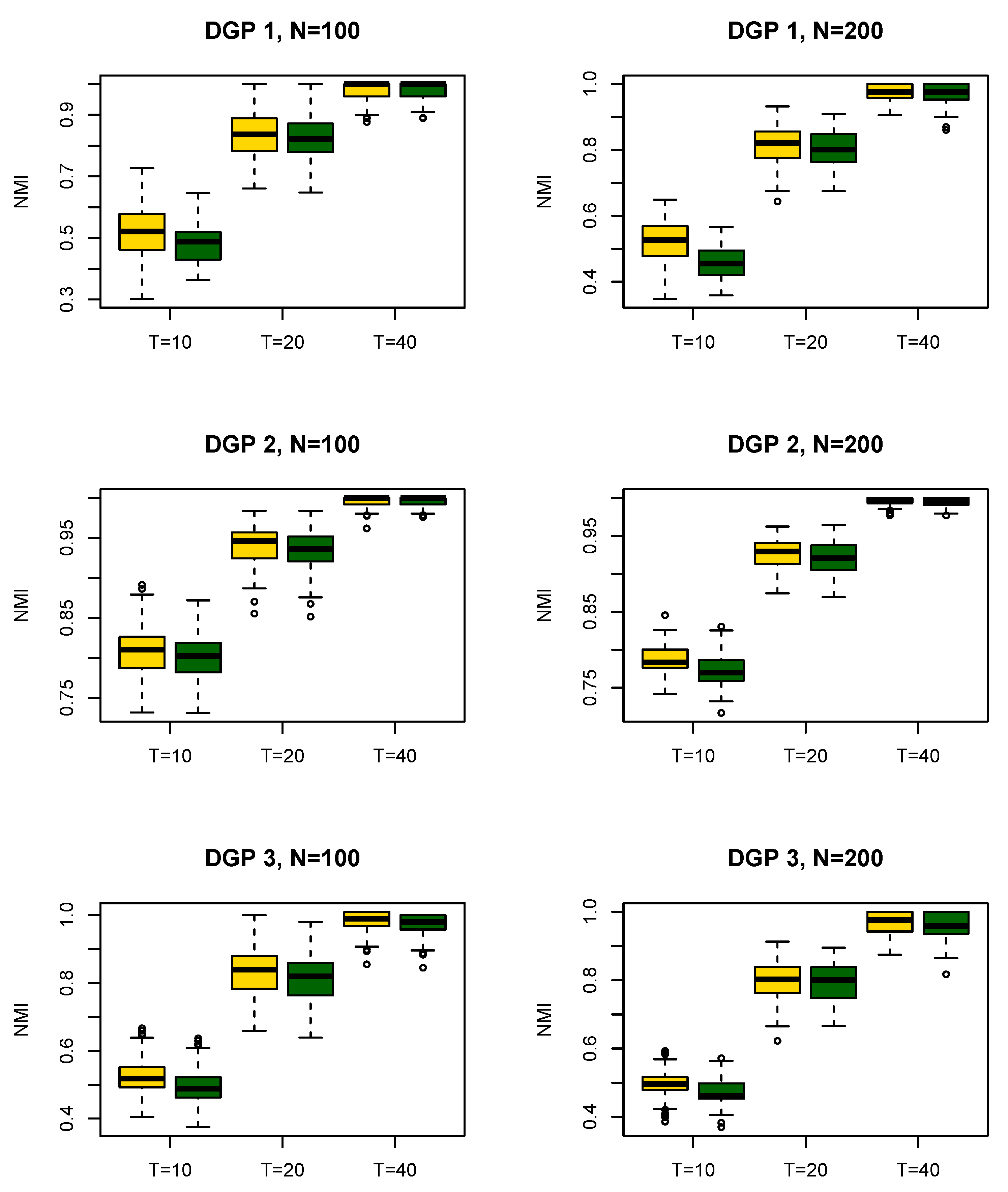
4.2. Simulation Results

We present the frequency with which a specific number of groups is obtained across 300 replications for all DGPs. While the accurate determination of the number of groups is undoubtedly crucial, this metric alone does not provide insight into the degree of similarity between the estimated groups and the true groups. Following [6], we employ the normalized mutual information (NMI) measure to assess the similarity between the estimated group structure $\widehat{\mathcal{G}}$ and the true group structure ${\mathcal{G}}^0$. Specifically, for two sets of disjoint clusters $\mathcal{A}=\{A_1,A_2,\cdots \}$ and $\mathcal{B}=\{B_1,B_2,\cdots \}$ on the same set $\{1,\cdots ,N\}$, the NMI is defined as

$$\mathrm{NMI}(\mathcal{A},\mathcal{B})={\displaystyle \frac{I(\mathcal{A};\mathcal{B})}{\left[H\right(\mathcal{A})+H(\mathcal{B}\left)\right]/2}}$$

where

$$I(\mathcal{A};\mathcal{B})=\sum _{i,j}\left(\right|A_i\cap B_j|/N)log\left({\displaystyle \frac{N|A_i\cap B_j|}{|A_i|·|B_j|}}\right)\mathrm{and}H\left(\mathcal{A}\right)=-\sum _i{\displaystyle \frac{|A_i|}{N}}log\left({\displaystyle \frac{|A_i|}{N}}\right),$$

where $\left|A\right|$ denotes the cardinality of set A. Obviously when two groupings are exactly the same, i.e., $\mathcal{A}=\mathcal{B}$, we have $I(\mathcal{A};\mathcal{B})=H\left(\mathcal{A}\right)=H\left(\mathcal{B}\right)$, and $\mathrm{NMI}(\mathcal{A},\mathcal{B})=1$. In general, the NMI measure takes values on $[0,1]$, and larger NMI implies the two group structures are closer. To measure the estimation accuracy for slope parameters, we use the average model error, which is defined as ${\displaystyle \frac{1}{N}}{(\widehat{\mathit{\beta }}-{\mathit{\beta }}^0)}^{\mathrm{T}}(\widehat{\mathit{\beta }}-{\mathit{\beta }}^0)$.

Figure 1 reports the classification results across DGPs 1–3 for difference combinations of N and T. The yellow and green boxes represent the detection results with and without prior constraints, respectively. It shows the NMI between the estimated group structure $\widehat{\mathcal{G}}$ and the true group structure ${\mathcal{G}}^0$, and suggests that, as N or T increase, the NMI increases rapidly for both methods. More importantly, our method exhibits higher NMI values across all DGPs, which implies that incorporating prior information can substantially improve the classification performance. This phenomenon is particularly pronounced when T is small. We display the average model estimation error in Figure 2. As expected, the average model estimation error decreases as N or T increase. It is obvious that the proposed parameter estimators has smaller estimation biases, since some prior constraint information can help us to gain the extra efficiency of homogeneity detection.

Next, give the number of groups, we focus on the point estimation of the post-Lasso estimator. To save space, we report only the simulation results of the first group-specific parameter of all DGPs in

Table 3. The parameter estimation results of ${\alpha }_{11}$ for DGPs 1-3 based on $N=200$.

DGP		No-Prior [5]			Prior			Oracle
		$\mathit{T}=\mathbf{10}$	$\mathit{T}=\mathbf{20}$	$\mathit{T}=\mathbf{40}$	$\mathit{T}=\mathbf{10}$	$\mathit{T}=\mathbf{20}$	$\mathit{T}=\mathbf{40}$	$\mathit{T}=\mathbf{10}$	$\mathit{T}=\mathbf{20}$	$\mathit{T}=\mathbf{40}$
1	Bias	−0.025	−0.008	−0.002	−0.007	−0.004	−0.003	0.010	−0.001	−0.002
	SD	0.088	0.042	0.029	0.084	0.041	0.029	0.054	0.037	0.029
	ESE	0.060	0.041	0.029	0.062	0.042	0.029	0.058	0.041	0.029
	ECP	0.830	0.920	0.970	0.850	0.950	0.960	0.980	0.960	0.970
2	Bias	−0.011	−0.015	−0.001	0.008	−0.004	−0.001	−0.004	−0.007	0.000
	SD	0.086	0.040	0.027	0.089	0.042	0.027	0.062	0.040	0.027
	ESE	0.060	0.042	0.029	0.061	0.042	0.029	0.058	0.041	0.029
	ECP	0.780	0.980	0.960	0.830	0.950	0.960	0.940	0.980	0.970
3	Bias	0.005	0.003	0.003	0.018	0.005	0.004	0.005	0.004	0.003
	SD	0.078	0.042	0.031	0.077	0.043	0.032	0.060	0.042	0.031
	ESE	0.066	0.043	0.029	0.065	0.043	0.029	0.058	0.041	0.029
	ECP	0.910	0.970	0.930	0.920	0.960	0.920	0.940	0.950	0.930

Bias is empirical bias; SD is the Monte Carlo standard deviation; ESE is the estimated standard error and ECP is the empirical coverage probability of 95% Wald confidence interval.

, based on $N=200$ individuals. The oracle estimators, which assume that the latent group is known, are also included for comparison. As shown in the Table, the biases of the three types of estimators become negligible as T increases, indicating that all the estimators are consistent. Additionally, the standard deviations (SD) are close to their corresponding estimated standard errors (ESE), and the empirical coverage probabilities (ECP) converge to the nominal level of 95%. This validates the asymptotic normality properties of the proposed estimator, as demonstrated in Theorem 1. The no-prior estimators yield relatively smaller ECP and larger biases compared to the other two types of estimators, especially when T is small. Undoubtedly, the oracle estimators perform reasonably well, and our method produce results closer to those of the oracle estimators. In summary, incorporating prior information significantly improves the finite sample performance in terms of estimation efficiency, particularly when the time span is small.

5. Empirical Analysis

With the deepening of China’s reform and opening up, the country has undergone profound changes over the past few decades, becoming the second-largest economic entity and the second-largest power consumer in the world. It is well known that electricity plays a crucial role in both human activity and industrial production, including sectors such as communication and engineering. Thus, electricity serves as a solid foundation for economic development. Consequently, many researchers have focused on the relationship between electricity consumption and economic growth. For example, ref. [33] found that real GDP and electricity consumption in China are cointegrated using data from 1971 to 2004. Additionally, ref. [34] investigated the relationship between electricity consumption and economic growth through a panel data analysis. China’s vast territory encompasses 34 provinces, municipalities, and autonomous regions, creating a significant domestic market. This paper primarily focuses on the homogeneous effect of electricity consumption on GDP across these provinces.

GDP is the most closely monitored statistical index in macroeconomics and serves as an important measure of economic development. At the beginning of each year, the Chinese government releases the provincial GDP data for the previous year. The electricity consumption data used in this study are derived from the Li Keqiang Index (https://en.wikipedia.org/wiki/Li_Keqiang_index#) (accessed on 1 February 2025), which has been cited by The Economist as a reliable measure of China’s economy. This index incorporates three indicators electricity consumption, railway cargo volume, and bank lending that reflect the operation of China’s economy more accurately. Due to significant data gaps and challenges in data collection, the Tibet Autonomous Region, Hong Kong, Macao, and Taiwan are excluded from this analysis. Therefore, the study includes a total of 30 provinces, with observations spanning from 2001 to 2019, resulting in $N=30$ and $T=19$. All data utilized in this study are sourced from the China Statistical Yearbook Database, available at https://www.stats.gov.cn/sj/ndsj (accessed on 1 February 2025).

We first examine the existence of a homogeneous effect across provinces using a residual-based bootstrapping procedure. The detailed algorithm can be found in the Appendix. The resulting p-value is very close to zero, indicating the statistical significance of the homogeneous effect. Moreover, numerous empirical analyses suggest a positive relationship between GDP and electricity consumption. Therefore, we assume that the coefficients for all provinces are positive as prior information. To investigate this hidden homogeneity, we consider the following linear fixed effects model with a latent group structure:

$$y_{it}={\mu }_i+x_{it}{\beta }_i+{ϵ}_{it},i=1,\cdots ,N;t=1,\cdots ,T,s.t.{\beta }_i>0,$$

where $y_{it}$ is the logarithm of GDP for the ith province at the tth year, $x_{it}$ represents electricity consumption, ${\mu }_i$ characterizes the fixed effect, and ${ϵ}_{it}$ is the error term. The prior information here includes a inequality constraint for parameters ${\beta }_i$’s, i.e., $\mathcal{C}=\{{\beta }_i>0,i=1,\cdots ,N\}$.

Table 4. Classification results among 30 provinces in China.

With Prior Information		Without Prior Information
Group 1	Group 2	Group 1	Group 2	Group 3	Group 4	Group 5
$1.1692$	$3.4770$	$0.6935$	$0.8715$	0.9837	1.0879	3.4351
Anhui	Beijing	Guangdong	Shandong	Zhejiang	Anhui	Beijing
Fujian	Gansu	Jiangsu			Fujian	Gansu
Guangdong	Guizhou				Guangxi	Guizhou
Guangxi	Heilongjiang				Hainan	Heilongjiang
Hainan	Jilin				Hebei	Jilin
Hebei	Jiangxi				Henan	Jiangxi
Henan	Ningxia				Hubei	Ningxia
Hubei	Qinghai				Hunan	Qinghai
Hunan	Shannxi				Liaoning	Shannxi
Jiangsu	Tianjin				Inner Mongolia	Tianjin
Liaoning	Chongqing				Shanxi	Chongqing
Inner Mongolia					Shanghai
Shandong					Sichuan
Shanxi					Xinjiang
Shanghai					Yunan
Sichuan
Xinjiang
Yunnan
Zhejiang

presents the classification results using two different approaches: the proposed estimator incorporating the inequality constraint $\mathcal{C}$ and the PGFAL estimator proposed by [15] that does not account for the prior constraint. Using our proposed ADMM algorithm described in Algorithm 1, the provinces are divided into two groups. As shown by the Table, Group 1 includes provinces such as Anhui, Fujian, Guangdong, Guangxi, Hainan, Hebei, Henan, Hubei, Hunan, Jiangsu, Liaoning, Inner Mongolia, Shandong, Shanxi, Shanghai, Sichuan, Xinjiang, Yunnan, and Zhejiang, with an estimated coefficient of 1.1692. Group 2 comprises Beijing, Gansu, Guizhou, Heilongjiang, Jilin, Jiangxi, Ningxia, Qinghai, Shaanxi, Tianjin, and Chongqing, with a significantly higher coefficient of 3.4770.

Group 1 consists largely of provinces from the Eastern and Central regions, characterized by advanced industrialization, technological innovation, and a strong emphasis on services and capital investment. In these regions, the direct relationship between electricity consumption and economic growth is weaker, as economic growth is increasingly driven by non-energy-intensive sectors. While electricity consumption remains significant, its marginal impact on GDP growth is reduced due to energy efficiency improvements and shifts toward high-value-added industries. Group 2, primarily consisting of provinces from the Western and Northeastern regions, shows a stronger dependency of economic growth on electricity consumption. These regions are still in the process of industrialization, infrastructure development, and urbanization, making electricity consumption a crucial driver of economic growth. Beijing, Tianjin, and Chongqing are notable inclusions in Group 2 despite being considered economically advanced. This classification can be explained by the ongoing infrastructure expansion and high-tech investments in these cities, which require substantial energy inputs. Beijing and Tianjin, while economically developed, are still heavily investing in energy-demanding sectors such as smart technologies, urban infrastructure, and research and development. Chongqing, traditionally an industrial city, continues to undergo substantial industrialization and urban expansion, further increasing its reliance on electricity consumption for growth. This observation is consistent with the findings of [35,36], who reported that in Western regions, energy consumption has a significant causal relationship with economic growth, while in Eastern and Central regions, this relationship is less pronounced. This pattern highlights the varying roles of electricity consumption in different stages of industrialization across China provinces, where more industrialized areas show diminishing returns from energy use, and less industrialized areas remain heavily reliant on electricity to drive economic growth.

However, if we do not consider the prior information, the provinces are classified into five groups, which consist of 2, 1, 1, 15 and 11 province(s) with the corresponding group-specific coefficients 0.6935, 0.8715, 0.9837, 1.0879 and 3.4351, respectively. This suggest that imposing the prior information helps to prevent overly divergent groupings, thus leading to more stable classifications. We also calculate the mean squared prediction errors (MSPE) of these two methods. Specifically, the observations of all individuals in the first 12 years are used as the training set, while the observations in the subsequent 7 years serves as the validation set. Based on the identified latent structures, we calculate the MSPE as

$$\mathrm{MSPE}={\displaystyle \frac{1}{N|{\mathcal{T}}_{\mathrm{val}}|}}\sum _{i=1}^N\sum _{t\in {\mathcal{T}}_{\mathrm{val}}}{({\widehat{y}}_{it}-y_{it})}^2,$$

where ${\mathcal{T}}_{\mathrm{val}}=\{13,\cdots ,19\}$, $y_{it}$ is the true observation and ${\widehat{y}}_{it}$ is the prediction value. As a result, the MSPE of our estimator is 0.8396, while the MSPE without prior information is 3.9443, much larger than our method. The reduced prediction error illustrates that incorporating prior constraint information can improve the predictive performance in latent structures identification for panel models.

6. Discussion

Identifying the latent groups structures in panel data analysis has recently attracted significant research interest. In this paper, we explore a pairwise fusion approach incorporating prior constraint information to identify the group pattern, and design an efficient ADMM algorithm to solve the optimization problem. Simulation studies and a real data application show that the proposed estimators outperform the existing approaches in terms of both detection accuracy and predictive performance. Our work still has its limitations; for example, how to obtain the prior constraint information in practical data analysis. Besides, our asymptotic results are built on the condition that the prior information is correctly specified; however, it remains to be explored when the prior information is misspecified.

There are some interesting issues that warrant further research. First, we only consider the commonly-used linear panel model with individual fixed effects. It is possible to adapt our proposed estimation framework to other panel models with latent group structures, such as the panel models with endogenous regressors [5] or the nonlinear panel models [19]. The specific objective function and estimation routine need to be re-examined. Second, the selection consistency property in Theorem 2 assumes that the true number of groups $K^0$ is fixed. It is appealing to consider a general framework that allows $K^0$ increases with the sample size. However, it may bring additional technical difficulties. Third, it is reasonable to allow for the presence of cross-section dependence in the current models. For such case, utilizing the factor structure [37] or interactive fixed effects [38] is potentially feasible but would require specific efforts. We leave these issues as our future research topics.

References

1. Hsiao, C. Analysis of Panel Data; Number 54; Cambridge University Press: Cambridge, UK, 2014. [Google Scholar]
2. Bonhomme, S.; Manresa, E. Grouped patterns of heterogeneity in panel data. Econometrica 2015, 83, 1147–1184. [Google Scholar] [CrossRef]
3. Su, L.; Chen, Q. Testing homogeneity in panel data models with interactive fixed effects. Econom. Theory 2013, 29, 1079–1135. [Google Scholar] [CrossRef]
4. Phillips, P.C.; Sul, D. Transition modeling and econometric convergence tests. Econometrica 2007, 75, 1771–1855. [Google Scholar] [CrossRef]
5. Su, L.; Shi, Z.; Phillips, P.C. Identifying latent structures in panel data. Econometrica 2016, 84, 2215–2264. [Google Scholar] [CrossRef]
6. Ke, Z.T.; Fan, J.; Wu, Y. Homogeneity pursuit. J. Am. Stat. Assoc. 2015, 110, 175–194. [Google Scholar] [CrossRef]
7. Xiao, D.; Ke, Y.; Li, R. Homogeneity structure learning in large-scale panel data with heavy-tailed errors. J. Mach. Learn. Res. 2021, 22, 1–42. [Google Scholar]
8. Zhang, Y.; Wang, H.J.; Zhu, Z. Quantile-regression-based clustering for panel data. J. Econom. 2019, 213, 54–67. [Google Scholar] [CrossRef]
9. Fan, J.; Li, R. Variable selection via nonconcave penalized likelihood and its oracle properties. J. Am. Stat. Assoc. 2001, 96, 1348–1360. [Google Scholar] [CrossRef]
10. Tibshirani, R. Regression shrinkage and selection via the lasso. J. R. Stat. Soc. Ser. Stat. Methodol. 1996, 58, 267–288. [Google Scholar] [CrossRef]
11. Huang, W.; Jin, S.; Su, L. Identifying latent grouped patterns in cointegrated panels. Econom. Theory 2020, 36, 410–456. [Google Scholar] [CrossRef]
12. Huang, W.; Su, L.; Zhuang, Y. Detecting unobserved heterogeneity in efficient prices via classifier-lasso. J. Bus. Econ. Stat. 2023, 41, 509–522. [Google Scholar] [CrossRef]
13. Su, L.; Ju, G. Identifying latent grouped patterns in panel data models with interactive fixed effects. J. Econom. 2018, 206, 554–573. [Google Scholar] [CrossRef]
14. Su, L.; Wang, X.; Jin, S. Sieve estimation of time-varying panel data models with latent structures. J. Bus. Econ. Stat. 2019, 37, 334–349. [Google Scholar] [CrossRef]
15. Mehrabani, A. Estimation and identification of latent group structures in panel data. J. Econom. 2023, 235, 1464–1482. [Google Scholar] [CrossRef]
16. Ando, T.; Bai, J. Panel data models with grouped factor structure under unknown group membership. J. Appl. Econom. 2016, 31, 163–191. [Google Scholar] [CrossRef]
17. Liu, R.; Shang, Z.; Zhang, Y.; Zhou, Q. Identification and estimation in panel models with overspecified number of groups. J. Econom. 2020, 215, 574–590. [Google Scholar] [CrossRef]
18. Bai, J. Estimating multiple breaks one at a time. Econom. Theory 1997, 13, 315–352. [Google Scholar] [CrossRef]
19. Wang, W.; Su, L. Identifying latent group structures in nonlinear panels. J. Econom. 2021, 220, 272–295. [Google Scholar] [CrossRef]
20. Su, L.; Wang, W.; Xu, X. Identifying latent group structures in spatial dynamic panels. J. Econom. 2023, 235, 1955–1980. [Google Scholar] [CrossRef]
21. Wang, Y.; Phillips, P.C.; Su, L. Panel data models with time-varying latent group structures. J. Econom. 2024, 240, 105685. [Google Scholar] [CrossRef]
22. Beer, J.C.; Aizenstein, H.J.; Anderson, S.J.; Krafty, R.T. Incorporating prior information with fused sparse group lasso: Application to prediction of clinical measures from neuroimages. Biometrics 2019, 75, 1299–1309. [Google Scholar] [CrossRef] [PubMed]
23. Li, Y.; Jin, B. Pairwise fusion approach incorporating prior constraint information. Commun. Math. Stat. 2020, 8, 47–62. [Google Scholar] [CrossRef]
24. Li, F.; Sang, H. Spatial homogeneity pursuit of regression coefficients for large datasets. J. Am. Stat. Assoc. 2019, 114, 1050–1062. [Google Scholar] [CrossRef]
25. Zhang, X.; Liu, J.; Zhu, Z. Learning coefficient heterogeneity over networks: A distributed spanning-tree-based fused-lasso regression. J. Am. Stat. Assoc. 2024, 119, 485–497. [Google Scholar] [CrossRef]
26. Wang, W.; Phillips, P.C.; Su, L. Homogeneity pursuit in panel data models: Theory and application. J. Appl. Econom. 2018, 33, 797–815. [Google Scholar] [CrossRef]
27. Boyd, S.; Parikh, N.; Chu, E. Distributed Optimization and Statistical Learning via the Alternating Direction Method of Multipliers; Now Publishers Inc.: Delft, The Netherlands, 2011. [Google Scholar]
28. Ke, Y.; Li, J.; Zhang, W. Structure identification in panel data analysis. Ann. Stat. 2016, 44, 1193–1233. [Google Scholar] [CrossRef]
29. Ma, S.; Huang, J. A concave pairwise fusion approach to subgroup analysis. J. Am. Stat. Assoc. 2017, 112, 410–423. [Google Scholar] [CrossRef]
30. Jeon, J.-J.; Kwon, S.; Choi, H. Homogeneity detection for the high-dimensional generalized linear model. Comput. Stat. Data Anal. 2017, 114, 61–74. [Google Scholar] [CrossRef]
31. Zhang, C.-H. Nearly unbiased variable selection under minimax concave penalty. Ann. Stat. 2010, 38, 894–942. [Google Scholar] [CrossRef]
32. Belloni, A.; Chernozhukov, V. Least squares after model selection in high-dimensional sparse models. Bernoulli 2013, 19, 521–547. [Google Scholar] [CrossRef]
33. Shiu, A.; Lam, P.-L. Electricity consumption and economic growth in china. Energy Policy 2004, 32, 47–54. [Google Scholar] [CrossRef]
34. Xu, S.-C.; He, Z.-X.; Long, R.-Y. Factors that influence carbon emissions due to energy consumption in china: Decomposition analysis using lmdi. Appl. Energy 2014, 127, 182–193. [Google Scholar] [CrossRef]
35. Akkemik, K.A.; Göksal, K.; Li, J. Energy consumption and income in chinese provinces: Heterogeneous panel causality analysis. Appl. Energy 2012, 99, 445–454. [Google Scholar] [CrossRef]
36. Wang, N.; Fu, X.; Wang, S. Economic growth, electricity consumption, and urbanization in china: A tri-variate investigation using panel data modeling from a regional disparity perspective. J. Clean. Prod. 2021, 318, 128529. [Google Scholar] [CrossRef]
37. Pesaran, M.H. Estimation and inference in large heterogeneous panels with a multifactor error structure. Econometrica 2006, 74, 967–1012. [Google Scholar] [CrossRef]
38. Miao, K.; Li, K.; Su, L. Panel threshold models with interactive fixed effects. J. Econom. 2020, 219, 137–170. [Google Scholar] [CrossRef]
39. Tseng, P. Convergence of a block coordinate descent method for nondifferentiable minimization. J. Optim. Theory Appl. 2001, 109, 475–494. [Google Scholar] [CrossRef]
Figure 1. The normalized mutual information across different N and T for DGPs 1–3.
Mathematics 13 01505 g001
Figure 2. The average model estimation errors across different N and T for DGPs 1–3.
Mathematics 13 01505 g002