Article

Dual-Resource Scheduling with Improved Forensic-Based Investigation Algorithm in Smart Manufacturing

1
School of Information Engineering, Wuhan University of Technology, Wuhan 430070, China
2
School of Information Engineering, Hubei University of Economics, Wuhan 430205, China
3
Hubei Key Laboratory of Digital Finance Innovation, Hubei University of Economics, Wuhan 430205, China
*
Author to whom correspondence should be addressed.
Mathematics 2025, 13(9), 1432; https://doi.org/10.3390/math13091432
Submission received: 29 March 2025 / Revised: 23 April 2025 / Accepted: 25 April 2025 / Published: 27 April 2025

Abstract

:
With increasing labor costs and rapidly dynamic changes in the market demand, as well as realizing the refined management of production, more and more attention is being given to considering workers, not just machines, in the process of flexible job shop scheduling. Hence, a new dual-resource flexible job shop scheduling problem (DRFJSP) is put forward in this paper, considering workers with flexible working time arrangements and machines with versatile functions in scheduling production, as well as a multi-objective mathematical model for formalizing the DRFJSP and tackling the complexity of scheduling in human-centric manufacturing environments. In addition, a two-stage approach based on a forensic-based investigation (TSFBI) is proposed to solve the problem. In the first stage, an improved multi-objective FBI algorithm is used to obtain the Pareto front solutions of this model, in which a hybrid real and integer encoding–decoding method is used for exploring the solution space and a fast non-dominated sorting method for improving efficiency. In the second stage, a multi-criteria decision analysis method based on an analytic hierarchy process (AHP) is used to select the optimal solution from the Pareto front solutions. Finally, experiments validated the TSFBI algorithm, showing its potential for smart manufacturing.

1. Introduction

Industry 5.0 has revolutionized traditional manufacturing by incorporating advanced information and communication technologies, including cyber–physical systems (CPSs), big data analytics, machine learning, and the Internet of Things (IoT). This change has led intelligent manufacturing into a new era dominated by digitalization and services. The emergence of these technologies not only enables the manufacturing industry to better meet the increasingly personalized demands of the market but also enhances its overall competitiveness. In this dynamic context, research aimed at optimizing manufacturing processes, especially in areas such as production scheduling, becomes crucial.
Efficient production scheduling is extremely important to optimize the cost-effectiveness and productivity of manufacturing systems, especially in flexible job shops. Over the years, the flexible job shop scheduling problem (FJSP) has been extensively studied [1]. However, historically, FJSP research has focused on optimizing machine resources but neglected labor resource management. In the modern manufacturing industry, labor resource management has gradually become a key factor in determining the performance of the whole system.
With the development of Industry 5.0, the importance of human–machine integration has become increasingly prominent [2]. This trend has mainly been driven by two factors: escalating labor costs and the need for more adaptive and resilient production systems [3]. Dual-Resource Constraint (DRC) systems [4], which combine human and machine resources, have received extensive attention in the field of flexible job shop scheduling. These systems leverage multi-skilled workers and flexible work schedules to increase resource utilization, improve worker satisfaction, and increase the overall productivity. Multiple studies [5,6] have investigated the flexible job shop problem (FJSP) involving multi-skilled workers and their impact on the processing time. Nevertheless, workers acquire their multiple skills through training, which incurs substantial training costs [7]. Consequently, shops tend to employ a higher proportion of single-skilled workers or a limited number of skilled workers.
Moreover, numerous studies have demonstrated that flexible working time arrangements play a pivotal role in promoting a work–life balance among employees and enhancing the overall company’s productivity [8]. The production tasks change from batch to batch in the shop, which usually leads to changes in the number of people responsible for production. Nevertheless, a standard work system in workshops is to assign a fixed number of workers to each batch of tasks, and they work for a continuous and fixed period, such as from 9 a.m. to 5 p.m. [9]. Although this method can effectively use the available human resources, redundancy can occur when the tasks are too few. For example, a job requires only four people to complete production. Still, with a fixed arrangement of five people, the work efficiency will be the same, and the personnel cost will significantly increase. Moreover, in the case of there being too many tasks, measures such as extra overtime are required due to insufficient staff. In such cases, flexible working time arrangements present a potential solution to optimize labor deployment, reduce personnel costs, and enhance operational efficiency.
Hence, a DRFJSP considering workers with flexible working time arrangements and machines with versatile functions is presented. This approach aligns with the Industry 5.0 paradigm by emphasizing adaptability, resilience, and the integration of human and machine resources. To address the computational complexity of dual-resource scheduling in smart manufacturing, this study adopted the forensic-based investigation (FBI) algorithm due to a strategic rationale: the interpopulation cooperation mechanism inherent in the FBI algorithm uniquely mirrors the dynamic coupling of machines and workers in DRC systems. Unlike traditional genetic algorithms that often struggle with premature convergence, an FBI’s two-stage investigation-tracking mechanism systematically balances exploration and exploitation at the multi-objective Pareto frontier. The remaining parts of this paper are organized as follows. A literature review is presented in Section 2. In Section 3 the scheduling problem and formal description are elaborated. In Section 4, the two-stage FBI-based algorithm is introduced. The case study and analyses are described in Section 5. Finally, the conclusions and future perspectives are stated in Section 6.

2. Literature Review

Industry 5.0 highlights a human-centric approach that prioritizes sustainable development and production flexibility [10]. In manufacturing, production systems must both serve and rely on human resources [11]. This paper investigates two areas: (1) the impact of working hours on workers and (2) the influence of human-inspired decision-making on algorithmic scheduling in production systems. In highly automated manufacturing environments, human intervention remains essential for tasks that cannot or should not be automated due to technical, socioeconomic, or ethical reasons. The goal of automation is not to replace workers, but to de-skill tasks so that workers can use their expertise, intelligent tools, and assistive systems to focus on decision-making and control. Therefore, human resources are the core of the production process, and their management and utilization require in-depth research [12].
Production scheduling plays an essential role in the implementation of production. It can organically combine various elements (human resources, machines, materials, rules, and the environment) of the production process [13]. Within this, dual-resource scheduling, especially a dual-resource scheduling problem that considers both worker resources and machine resources, has been widely studied by researchers. Further research has explored various facets of the DRFJSP, often extending the problem scope or constraints. For instance, Gong [14] introduced a double flexible job shop problem (DFJSP), optimizing the processing time, green production, and human factors using a hybrid genetic algorithm. Yu [15] studied distributed assembly hybrid flow shops with dual-resource constraints (DAHFSSP-DRC), minimizing the total tardiness using a knowledge-based iterated greedy algorithm. Mlekusch [16] considered a dual-resource-constrained re-entrant flexible flow shop, common in screen printing, minimizing the makespan using constraint programming and a hybrid genetic algorithm. Renna [17] applied game theory (Gale–Shapley model) for worker assignment in DRC job shops, showing its benefits, especially with varying worker efficiencies. Li [18] specifically focused on worker shift arrangements in the FJSP, using a two-stage algorithm to minimize overdue days while managing shifts. Xiao [19] tackled stochastic processing times in the DR-SJSSP using a robust scheduling approach and a two-stage assignment strategy solved using MO-HEDA. Li [20] addressed sustainability (makespan, energy, ergonomics) in the SFJSPCDR using a survival duration-guided NSGA-III. Wei [21] proposed an inverse scheduling approach for the RCFJISP to handle uncertainties by adjusting machine, worker, and process parameters using an improved memetic algorithm. Berti [22] incorporated aging workforce effects and fatigue into DRC job shop scheduling, evaluating the impact of rest allowances. Seifi [23] formulated MILP models for simultaneous machine and worker assignment in shift-based potash mining operations. Santos [24] integrated machine scheduling (batch job shop) and personnel allocation in large-scale facilities using a rolling horizon framework. While these studies have significantly advanced the understanding of the DRFJSP, exploring areas like double flexibility [14], assembly [15], re-entrance [16], worker assignment strategies [17,19,20], shift scheduling [18,23], sustainability [20], uncertainty/robustness [21], and worker characteristics like fatigue/aging [22], relatively few have specifically examined the impact of flexible working time arrangements, where workers operate within defined total hour limits rather than in fixed shifts or on simple multi-skilling assignments, on the scheduling performance and cost.
Flexible working time arrangements, which allow employees to manage their work hours outside the traditional “9 to 5” framework, have been shown to enhance employee motivation and productivity [25]. Baridula [26] highlighted their role in increasing employee retention in Nigerian manufacturing firms. Jarrahi [9] suggested that personal digital infrastructure facilitates the implementation of flexible working time systems. Despite these benefits, the impact of flexible working time arrangements on production scheduling remains underexplored. Therefore, this study distinguished itself by explicitly modeling and optimizing a DRFJSP variant that incorporates workers with flexible working time arrangements alongside versatile machines. Unlike studies focusing on fixed shifts or multi-skilling costs, our work investigated the potential cost and efficiency benefits derived from allowing workers flexible start/end times within overall working hour constraints, addressing a gap in optimizing adaptable human resource deployment in modern manufacturing.
In recent years, Delgoshaei [27] systematically reviewed the evolution of dual-resource scheduling approaches, identifying a paradigm shift toward the hybrid metaheuristics incorporating human factors that are a key foundation for our work. For the dual-resource-constrained flexible job shop scheduling problem (DRFJSP), a variety of metaheuristic methods have been widely used to cope with its NP-hard nature and obtain high-quality solutions in finite time. Metaheuristics have become a research hotspot because of their advantages regarding response time requirements in actual production systems [28]. However, as the well-known No Free Lunch (NFL) theorem [29] indicates, no metaheuristic is the most suitable for all optimization problems. This has motivated researchers to modify existing algorithms or develop new ones to solve various optimization problems [30], such as the DRFJSP. Metaheuristics can be classified into evolution-based, population-based, human-based, physics-based, systems-based, and biology-based approaches [31]. Traditional evolutionary algorithms such as genetic algorithms (GAs) and particle swarm optimization (PSO) have been widely used, but they often suffer from parameter sensitivity. For example, Mlekusch [16] demonstrated the effectiveness of constraint programming combined with genetic algorithms for re-entrant flow shops, achieving a 12–18% better makespan than pure GA implementations. However, their hybrid approach requires complex parameter coordination between constraint propagation and evolutionary operators, increasing the implementation complexity. Similarly, Lu [32] developed a memetic algorithm hybridizing a local search with genetic operators for assembly sequence variations, reducing the energy consumption by 17% compared to PSO-based approaches. The PSO implementation by Zhang [33] also led to local convergence due to the improper setting of the speed factor. Liu’s [34] improved biological migration algorithm demonstrated that parameter reduction can reduce the number of iterations by 35%. Therefore, a heuristic algorithm with low parameter tuning is especially useful for resource-constrained production systems that require fast response times.
Recent work has also extended the objectives beyond makespan minimization. Akbar [35] applied a variant of NSGA to balance tardiness and labor productivity, revealing an inherent conflict between these objectives that informed our Pareto frontier analysis. Yu [15] found that incorporating a knowledge-guided greedy search into the distributed assembly problem reduced the computation time by 28% compared to the Chinese implementation while maintaining a similar solution quality, supporting our hybrid decoding strategy. However, neither study addressed the critical integration problem concerning flexible working time constraints. The FBI algorithm is an optimization algorithm based on human behavior [36], and its algorithm performance is relatively excellent, especially since it does not require any complex parameters that would seriously affect the algorithm’s performance. It has been applied to and shown excellent results in the solution of problems in various fields, such as solar cell model parameter optimization, pavement pothole identification [37], and project scheduling [38]. Despite this, the application of the FBI algorithm to solve flexible job shop scheduling problems such as the DRFJSP is still limited. On the one hand, the original FBI algorithm is mainly designed for continuous optimization problems, and on the other hand, its structure is only suitable for single-objective optimization tasks, which restricts its application in multi-constrained, discrete, and multi-objective environments.
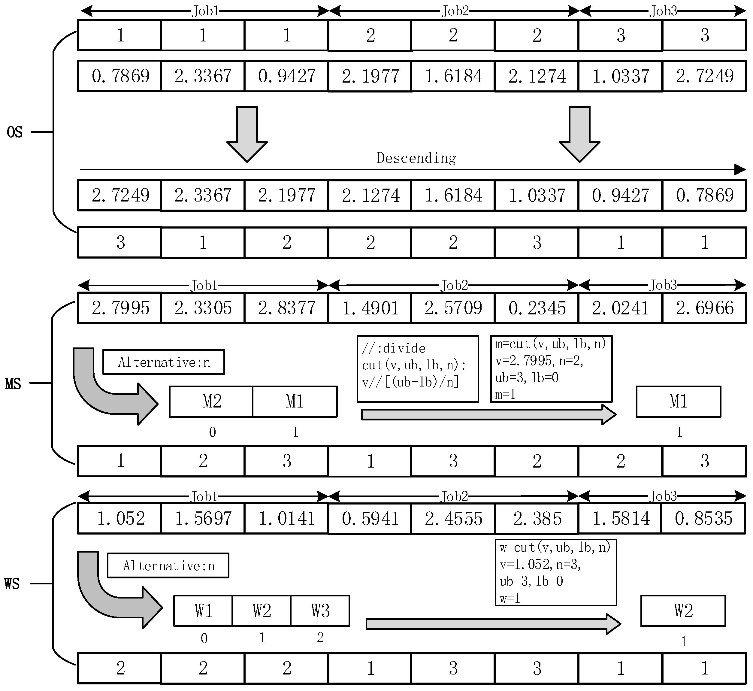
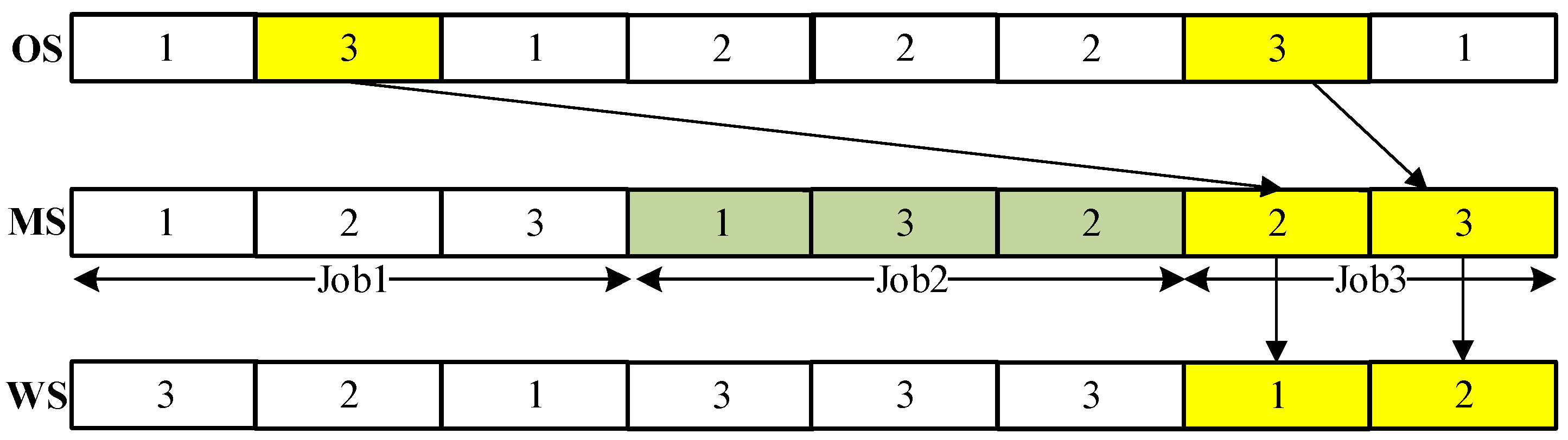
To address combinatorial optimization problems, continuous optimization algorithms often require modifications to their operators. For instance, crossover operations can replace addition operations to better suit discrete problem spaces [39,40]. However, more efficient approaches involve developing new discrete algorithms specifically tailored for combinatorial optimization, which increases the scaling cost and time. Some researchers [
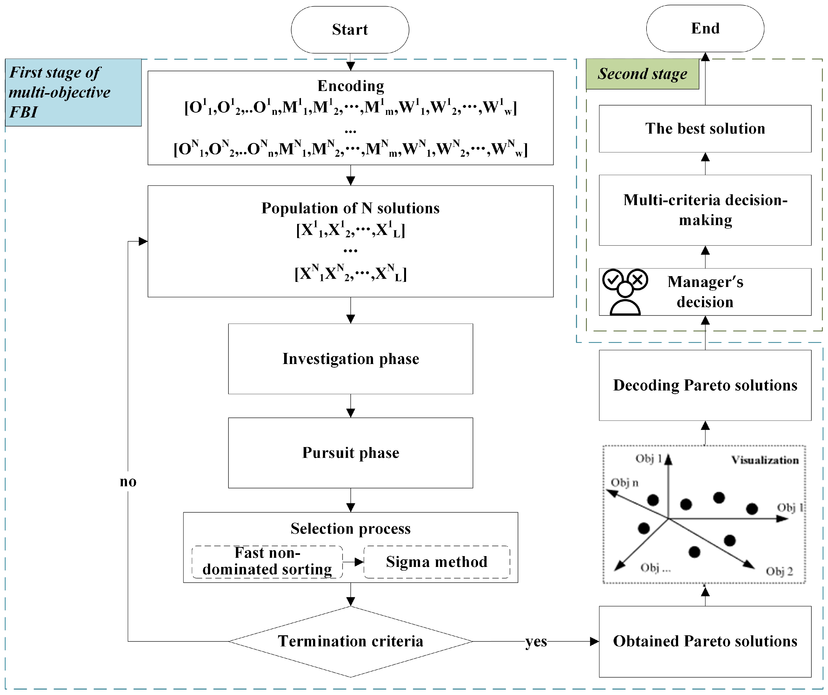
41] have identified the efficacy of the encoding and decoding methodology in transforming the design space into the problem space, and through the development of suitable coding and decoding techniques, it has become feasible to effectively enhance current algorithm versions, providing them with the capability to address combinatorial optimization problems. Hence, this paper presents a general hybrid coding and decoding method based on a technical characteristic of codecs so that the continuous optimization algorithm can quickly solve the combined optimization problem and reduce the cost and time consumption of developing a discrete version. Furthermore, since the dual-resource flexible job shop scheduling problem (DRFJSP) involves multiple objectives, the original forensic-based investigation (FBI) algorithm, designed for single-objective optimization, needed to be extended to handle multi-objective problems. Extensions of single-objective algorithms to multi-objective algorithms typically fall into four categories: dominance-based, decomposition-based, indicator-based, and hybrid selection mechanism-based approaches [42]. Among these, the dominance-based approach [42,43], which relies on the concept of Pareto dominance, is widely used and effective for finding a diverse set of trade-off solutions. Therefore, we employed a Pareto-based dominance method, specifically the fast non-dominated sorting approach, to extend the FBI algorithm for multi-objective optimization.
However, solving the DRFJSP using a multi-objective FBI algorithm yields a set of Pareto-optimal solutions, presenting a challenge for decision-makers in selecting the most satisfactory solution. To address this, multi-criteria decision-making (MCDM) methods were employed. The analytical hierarchy process (AHP) is a well-established MCDM method that effectively combines qualitative and quantitative analysis, making it suitable for scenarios with a limited number of objectives [44]. The AHP has been widely applied to multi-objective decision-making in combinatorial optimization problems [45,46], enabling managers to make informed decisions based on the production status and objectives. Due to its advantages of requiring less information and offering short decision times, this study applied AHP to the decision-making process for multi-objective scheduling problems in job shop environments.

3. Problem Description and Formulation

3.1. A Dual-Resource Flexible Job Shop Problem

The problem of the DRFJSP is described as follows. It contains a job set, J = {J1, J2, …, Jn}, a machine set, M = {M1, M2, …, Mm}, and a worker set, W = {W1, W2, …, Ww}. Each job, Ji, contains j process operations, and each operation must be completed in the proper order. O i j represents the jth process of the ith job. This process can only be undertaken using one machine within the selection of its optional machines, and only one worker can be selected to operate it. Each worker’s working hours are flexible, i.e., they can leave work once they have completed the standard working hours. These jobs are completed within a task period, and the number of workers is limited by the size of the workshop. The DRFJSP includes four sub-problems: machine allocation, the determination of the number of workers, worker selection, and operation sequencing. To clarify the proposed problem, we assume that the following rules limit the possible assignments of operations:
  • All jobs, workers, and machines are available at S 0 ;
  • The accumulated working hours of workers cannot exceed the upper bound of their working time;
  • The accumulated working hours of workers cannot be lower than the lower bound of their working time;
  • Overtime pay is α times the general salary;
  • Any operation within a job can only be undertaken after its preceding procedures have been completed;
  • The actual operating time of a worker is equivalent to the operating time of the equipment;
  • The standard completion time and standard cost of the procedure have been determined;
  • There is no sequential restriction on processes that are part of different jobs;
  • Each item of equipment can only complete one job at the same time;
  • One worker can only complete one job at the same time;
  • Once the process starts, it cannot be interrupted unless personnel change shifts and the shift change time is ignored.

3.2. Problem Formulation

A series of mathematical programming models concerning the FJSP have been presented in the literature so far. Demir [47] compared five different MILP models for the FJSP. They demonstrated that model M2 had the lowest computation time for almost all the optimally solved test problems, and they suggested using precedence variable-based models, especially model M2 for the FJSP. Although the proposed MILP model coped with a dual-resource FJSP, due to the number of binary and continuous variables and the structure of the model itself, it can be considered as having been partially derived from the above-mentioned Model 2. The MILP for the problem under investigation is as follows, and notations for the proposed DRFJSP are listed in Table 1.
A worker who works more than the standard hours is considered to be working overtime and requires additional overtime pay. If the overtime period is exceeded, the worker having had adequate rest cannot be guaranteed, and this situation is not allowed. When the working hours of workers violate the above constraints, this is unreasonable. Therefore, the total worker cost is the sum of the total cost of the standard working hours E 1 , the total cost of overtime E 2 , and the total base wage of the worker E 3 .
E 1 = i = 1 n j = 1 n i k M i j l W k ( C i j k l S i j k l ) × U i j k l
E 2 = m a x 0 , ( i = 1 n j = 1 n i k M i j l W k C i j k l S i j k l S T ) × U i j k l × β )
E 3 = l = 1 w B l
Based on the above-mentioned parameters, two objectives are shown as Equation (4). The first objective is to minimize the maximum completion time, which is one of the critical performance criteria for productivity. The second objective is to minimize the total labor costs. Equation (1) calculates the total labor cost incurred during standard working hours across all operations. It sums the product of the actual processing time ( C i j k l S i j k l ) and the corresponding unit time cost U i j k l for each operation, O i j , assigned to machine k and worker l, assuming the work is performed within the standard working hours limit.
Objectives:
min f 1 = C m a x min f 2 = E 1 + E 2 + E 3
subject to the following:
C m a x C i                       i J
C i k M i j l W k C i j k l                         i J ; j = 1 , , n i
S i j k l + C i j k l v i j k l × M                         i J ; j = 1 , , n i ; k M i j ; l W k
C i j k l S i j k l + T i j k l 1 v i j k l × M               i J ; j = 1 , , n i ; k M i j ; l W k
S i j k l C i j k l z i j k l , i j k l × M i , i J ; j , j = 1 , , n i ; k M i j ; l , l W k
S i j k l C i j k l ( 1 z i j k l , i j k l ) × M i , i J ; j , j = 1 , , n i ; k M i j ; l , l W k
k M i j l W k S i j k l k M i j l W k C i j 1 k l i J ; j = 2 , , n i ;
i = 1 n j = 1 n i k M i j ( C i j k l S i j k l ) U B T     l W k
i = 1 n j = 1 n i k M i j ( C i j k l S i j k l ) L B T     l W k
k M i j l W k v i j k l = 1               i J ; j = 1 , , n i
v i j k l ,   z i j k l , i j k l { 0 ; 1 } ; W k [ a , b ]
C i j k l , C i , S i j k l , S i j k l , C i j k l , C i j k l , C m a x R +
Constraint (5) ensures that the makespan corresponds to the maximum completion time among all jobs. Constraint (6) mandates that the completion time of each job must equal that of its last operation. Constraints (7) and (8) guarantee that the difference between the starting and completion times will be at least equal to the processing time on machine k. Constraints (9) and (10) establish that distinct jobs completed on the same machine simultaneously must adhere to a specific completion order. Constraint (11) stipulates that different process operations within the same job must follow a particular completion sequence. Constraints (12) and (13) impose upper and lower boundaries on the cumulative working time for each worker, while constraint (14) specifies that the same process operation may only be performed by one worker on the same machine. Constraints (15) and (16) define the decision variable range.

4. Two-Stage FBI-Based Algorithm

The proposed algorithm, called the TSFBI algorithm, for solving the DRFJSP consists of a Pareto optimization phase and a multi-criteria decision-making phase. In the Pareto optimization phase, a discrete multi-objective version of the FBI algorithm is used to obtain the Pareto solutions of the DRFJSP. On the other hand, the multi-criteria decision-making phase involves the selection of the best solution from the Pareto solutions. Figure 1 illustrates the main components of the TSFBI algorithm, which is executed according to the following steps.
  • Random initialization involves the construction of the scheduling solution set, which includes the population size (N), the number of objective functions (D), and the int part (IP) of the solution and maps the operation selection sequence, machine selection sequence, and worker selection sequence onto agent location vectors, X (the total length is three times the length of the process selection sequence), using a hybrid coding technique and records the mapping relationships. The detailed encoding process is described in Section 4.1.1.
  • The investigation phase involves setting up a team of agents, analyzing the suspect’s potential hiding places and determining the highest-probability suspicious locations, dividing the search area based on the suspicious locations, and setting up a pursuit team to enter the pursuit phase.
  • During the pursuit stage, the pursuit team follows the orders from the headquarters and moves closer to the suspicious spot, reporting all information related to the suspicious location; throughout the whole dispatch–discovery–approach process, the investigation and pursuit teams work closely together. For details on steps 2 and 3, see the original article [36] and Section 4.1.2.
  • After the completion of the pursuit, the existing solutions are sorted and selected to obtain the Pareto solutions in the following ways. First, the solutions are decoded to determine the scheduling goal; then, the solutions in the set are stratified by using fast non-dominated sorting to determine the domination relationship based on the scheduling goal; next, the quantitative fitness of the stratified solution set is calculated; and finally, a greedy selection strategy is used to perform population selection based on fitness in order to obtain the Pareto solutions. See Section 4.1.2 for the detailed process.
  • If the termination condition is satisfied, the loop is ended and the procedure progresses to step 6; if not, step 2 to step 4 are repeated.
  • The obtained Pareto solution set is decoded to obtain the Pareto solutions for scheduling and determine the target.
  • The analytical hierarchy process is used to evaluate and calculate the Pareto solutions, rank and select them based on the estimated values, and obtain the final scheduling solution.

4.1. Pareto Optimization Phase

The FBI algorithm is a novel optimization method used to determine global solutions for continuous linear functions with accuracy and low computational effort. It is inspired by police personnel, who carry out the investigation, location, and conviction of criminals, and it has two main phases, which are the investigation phase and the pursuit phase. While the investigator’s team carries out the investigation phase, the police agents’ team performs the pursuit phase. The original FBI algorithm is a single-objective optimization algorithm and is mainly used to solve continuous optimization problems. However, the proposed DRFJSP is a multi-objective combined optimization problem. Therefore, first, a hybrid coding approach was proposed to provide the algorithm with the ability to solve combinatorial optimization problems, and second, a multi-objective version of the FBI algorithm was constructed to obtain Pareto solutions.

4.1.1. A Hybrid Encoding and Decoding Method

The optimization operation mechanism in the original FBI uses real number solutions, and it is difficult to apply to combinatorial optimization problems such as the DRFJSP. Therefore, a hybrid encoding approach was proposed to derive a complete scheduling solution by constructing a mapping relationship between real number and integer solutions. The int part (IP) (also known as the chromosome sequence) includes the operation sequence (OS), machine sequence (MS), and worker sequence (WS), and the real part is the ordering and selection basis for these sequences, and I P = O S , M S , W S .
O S = O i c c = 1 , 2 , , N ; i = 1 , 2 , n . O i c denotes the number of the ith job of the cth individual, and its eth occurrence in the OS represents the eth operation of job i. M S = M i c c = 1 , 2 , , N ; i = 1 , 2 , n . M i c represents the machine number of the ith job completed by the cth individual. W S = W i c c = 1 , 2 , , N ; i = 1 , 2 , n   W i c represents the worker number assigned to the ith job of the cth individual. The real part is denoted by X , and   X = { X h c c = 1 , 2 , N ; h = 1 , 2 L ; f : I P X , and L is the length of the cth X . Figure 2 is a representative case of a concrete population where the int part of the OS is [1, 1, 1, 2, 2, 2, 3, 3] and the real part of the OS is [0.7869, 2.3367, 0.9427, 2.1977, 1.6184, 2.1274, 1.0337, 2.7249].
As the chromosome encoding sequence is a three-dimensional real number vector, three mapping relations exist for the encoding parts. Each mapping relation consists of a real part and an integer part, and each mapping relation has a real part and an integer part with different meanings due to the difference in the meaning of the sequences. In the OS, the real part represents the sorting rule, and the integer part represents the process number, i.e., the size of the real value determines the ordering of the elements in the integer part (descending order is used here). In the MS and WS, the real part represents the selection rule, and the integer part represents the number (we obtain the selected number by segmenting the selectable set and mapping the real numbers onto the corresponding interval segments, the algorithmic procedure for which is shown in Algorithm 1). The example shown in Figure 2 includes three jobs, the first and second with three operations and the third with two operations.
In the MS and WS, the real part represents the selection rule, and the integer part represents the selected machine or worker number, respectively. We obtain the selected number by segmenting the range of possible real values based on the number of available machines/workers for that operation and mapping the real number onto the corresponding interval segment (see Algorithm 1 for the mapping logic). For example, as shown in Figure 2 (which includes three jobs: Job 1 with three ops, Job 2 with three ops, Job 3 with two ops), the MS (machine sequence) row indicates the machine assigned to each operation, ordered according to the jobs (Job 1 ops, then Job 2 ops, then Job 3 ops). The green block [1, 3, 2] under ‘MS’ corresponds to the three operations of Job 2, meaning they are assigned to Machine 1, Machine 3, and Machine 2, respectively. The WS (worker sequence) row similarly indicates the worker assigned to each operation, following the same job order. The yellow block [1, 2] under ‘WS’ corresponds to the two operations of Job 3, signifying that Worker 1 operates the assigned machine (Machine 2, based on the MS) for operation O31, and Worker 2 operates the assigned machine (Machine 3, based on the MS) for operation O32.
Algorithm 1 Machine sequence relational mapping.
Input:The suspicious location vector (machine part) V, the max number of suspicious locations ub, the min number of suspicious locations lb, optional number of machines M
Output:The machine selection sequence MS
1. M S , i 0
2.for each  v V
3.          m M i
4.          t e m ( v l b i ) / / ( u b i l b i ) m ,   / /   m e a s   d i v i d e   u p w a r d
5.        MS M S m
The decoding process is referred to in Gong’s article [14], and the specific process is shown in the example in Figure 3, which indicates that the DRFJSP’s genetic code includes a three-layer genetic coding sequence for the OS, MS, and WS. The length of the process sequencing sequence is the sum of all operation processes.
The OS string dictates the sequence in which operations are considered for scheduling. Its length equals the total number of operations across all jobs. In Figure 3, the OS [1, 3, 1, 2, 2, 2, 3, 1] means that the first operation to be scheduled is the first operation of Job 1 (O11, indicated by the first ‘1’), the second is the first of Job 3 (O31), the third is the second of Job 1 (O12), and so on. The second ‘3’ in the OS refers to the second operation of Job 3 (O32).
The MS string provides the machine assignment for each operation. It is ordered job-wise, i.e., the first n 1 elements correspond to Job 1’s operations, the next n 1 to Job 2’s, etc. In Figure 3, for Job 1 (ops O11, O12, and O13), the MS segment [1, 2, 3] assigns the operations to Machines 1, 2, and 3, respectively. For Job 2 (ops O21, O22, and O23, green block), the MS [1, 3, 2] assigns them to Machines 1, 3, and 2. For Job 3 (ops O31 and O32, yellow block), the MS [2, 3] assigns them to Machines 2 and 3.
The WS string provides the worker assignments, also ordered job-wise, corresponding to the machine assignments from the MS. For Job 1, the WS [3, 2, 1] assigns Workers 3, 2, and 1 to operate Machines 1, 2, and 3, respectively, for O11, O12, and O13. For Job 2, the WS [3, 3, 3] assigns Worker 3 to all its operations. For Job 3 (yellow block), the WS [1, 2] assigns Worker 1 to operate Machine 2 for O31 and Worker 2 to operate Machine 3 for O32. By combining the processing order from the OS with the machine and worker assignments from the MS and WS, respecting job precedence constraints and the resource availability, a complete schedule with start and completion times can be constructed.

4.1.2. Multi-Objective FBI

The investigation phase comprises two steps. In the first step (A1), each candidate direction is calculated using Equation (17).
X h c ( A 1 ) = X h c ( A 1 ) + 2 r a n d 0.5 ( X h c ( A 1 ) ( X h c ( A 1 ) + X h c ( A 1 ) ) / 2 )
where X h c ( A 1 ) denotes the h th real value of the c th individual in phase A1, rand is a random number in the range [0,1], and h ,   h , and h are three indices.
In actual production, optimization problems often involve two or more conflicting objectives that need simultaneous consideration, such as minimizing the makespan and minimizing the personnel cost, as considered in this paper. For such multi-objective problems, there usually is not a single solution that optimizes all objectives concurrently. Instead, we seek a set of Pareto-optimal solutions. A solution is Pareto-optimal if no other feasible solution can improve one objective without degrading at least one other objective. When comparing two solutions, solution A dominates solution B if A is better than or equal to B regarding all objectives and strictly better regarding at least one objective. Solutions that are not dominated by any other solution in the feasible set are called non-dominated solutions. The set formed by all non-dominated solutions constitutes the Pareto-optimal set (or Pareto front in the objective space). The Pareto front visually represents the trade-offs inherent between the conflicting objectives; improving one objective typically requires sacrificing performance regarding another along this front. In a multi-objective FBI, the solutions are sorted based on the objective value of the solution using a low-time-complexity fast non-dominated sorting method to determine the dominance relationship of the solutions during each iteration so that the Pareto solutions can be found after multiple iterations. The fast non-dominated sorting algorithm is derived from NSGA-II [48]. In the NSGA-II algorithm, fast non-dominated sorting is used for population hierarchical sorting, and local crowding distances are used to make quantitative comparisons of individuals in the same hierarchy. This hierarchical comparison, which defaults to the first and last individuals in the sequence, is mandatory, and this default operation is also of a qualitative comparative nature. It is impossible to separate out the variability of each solution, and there is a risk of losing better individuals.
f i t n e s s i = d = 1 D f d i j = 1 N r a n k f d j + r a n k i 1 × 2 ,   i = 1 , 2 , n ; j = 1 , 2 , , N r a n k
This fitness calculation using the Sigma method [49] is designed to provide a quantitative measure for each solution after non-dominated sorting. It combines two components: (1) the non-domination rank ( r a n k i ), where solutions with better ranks (lower r a n k i value) receive significantly lower fitness values due to the ( r a n k i − 1) × 2 term, prioritizing convergence towards the Pareto front, and (2) a measure reflecting the solution’s normalized performance across all objectives relative to other solutions with the same rank (represented by the summation term as implemented in Algorithm 2). This second component allows for finer differentiation among solutions of the same non-dominated rank, aiming to quantitatively assess and preserve diversity better than methods relying solely on the crowding distance for intra-rank comparison.
The calculation function for the Sigma value (the smaller the value, the better the individual) is presented as Equation (18), where D is the total number of objectives, d is the current objective index, N r a n k is a number in the same r a n k i , r a n k i represents the current non-dominated ranking hierarchy of population i with a value greater than 1, and f d i represents the dth objective function of population i. The implementation of the Sigma method is shown in Algorithm 2.
Algorithm 2 Sigma method.
Input:The non-dominated set F, the rank set N r a n k , the number of objective D
Output:the fitness of population: f i t n e s s
1. f i t n e s s ,   β , N r a n k m a x m a x ( N r a n k )
2.for each  f l F
3.         S U M D , D I V D i ,
4.        for each  d D
5.                for each  f i f l
6.              S U M d   S U M d + f d i
7.        for each  d D
8.                for each  f i f l
9.                          D I V d i D I V d i + f d i S U M d
10.        for each  D I V d i D I V D i
11.              f i t n e s s i D I V d i + ( N r a n k f l 1 ) × 2
The second step (A2) involves the following modified probability calculation for multiple objective functions. The probability value of each individual is given by Equation (19). f i t n e s s w o r s t d and f i t n e s s b e s t d are the worst and the best fitness values of the d th objective function, respectively. f i t n e s s X c ( A 1 ) d is the objective function of individual X c ( A 1 ) . The P r o b   X c ( A 1 ) determines the probability that the value of X c ( A 1 ) is updated according to Equation (17).
P r o b   X c ( A 1 ) = d = 1 D ( f i t n e s s X c ( A 1 ) d f i t n e s s w o r s t d ) / ( f i t n e s s b e s t d f i t n e s s w o r s t d ) / d
The new suspected location of the suspect X h c ( A 2 ) is updated using Equation (20).
X h c ( A 2 ) = X b e s t ( A 2 ) + X h c ( A 2 ) + r a n d ( X h c ( A 2 ) + X h c ( A 2 ) )
where X b e s t ( A 2 ) is the best individual and is arbitrarily chosen to rank first in the current population. h , h , h , and h are four indices, h , h , h , h { 1 , , L } , and h , h , and h are selected arbitrarily. To balance exploration and exploitation, MOFBI uses two populations (current and advanced) for its selection strategy. If the new vector X c ( A 2 ) has a better objective function value than X c , then the new vector will replace X c and will be added to the advanced population and will continue to the next selection; otherwise, the new vector will be moved to the advanced population. This strategy improves the local search and diversification of the population.
The pursuit phase includes two stages. In stage B1, each location is generated using Equation (21), where X b e s t A 2 is the best location that the investigation team has provided.
X h c B 1 = r a n d X h c B 1 + r a n d ( X b e s t A 2 X h c B 1 )
In stage B2, the process of creating each individual in the population depends on the probabilities. If P r o b ( X c ( B 2 ) ) is smaller than P r o b ( X c ( B 2 ) ), then the new location of X c ( B 2 ) is given by Equation (22); otherwise, it is calculated using Equation (23).
X h c B 2 = X h c B 2 + r a n d X h c B 2 X h c B 2 + r a n d ( X b e s t B 1 X h c B 2 )
where X b e s t B 1 is the best individual in the current population and is arbitrarily chosen to rank first, c and c are two indices, c , c 1 , . . . , N , and c is set arbitrarily. The pursuit phase applies the selection operation that was used in the investigation phase.

4.1.3. Investigation of Computational Complexity

The computational complexity of the TSFBI algorithm depends on several factors, including the population size (N), the chromosome length (L), the maximum number of iterations (T), and the complexity of the fitness function calculation (Cf). The TSFBI algorithm’s complexity can be analyzed across several stages: the initialization phase, which involves hybrid encoding generation, O(N × L), the initial fitness calculation, O(N × Cf), and non-dominated sorting, O(N × log(N)), resulting in a total complexity of O(N(L + Cf + log(N)); the investigation phase, O(N × L), focused on generating suspicious positions and probability-weighted fitness calculation, O(D × N), with a total complexity of O(N(L + D)); the pursuit phase, encompassing position updates, O(N × L), differential mutation, O(N × L), and fitness re-evaluation, O(2N × Cf), leading to a total complexity of O(N × (2L + 2Cf)); and finally, the main iteration loop, where non-dominated sorting, O(N × log(N)), Sigma method-based fitness calculation, O(D × N), and greedy selection, O(N × log(N)), are performed, contributing a per-iteration complexity of O(T × N × (4L + 3Cf + 2D + 2log(N))).

4.2. Multi-Criteria Decision-Making Stage

The multi-level recursive structure of the analytical hierarchy process can generally be divided into three levels, i.e., the general objective level, the sub-objective level, and the solution level. Figure 4 shows the AHP recursive structure of the multi-objective FJSP scheduling decision, which has three levels: (1) the general objective layer consists of the problem-solving objective of the DRFJSP scheduling decision; (2) the sub-objective layer consists of the sub-objectives considered when evaluating each solution against the objective; (3) the solution layer consists of a set of Pareto solutions generated in the DRFJSP scheduling optimization phase based on the multi-objective evolutionary algorithm.
A A H P * = max i n f d i d = 1 2 f d i × w d , d = 1 2 w d = 1 ,             i = 1 , 2 , , n ; d = 1 , 2
The AHP [38] value of each scheduling solution is calculated based on Equation (24), and the AHP value is used as the evaluation criterion for the scheme, and a higher value means a better solution. The AHP method provides a structured framework for the decision-maker to navigate these trade-offs present in the Pareto-optimal set. By quantifying the relative importance of each objective (through weight assignment, w), the AHP translates the decision-maker’s subjective preferences into a quantitative evaluation, enabling the selection of a single solution that best aligns with their priorities from among the non-dominated alternatives. f d i represents the dth objective value of the ith solution, w d represents the decision weight of the dth objective, and w d is obtained by calculating the importance judgment matrix. The calculation steps are as follows.
  • Use the numbers one to nine to indicate the importance of the sub-objective layers. Administrators make determinations under the prevailing circumstances, which are used to construct the judgment matrix A n × m .
  • Normalize each column of matrix A: w i j * = a i j i = 1 n a i j , a i j A ; i = 1 , 2 , n .
  • Sum the normalized w i j * for each row to obtain w i * = j = 1 m w i j * , j = 1 , 2 , , m .
  • Normalize w i * to obtain w d = w i * i = 1 n w i * .
The determination of these weights, w, is crucial as it reflects the decision-maker’s priorities. In practical scenarios, these weights can be derived from various sources, including direct input from managers based on current business objectives, the strategic priorities of the company, or using more structured methods like expert consultations, surveys, or the Analytic Network Process (ANP). The judgment matrix A, constructed using pairwise comparisons (as detailed in steps 1–4 below), provides a systematic way to quantify these preferences. It is important to note that different weighting schemes will lead to different final solution selections from the same Pareto set.

5. Case Study

Three experiments were conducted to verify the correctness of the proposed DRFJSP model and the effectiveness of the TSFBI algorithm. The first experiment used the well-known solver Gurobi to solve the problem in order to verify the correctness of the model. The second experiment compared the performance of the TSFBI algorithm with that of the NSGA-II algorithm using three common metrics, and the third experiment verified the algorithm’s ability to obtain satisfactory solutions from the Pareto solutions through the AHP decision process.
All tests were run on a 3.1 GHz E5-2603V4 processor and a 64 GB server using the python3.7 programming language.

5.1. Instance Construction and Parameter Setting

Since there were no test cases for the DRFJSP, this study extended 51 test cases (el01–el51) for the la01–la40 benchmark [50], BRData [51] Mk01–Mk10 cases, and a simple case [52]. Among them, the first 50 instances were utilized in Experiment 1 and 2, whereas the final sample was reserved for Experiment 3. The categorization of the test cases, as outlined by Liu et al. [53], involved three classifications: small-, medium-, and large-scale. The instance construction was performed using the parameters outlined in Table 2.
Different machines are operated by workers with different skill levels, the operating costs are equal for workers of each skill level, and the basic cost is equal. The unit time cost of the workers operating each machine obeys a uniform distribution [20, 70]. The standard time ST, the minimum working time LBT, and the maximum working time UBT of each worker are set according to each task period (TP). The task period is determined by the lower bound of the maximum completion time of the standard examples (LBCT-SE). That is, the TP is twice the lower bound of the maximum completion time of the standard example; the ST is 0.5 times the TP, the LBT is 0.2 times the TP, the UBT is 0.7 times the TP, the minimum number of workers per category is one, and the largest number of workers in each category is twice the total number of machines. The parameter settings of the TSFBI are shown in Table 3.
The core variables of the job quantity and machine quantity, including the number of jobs (n), the number of operations per job (ni), the total number of machines (m), and the set of candidate machines for each operation (Mij), along with their standard processing times, were directly inherited from the original FJSP benchmark instances. The range of job quantities (n) and machine quantities (m) for instances el01–el40 is shown in Table 4. These instances cover a spectrum of sizes, categorized as small- (e.g., 5 × 10), medium- (e.g., 10 × 10, 5 × 20), and large-scale (e.g., 10 × 20, 15 × 15, 10 × 30), as defined by Liu et al. [53].
For the dual-resource aspect, we introduced a set of workers, W. The total number of workers (w) for each instance was set as equal to the number of machines (w = 2 m). To model basic worker qualifications and assignments, we assumed the following.
Option A (if all workers can operate all machines): All workers in the set W were considered capable of operating any machine, k ( W k ).
Option B (if workers were assigned to machines/had differing skill levels): Workers were conceptually divided into groups of different skill levels or pools. For simplicity, in this study, we assumed each worker was capable of operating a randomly assigned subset of machines, ensuring each machine had at least ‘a’ candidate workers, or workers were grouped, and each group was assigned to specific machines, reflecting basic specialization. While the model allowed for the consideration of worker–machine-specific processing times ( T i j k l ), for these extended instances, we assumed that the processing time T i j k l primarily depended on the job, operation, and machine (inherited from the base benchmark) and was uniform across all qualified workers for that machine.
Worker-related costs and time constraints were generated based on the parameters defined in Table 2. Specifically, the unit time cost for worker l completing operation O i j on machine k ( U i j k l ) was randomly generated for each worker–machine assignment within the uniform distribution [20, 70], reflecting potential minor variations in the operating cost even if workers’ skills were assumed to be comparable. The basic salary for each worker ( B l ) was drawn from the uniform distribution [800, 1200].
Flexible working time constraints (LBT, ST, UBT) for each worker were determined relative to the instance’s task period (TP), which was derived from the lower-bound makespan of the original benchmark instance, as detailed in Table 2. The minimum (a) and maximum (b) number of workers allowed per class/task were set as defined in Table 2.
This extension process aimed to create a diverse set of DRFJSP instances grounded in established FJSP structures, allowing for the evaluation of the performance of the proposed model and TSFBI algorithm in handling the added complexity of worker resource allocation and flexible working time constraints.
The parameter settings for the TSFBI, such as the population size (N = 30) and maximum number of generations (T = 300), were chosen based on common practices in the related literature and preliminary computational tests to ensure a balance between the solution quality and computational time. It is acknowledged that these parameters can influence algorithm performance. While the FBI algorithm itself does not rely on traditional crossover and mutation operators, the parameters governing its investigation and pursuit phases (embedded within Equations (17)–(23)) and the overall population size/generation count are important. The results of a preliminary sensitivity analysis are shown in Figure 5 and Table 4 to demonstrate the impact of key parameters.
To investigate the influence of key parameters on the performance of the TSFBI algorithm, a preliminary sensitivity analysis was conducted. We focused on the population size (N) and the maximum number of generations (T), as these often significantly impact metaheuristic performance. Several representative instances (e.g., el01, el16, and el26, representing small, medium, and large scales) were selected.
The results indicate that increasing the population size beyond 30 offered marginal improvements in the makespan at the cost of a significantly increased computation time. Similarly, running the algorithm for more than 300 generations yielded diminishing returns for these instances. While the chosen parameters (N = 30, T = 300) appeared to provide a reasonable trade-off for the benchmark instances used, the optimal parameter settings might vary depending on the problem size and complexity. Further comprehensive parameter tuning could be beneficial for specific industrial applications.

5.2. Performance Metrics

To evaluate the effectiveness of the proposed TSFBI algorithm, the following three common evaluation criteria were used [38,54]. These metrics reflect the quality of non-dominated solutions obtained based on the dominance, distribution, convergence, and diversity of Pareto solutions.
The C-metric (C) represents the degree of dominance of two non-dominated sets. The metric maps an ordered pair (A, B) to a range from zero to one, where A and B are two dominated solution sets, to determine the relative convergence, as shown in Equation (25). If C (A, B) = 1, then all solutions of A dominate the solutions of B, and if C (A, B) = 0, then all solutions of B dominate the solutions of A.
C A , B = | ( b B ; a A : a b ) | | B |
Spacing metric (SM): this indicator shows the inhomogeneity of the distribution of solutions obtained along the Pareto front (PF). It is expressed as
S M = i = 1 N | d i d * | ( N 1 ) d *
where d i denotes the Euclidean distance between consecutive solutions and d * represents the average of all values of d i and a lower value of the SM represents better algorithm performance.
Hyper-volume ratio (HVR): the hyper-volume (HV) indicates the volume of all the solutions in the PF. The HV of a PF is expressed as
H V = v o l u m e ( i = 1 P F v i )
where vi is the hypercube formed between a solution in the obtained PF and the reference point. In the case of a minimization criterion, the reference point in the solution space is obtained by considering the maximum values of each normalized objective from the combined PF, i.e., (1,1,1). The HV is normalized to obtain the HVR by dividing the HV of an obtained PF by the HV of a PF*. A higher value of the HVR represents wider coverage and better convergence for the PF.
H V R = v o l u m e i = 1 P F v i v o l u m e ( i = 1 P F * v i )

5.3. Experiment I: Testing the Validity of the DRFJSP Model

To verify the validity of the mixed-integer programming model established in this paper, we used Gurobi 9.5.0 [55] to solve the model. At the same time, in order to verify the effectiveness of the TSFBI designed in this paper, the resulting TSFBI solution and Gurobi solution were compared and analyzed for the same example. The maximum running time for Gurobi was set to 3600 s. The results are shown in the table, where ‘/’ means that Gurobi could not obtain a better solution within 3600 s. “ D i f f ” denotes the discrepancy in the performance results between the TSFBI algorithm and Gurobi.
D i f f i = f i T S F B I f i ( G u r o b i ) f i G u r o b i ; i = 1 , 2 .
In Table 5, where the best value is in bold, the first column presents data from 40 instances, while the second and third columns indicate the sizes of these instances. The fourth and fifth columns show the objective values obtained using the Gurobi and TSFBI algorithms for each instance, along with the differences between the two. From an analysis of the results in Table 5, it can be observed that for smaller instances and certain medium-sized instances (such as el16–el20), Gurobi was able to achieve optimal solutions within the specified runtime. However, for larger instances, Gurobi failed to produce a solution within the allotted time. Additionally, the results obtained using the TSFBI were closely aligned with those of Gurobi, which suggests the effectiveness of the TSFBI algorithm to a certain extent. Moreover, for large-scale instances, the TSFBI was able to provide approximate solutions, indicating that the TSFBI algorithm studied may be more suitable for practical large-scale production scheduling optimization.

5.4. Experiment II: Testing the Performance of the TSFBI

The performance of the TSFBI was assessed in two ways. First, a comparison test was conducted to evaluate the proposed encoding methods. Second, a multi-objective Pareto performance test was carried out to assess the TSFBI using three criteria.
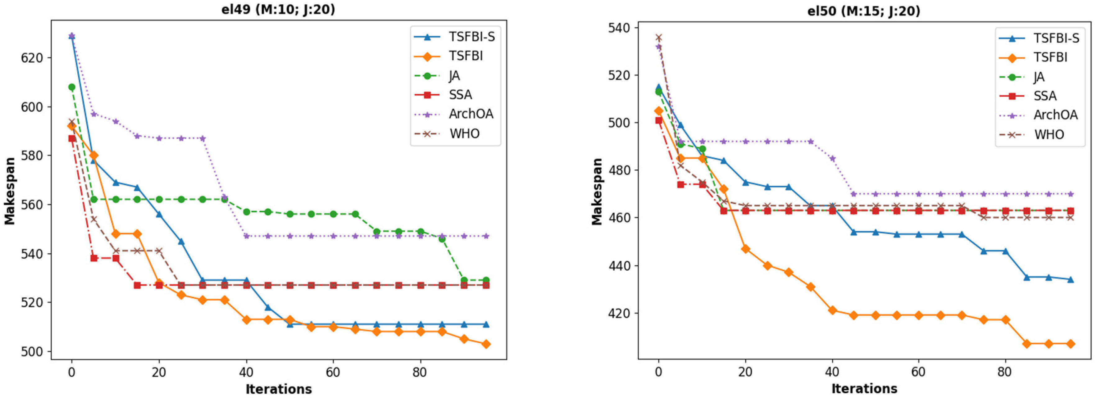
The initial test utilized el41–el50 for the verification of the compared encoding methods [56], including the TSFBI-S, where the TSFBI-S represented our proposed TSFBI framework but utilized an alternative encoding method adopted from Shi et al. [57] for comparison purposes. This comparison aimed to validate the effectiveness of the hybrid encoding technique proposed in this paper. To further illustrate the potential of the proposed codec technique in solving flexible job shop scheduling problems, newer metaheuristic algorithms were selected separately according to the classification of optimization algorithms presented in article [57]. These included the JA [58] and SSA [59] algorithms based on animal social behavior, the ArchOA [60] algorithm based on physical processes, and the WHO [61] algorithm inspired by biology.
The experimental results are shown in Figure 6, Figure 7 and 
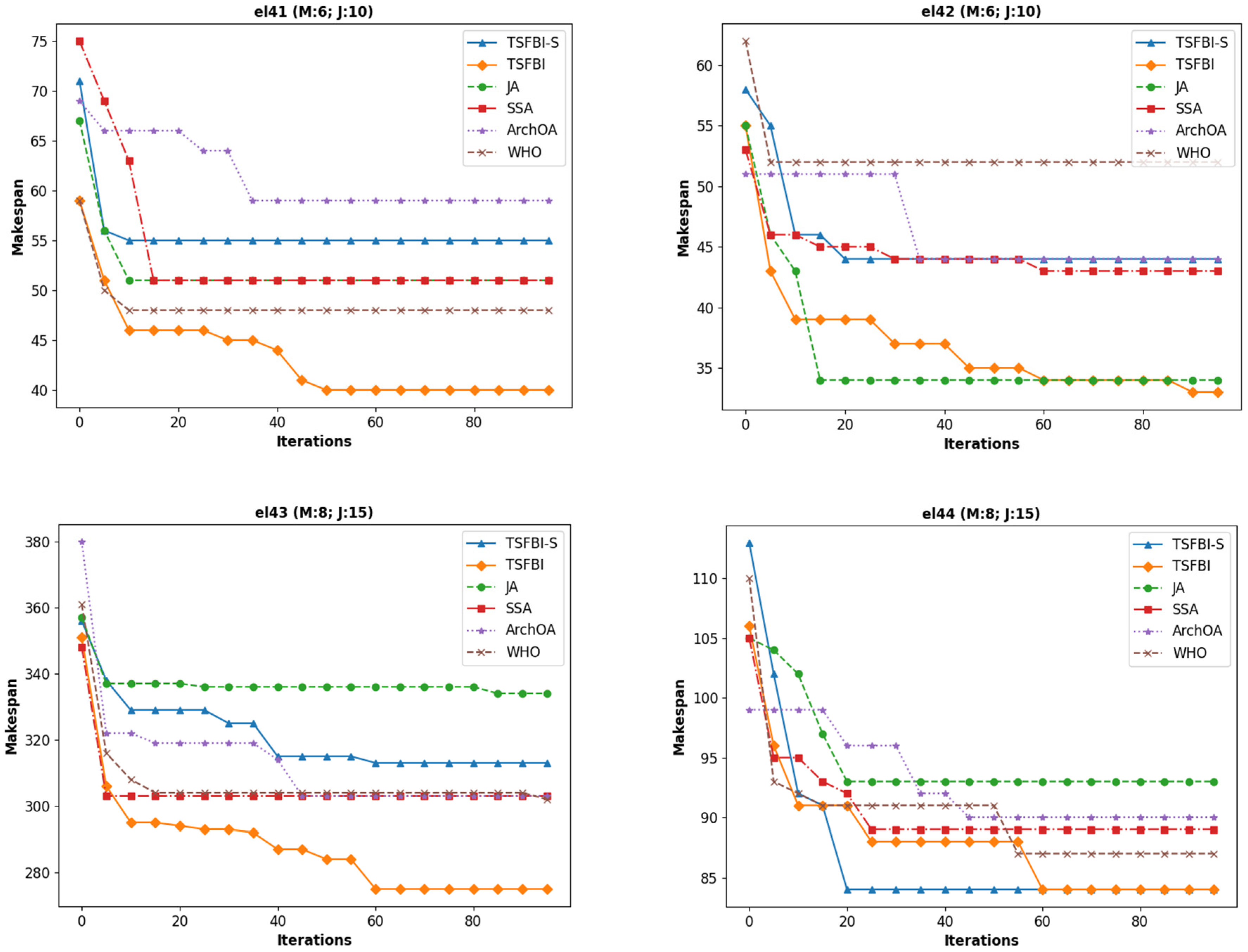
Figure 8, where the x-axis of each figure represents the number of iterations completed by the algorithm, the y-axis represents the maximum completion time, and the captions refer to the different examples.
We know from the experimental results that the proposed codec method facilitates the rapid application of new continuous optimization algorithms in combinatorial optimization problems such as the DRFJSP, and the FBI algorithm always obtained better solutions when solving the FJSP than the other algorithms.
The results presented in Figure 6, Figure 7 and Figure 8 demonstrate the effectiveness of the proposed hybrid encoding method, enabling the application of continuous optimization algorithms like the FBI to the discrete DRFJSP. Notably, the FBI algorithm consistently converged to better solutions (lower makespan) than those of JA, SSA, ArchOA, and WHO within the same number of iterations across most Mk benchmark instances, highlighting its potential for solving complex scheduling problems efficiently.
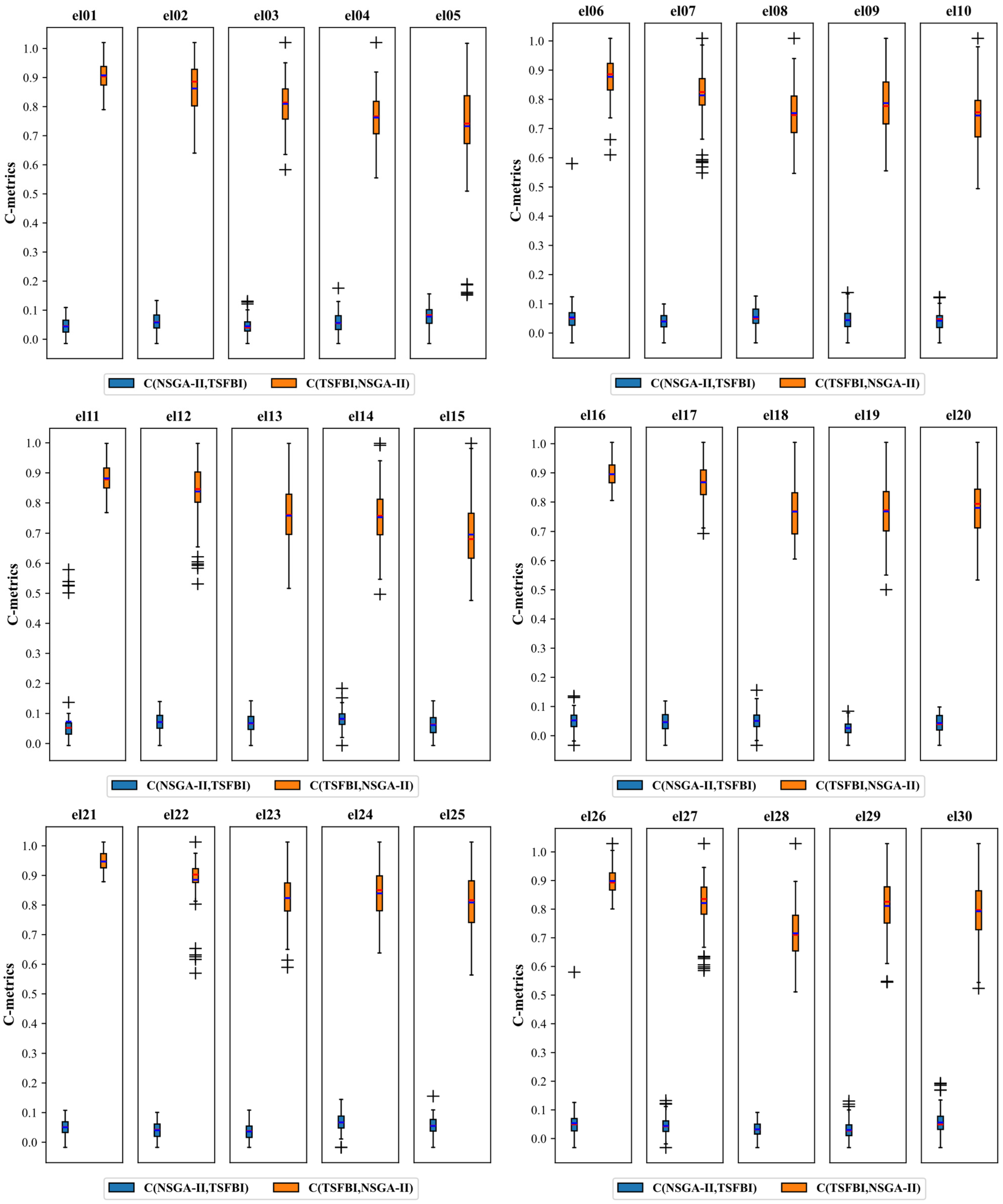
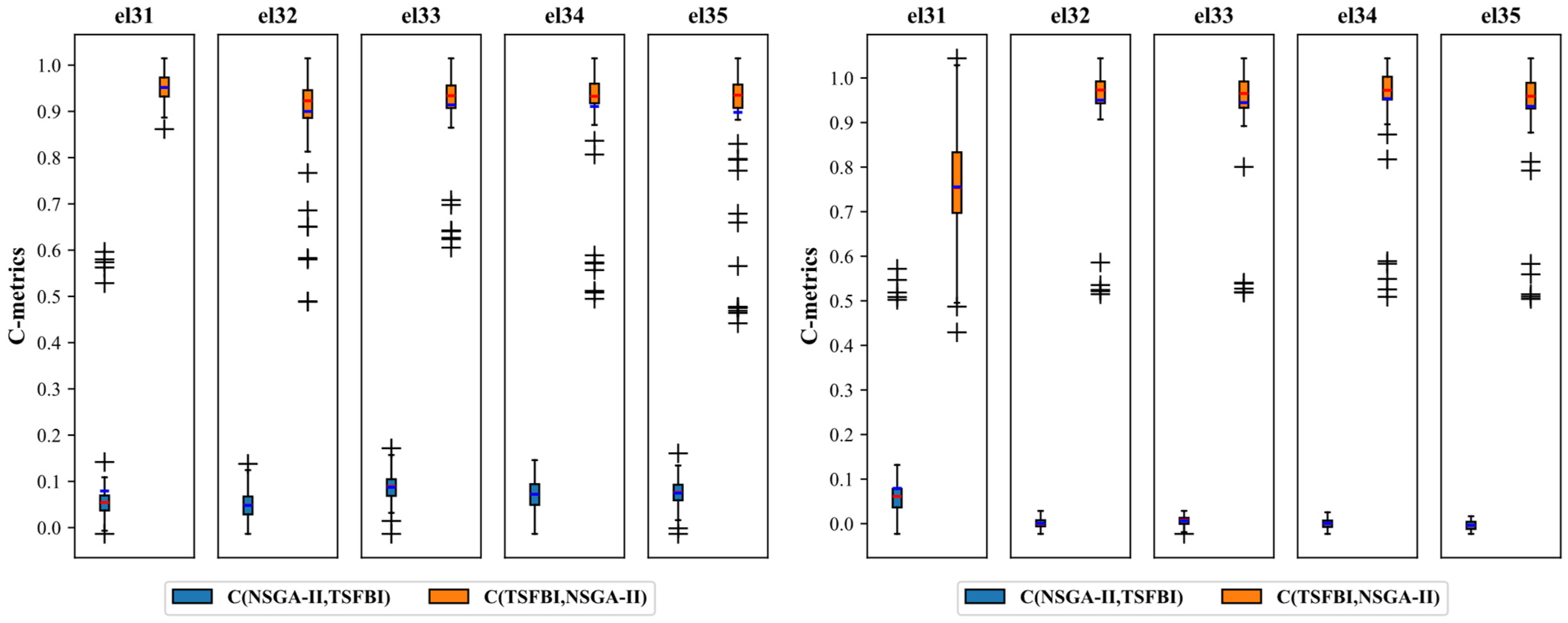
The extended instances (el01–el40) were optimized using the TSFBI and the NSGA-II, and three metrics, the C-metric, SM, and HVR, were statistically calculated. The statistics for the C-metrics are shown in Figure 9. To visually demonstrate the variances in the distribution of the solutions produced by the TSFBI and NSGA-II, we utilized box plots. Each plot compares five instances, with a total of eight plots encompassing instances el01–el40. The x-axis of each plot depicts the TSFBI and NSGA-II categories, while the y-axis represents the C-metrics.
Figure 9 illustrates the C-metric comparison between the TSFBI and NSGA-II. Recalling that C(A, B) represents the fraction of solutions in B dominated by solutions in A, the generally high values observed for C(TSFBI, NSGA-II) indicate that a large proportion of NSGA-II solutions were dominated by TSFBI solutions. Conversely, the generally low values for C(NSGA-II, TSFBI) indicate that only a small proportion of TSFBI solutions were dominated by NSGA-II solutions. This demonstrates that the TSFBI algorithm achieved superior dominance performance in acquiring Pareto sets compared to the NSGA-II algorithm.
As shown in Table 6, where the best value is in bold, the solutions obtained by the TSFBI were better than those obtained by NSGA-II in terms of their distribution, convergence, and diversity.
As shown in Figure 9 and Table 6, the TSFBI algorithm significantly outperformed the well-established NSGA-II algorithm across the tested instances (el01–el40). Specifically, the superior C-metric values indicate that the TSFBI generates Pareto sets with better dominance characteristics. Furthermore, the lower SM values suggest a more uniform distribution of solutions along the Pareto front, while the higher HVR values demonstrate better convergence and the wider coverage of the objective space. These combined results strongly suggest that the TSFBI is more effective than NSGA-II in finding a diverse and high-quality set of trade-off solutions for the DRFJSP, thus offering better support for decision-making regarding the scheduling efficiency and cost.

5.5. Experiment III on AHP Decision-Making Process

The Pareto solutions obtained using the TSFBI for the optimization calculation for the simple case are shown in Figure 10. This study focused on two objectives, namely the completion time and worker cost, with a particular emphasis on the worker cost. The importance of these objectives was determined by assigning them ratings from 1 to 9 to construct the judgment matrix A. Therefore, the decision-maker’s preference for minimizing the worker cost was set at 8, while a rating of 1 is assigned to the minimization of the makespan. Using the weight calculation steps in Section 4.2, the weight vector was calculated:
w = 1 9 , 8 9
To clarify the calculation process, for each Pareto solution, i (visualized in Figure 10), the objective values ( f 1 i for the makespan, f 2 i for the worker cost) were determined. These objective values were then normalized (using a specific normalization method, e.g., using the sum in Equation (24)). The normalized values for solution i were plugged into Equation (24), along with the decision-maker’s weight vector w = (1/9, 8/9) (Equation (30)) derived from the judgment matrix A (Equation (31)). This calculation yielded the A A H P score for solution i, as is present in the vector in Equation (32), and based on Equation (32), the satisfaction vector was calculated, and the best value was achieved by solution 5. Solution 5 refers to the specific Pareto-optimal solution corresponding to the fifth score (0. 99234093) in the A A H P vector. Based on the AHP analysis aiming to maximize this score, it was identified as the preferred solution in this context.
A = f 1 f 2 f 1 1 1 / 8 f 2 8 1
A A H P = { 0.86110818 ,   0.92017231 ,   0.78182572 ,   0.97808061 ,   0.99234093 ,   0.97210737 ,   0.88652432 ,   0.85569519 ,   0.83617673 ,   0.89648891 ,   0.22739165 ,   0.86686443 ,   0.87721493 ,   0.8823313 ,   0.14896923 ,   0.88075093 ,   0.76343755 ,   0 ,   0.1321474 ,   0.88562199 ,   0.81801527 ,   0.94954383 ,   0.88776956 ,   0.48362909 ,   0.90787544 ,   0.44769671 ,   0.67799616 ,   0.55448318 ,   0.46445823 ,   0.9345759 } .
In this illustrative example, the preference for minimizing the worker cost (rating of 8) over the makespan (rating of 1) was assumed based on a hypothetical scenario where cost control was a primary concern for the decision-maker. In a real-world application, this judgment matrix would be established based on the actual preferences and strategic goals of the factory management. Different managers or changing priorities might lead to a different matrix A and consequently a different final solution selection. Future studies could explore the impact of varying weight assignments on the final scheduling decision through sensitivity analysis to assess the robustness of the chosen solution under different preference scenarios.
Figure 10 illustrates the Pareto front obtained for the simple case, clearly showing the trade-off between minimizing the makespan (f1) and minimizing worker costs (f2). For instance, solutions in the lower-left part of the front offered a shorter makespan but incurred higher worker costs, while solutions in the upper-right part achieved lower worker costs at the expense of a longer makespan. Solution 4, selected through the AHP with a strong preference towards minimizing worker costs (weight of 8/9 for f2), represented the most satisfactory compromise according to this specific preference structure, even though it did not have the absolute lowest makespan or the absolute lowest cost among all the Pareto solutions.

6. Conclusions

With increasing labor costs and the need for fine-grained production management, the consideration of human and machine resources in the scheduling process is receiving increasing attention. This article presents a human-centered approach to addressing the dual-resource flexible job shop scheduling problem and its solution. It explores the utilization of and dependence on human resources from two perspectives. First, the article discusses the incorporation of employees’ flexible working hours, constrained by minimum and maximum limits and often linked to work–life balance considerations, into the scheduling model. Second, it proposes a two-stage algorithm, drawing on the forensic-based investigation algorithm of human problem-solving behavior, to effectively solve the dual-resource flexible job shop scheduling problem (DRFJSP). By delegating scheduling decisions to managers, the method enables the creation of more flexible and dependable scheduling plans. By effectively optimizing both the makespan and worker costs, the proposed TSFBI algorithm provides manufacturers with valuable tools to improve the scheduling efficiency (reducing production lead times) and enhance cost-effectiveness (controlling labor expenditures) in complex dual-resource-constrained environments. The generation of a Pareto front allows for informed decision-making based on the desired balance between these critical objectives. The main findings of the paper are as follows:
  • In this paper, we discuss the impact of flexible working time arrangements on worker costs and production efficiency and formally describe the problem in a multi-objective mixed-integer linear programming model.
  • A two-stage approach based on the forensic-based investigation (TSFBI) is proposed to solve the model. First, the mapping relationship between the scheduling solution and the suspect vector of the DRFJSP is constructed using a hybrid codec approach, which ensures that the suspect vector is equivalent to a feasible scheduling solution. Second, the dominance relation of the solution is determined through fast non-dominated sorting, and a quantitative comparison operator is used to ensure the population’s diversity while not increasing the time complexity. Finally, the Pareto solutions are examined analytically through the AHP to obtain a satisfactory scheduling solution.
  • Three experiments were designed to verify the performance of the proposed TSFBI algorithm. The first experiment demonstrated the accuracy of the mixed-integer programming model established. The second experiment verified the effectiveness and efficiency of the proposed TSFBI algorithm. Comparing its results against those of the widely used NSGA-II algorithm demonstrated the TSFBI’s superiority in handling the DRFJSP, particularly in terms of the dominance, distribution, convergence, and diversity of the obtained Pareto solutions (as indicated by the C-metric, SM, and HVR, respectively). Furthermore, comparisons with several other recent metaheuristics (JA, SSA, ArchOA, WHO) using the proposed encoding method indicated the strong performance of the underlying FBI optimization engine for this type of problem. The third experiment examined the use of the AHP to obtain the optimal solution and proved the ability of the TSFBI to obtain the most suitable scheduling solution.
Despite the promising results, this study has several limitations that warrant acknowledgment. Firstly, the DRFJSP model operates under deterministic assumptions, neglecting stochastic events common in real manufacturing, such as machine breakdowns, processing time variability, or unexpected worker unavailability. Secondly, the validation primarily relied on benchmark instances; further testing with real-world industrial data is needed to confirm the practical applicability and robustness of the model and algorithm. Thirdly, certain operational details, such as worker skill levels, learning effects, or shift changeover times, were simplified or omitted. Furthermore, future research could broaden the comparative analysis by including the consideration of other established multi-objective algorithms, such as MOEA/D and SPEA2, to provide a more comprehensive benchmark of the TSFBI algorithm’s performance. Finally, while a preliminary sensitivity analysis was performed, a more comprehensive investigation into parameter tuning for the TSFBI algorithm could potentially further enhance its performance. To conclude, our work here has practical significance regarding the proposed model and research implications. Future research will focus on addressing these limitations by incorporating stochastic elements into the model (e.g., using simulation-based optimization or robust optimization techniques), validating the approach using industrial case studies, considering more detailed human factors (like skills and fatigue), and conducting extensive parameter optimization.

Author Contributions

All authors contributed to the study’s conception and design. Conceptualization, Y.Z. and P.L.; data curation, Y.Z. and C.F.; funding acquisition, P.L., J.H. (Jianmin Hu), and Q.L.; investigation, P.L. and J.H. (Jianmin Hu); methodology, Y.Z., P.L., Q.L. and J.H. (Jiwei Hu); supervision, J.H. (Jianmin Hu) and Q.L.; validation, C.F.; writing—original draft, Y.Z.; writing—review and editing, Y.Z., P.L., J.H. (Jianmin Hu) and J.H. (Jiwei Hu). All authors have read and agreed to the published version of the manuscript.

Funding

This research was funded by the Natural Science Foundation of Hubei Province of China under Grant 2025AFA055 and the National Key Research and Development Program of China under Grant 2020YFB1710804.

Data Availability Statement

The data supporting the results of this study are described in the first paragraph of Section 5.1.

Conflicts of Interest

The authors confirm that there are no conflicts of interest.

References

  1. Escamilla-Serna, N.J.; Seck-Tuoh-Mora, J.C.; Medina-Marin, J.; Barragan-Vite, I.; Corona-Armenta, J.R. A Hybrid Search Using Genetic Algorithms and Random-Restart Hill-Climbing for Flexible Job Shop Scheduling Instances with High Flexibility. Appl. Sci. 2022, 12, 8050. [Google Scholar] [CrossRef]
  2. Mourtzis, D. Simulation in the Design and Operation of Manufacturing Systems: State of the Art and New Trends. Int. J. Prod. Res. 2020, 58, 1927–1949. [Google Scholar] [CrossRef]
  3. Gong, G.; Chiong, R.; Deng, Q.; Han, W.; Zhang, L.; Lin, W.; Li, K. Energy-Efficient Flexible Flow Shop Scheduling with Worker Flexibility. Expert Syst. Appl. 2020, 141, 112902. [Google Scholar] [CrossRef]
  4. Li, Z.; Pei, J.; Yan, P.; Zhou, Y.; Pardalos, P.M. Dynamic Resource Allocation and Collaborative Scheduling in R&D and Manufacturing Processes of High-End Equipment with Budget Constraint. Optim. Lett. 2023, 17, 955–980. [Google Scholar] [CrossRef]
  5. Andrade-Pineda, J.L.; Canca, D.; Gonzalez-R, P.L.; Calle, M. Scheduling a Dual-Resource Flexible Job Shop with Makespan and Due Date-Related Criteria. Ann. Oper. Res. 2020, 291, 5–35. [Google Scholar] [CrossRef]
  6. Zhang, S.; Du, H.; Borucki, S.; Jin, S.; Hou, T.; Li, Z. Dual Resource Constrained Flexible Job Shop Scheduling Based on Improved Quantum Genetic Algorithm. Machines 2021, 9, 108. [Google Scholar] [CrossRef]
  7. Wang, H.; Alidaee, B.; Ortiz, J.; Wang, W. The Multi-Skilled Multi-Period Workforce Assignment Problem. Int. J. Prod. Res. 2021, 59, 5477–5494. [Google Scholar] [CrossRef]
  8. Lott, Y. Does Flexibility Help Employees Switch Off from Work? Flexible Working-Time Arrangements and Cognitive Work-to-Home Spillover for Women and Men in Germany. Soc. Indic. Res. 2020, 151, 471–494. [Google Scholar] [CrossRef]
  9. Jarrahi, M.H.; Newlands, G.; Butler, B.; Savage, S.; Lutz, C.; Dunn, M.; Sawyer, S. Flexible Work and Personal Digital Infrastructures. Commun. ACM 2021, 64, 72–79. [Google Scholar] [CrossRef]
  10. Destouet, C.; Tlahig, H.; Bettayeb, B.; Mazari, B. Flexible Job Shop Scheduling Problem under Industry 5.0: A Survey on Human Reintegration, Environmental Consideration and Resilience Improvement. J. Manuf. Syst. 2023, 67, 155–173. [Google Scholar] [CrossRef]
  11. Wang, B.; Zheng, P.; Yin, Y.; Shih, A.; Wang, L. Toward Human-Centric Smart Manufacturing: A Human-Cyber-Physical Systems (HCPS) Perspective. J. Manuf. Syst. 2022, 63, 471–490. [Google Scholar] [CrossRef]
  12. Sakai, H. New Human-Centered Production System-Building an Integrated Human Management System. Int. J. Appl. Math. Comput. Sci. Syst. Eng. 2021, 3, 116–123. [Google Scholar] [CrossRef]
  13. Liaqait, R.A.; Hamid, S.; Warsi, S.S.; Khalid, A. A Critical Analysis of Job Shop Scheduling in Context of Industry 4.0. Sustainability 2021, 13, 7684. [Google Scholar] [CrossRef]
  14. Gong, G.; Deng, Q.; Gong, X.; Liu, W.; Ren, Q. A New Double Flexible Job-Shop Scheduling Problem Integrating Processing Time, Green Production, and Human Factor Indicators. J. Clean. Prod. 2018, 174, 560–576. [Google Scholar] [CrossRef]
  15. Yu, F.; Lu, C.; Zhou, J.; Yin, L. Mathematical Model and Knowledge-Based Iterated Greedy Algorithm for Distributed Assembly Hybrid Flow Shop Scheduling Problem with Dual-Resource Constraints. Expert Syst. Appl. 2024, 239, 122434. [Google Scholar] [CrossRef]
  16. Mlekusch, J.; Hartl, R.F. The Dual-Resource-Constrained Re-Entrant Flexible Flow Shop a Constraint Programming Approach and a Hybrid Genetic Algorithm. Int. J. Prod. Res. 2025, 63, 1803–1824. [Google Scholar] [CrossRef]
  17. Renna, P.; Thürer, M.; Stevenson, M. A Game Theory Model Based on Gale-Shapley for Dual-Resource Constrained (DRC) Flexible Job Shop Scheduling. Int. J. Ind. Eng. Comput. 2020, 11, 173–184. [Google Scholar] [CrossRef]
  18. Li, H.; Peng, J.; Wang, X. An Efficient Two-Stage Optimization Algorithm for a Flexible Job Shop Scheduling Problem with Worker Shift Arrangement. Comput. Oper. Res. 2024, 171, 106785. [Google Scholar] [CrossRef]
  19. Xiao, S.; Wu, Z.; Yu, S. A Two-Stage Assignment Strategy for the Robust Scheduling of Dual-Resource Constrained Stochastic Job Shop Scheduling Problems. IFAC-PapersOnLine 2019, 52, 421–426. [Google Scholar] [CrossRef]
  20. Li, H.; Wu, X. A Survival Duration-Guided NSGA-III for Sustainable Flexible Job Shop Scheduling Problem Considering Dual Resources. IET Collab. Intell. Manuf. 2021, 3, 119–130. [Google Scholar] [CrossRef]
  21. Wei, S.; Tang, H.; Li, X.; Lei, D.; Wang, X.V. An Improved Memetic Algorithm for Multi-Objective Resource-Constrained Flexible Job Shop Inverse Scheduling Problem: An Application for Machining Workshop. J. Manuf. Syst. 2024, 74, 264–290. [Google Scholar] [CrossRef]
  22. Berti, N.; Finco, S.; Battaïa, O.; Delorme, X. Ageing Workforce Effects in Dual-Resource Constrained Job-Shop Scheduling. Int. J. Prod. Econ. 2021, 237, 108151. [Google Scholar] [CrossRef]
  23. Seifi, C.; Schulze, M.; Zimmermann, J. A New Mathematical Formulation for a Potash-Mine Shift Scheduling Problem with a Simultaneous Assignment of Machines and Workers. Eur. J. Oper. Res. 2021, 292, 27–42. [Google Scholar] [CrossRef]
  24. Santos, F.; Fukasawa, R.; Ricardez-Sandoval, L. An Integrated Machine Scheduling and Personnel Allocation Problem for Large-Scale Industrial Facilities Using a Rolling Horizon Framework. Optim. Eng. 2020, 22, 2603–2626. [Google Scholar] [CrossRef]
  25. Chung, H.; van der Lippe, T. Flexible Working, Work–Life Balance, and Gender Equality: Introduction. Soc. Indic. Res. 2020, 151, 365–381. [Google Scholar] [CrossRef]
  26. Baridula, V.; Adanma, M.-N. Flexible work practices and employee retention in manufacturing companies in Nigeria. Int. J. Adv. Acad. Res. 2021, 7, 13–33. [Google Scholar] [CrossRef]
  27. Delgoshaei, A.; Ariffin, M.K.A.M.; Maleki, S.; Leman, Z. Review Evolution of Dual-Resource-Constrained Scheduling Problems in Manufacturing Systems: Modeling and Scheduling Methods’ Trends. Soft Comput. Fusion Found. Methodol. Appl. 2023, 27, 18489–18528. [Google Scholar] [CrossRef]
  28. Abderrahim, M.; Bekrar, A.; Trentesaux, D.; Aissani, N.; Bouamrane, K. Bi-Local Search Based Variable Neighborhood Search for Job-Shop Scheduling Problem with Transport Constraints. Optim. Lett. 2022, 16, 255–280. [Google Scholar] [CrossRef]
  29. Zhang, X.; Pang, Y.; Kang, Y.; Chen, W.; Fan, L.; Jin, H.; Yang, Q. No Free Lunch Theorem for Privacy-Preserving LLM Inference. Artif. Intell. 2025, 341, 104293. [Google Scholar] [CrossRef]
  30. Jiang, T.; Zhu, H.; Gu, J.; Liu, L.; Song, H. A Discrete Animal Migration Algorithm for Dual-Resource Constrained Energy-Saving Flexible Job Shop Scheduling Problem. J. Intell. Fuzzy Syst. 2022, 42, 3431–3444. [Google Scholar] [CrossRef]
  31. Nguyen, T.; Nguyen, G.; Nguyen, B.M. EO-CNN: An Enhanced CNN Model Trained by Equilibrium Optimization for Traffic Transportation Prediction. Procedia Comput. Sci. 2020, 176, 800–809. [Google Scholar] [CrossRef]
  32. Lu, X.; Lu, C. Mixed-Production Flexible Assembly Job Shop Scheduling Considering Parallel Assembly Sequence Variations under Dual-Resource Constraints Using Multi-Objective Hybrid Memetic Algorithm. Comput. Oper. Res. 2025, 176, 106932. [Google Scholar] [CrossRef]
  33. Zhang, Z.; Li, X.; Gao, L.; Liu, Q.; Huang, J. Tackling Dual-Resource Flexible Job Shop Scheduling Problem in the Production Line Reconfiguration Scenario: An Efficient Meta-Heuristic with Critical Path-Based Neighborhood Search. Adv. Eng. Inform. 2025, 65, 103282. [Google Scholar] [CrossRef]
  34. Liu, L.; Song, H.; Jiang, T.; Deng, G.; Gong, Q. Modified Biology Migration Algorithm for Dual-Resource Energy-Saving Flexible Job Shop Scheduling Problem. Jisuanji Jicheng Zhizao Xitong Comput. Integr. Manuf. Syst. CIMS 2024, 30, 3125–3141. [Google Scholar]
  35. Akbar, M.; Irohara, T. NSGA Families for Solving a Dual Resource-Constrained Problem to Optimize the Total Tardiness and Labor Productivity in the Spirit of Sustainability. Comput. Ind. Eng. 2024, 188, 109883. [Google Scholar] [CrossRef]
  36. Chou, J.-S.; Nguyen, N.-M. FBI Inspired Meta-Optimization. Appl. Soft Comput. 2020, 93, 106339. [Google Scholar] [CrossRef]
  37. Hoang, N.-D.; Huynh, T.-C.; Tran, V.-D. Computer Vision-Based Patched and Unpatched Pothole Classification Using Machine Learning Approach Optimized by Forensic-Based Investigation Metaheuristic. Complexity 2021, 2021, e3511375. [Google Scholar] [CrossRef]
  38. Nguyen, D.-T.; Chou, J.-S.; Tran, D.-H. Integrating a Novel Multiple-Objective FBI with BIM to Determine Tradeoff among Resources in Project Scheduling. Knowl.-Based Syst. 2022, 235, 107640. [Google Scholar] [CrossRef]
  39. Fan, J.; Shen, W.; Gao, L.; Zhang, C.; Zhang, Z. A Hybrid Jaya Algorithm for Solving Flexible Job Shop Scheduling Problem Considering Multiple Critical Paths. J. Manuf. Syst. 2021, 60, 298–311. [Google Scholar] [CrossRef]
  40. Liu, Q.; Li, X.; Liu, H.; Guo, Z. Multi-Objective Metaheuristics for Discrete Optimization Problems: A Review of the State-of-the-Art. Appl. Soft Comput. 2020, 93, 106382. [Google Scholar] [CrossRef]
  41. Dauzère-Pérès, S.; Ding, J.; Shen, L.; Tamssaouet, K. The Flexible Job Shop Scheduling Problem: A Review. Eur. J. Oper. Res. 2024, 314, 409–432. [Google Scholar] [CrossRef]
  42. Mar-Ortiz, J.; Ruiz Torres, A.J.; Adenso-Díaz, B. Scheduling in Parallel Machines with Two Objectives: Analysis of Factors That Influence the Pareto Frontier. Oper. Res. 2022, 22, 4585–4605. [Google Scholar] [CrossRef]
  43. Marques, E.L.; Coelho, V.N.; Coelho, I.M.; Satoru Ochi, L.; Maculan, N.; Mladenović, N.; Coelho, B.N. A Two-Phase Multi-Objective Metaheuristic for a Green UAV Grid Routing Problem. Optim. Lett. 2023, 17, 2233–2256. [Google Scholar] [CrossRef]
  44. Moslem, S. A Novel Parsimonious Spherical Fuzzy Analytic Hierarchy Process for Sustainable Urban Transport Solutions. Eng. Appl. Artif. Intell. 2024, 128, 107447. [Google Scholar] [CrossRef]
  45. Zhang, C.; Zhang, C.; Zhuang, J.; Han, H.; Yuan, B.; Liu, J.; Yang, K.; Zhuang, S.; Li, R. Evaluation of Cloud 3D Printing Order Task Execution Based on the AHP-TOPSIS Optimal Set Algorithm and the Baldwin Effect. Micromachines 2021, 12, 801. [Google Scholar] [CrossRef]
  46. Yuan, M.; Li, Y.; Zhang, L.; Pei, F. Research on Intelligent Workshop Resource Scheduling Method Based on Improved NSGA-II Algorithm. Robot. Comput.-Integr. Manuf. 2021, 71, 102141. [Google Scholar] [CrossRef]
  47. Demir, Y.; Kürşat İşleyen, S. Evaluation of Mathematical Models for Flexible Job-Shop Scheduling Problems. Appl. Math. Model. 2013, 37, 977–988. [Google Scholar] [CrossRef]
  48. Deb, K.; Pratap, A.; Agarwal, S.; Meyarivan, T. A Fast and Elitist Multiobjective Genetic Algorithm: NSGA-II. IEEE Trans. Evol. Comput. 2002, 6, 182–197. [Google Scholar] [CrossRef]
  49. Li, D.; Zhang, C.; Shao, X.; Lin, W. A Multi-Objective TLBO Algorithm for Balancing Two-Sided Assembly Line with Multiple Constraints. J. Intell. Manuf. 2016, 27, 725–739. [Google Scholar] [CrossRef]
  50. Hurink, J.; Jurisch, B.; Thole, M. Tabu Search for the Job-Shop Scheduling Problem with Multi-Purpose Machines. OR Spektrum 1994, 15, 205–215. [Google Scholar] [CrossRef]
  51. Brandimarte, P. Routing and Scheduling in a Flexible Job Shop by Tabu Search. Ann. Oper. Res. 1993, 41, 157–183. [Google Scholar] [CrossRef]
  52. Pezzella, F.; Morganti, G.; Ciaschetti, G. A Genetic Algorithm for the Flexible Job-Shop Scheduling Problem. Comput. Oper. Res. 2008, 35, 3202–3212. [Google Scholar] [CrossRef]
  53. Liu, M.; Lv, J.; Du, S.; Deng, Y.; Shen, X.; Zhou, Y. Multi-Resource Constrained Flexible Job Shop Scheduling Problem with Fixture-Pallet Combinatorial Optimisation. Comput. Ind. Eng. 2024, 188, 109903. [Google Scholar] [CrossRef]
  54. Caldeira, R.H.; Gnanavelbabu, A. A Pareto Based Discrete Jaya Algorithm for Multi-Objective Flexible Job Shop Scheduling Problem. Expert Syst. Appl. 2021, 170, 114567. [Google Scholar] [CrossRef]
  55. Achterberg, T. What’s New in Gurobi 9.0. Available online: https://www.google.com.hk/url?sa=t&source=web&rct=j&opi=89978449&url=https://cdn.gurobi.com/wp-content/uploads/Gurobi-9.0-Overview-Webinar-Slides-1.pdf&ved=2ahUKEwjgmtfT_faMAxViaPUHHUX-Bl8QFnoECBgQAQ&usg=AOvVaw0hD8tKEukvGHPKlGz6NHpI (accessed on 28 March 2025).
  56. Shi, J.; Chen, M.; Ma, Y.; Qiao, F. A New Boredom-Aware Dual-Resource Constrained Flexible Job Shop Scheduling Problem Using a Two-Stage Multi-Objective Particle Swarm Optimization Algorithm. Inf. Sci. 2023, 643, 119141. [Google Scholar] [CrossRef]
  57. Cui, Y.; Geng, Z.; Zhu, Q.; Han, Y. Review: Multi-Objective Optimization Methods and Application in Energy Saving. Energy 2017, 125, 681–704. [Google Scholar] [CrossRef]
  58. Rao, R. Jaya: A Simple and New Optimization Algorithm for Solving Constrained and Unconstrained Optimization Problems. Int. J. Ind. Eng. Comput. 2016, 7, 19–34. [Google Scholar]
  59. Xue, J.; Shen, B. A Novel Swarm Intelligence Optimization Approach: Sparrow Search Algorithm. Syst. Sci. Control Eng. 2020, 8, 22–34. [Google Scholar] [CrossRef]
  60. Hashim, F.A.; Hussain, K.; Houssein, E.H.; Mabrouk, M.S.; Al-Atabany, W. Archimedes Optimization Algorithm: A New Metaheuristic Algorithm for Solving Optimization Problems. Appl. Intell. 2021, 51, 1531–1551. [Google Scholar] [CrossRef]
  61. Amali, D.G.B.; Dinakaran, M. Wildebeest Herd Optimization: A New Global Optimization Algorithm Inspired by Wildebeest Herding Behaviour. J. Intell. Fuzzy Syst. 2019, 37, 8063–8076. [Google Scholar] [CrossRef]
Figure 1. The flowchart of the TSFBI algorithm.
Mathematics 13 01432 g001
Figure 2. Encoding of the OS, MS, and WS.
Mathematics 13 01432 g002
Figure 3. Three-substring decoding method.
Mathematics 13 01432 g003
Figure 4. AHP recursive structure for multi-objective DRFJSP scheduling decisions.
Mathematics 13 01432 g004
Figure 5. Parameter sensitivity analysis of the TSFBI algorithm.
Mathematics 13 01432 g005
Figure 6. Algorithm performance comparison for el41–el44.
Mathematics 13 01432 g006
Figure 7. Algorithm performance comparison for el45–el48.
Mathematics 13 01432 g007
Figure 8. Algorithm performance comparison for el49–el50.
Mathematics 13 01432 g008
Figure 9. Experimental C-metric results for cases el41 to el50 using TSFBI and NSGA-II algorithms.
Mathematics 13 01432 g009aMathematics 13 01432 g009b
Figure 10. The Pareto solutions for the simple case.
Mathematics 13 01432 g010
Table 1. Notations for DRFJSP.
NotationsDescription
Indices:
i , i Job index
j , j Operation index
k , k Machine index
l , l Worker index
Parameters:
n Total number of jobs
n i Total number of operations for a job, i
m Total number of machines
w Total number of workers
J Set of jobs
M Set of machines
W Set of workers
a The minimum number of workers per class
b The maximum number of workers per class
O i j The jth operation of job i
M i j Set of candidate machines for O i j
W k Set of candidate workers for machine k
M A large number
S 0 The start time of the schedule
β Multiplier of general salary
S T Standard working hours of workers within a task period
L B T The lower bound of the working time for each worker within a task period
U B T The upper bound of the working time for each worker within a task period
Decision variables:
f 1 Objective function 1, which represents makespan
f 2 Objective function 2, which represents total labor cost
C m a x Makespan
C i The completion time for job i
E 1 The total cost for the standard working hours
E 2 The total cost of overtime
E 3 The total base wage of the worker
C i j k l The completion time for O i j performed on machine k by worker l
C i j 1 k l The completion time for the operation prior to O i j performed on machine k by worker l
S i j k l The start time of process O i j performed on machine k by worker l
T i j k l The processing time for O i j performed on machine k by worker l
U i j k l The unit time cost for worker l to perform O i j on machine k
B l Basic salary of worker l
v i j k l If the process O i j is performed on machine k and by worker l , the value is 1; otherwise, it is 0
z i j k l , i j k l If O i j is performed on machine k by worker l and this operation is before the operation O i j , performed on the same machine by the worker l , the value is 1; otherwise, it is 0
Table 2. The parameters of the instances.
Parameter NameValue
Unit time costU [20, 70]
Basic salaryU [800, 1200]
Task period (TP)LBCT-SE
LBT0.2 × TP
ST0.5 × TP
UBT0.7 × TP
β 2
a1
b2 × m
Table 3. The parameters of the algorithms.
Parameter NameTSFBI
population size30
maximum number of generations300
Table 4. CPU runtime with different parameters.
CaseCPU Runtime (s)
N = 10 N = 20 N = 30 N = 40 N = 50
el01402.35452.78462.91605.42802.67
el16482.82543.34555.49726.50963.20
el26563.29633.89647.07847.591123.74
Table 5. A comparison of Gurobi and the TSFBI.
InstanceSize (m, n)Scale Makespan ,   f 1 Worker   Costs ,   f 2
GurobiTSFBIDiff (%)GurobiTSFBIDiff (%)
el01 5 × 10small59059001.479 × 1051.479 × 1050
el02 65065001.837 × 1051.837 × 1050
el03 49849801.294 × 1051.294 × 1050
el04 51751701.399 × 1051.399 × 1050
el05 48648601.306 × 1051.306 × 1050
el06 5 × 15-850--2.100 × 10⁵-
el07 77477402.640 × 1052.640 × 1050
el08 77477402.198 × 1052.198 × 1050
el09 -860--1.799 × 10⁵-
el10 48648601.099 × 1051.099 × 1050
el11 5 × 20medium-1080--3.284 × 10⁵-
el12 -960--2.283 × 10⁵-
el13 -1060--2.632 × 10⁵-
el14 -1099--2.794 × 10⁵-
el15 -1100--3.039 × 10⁵-
el16 10 × 107177535.024.191 × 1054.508 × 1057.56
el17 6466805.263.571 × 1053.672 × 1052.83
el18 6636904.073.760 × 1054.245 × 10512.89
el19 6176434.213.459 × 1053.622 × 1054.71
el20 7567914.633.999 × 1054.222 × 1055.57
el21 10 × 15-853--4.720 × 10⁵-
el22 7577934.765.227 × 1055.254 × 1050.52
el23 -848--5.102 × 10⁵-
el24 -825--4.553 × 10⁵-
el25 -816--3.781 × 10⁵-
el26 10 × 20large-1089--6.125 × 10⁵-
el27 -1124--6.533 × 10⁵-
el28 -1127--6.685 × 10⁵-
el29 -1034--6.280 × 10⁵-
el30 -1085--6.440 × 10⁵-
el31 10 × 30-1550--8.427 × 10⁵-
el32 -1671--9.702 × 10⁵-
el33 -1525--7.986 × 10⁵-
el34 -1568--8.781 × 10⁵-
el35 -1594--9.093 × 10⁵-
el36 15 × 15-964--7.000 × 10⁵-
el37 -1007--7.991 × 10⁵-
el38 -957--7.559 × 10⁵-
el39 -971--7.725 × 10⁵-
el40 -968--8.709 × 10⁵-
Table 6. SM and HVR metric comparisons of the TSFBI and NSGA-II algorithms.
InstancesTSFBINSGA-II
SMHVRSMHVR
el010.471.000.610.70
el020.320.910.430.71
el030.530.890.610.56
el040.420.900.630.55
el050.410.810.710.48
el060.520.900.670.61
el070.540.920.760.57
el080.590.820.800.50
el090.430.960.880.62
el100.400.970.860.60
el110.420.980.750.67
el120.350.930.700.73
el130.450.960.760.66
el140.510.940.670.68
el150.470.960.730.71
el160.650.980.810.89
el170.570.990.830.81
el180.610.980.670.66
el190.630.990.730.57
el200.430.860.770.84
el210.550.910.640.53
el220.510.930.530.81
el230.560.920.650.71
el240.540.940.780.65
el250.610.980.830.35
el260.540.950.670.56
el270.580.970.780.61
el280.530.990.690.31
el290.610.890.710.72
el300.630.900.780.81
el310.570.920.670.73
el320.580.940.640.76
el330.600.950.700.81
el340.430.910.540.79
el350.470.970.570.24
el360.520.980.680.32
el370.530.990.650.21
el380.560.940.770.35
el390.510.920.750.44
el400.550.980.810.27
Disclaimer/Publisher’s Note: The statements, opinions and data contained in all publications are solely those of the individual author(s) and contributor(s) and not of MDPI and/or the editor(s). MDPI and/or the editor(s) disclaim responsibility for any injury to people or property resulting from any ideas, methods, instructions or products referred to in the content.

