
Scrutinizing the General Conic Equation


Abstract
1. Introduction
2. Preliminaries
2.1. Properties of the General Conic Equation and the Sign Function
- Property 1: ,
- Property 2: ,
- Property 3: .
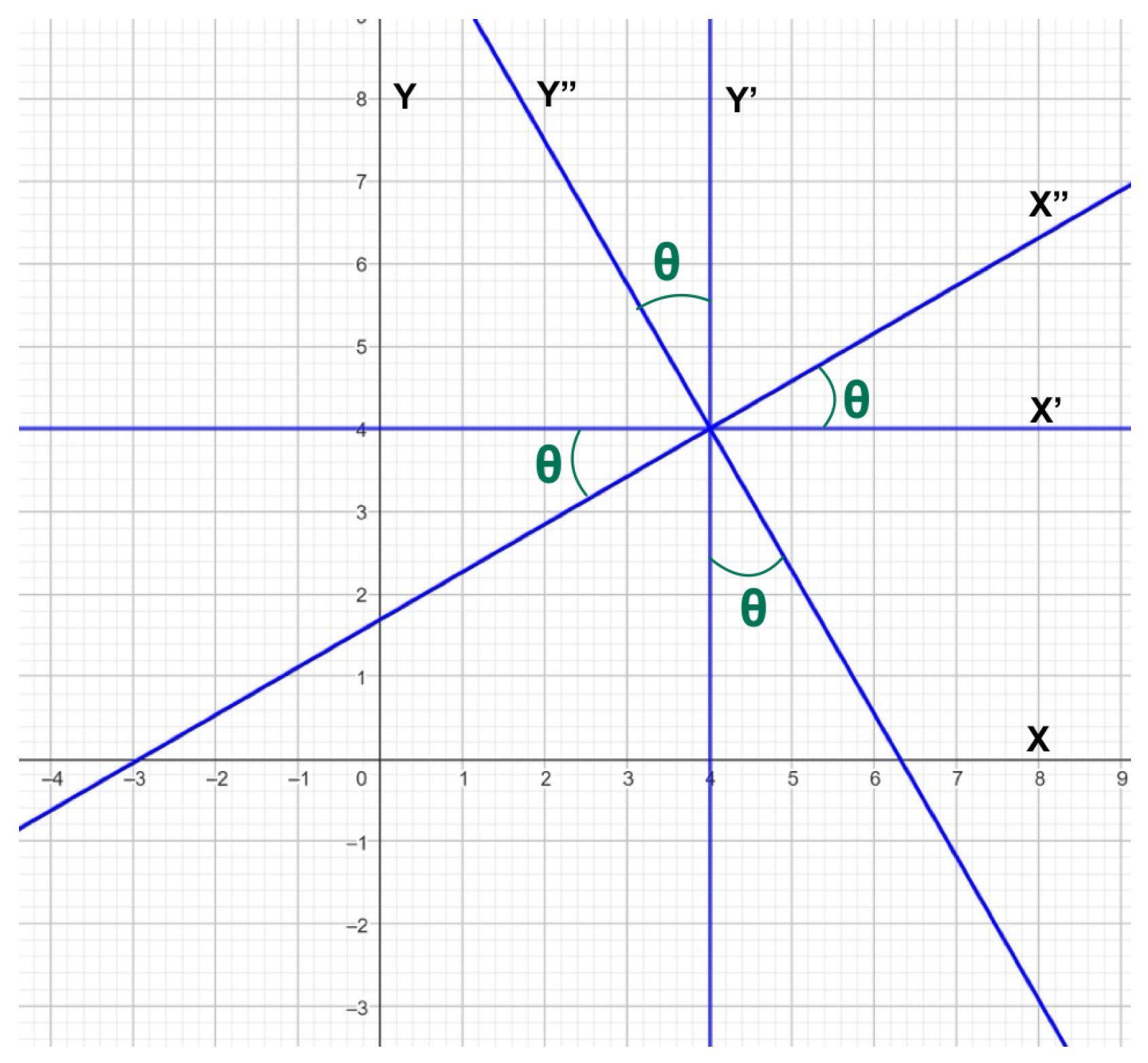
2.2. The Conic Radical and the Rotation Angle
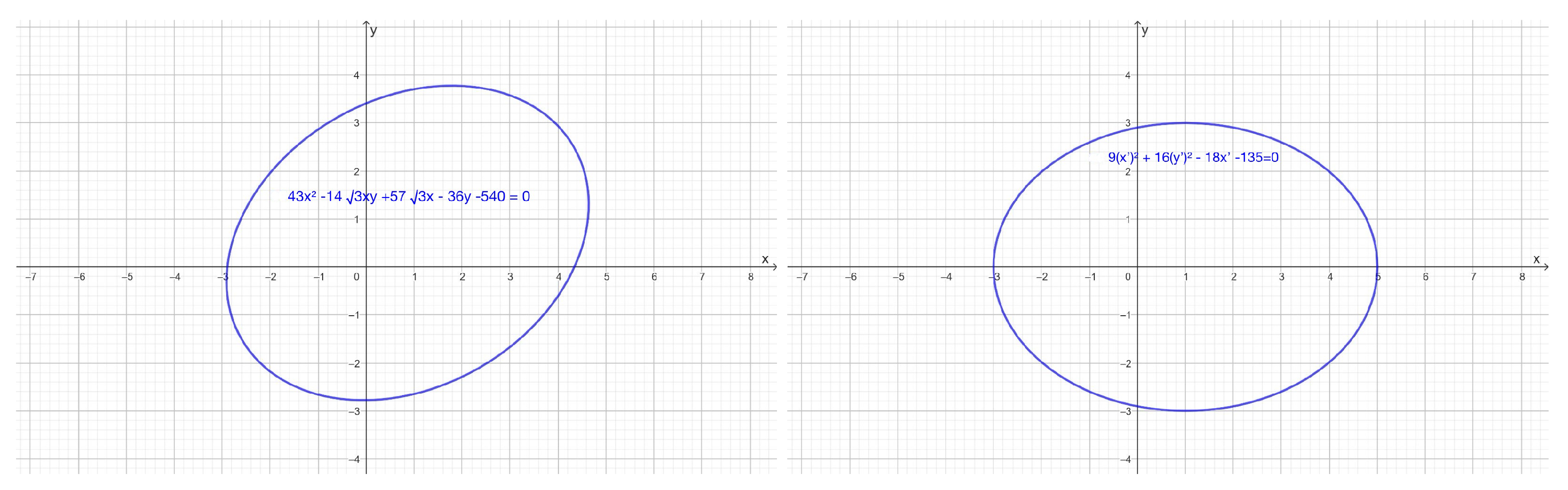
3. The Instant Simplification of the General Conic Equation Under Rotations
4. Illustrations
4.1. Two Well-Known Results
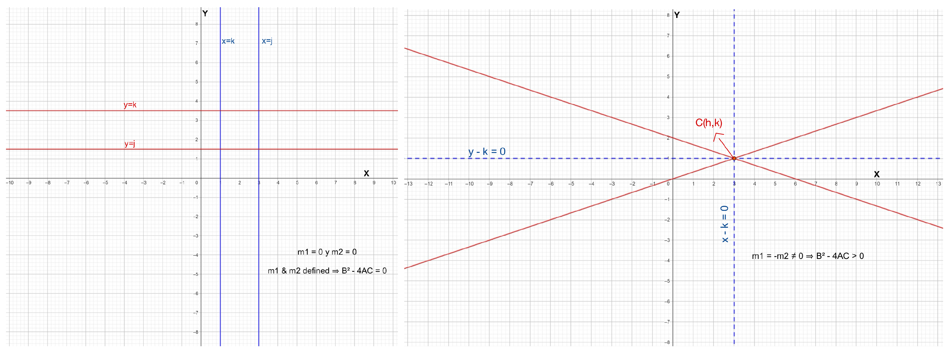
4.2. What About Degenerate Cases?
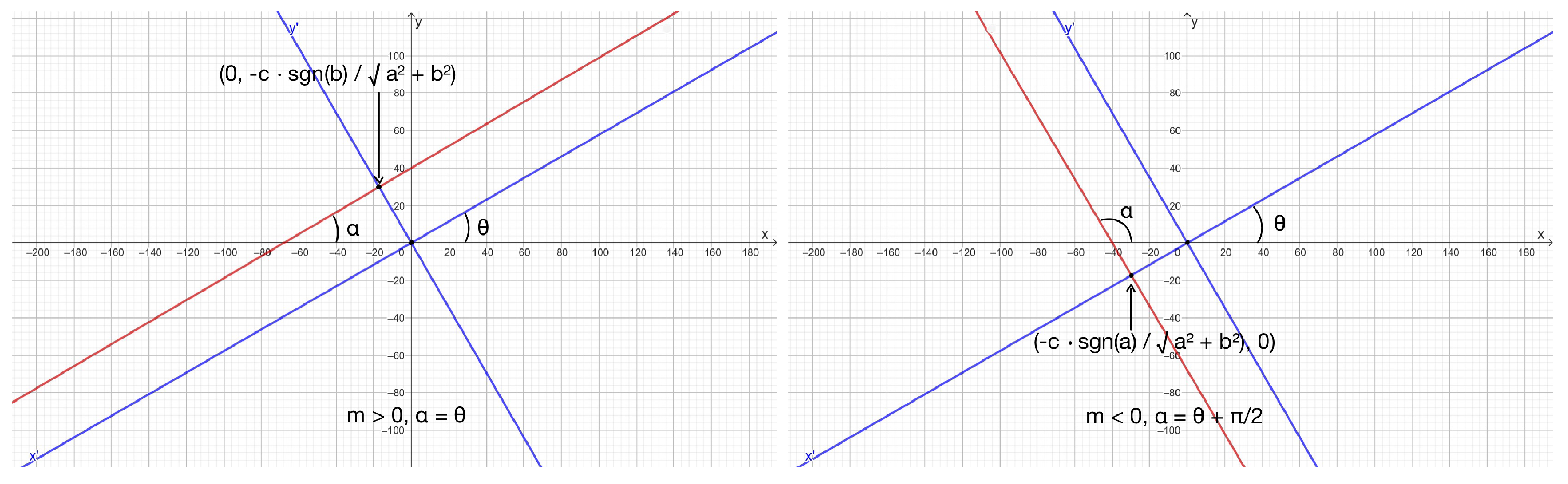
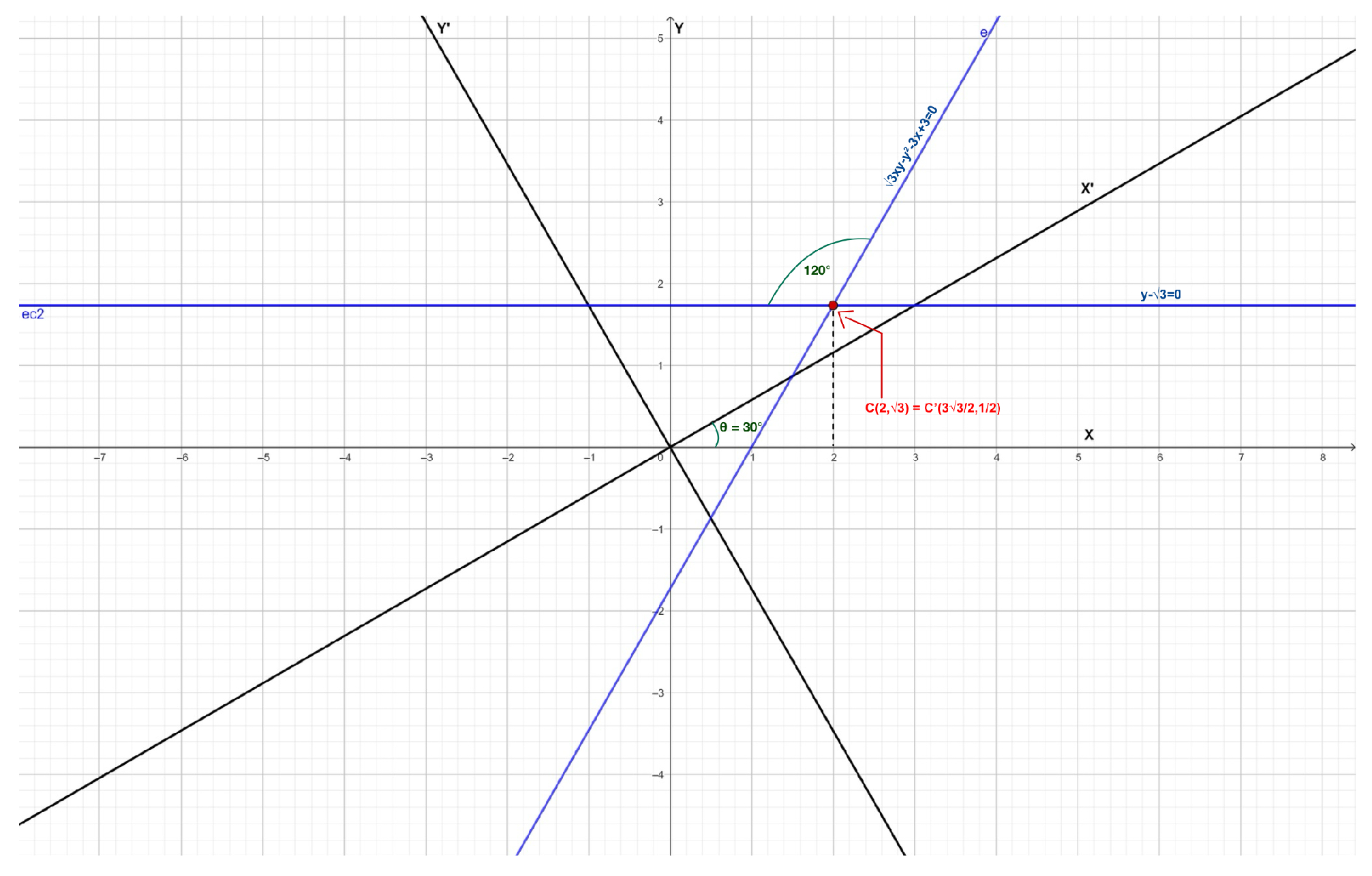
- If or both slopes are undefined, the lines are parallel to one Cartesian axis and .
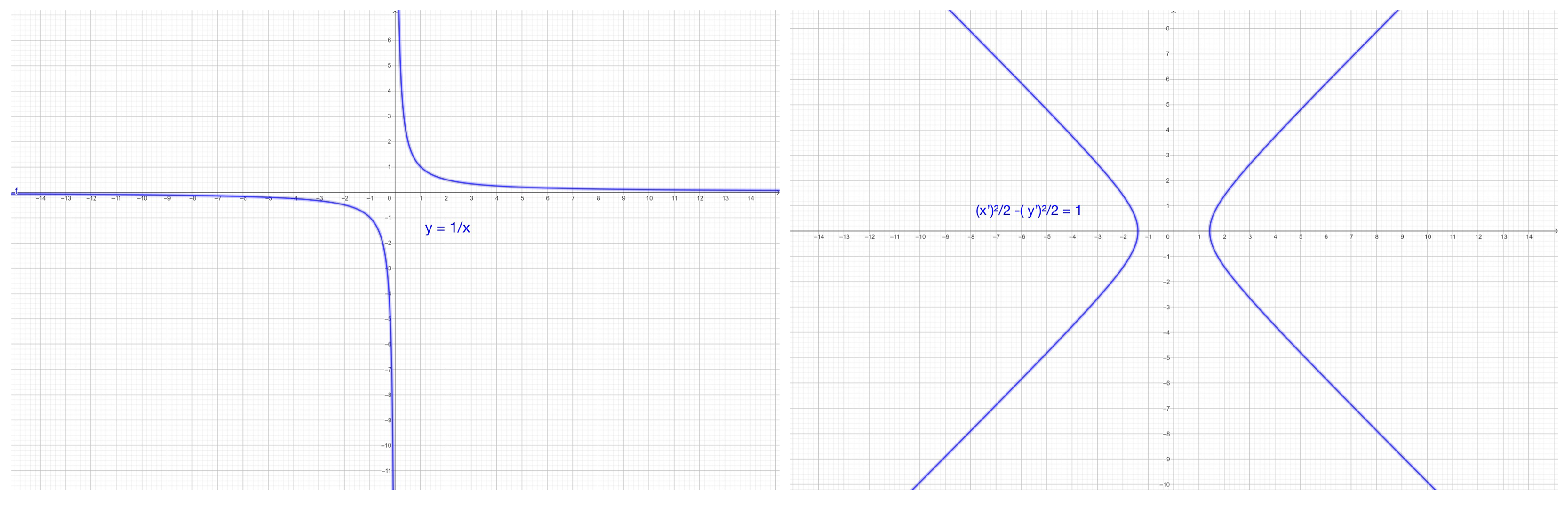
- If , the lines intersect at , and the plot is symmetric with respect to and , with . These lines are the asymptotes of two infinite families of concentric hyperbolas centered at , with one family having a vertical focal axis and the other having a horizontal focal axis.
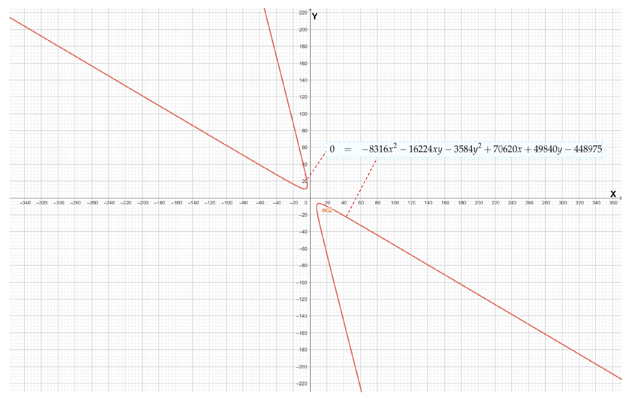
4.3. Some Curious Cases
5. The Instant Simplification of the General Conic Equation Under Rotations and Translations
6. General Features of the Conic Sections
6.1. Eccentricity
6.2. Taxonomy of the Conic Sections in
- (i) .
- (ii) .
- (iii) If , then .
- (ii) If , then . Thus, .
- (iii) If , then (ii) implies , which guarantees and ; hence, . On the other hand, if , then (ii) implies , which guarantees and ; hence, . Therefore, (i) guarantees . □
- Different among them if and only if or ,
- The same one if and only if or ,
- Two different “imaginary” straight lines if and only if or .
- Different among them if and only if and ,
- The same one if and only if ,
- Two different “imaginary” straight lines if and only if and . (Observe that, in this case, the respective independent terms are the complex numbers and , which are conjugate to each other. Indeed, and are the complex roots of the quadratic equation due to and , so .)
- (E) Cases (xiv) and (xv) are immediate consequences of Corollary 3(iii) and Theorem 4(i). □
7. Concluding Remarks
7.1. On the Relevance of Theorem 3
7.2. On the Results of This Document
- Rotational invariants (Corollary 2).
- The discriminant criterion (Corollary 3).
- Theorem 2, a more precise reformulation of the rotation angle via the conic radical.
- An improved generalization of Ayoub’s formula (Theorem 5), showing its validity for all non-degenerate conics and clarifying the role of .
- A detailed taxonomy of all possible conic loci (Theorem 6).
- Faster criteria for identifying non-graphable conics (Corollary 5 and Remark 2).
- The novel results include the following:
- The definition and properties of the conic radical ((12) and Proposition 1).
- Theorem 4, which instantaneously eliminates both rotation and translation in all real conic loci different from the degenerate parabolic cases.
- New and easier-to-apply criteria for identifying degenerate and non-degenerate parabolas without computing (Lemma 1, Corollary 4, and Remark 3).
- Finally, this work highlights the “conic radical” (12)—previously overlooked—as a central invariant, essential for formulating Theorem 3 and joining the classical conic indicators (conic discriminant, conic determinant, eccentricity, and rotation angle).
Author Contributions
Funding
Data Availability Statement
Acknowledgments
Conflicts of Interest
References
- Kindle, J.H. Theory and Problems of Plane and Solid Analytic Geometry; Schaum’s Publishing: New York, NY, USA, 1950. [Google Scholar]
- Lehmann, C.H. Analytic Geometry; John Wiley and Sons, Incorporated: New York, NY, USA, 1942. [Google Scholar]
- Oakley, C.O. An Outline of Analytic Geometry; Barnes and Noble: New York, NY, USA, 1963. [Google Scholar]
- Murdoch, D.C. Analytic Geometry with an Introduction to Vectors and Matrices; John Wiley and Sons: New York, NY, USA, 1967. [Google Scholar]
- Ramírez Galarza, A.I. Geometría Analítica. Una Introducción a la Geometría; La prensa de las Ciencias: México City, Mexico, 2013. [Google Scholar]
- Ramírez Galarza, A.I.; Seade, J. Introduction to Classical Geometries; Birkhäuser: Basel, Switzerland, 2007. [Google Scholar]
- Swokowski, E.W.; Cole, J.A. Algebra and Trigonometry with Analytic Geometry; Brooks Cole: Pacific Grove, CA, USA, 2006. [Google Scholar]
- Earl, R.; Nicholson, J. The Concise Oxford Dictionary of Mathematics; Oxford University Press: Oxford, UK, 2021. [Google Scholar]
- Brannan, D.A.; Esplen, M.F.; Gray, J.J. Geometry; Cambridge University Press: Cambridge, UK, 1999. [Google Scholar]
- Riddle, D.F. Analytic Geometry; PWS Publishing Company: Kent, WA, USA, 1996. [Google Scholar]
- Steen, F.H.; Ballou, D.H. Analytic Geometry; Ginn and Co.: Boston, MA, USA, 1955. [Google Scholar]
- Rees, P.K. Analytic Geometry; Prentice-Hall: Hoboken, NJ, USA, 1970. [Google Scholar]
- Hoffman, K.; Kunze, R. Linear Algebra; Pearson: London, UK, 1971. [Google Scholar]
- Ayoub, A.B. The Eccentricity of a Conic Section. Coll. Math. J. 2003, 34, 116–121. [Google Scholar] [CrossRef]
- Lawrence, J.D. A Catalog of Special Plane Curves; Dover Publications, Inc.: Mineola, NY, USA, 1972. [Google Scholar]
- Spain, B. Analytical Conics; Dover Publications, Inc.: Mineola, NY, USA, 2007. [Google Scholar]


Disclaimer/Publisher’s Note: The statements, opinions and data contained in all publications are solely those of the individual author(s) and contributor(s) and not of MDPI and/or the editor(s). MDPI and/or the editor(s) disclaim responsibility for any injury to people or property resulting from any ideas, methods, instructions or products referred to in the content. |
© 2025 by the authors. Licensee MDPI, Basel, Switzerland. This article is an open access article distributed under the terms and conditions of the Creative Commons Attribution (CC BY) license (https://creativecommons.org/licenses/by/4.0/).
Share and Cite
Chávez-Pichardo, M.; López-Barrientos, J.D.; Perea-Flores, S. Scrutinizing the General Conic Equation. Mathematics 2025, 13, 1428. https://doi.org/10.3390/math13091428
Chávez-Pichardo M, López-Barrientos JD, Perea-Flores S. Scrutinizing the General Conic Equation. Mathematics. 2025; 13(9):1428. https://doi.org/10.3390/math13091428
Chicago/Turabian StyleChávez-Pichardo, Mauricio, José Daniel López-Barrientos, and Saúl Perea-Flores. 2025. "Scrutinizing the General Conic Equation" Mathematics 13, no. 9: 1428. https://doi.org/10.3390/math13091428
APA StyleChávez-Pichardo, M., López-Barrientos, J. D., & Perea-Flores, S. (2025). Scrutinizing the General Conic Equation. Mathematics, 13(9), 1428. https://doi.org/10.3390/math13091428