Power Length-Biased New XLindley Distribution: Properties and Modeling of Real Data

Abstract

The increasing complexity of modern lifetime data necessitates the development of more flexible probability models. To address this need, we propose the power length-biased new XLindley (PLNXL) distribution, a novel two-parameter model tailored to model a wide range of lifetime datasets. Characterized by both shape and scale parameters, the PLNXL distribution effectively captures diverse hazard rate functions, including increasing, decreasing, and inverted bathtub-shaped forms. Additionally, its mean residual life function is capable of exhibiting decreasing, increasing, and bathtub-shaped behaviors, thereby enhancing its practical relevance. We derive key mathematical properties of the distribution, including moments, reliability measures, and entropy. The parameters are estimated using the maximum likelihood method, and simulation studies confirm the consistency and efficiency of the estimators. The applicability of the proposed model is illustrated using real-world datasets, where it consistently outperforms the existing models. These results highlight the robustness and adaptability of the PLNXL distribution for lifetime data analysis across a wide array of applications.

1. Introduction

The Weibull and gamma distributions are widely used for modeling lifetime data with monotonic hazard rates. However, they often fail to adequately capture non-monotonic failure behaviors, such as the inverted bathtub (IBT) hazard rates frequently encountered in reliability and biological studies.

Extensive mortality research has revealed a recurring trend: mortality rates start low, peak at a certain point, and then gradually decline. This distinctive pattern led to the introduction of the IBT-shaped hazard rate concept, which is now widely recognized. These hazard rates have numerous practical applications, particularly in survival analysis. They are often observed in disease progression, where mortality initially rises, reaches a peak, and then gradually decreases. Several studies have documented IBT-shaped hazard rates in various datasets. For example, Bennett [1] identified an IBT-shaped hazard rate while analyzing lung cancer data. Similarly, Efron [2] observed an increase, peak, and subsequent decline in failure rates when examining head and neck cancer cases. Furthermore, Langlands et al. [3] reported that 3878 breast cancer cases recorded in Edinburgh between 1954 and 1964 exhibited an IBT-shaped hazard function.

Compared to the more prevalent increasing failure-rate distributions, IBT distributions—those capable of exhibiting IBT-shaped hazard rates—are relatively limited. Nonetheless, they often provide superior modeling performance in specific contexts. For instance, Aalen and Gjessing [4] demonstrated that IBT distributions effectively model absorption times in Wiener processes. Likewise, Bae et al. [5] emphasized the necessity of IBT distributions for accurately representing certain degradation trajectories. Crowder et al. [6] further suggested that IBT distributions best fit datasets involving ball-bearing failure times. According to Lai and Xie [7], IBT distributions are particularly useful for modeling failure times driven by fatigue or corrosion.

Although the gamma and Weibull distributions do not exhibit an IBT-shaped hazard rate, their inverse counterparts—the inverse gamma and inverse Weibull distributions—can display such a pattern. Many inverse probability distributions exhibit the IBT structure in their hazard rates but are limited to this specific shape. For instance, the inverse gamma distribution is suitable only for modeling IBT-shaped hazard rates and cannot accommodate monotonic hazard rate patterns.

The power Lindley and weighted Lindley distributions, two-parameter extensions of the Lindley distribution [8], have recently gained popularity for the analysis of lifetime data. Although they can accommodate non-monotonic hazard rates, the power Lindley and weighted Lindley distributions are unable to exhibit the IBT-shaped hazard rate. Furthermore, both the weighted Lindley and power Lindley distributions lack a scale parameter and include only shape parameters.

Due to the significance of the Lindley distribution, many authors have modified it using different approaches and applied it for various purposes. Benchiha and Al-Omari [9] suggested generalized quasi Lindley distribution. Irshad et al. [10] introduced extended Farlie–Gumbel–Morgenstern bivariate Lindley distribution. Benchiha et al. [11] proposed the weighted generalized quasi Lindley distribution. Recently, Chouia and Zeghdoudi [12] introduced the XLindley distribution. Khodja et al. [13] introduced the new XLindley distribution. The probability density function (PDF) of the new XLindley distribution with parameter $\beta$ is given by

$$f_N\left(x\right)={\displaystyle \frac{\beta }{2}}(1+\beta x)e^{-\beta x},\beta >0,x>0,$$

with mean, survival function, and hazard rate function (HRF), respectively, given by

$$E\left(X\right)={\displaystyle \frac{2}{3\beta }},S_N\left(x\right)=\left(1+{\displaystyle \frac{1}{2}}\beta x\right)e^{-\beta x},\mathrm{and}{h}_N\left(x\right)={\displaystyle \frac{\beta +{\beta }^{2}x}{\beta x+2}}.$$

Metiri et al. [14] focused on the characterization of the XLindley distribution through its truncated moments, examined its properties, and explored its potential applications. Zinhom et al. [15] suggested the wrapped XLindley distribution. Etaga et al. [16] proposed the double XLindley distribution. Beghriche et al. [17] suggested the inverse XLindley distribution. MirMostafaee [18] introduced the exponentiated new XLindley distribution, which can be effectively used to model increasing and bathtub-shaped failure rates. Gemeay et al. [19] suggested the power new XLindley distribution. Alghamdi et al. [20] introduced the discrete Poisson quasi-XLindley distribution, highlighting its mathematical properties, formulating a regression model, and performing data analysis. Alomair et al. [21] introduced the exponentiated XLindley distribution by adding a new shape parameter to the XLindley distribution to enhance its flexibility. Musekwa and Makubate [22] proposed the exponentiated generalized XLindley distribution, a three-parameter model with a versatile PDF that can be positively or negatively skewed, reverse-J shaped, or symmetric. Using the alpha power transformation technique, Alsadat [23] introduced the truncated new XLindley distribution. The truncated forms of the new XLindley distribution are introduced and studied by Kouadria and Zeghdoudi [24].

Numerous fields, including engineering, biology, ecology, branching processes, and reliability, use weighted probability distributions. Rao [25] considered weighted distribution to model the statistical data for which standard distributions are not appropriate. ul Haq et al. [26] introduced the Marshall–Olkin length-biased exponential distribution. Rajagopalan et al. [27] proposed the length-biased Aradhana distribution. Hassan et al. [28] studied the weighted power Lomax distribution and its length biased version. Chaito and Khamkong [29] studied the length-biased Weibull–Rayleigh distribution for application to hydrological data. Alzoubi [30] suggested the length-biased Loai distribution.

For a random variable Y with PDF $f_0\left(y\right)$ and a non-negative weight function w, the PDF of the corresponding weighted distribution is given by

$$g\left(y\right)={\displaystyle \frac{w\left(y\right)f_0\left(y\right)}{E\left(w\right(Y\left)\right)}},$$

where $E\left(w\right(Y\left)\right)$ is the expectation of $w\left(Y\right)$. If $w\left(y\right)=y^c,c>0$, the resulting weighted distribution is called a size-biased distribution. A size-biased distribution with $c=1$ is called a length-biased distribution. Thus, the PDF of length-biased distribution is

$$g\left(y\right)={\displaystyle \frac{y{f}_0\left(y\right)}{E\left(Y\right)}}.$$

Hence, the length-biased new XLindley distribution has the PDF given by

$$g_0\left(y\right)={\displaystyle \frac{1}{3}}{\beta }^{2}y{e}^{-\beta y}(\beta y+1),y>0,\beta >0.$$

(1)

The objectives of the present study are outlined as follows:

• Introduce the power length-biased new XLindley distribution as a novel probability model for lifetime data.
• Explore and validate the statistical properties of the proposed distribution and demonstrate its suitability for modeling datasets with increasing, decreasing, and inverted bathtub-shaped hazard rates.
• Estimate the parameters of the proposed distribution using the maximum likelihood estimation (MLE) method and assess the efficiency of the MLE estimators through simulated observations.
• Illustrate the applicability of the proposed distribution by fitting it to real datasets in comparison with existing competing models and demonstrate its superior fit.

The proposed two-parameter probability model offers a high degree of flexibility while maintaining mathematical simplicity. Despite having a single shape parameter and a single scale parameter, the model effectively captures decreasing, increasing, and IBT hazard rates. This adaptability represents a significant advantage over traditional models such as the Weibull and gamma distributions, which require additional modifications or extra parameters to accommodate such behaviors. The ability to model non-monotonic hazard rates with just two parameters enhances the proposed distribution’s efficiency in real-world applications, minimizing the need for complex estimation procedures while still achieving superior goodness of fit. Many existing flexible lifetime models introduce additional shape parameters, increasing computational complexity and making parameter estimation more challenging. In contrast, the proposed model retains its mathematical tractability while remaining versatile enough to describe complex failure behaviors. Moreover, the model’s reliability function is expressed in a closed form, facilitating practical applications in predictive maintenance, risk assessment, and decision making. This simplicity enhances its applicability in real-world reliability studies, industrial quality control, and healthcare research, where both interpretability and computational efficiency are essential. Consequently, the proposed model serves as a valuable contribution to probability and reliability theory, expanding the range of available tools for modeling lifetime data across various disciplines.

The structure of the paper is organized as follows: Section 2 introduces the PLNXL distribution and examines its statistical properties. In Section 3, the parameters of the PLNXL distribution are estimated using the maximum likelihood estimation technique. Section 4 presents a method for generating random observations along with a simulation study. Section 5 applies the PLNXL distribution and other competing models to analyze real-world datasets. The paper concludes in the final section.

2. PLNXL Distribution and Its Properties

In this section, the PLNXL distribution is introduced along with some of its statistical properties, including reliability analysis, raw moments, and entropy.

2.1. The PLNXL and Its Shape

The PDF of the PLNXL distribution is given by

$$f\left(x\right)={\displaystyle \frac{\alpha {\beta }^2}{3}}{x}^{2\alpha -1}\left(1+\beta x^{\alpha }\right)e^{-\beta x^{\alpha }},x>0,\alpha >0,\beta >0.$$

(2)

Here, $\alpha$ and $\beta$ are shape and scale parameters, respectively. The PDF in (2) is obtained by taking the power transformation $Y^{1/\alpha }$, where Y denotes a length-biased new XLindley random variable with the PDF (1). The PDF in (2) can also be represented as a mixture of PDFs of generalized gamma (GG) distributions. To support this claim, we recall that the PDF of the GG distribution with shape parameters $\theta$ and $\alpha$ and a scale parameter $\beta$ is given by

$$f_{GG}\left(x\right)={\displaystyle \frac{\alpha {\beta }^{\theta }}{\mathrm{\Gamma }\left(\theta \right)}}{x}^{\alpha \theta -1}{e}^{-\beta x^{\alpha }},\alpha >0,\beta >0,\theta >0,x>0,$$

where $\mathrm{\Gamma }\left(x\right)={\int }_0^{\infty }{e}^{-y}{y}^{x-1}dy$ denotes the gamma function. The PDF in (2) can be represented as

$$f\left(x\right)=p{f}_1\left(x\right)+(1-p)f_2\left(x\right),$$

where $f_1(·)$ is the PDF of the GG distribution with shape parameters 2 and $\alpha$ and a scale parameter $\beta$; $f_2(·)$ is the PDF of the GG distribution with shape parameters 3 and $\alpha$ and a scale parameter $\beta$; and the mixing proportion $p={\displaystyle \frac{1}{3}}$.

The shape features of the PDF of the PLNXL distribution with respect to the values of the parameters $\alpha$ and $\beta$ will next be discussed.

Theorem 1.

The PDF in Equation (2) is either

(i) 

decreasing if $\alpha \le {\displaystyle \frac{1}{2}}$;

(ii) 

unimodal if $\alpha >{\displaystyle \frac{1}{2}}$.

Proof is provided in Appendix A.

The PDF plots of the PLNXL distribution for chosen values of the parameters ($\alpha =0.9$, $\beta =$ 0.2, 0.25, 0.3, 0.35, 0.4), ($\alpha =2$, $\beta =$0.2, 0.25, 0.3, 0.35, 0.4), ($\beta =0.09$, $\alpha =1.5,2.4,3.3,3.8,4.3$), ($\alpha =0.5$, $\beta =1$), ($\alpha =0.5$, $\beta =7$), and ($\alpha =0.5$, $\beta =3$) are displayed in Figure 1, which also illustrates all of the forms outlined in Theorem 1, as decreasing and increasing–decreasing.

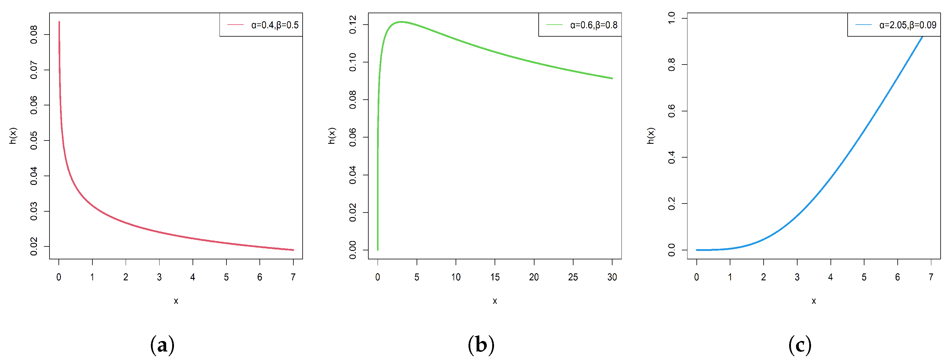
2.2. Reliability Analysis

Apart from the PDF, other functions should also be given specific consideration for a better understanding of the distribution. In particular, the distribution and survival functions of the PLNXL distribution are as follows:

$$F\left(x\right)=1-{\displaystyle \frac{{\beta }^2{x}^{2\alpha }+3\beta x^{\alpha }+3}{3}}{e}^{-\beta x^{\alpha }},x>0,$$

and

$$S\left(x\right)={\displaystyle \frac{{\beta }^2{x}^{2\alpha }+3\beta x^{\alpha }+3}{3}}{e}^{-\beta x^{\alpha }},x>0.$$

Note that the PLNXL distribution has a closed-form expression for distribution and survival functions. Next, we consider the hazard rate function (HRF) and its various shapes.

The HRF is given by

$$h\left(x\right)={\displaystyle \frac{\alpha {\beta }^2}{{\beta }^2{x}^{2\alpha }+3\beta x^{\alpha }+3}}(1+\beta x^{\alpha })x^{2\alpha -1},x>0.$$

(3)

In the following theorem, we discuss various shapes of HRF of PLNXL distribution.

Theorem 2.

The hazard rate function in Equation (3) is:

(i) 

increasing if $\alpha \ge 1$;

(ii) 

decreasing if $\alpha \le {\displaystyle \frac{1}{2}}$;

(iii) 

IBT-shaped if ${\displaystyle \frac{1}{2}}<\alpha <1$.

Proof is provided in Appendix A.

The shape characteristics of the HRF are displayed in Figure 2 for several values of the parameters. Figure 2 reveals that the distribution possesses various shapes, including decreasing, increasing–decreasing, and increasing forms, making it more flexible for fitting different types of data.

The mean residual life function (MRLF) is a crucial aspect of any lifetime distribution in addition to the HRF. The MRLF of PLNXL is

$$\begin{array}{ccc}\hfill \mu \left(x\right)& =& {\displaystyle \frac{1}{S\left(x\right)}}{\int }_x^{\infty }tf\left(t\right)dt-x\hfill \\ & =& {\displaystyle \frac{e^{\beta x^{\alpha }}}{{\beta }^{1/\alpha }\left({\beta }^2{x}^{2\alpha }+3\beta x^{\alpha }+3\right)}}\left(\mathrm{\Gamma }\left({\displaystyle \frac{2\alpha +1}{\alpha }},\beta x^{\alpha }\right)+\mathrm{\Gamma }\left({\displaystyle \frac{3\alpha +1}{\alpha }},\beta x^{\alpha }\right)\right)-x.\hfill \end{array}$$

Next, we discuss the shape of MRLF in the following theorem.

Theorem 3.

The mean residual life function $\mu \left(x\right)$ of the PLNXL is

(i) 

increasing if $\alpha \le {\displaystyle \frac{1}{2}}$;

(ii) 

decreasing if $\alpha \ge 1$;

(iii) 

bathtub-shaped if ${\displaystyle \frac{1}{2}}<\alpha <1$.

The MRLF is increasing (decreasing) if the corresponding HRF is decreasing (increasing) [31]. Hence, MRLF of PLNXL is increasing (decreasing) if $\alpha \le {\displaystyle \frac{1}{2}}$ ($\alpha \ge 1$).

Furthermore, if HRF $h\left(x\right)$ has a bathtub (IBT) shape, then MRLF $\mu \left(x\right)$ has an IBT (bathtub) shape, provided $h\left(0\right)\mu \left(0\right)>1$ ($\le 1$) [32]. Hence, the proof.

The shape characteristics of the MRLF are displayed in Figure 3 for several values of the parameters. It is clear that the MRLF of the PLNXL distribution exhibits decreasing–increasing, increasing, and decreasing patterns.

The scale parameter influences the dispersion and spread of the distribution, allowing it to adjust to different data ranges. The shape parameter plays a crucial role in controlling the overall behavior of the PDF and HRF, enabling the model to capture a wide variety of distributional forms. By appropriately selecting these parameters, the model can exhibit both decreasing and unimodal density shapes, as well as failure rates that are decreasing, increasing, or inverted bathtub shaped, making it more versatile than many traditional distributions. These properties enhance the model’s applicability to diverse real-world scenarios, particularly in reliability and survival analysis.

2.3. The Raw Moments

Finding the raw moment of a random variable is essential because it gives us insight into the behavior of the distribution, including its variability and central tendencies. They make it possible to compute crucial statistics, including the variance and mean, which are necessary for making wise choices in a variety of domains. In this section, we establish some intriguing closed-form moment features of the PLNXL distribution.

The rth raw moment of the PLNXL distribution is

$$E\left(X^r\right)={\mu }_r^{\prime }={\displaystyle \frac{\mathrm{\Gamma }\left(2+\frac{r}{\alpha }\right)(r+3\alpha )}{3\alpha {\beta }^{r/\alpha }}}.$$

(4)

Using Equation (4), the first four raw moments about the origin are given as follows:

$${\mu }_1^{\prime }={\displaystyle \frac{\mathrm{\Gamma }\left(\frac{2\alpha +1}{\alpha }\right)(3\alpha +1)}{3\alpha {\beta }^{1/\alpha }}},{\mu }_2^{\prime }={\displaystyle \frac{\mathrm{\Gamma }\left(\frac{2\alpha +2}{\alpha }\right)(3\alpha +2)}{3\alpha {\beta }^{2/\alpha }}},$$

$${\mu }_3^{\prime }={\displaystyle \frac{\mathrm{\Gamma }\left(\frac{2\alpha +3}{\alpha }\right)(3\alpha +3)}{3\alpha {\beta }^{3/\alpha }}},\mathrm{and}{\mu }_4^{\prime }={\displaystyle \frac{\mathrm{\Gamma }\left(\frac{2\alpha +4}{\alpha }\right)(3\alpha +4)}{3\alpha {\beta }^{4/\alpha }}}.$$

Hence, the expected value and variance of PLNXL are obtained by

$$E\left(X\right)=\mu ={\displaystyle \frac{\mathrm{\Gamma }\left(\frac{2\alpha +1}{\alpha }\right)(3\alpha +1)}{3\alpha {\beta }^{1/\alpha }}},$$

and

$$V\left(X\right)={\sigma }^2={\displaystyle \frac{\mathrm{\Gamma }\left(\frac{2\alpha +2}{\alpha }\right)(3\alpha +2)}{3\alpha {\beta }^{2/\alpha }}}-{\left({\displaystyle \frac{\mathrm{\Gamma }\left(\frac{2\alpha +1}{\alpha }\right)(3\alpha +1)}{3\alpha {\beta }^{1/\alpha }}}\right)}^2.$$

2.4. Entropy

Entropy is a crucial measure in lifetime probability models as it quantifies the uncertainty and randomness associated with the distribution of lifetimes. Researchers consider entropy to assess the unpredictability of failure times, compare different models, and optimize parameter estimation. In practical applications, entropy plays a vital role in reliability engineering by helping design maintenance strategies in survival analysis for predicting patient outcomes and in actuarial science for assessing financial risks. It is also valuable in stress–strength analysis, where it quantifies uncertainty in system durability under varying conditions. By incorporating entropy into lifetime models, researchers can enhance their understanding of uncertainty, improve model selection, and develop more robust statistical methods for real-world application.

For a continuous random variable X with a PDF $f\left(x\right)$ given in Equation (2), the Rényi entropy [33] is defined as

$$H_{\eta }\left(X\right)={\displaystyle \frac{1}{1-\eta }}log\left({\int }_{-\infty }^{\infty }{\left[f\left(x\right)\right]}^{\eta }dx\right)={\displaystyle \frac{1}{1-\eta }}log\left({\displaystyle \frac{\mathbf{Q}{\left(\frac{\alpha {\beta }^2}{3}\right)}^{\eta }}{\alpha }}\right),\eta >0,\eta \ne 1,$$

$$\begin{array}{cc}\hfill \mathbf{Q}& =\pi {\beta }^{-2\eta }csc\left({\displaystyle \frac{\pi \left(\right(3\alpha -1)\eta +1)}{\alpha }}\right)\times \left({\beta }^{3\eta }{\left(\beta \eta \right)}^{{\displaystyle \frac{-3\alpha \eta +\eta -1}{\alpha }}}{}_1\tilde{F}_1\left(-\eta ;{\displaystyle \frac{-3\eta \alpha +\alpha +\eta -1}{\alpha }};\eta \right)\right.\hfill \\ \hfill & \left.-{\displaystyle \frac{{\beta }^{\frac{\eta -1}{\alpha }}\mathrm{\Gamma }\left(\frac{2\alpha \eta -\eta +1}{\alpha }\right){}_1\tilde{F}_1\left(\frac{2\alpha \eta -\eta +1}{\alpha };\frac{3\eta \alpha +\alpha -\eta +1}{\alpha };\eta \right)}{\mathrm{\Gamma }(-\eta )}}\right),\hfill \end{array}$$

where ${}_1\tilde{F}_1(a;b;z)={\displaystyle \frac{{}_{1}F_1(a;b;z)}{\mathrm{\Gamma }\left(b\right)}}$ is the regularized confluent hypergeometric function of the first kind, and Kummer’s function ${}_{1}F_1(a;b;z)$ is defined as

$${}_{1}F_1(a;b;z)=\sum _{n=0}^{\infty }{\displaystyle \frac{{\left(a\right)}_n}{{\left(b\right)}_n}}{\displaystyle \frac{z^n}{n!}},{\left(q\right)}_n=\left\{\begin{array}{cc}1\hfill & \mathrm{if}n=0\hfill \\ q(q+1)\cdots (q+n-1)\hfill & \mathrm{if}n>0.\hfill \end{array}\right.$$

Tsallis [34] suggested Tsallis Entropy and defined this measure as

$$H_{\gamma }\left(X\right)={\displaystyle \frac{1}{\gamma -1}}\left(1-\underset{-\infty }{\overset{\infty }{\int }}{f}^{\gamma }\left(x\right)dx\right)={\displaystyle \frac{1}{\gamma -1}}\left(1-{\displaystyle \frac{\mathrm{\Psi }{\left(\frac{\alpha {\beta }^2}{3}\right)}^{\gamma }}{\alpha }}\right),\gamma >0,\gamma \ne 1,$$

where

$$\begin{array}{cc}\hfill \mathrm{\Psi }& =\pi {\beta }^{-2\gamma }csc\left({\displaystyle \frac{\pi \left(\right(3\alpha -1)\gamma +1)}{\alpha }}\right)\times \left({\beta }^{3\gamma }{\left(\beta \gamma \right)}^{{\displaystyle \frac{-3\alpha \gamma +\gamma -1}{\alpha }}}{}_1\tilde{F}_1\left(-\gamma ;{\displaystyle \frac{-3\gamma \alpha +\alpha +\gamma -1}{\alpha }};\gamma \right)\right.\hfill \\ \hfill & \left.-{\displaystyle \frac{{\beta }^{\frac{\gamma -1}{\alpha }}\mathrm{\Gamma }\left(\frac{2\alpha \gamma -\gamma +1}{\alpha }\right){}_1\tilde{F}_1\left(\frac{2\alpha \gamma -\gamma +1}{\alpha };\frac{3\gamma \alpha +\alpha -\gamma +1}{\alpha };\gamma \right)}{\mathrm{\Gamma }(-\gamma )}}\right).\hfill \end{array}$$

In the next section, we discuss the estimation of model parameters.

3. Model Parameter Estimation

Various estimation techniques exist in the statistical literature for parametric estimation. Several studies have explored different statistical approaches for parameter estimation. Kızılaslan [35] applied classical and Bayesian estimation techniques to assess reliability in a multicomponent stress–strength model under the proportional reversed hazard rate framework. Agiwal [36] utilized both MLE and Bayesian approaches to estimate stress–strength reliability using the inverse Chen distribution for failure time data. Furthermore, Xu et al. [37] proposed an expectation–maximization (EM) algorithm for parameter estimation in a multivariate Student-t process model designed for dependent tail-weighted degradation data. They also developed a bootstrap-based method for interval estimation, enhancing the robustness of the parameter inference process. Zhuang et al. [38] employed both the maximum likelihood estimation (MLE) and Bayesian methods to estimate the unknown parameters of a two-phase degradation model based on a reparameterized inverse Gaussian process.

The parameters of the model are estimated using the maximum likelihood (ML) method. We construct the asymptotic confidence interval (CI) of the parameters using these estimators. The decision to use the ML method for parameter estimation was driven by several factors that align with the nature of the model and the goals of the analysis. ML estimation is straightforward to implement, especially in cases where the likelihood function is tractable and differentiable. Given that our model has well-defined likelihood functions, the ML method allows for efficient optimization without the complexity of integrating over the posterior distribution, as is required in Bayesian approaches. Under regular conditions, the ML estimators are consistent and asymptotically efficient. This makes ML an attractive choice when large sample sizes are available, as it leads to highly reliable estimates. In situations where the sample size is moderate and prior information is either unavailable or unreliable, the Bayesian approach can be highly sensitive to the choice of priors. In contrast, the ML method is non-informative in this regard, and its estimation does not rely on the subjective specification of priors, making it more robust in such settings.

3.1. ML Estimation

Now, let us describe the ML method in our exact setting. Given the random sample $x_1,x_2,\dots ,x_n$ from a random variable X with the PLNXL distribution, the maximum likelihood estimates (MLEs) of parameters $\alpha$ and $\beta$ are obtained by maximizing the likelihood function L, which is given by

$$L=L(\alpha ,\beta )=\prod _{i=1}^{n}f\left(x_i\right)=\prod _{i=1}^n{\displaystyle \frac{\alpha {\beta }^2}{3}}{e}^{-\beta x_i^{\alpha }}(1+\beta x_i^{\alpha })x_i^{2\alpha -1}.$$

The logarithm of this equation is given as

$$log\left(L\right)=nlog\left({\displaystyle \frac{\alpha {\beta }^2}{3}}\right)-\beta \sum _{i=1}^n{x}_i^{\alpha }+\sum _{i=1}^{n}log(1+\beta x_i^{\alpha })+(2\alpha -1)\sum _{i=1}^{n}log\left(x_i\right).$$

The MLEs of parameters $\alpha$ and $\beta$ can be obtained by solving the non-linear Equations (5) and (6), given by

$${\displaystyle \frac{\partial log\left(L\right)}{\partial \alpha }}=0\Rightarrow {\displaystyle \frac{n}{\alpha }}-\beta \sum _{i=1}^n{x}_i^{\alpha }log\left(x_i\right)+\sum _{i=1}^n{\displaystyle \frac{\beta x_i^{\alpha }log\left(x_i\right)}{1+\beta x_i^{\alpha }}}+2\sum _{i=1}^{n}log\left(x_i\right)=0,$$

and

$${\displaystyle \frac{\partial log\left(L\right)}{\partial \beta }}=0\Rightarrow {\displaystyle \frac{2n}{\beta }}+\sum _{i=1}^n{\displaystyle \frac{x_i^{\alpha }}{1+\beta x_i^{\alpha }}}-\sum _{i=1}^n{x}_i^{\alpha }=0.$$

3.2. Asymptotic Confidence Interval

To obtain the asymptotic confidence interval (CI), we make use of the following integrals, as provided by [39]:

$${\int }_0^{\infty }{t}^{v-1}log\left(t\right)e^{-\beta t}dt={\displaystyle \frac{\mathrm{\Gamma }\left(v\right)}{{\beta }^v}}[\psi \left(v\right)-log\left(\beta \right)],v,\beta >0,$$

and

$${\int }_0^{\infty }{t}^{v-1}{(log\left(t\right))}^2{e}^{-\beta t}dt={\displaystyle \frac{\mathrm{\Gamma }\left(v\right)}{{\beta }^v}}\left({[\psi \left(v\right)-log\left(\beta \right)]}^2+\zeta (2,v)\right),v,\beta >0,$$

where $\psi \left(t\right)={\displaystyle \frac{d}{dt}}log\left(\mathrm{\Gamma }\left(t\right)\right)$ and $\zeta (z,v)$ denote the digamma function and Riemann’s zeta function, respectively. The Riemann’s zeta function is given by

$$\zeta (z,v)=\sum _{m=0}^{\infty }{\displaystyle \frac{1}{{(v+m)}^z}},z>1,v\ne 0,-1,-2,\dots$$

The above expressions are used to compute the following expectations for a random variable X that follows the PLNXL distribution:

$$\begin{array}{cc}\hfill E\left[X^{\alpha }log\left(X\right)\right]& ={\displaystyle \frac{1}{{\beta }^2}}(\psi \left(2\right)+2\psi \left(3\right)-3log\left(\beta \right)),\hfill \\ \hfill E\left[X^{\alpha }{(log\left(X\right))}^2\right]& ={\displaystyle \frac{1}{3{\alpha }^2\beta }}\left(2\left({(\psi \left(3\right)-log\left(\beta \right))}^2+\zeta (2,3)\right)+6\left({(\psi \left(4\right)-log\left(\beta \right))}^2+\zeta (2,4)\right)\right),\hfill \\ \hfill E\left[{\displaystyle \frac{X^{\alpha }{(log\left(X\right))}^2}{{(1+\beta X^{\alpha })}^2}}\right]& ={\displaystyle \frac{{\beta }^2}{3{\alpha }^2}}{\int }_0^{\infty }{\displaystyle \frac{t^2{(log\left(t\right))}^2{e}^{-\beta t}}{(1+\beta t)}}dt={\displaystyle \frac{2}{3{\alpha }^2\beta }}\left[{(log\beta )}^2-2(log\beta )+2\right].\hfill \end{array}$$

On the basis of a single observation, the expected Fisher information matrix of $\theta =(\alpha ,\beta )$ is given by

$$I\left(\theta \right)=\left[I_{ij}\right]=\underset{m,n\to \infty }{lim}E\left[-{\displaystyle \frac{{\partial }^2}{\partial {\theta }_i\partial {\theta }_j}}logf\left(x\right)\right],$$

where

$$\begin{array}{cc}\hfill I_{11}& ={\displaystyle \frac{1}{{\alpha }^2}}+\beta E\left[X^{\alpha }{(log\left(X\right))}^2\right]-\beta E\left[{\displaystyle \frac{X^{\alpha }{(log\left(X\right))}^2}{{(1+\beta X^{\alpha })}^2}}\right]\hfill \\ \hfill & ={\displaystyle \frac{1}{{\alpha }^2}}+{\displaystyle \frac{1}{3{\alpha }^2\beta }}\left(2\left({(\psi \left(3\right)-log\left(\beta \right))}^2+\zeta (2,3)\right)+6\left({(\psi \left(4\right)-log\left(\beta \right))}^2+\zeta (2,4)\right)\right)\hfill \\ & -{\displaystyle \frac{{\beta }^3}{3{\alpha }^2}}{\int }_0^{\infty }{\displaystyle \frac{t^2{(log\left(t\right))}^2{e}^{-\beta t}}{(1+\beta t)}}dt\hfill \\ \hfill & ={\displaystyle \frac{1}{{\alpha }^2}}+{\displaystyle \frac{1}{3{\alpha }^2\beta }}\left(2\left({(\psi \left(3\right)-log\left(\beta \right))}^2+\zeta (2,3)\right)+6\left({(\psi \left(4\right)-log\left(\beta \right))}^2+\zeta (2,4)\right)\right)\hfill \\ & -{\displaystyle \frac{2}{3{\alpha }^2}}\left[{(log\beta )}^2-2(log\beta )+2\right],\hfill \end{array}$$

$$\begin{array}{cc}\hfill I_{22}& ={\displaystyle \frac{2}{{\beta }^2}}+E\left({\displaystyle \frac{X^{2\alpha }}{{(1+\beta X^{\alpha })}^2}}\right)={\displaystyle \frac{2}{{\beta }^2}}+{\displaystyle \frac{{\beta }^2}{3}}{\int }_0^{\infty }{\displaystyle \frac{t^3}{1+\beta t}}{e}^{-\beta t}dt,\hfill \end{array}$$

$$\begin{array}{cc}\hfill I_{12}& =E\left[X^{\alpha }log\left(X\right)\right]-E\left[{\displaystyle \frac{X^{\alpha }log\left(X\right)}{1+\beta X^{\alpha }}}\right]+{\beta }^{2}E\left[{\displaystyle \frac{X^{2\alpha }{(log\left(X\right))}^2}{{(1+\beta X^{\alpha })}^2}}\right]\hfill \\ \hfill & ={\displaystyle \frac{1}{{\beta }^2}}(\psi \left(2\right)+2\psi \left(3\right)-3log\left(\beta \right))-{\displaystyle \frac{{\beta }^2}{3\alpha }}{\int }_0^{\infty }{t}^{2}log\left(t\right)e^{-\beta t}dt+{\displaystyle \frac{{\beta }^4}{3{\alpha }^2}}{\int }_0^{\infty }{\displaystyle \frac{t^3{(log\left(t\right))}^2{e}^{-\beta t}}{(1+\beta t)}}dt\hfill \\ \hfill & ={\displaystyle \frac{1}{{\beta }^2}}(\psi \left(2\right)+2\psi \left(3\right)-3log\left(\beta \right))-{\displaystyle \frac{2}{3\alpha \beta }}\left({\displaystyle \frac{3}{2}}-log\beta \right)+{\displaystyle \frac{2}{{\alpha }^2}}\left({(log\beta )}^2-2(log\beta )+2\right).\hfill \end{array}$$

The asymptotic distribution of an MLE $\widehat{\theta }$ (Lehmann and Casella, 1998 [40]) of the unknown parameter vector $\theta =(\alpha ,\beta )$ is given by

$$\sqrt{n}(\widehat{\theta }-\theta )\stackrel{d}{\to }{N}_2(0,I^{-1}\left(\theta \right)),$$

where $\stackrel{d}{\to }$ denotes the convergence in distribution, $I^{-1}\left(\theta \right)$ is the inverse of the matrix I, and $N_2(.,.)$ denotes the bivariate normal distribution.

Hence, the asymptotic variance–covariance matrix of the MLE is given by

$${\displaystyle \frac{1}{n}}{I}^{-1}\left(\theta \right)=\left[\begin{array}{cc}\mathrm{Var}\left(\widehat{\alpha }\right)& \mathrm{Cov}(\widehat{\alpha },\widehat{\beta })\\ \mathrm{Cov}(\widehat{\alpha },\widehat{\beta })& \mathrm{Var}\left(\widehat{\beta }\right)\end{array}\right].$$

The $100(1-\delta )\%$ asymptotic CIs for parameters $\alpha$ and $\beta$ are, respectively, given by

$$(\widehat{\alpha }-z_{\delta /2}\sqrt{\widehat{\mathrm{Var}\left(\widehat{\alpha }\right)}},\widehat{\alpha }+z_{\delta /2}\sqrt{\widehat{\mathrm{Var}\left(\widehat{\alpha }\right)}}),(\widehat{\beta }-z_{\delta /2}\sqrt{\widehat{\mathrm{Var}\left(\widehat{\beta }\right)}},\widehat{\beta }+z_{\delta /2}\sqrt{\widehat{\mathrm{Var}\left(\widehat{\beta }\right)}}).$$

Since the parameters are known to be positive, the previously mentioned CI forms may result in negative lower bounds, which is problematic. The logarithmic transformation is therefore applied, and the asymptotic normality distribution of $log\left(\widehat{\alpha }\right)$ and $log\left(\widehat{\beta }\right)$ is obtained using the delta technique. Thus, we have

$$\sqrt{n}(log\left(\widehat{\alpha }\right)-log\left(\alpha \right))\stackrel{d}{\to }{N}_2\left(0,n{\displaystyle \frac{\mathrm{Var}\left(\widehat{\alpha }\right)}{{\alpha }^2}}\right),\sqrt{n}(log\left(\widehat{\beta }\right)-log\left(\beta \right))\stackrel{d}{\to }{N}_2\left(0,n{\displaystyle \frac{\mathrm{Var}\left(\widehat{\beta }\right)}{{\beta }^2}}\right).$$

Now, the asymptotic $100(1-\delta )\%$ CIs for $log\left(\alpha \right)$ and $log\left(\beta \right)$ are given by

$$\left(log\left(\widehat{\alpha }\right)-z_{\delta /2}\sqrt{{\displaystyle \frac{\widehat{\mathrm{Var}\left(\widehat{\alpha }\right)}}{\widehat{\alpha }}}},log\left(\widehat{\alpha }\right)+z_{\delta /2}\sqrt{{\displaystyle \frac{\widehat{\mathrm{Var}\left(\widehat{\alpha }\right)}}{\widehat{\alpha }}}}\right)=\left(L_1,U_1\right),$$

$$\left(log\left(\widehat{\beta }\right)-z_{\delta /2}\sqrt{{\displaystyle \frac{\widehat{\mathrm{Var}\left(\widehat{\beta }\right)}}{\widehat{\beta }}}},log\left(\widehat{\beta }\right)+z_{\delta /2}\sqrt{{\displaystyle \frac{\widehat{\mathrm{Var}\left(\widehat{\beta }\right)}}{\widehat{\beta }}}}\right)=\left(L_2,U_2\right).$$

We can raise the power of the exponential to obtain the asymptotic $100(1-\delta )\%$ CIs for $\alpha$ and $\beta$, which are, respectively, given by $\left(e^{L_1},e^{U_1}\right),\left(e^{L_2},e^{U_2}\right).$

4. Generation of Random Observations and Simulation Study

4.1. Algorithm to Generate Random Observations

To generate n random observations, say $x_1,x_2,\dots ,x_n$, we provide an algorithm based on the stochastic structure of the PLNXL distribution.

• Step 1: Generate n observations $y_i^{\prime }$ and $y_i^{″}$ from the following GG distributions: $GG(2,\alpha ,\beta )$ and $GG(3,\alpha ,\beta )$, respectively.
• Step 2: Generate n observations $u_i$ from the uniform over $(0,1)$.
• Step 3: If $u_i\le 1/3$, set $x_i=y_i^{\prime }$; else, set $x_i=y_i^{″}$.
  Simulation studies can be carried out to evaluate the effectiveness of estimating techniques, among other things, using these generated data.

4.2. A Simulation Study

Random observations are generated from the PLNXL distribution using the above procedure in order to calculate the bias, mean square error (MSE), average estimate (AE), average width (AW), and coverage probability (CP), i.e., the percentage of intervals containing the true value of 95% asymptotic CI. The following parameter combinations, $(\alpha =0.6,\beta =0.6)$, $(\alpha =3.3,\beta =0.1)$, and $(\alpha =2,\beta =1.5)$, were used in the simulation, which was run $N=10000$ times with sample sizes of $n=$ 20, 50, 100, and 150.

For the estimators $\widehat{\alpha }$ and $\widehat{\beta }$, the AE, estimated bias, and estimated MSE can be obtained by

$$\mathrm{AE}\left(\widehat{\alpha }\right)={\displaystyle \frac{1}{N}}\sum _{i=1}^N{\widehat{\alpha }}_i,\mathrm{Bias}\left(\widehat{\alpha }\right)={\displaystyle \frac{1}{N}}\sum _{i=1}^N{\widehat{\alpha }}_i-\alpha ,\mathrm{MSE}\left(\widehat{\alpha }\right)={\displaystyle \frac{1}{N}}\sum _{i=1}^N{\left({\widehat{\alpha }}_i-\alpha \right)}^2,$$

$$\mathrm{AE}\left(\widehat{\beta }\right)={\displaystyle \frac{1}{N}}\sum _{i=1}^N{\widehat{\beta }}_i,\mathrm{Bias}\left(\widehat{\beta }\right)={\displaystyle \frac{1}{N}}\sum _{i=1}^N({\widehat{\beta }}_i-\beta ),\mathrm{MSE}\left(\widehat{\beta }\right)={\displaystyle \frac{1}{N}}\sum _{i=1}^N{\left({\widehat{\beta }}_i-\beta \right)}^2.$$

Table 1. AE, bias, MSE, and AW (CP) for the parameters $\alpha$ and $\beta$.

Case	Parameters	n	AE	Bias	MSE	AW (CP)
I	$\alpha$	20	0.6449	0.0449	0.0167	0.4288 (0.9418)
	$\beta$	20	0.5749	−0.0250	0.0396	0.7295 (0.8936)
	$\alpha$	50	0.6162	0.0162	0.0048	0.2591 (0.95)
	$\beta$	50	0.5898	−0.0101	0.0153	0.4752 (0.9266)
	$\alpha$	100	0.6087	0.0087	0.0022	0.1810 (0.9514)
	$\beta$	100	0.5928	−0.0071	0.0075	0.3386 (0.9394)
	$\alpha$	150	0.6055	0.0055	0.0014	0.1470 (0.9470)
	$\beta$	150	0.5956	−0.0043	0.0050	0.2775 (0.9432)
II	$\alpha$	20	3.5332	0.2332	0.4780	2.3489 (0.9474)
	$\beta$	20	0.0982	−0.0017	0.0037	0.2259 (0.8480)
	$\alpha$	50	3.3969	0.0969	0.1519	1.4283 (0.9468)
	$\beta$	50	0.0983	−0.0016	0.0014	0.1472 (0.9018)
	$\alpha$	100	3.3487	0.0487	0.0701	0.9957 (0.9480)
	$\beta$	100	0.0990	−0.0009	0.0007	0.1056 (0.9226)
	$\alpha$	150	3.3298	0.0298	0.0424	0.8083 (0.9536)
	$\beta$	150	0.0994	−0.0005	0.0004	0.0868 (0.9364)
III	$\alpha$	20	2.1542	0.1542	0.1894	1.4322 (0.9432)
	$\beta$	20	1.4691	−0.0308	0.0952	1.1467 (0.9242)
	$\alpha$	50	2.0556	0.0556	0.0557	0.8643 (0.946)
	$\beta$	50	1.4874	−0.0125	0.0367	0.7314 (0.9396)
	$\alpha$	100	2.0279	0.0279	0.0248	0.6029 (0.9514)
	$\beta$	100	1.4965	−0.0034	0.0179	0.5189 (0.9462)
	$\alpha$	150	2.0152	0.0152	0.0162	0.4892 (0.9520)
	$\beta$	150	1.4997	−0.0002	0.0117	0.4242 (0.9512)

presents and compares the AE, estimated bias, estimated MSE, AW, and CP (in brackets) for MLE of $\alpha$ and $\beta$. Table 1 shows that as the sample size grows, the maximum likelihood estimator’s bias and MSE decrease. Additionally, this shows that $\widehat{\alpha }$ and $\widehat{\beta }$ are consistent estimators. The AE value tends to true parameter value as the sample size increases. Furthermore, as the sample size grows, the average width of the asymptotic confidence interval decreases, and the coverage probability approaches the nominal value of 0.95.

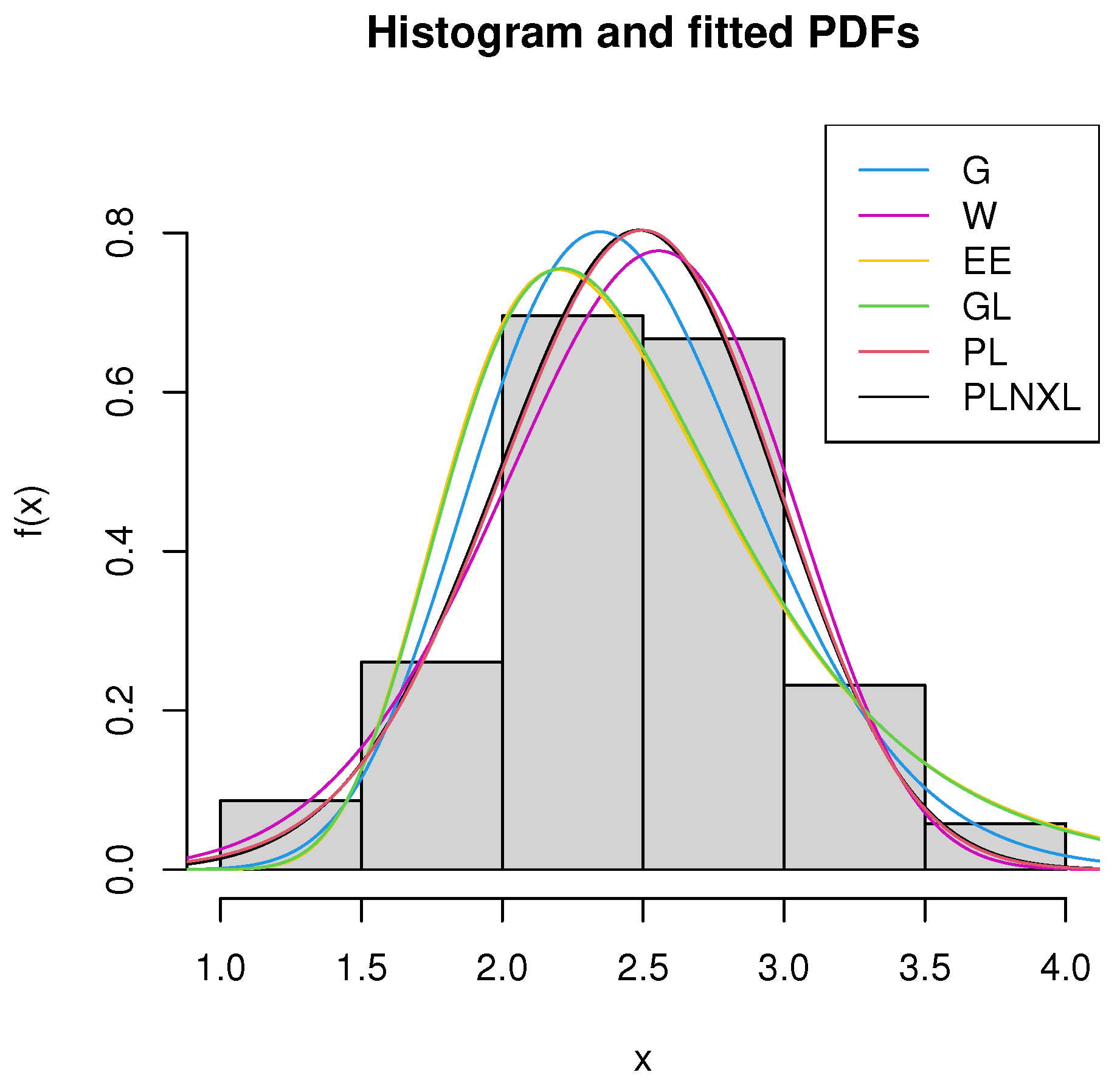
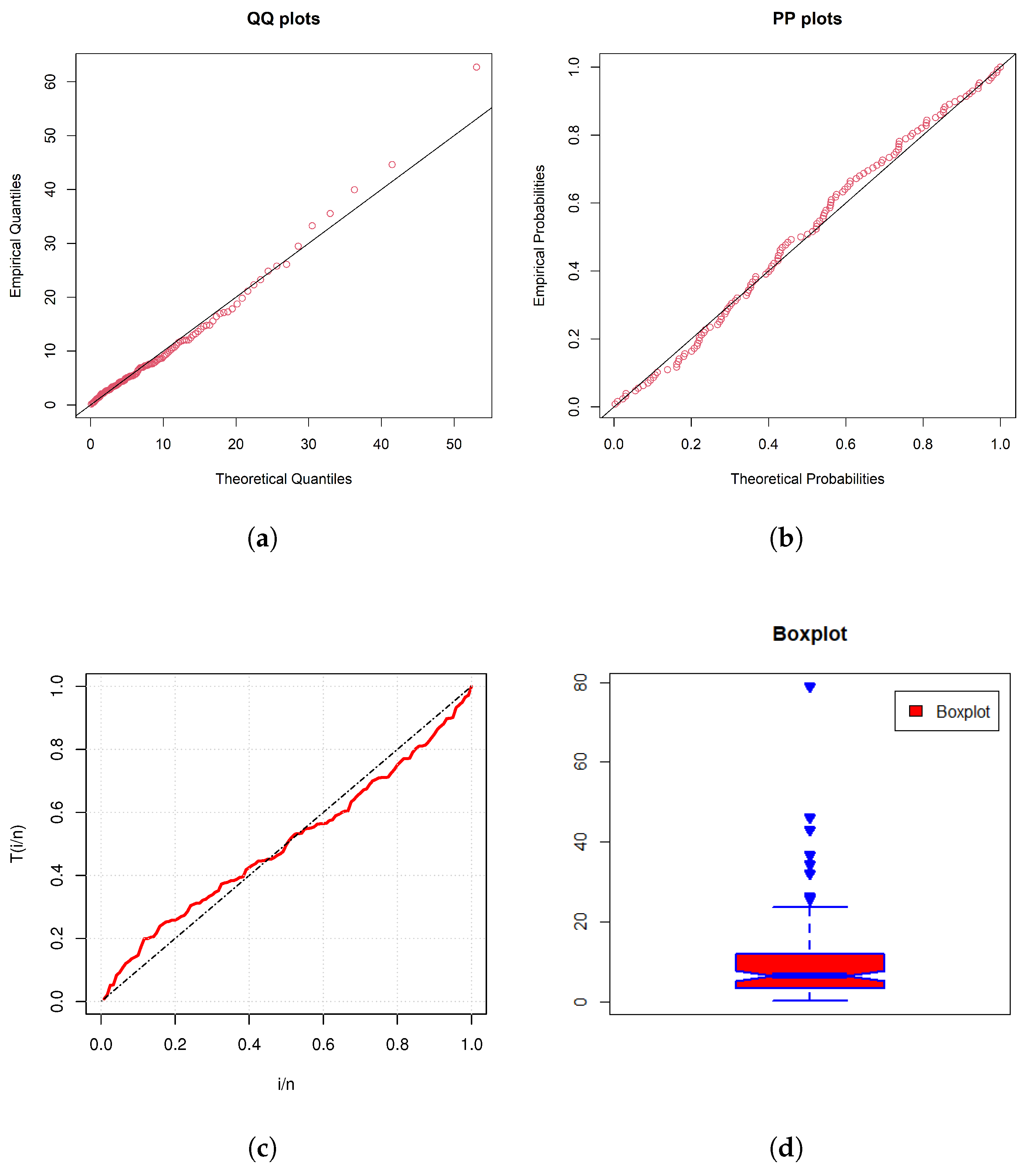
5. Applications to Real-Life Data Sets

The PLNXL distribution is applied in this section for fitting two real data sets. Two actual data sets were taken into consideration. The first set of data given by 1.312, 1.314, 1.479, 1.552, 1.7, 1.803, 1.861, 1.865, 2.14, 2.179, 1.944, 1.958, 1.966, 1.997, 2.006, 2.021, 2.027, 2.055, 2.063, 2.098, 2.24, 2.253, 2.27, 2.272, 2.274, 2.301, 2.301, 2.359, 2.382, 2.382, 2.478, 2.49, 2.511, 2.514, 2.535, 2.554, 2.566, 2.57, 2.586, 2.629, 2.684, 2.697, 2.726, 2.77, 2.773, 2.8, 2.809, 2.818, 2.821, 2.848, 3.067, 3.084, 3.09, 3.096, 3.128, 3.233, 3.433, 3.585, 3.585, 2.224, 2.633, 2.642, 2.648, 2.426, 2.434, 2.435, 2.88, 2.954, 3.012 relates to the failure stresses of 20 mm carbon fibers as reported by [41]. This dataset is also used by [42] as an application for power Lindley distribution. It contains 69 observations. The popularity of these data is driven by the fact that carbon fiber is essential for evaluating a material’s strength and stiffness. Specifically, achieving carbon fiber materials with high stiffness and strength is possible through specialized heat treatment processes, which are highly expensive and costly. Therefore, the development of new distributions that accommodate these characteristics is of utmost importance. The mean and standard deviation of the data are 2.45 and 0.49, respectively. These data exhibit a slight negative skewness, with a skewness value of -0.02, suggesting that the distribution is nearly symmetric, though with a slight leftward tail.

The form of hazard rate function of a dataset is ascertained using a graphical method based on total time on test (TTT) [43]. For the given number of observations n, plotting $T(i/n)$ against $i/n$ yields the empirical TTT plot, where $T(i/n)$ is

$$T(i/n)={\displaystyle \frac{{\sum }_{j=1}^i{X}_{\left(j\right)}+(n-i)X_{\left(i\right)}}{{\sum }_{j=1}^n{X}_{\left(j\right)}}},$$

with $X_{\left(i\right)}$ as the i-th sample order statistic.

Figure 4 includes the quantile–quantile plot (Q-Q), probability–probability plot (P-P), box plot, and the TTT plot corresponding to the first data set.

As can be seen from Figure 4, the data representing the failure stresses of carbon fiber of length 20mm indicate an increasing HRF. Therefore, the PLNXL distribution is fitted to this data set and compared to other established probability distributions that can explain data with an increasing hazard rate. The analysis took into account the following probability distributions:

• Gamma distribution $G\left(\alpha ,\beta \right)$:

  $$f_G\left(x\right)={\displaystyle \frac{{\beta }^{\alpha }}{\mathrm{\Gamma }\left(\alpha \right)}}{x}^{\alpha -1}{e}^{-\beta x},x>0,\alpha >0,\beta >0.$$
• Weibull distribution $W\left(\alpha ,\beta \right)$:

  $$f_W\left(x\right)=\alpha \beta x^{\alpha -1}{e}^{-\beta x^{\alpha }},x>0,\alpha >0,\beta >0.$$
• Exponentiated exponential distribution $EE\left(\alpha ,\beta \right)$ due to [44]:

  $$f_{EE}\left(x\right)=\alpha \beta {(1-e^{-\beta x})}^{\alpha -1}{e}^{-\beta x},x>0,\alpha >0,\beta >0.$$
• Generalized Lindley distribution $GL\left(\alpha ,\beta \right)$ [45]:

  $$f_{GL}\left(x\right)={\displaystyle \frac{\alpha {\beta }^2}{\beta +1}}\left(1+x\right){\left(1-{\displaystyle \frac{1+\beta +\beta x}{1+\beta }}{e}^{-\beta x}\right)}^{\alpha -1}{e}^{-\beta x},x>0,\alpha >0,\beta >0.$$
• Power Lindley distribution $PL\left(\alpha ,\beta \right)$ [42]:

  $$f_{PL}\left(x\right)={\displaystyle \frac{\alpha {\beta }^2}{\beta +1}}\left(1+x^{\alpha }\right)x^{\alpha -1}{e}^{-\beta x^{\alpha }},x>0,\alpha >0,\beta >0.$$

Table 2. Summary of model estimation and related criteria for the first data set.

MODEL	MLEs	K-S	AD	CvM	AIC	BIC
G	$\widehat{\alpha }=23.3819$ (3.9530)	$0.0582$$\left(0.9732\right)$	$0.3339$$\left(0.9104\right)$	$0.0449$$\left(0.9077\right)$	$104.0747$	$108.5429$
	$\widehat{\beta }=9.5385$ (1.6299)
W	$\widehat{\alpha }=5.5021$ (0.3294)	$0.0556$$\left(0.9832\right)$	$0.2723$$\left(0.9573\right)$	$0.0338$$\left(0.9632\right)$	$103.1924$	$107.6607$
	$\widehat{\beta }=0.0047$ (0.0019)
EE	$\widehat{\alpha }=88.2219$ (32.9253)	$0.0949$$\left(0.5625\right)$	$1.1201$$\left(0.2998\right)$	$0.1598$$\left(0.3615\right)$	$113.2403$	$117.7085$
	$\widehat{\beta }=2.0374$ (0.1798)
GL	$\widehat{\alpha }=64.0540$ (23.8138)	$0.0916$$\left(0.6087\right)$	$1.0350$$\left(0.3392\right)$	$0.1467$$\left(0.4006\right)$	$112.2801$	$116.7483$
	$\widehat{\beta }=2.3117$ (0.1850)
PL	$\widehat{\alpha }=3.8679$ (0.3138)	$0.0441$$\left(0.9993\right)$	$0.1592$$\left(0.9978\right)$	$0.0178$$\left(0.9987\right)$	$102.1191$	$106.5873$
	$\widehat{\beta }=0.0496$ (0.0160)
PLNXL	$\widehat{\alpha }=3.3688$ (0.3050)	$0.0423$$\left(0.9997\right)$	$0.1496$$\left(0.9986\right)$	$0.0164$$\left(0.9993\right)$	$101.8314$	$106.2996$
	$\widehat{\beta }=0.1120$ (0.0356)

provides MLEs along with standard errors (in brackets), values for the Kolmogorov–Smirnov (KS) statistic, Anderson–Darling (AD), and Cramer–von Mises (CvM), along with p-values (in brackets) and AIC and BIC values for Data Set 1. The KS, AD, and CvM tests determine whether the observed data follow a specified theoretical distribution. The null hypothesis in each test states that the sample data follow the given distribution. If the p-value of the respective test is below 0.05, the null hypothesis is rejected. As shown in Table 2, PLNXL achieves the lowest AIC and BIC values, outperforming competitive models. Since lower AIC/BIC values indicate better model selection while penalizing unnecessary complexity, these results confirm that PLNXL provides a superior fit to the data. Furthermore, the goodness-of-fit metrics (KS, AD, and CvM) for PLNXL are lower than those for the competitive models, with higher corresponding p-values, further supporting the robustness of PLNXL in capturing the underlying failure time distribution. The fitted PDFs of the models and the histogram of the data are shown in Figure 5. It is evident from Table 2 and Figure 5 that the suggested distribution outperforms the other competing models.

The second data set is given by 0.08, 2.09, 3.48, 4.87, 6.94, 8.66, 13.11, 23.63, 5.09, 7.26, 9.47, 14.24, 25.82, 0.51, 2.54, 3.70, 0.81, 2.62, 3.82, 5.32, 7.32, 10.06, 14.77, 32.15, 14.83, 34.26, 0.90, 2.69, 4.18, 5.34, 7.59, 10.66, 5.41, 7.62, 10.75, 16.62, 43.01, 1.19, 2.75, 4.26, 2.83, 4.33, 5.49, 7.66, 11.25, 17.14, 79.05, 1.35, 1.40, 3.02, 4.34, 5.71, 7.93, 11.79, 18.10, 1.46, 1.76, 3.25, 4.50, 6.25, 8.37, 12.02, 2.02, 3.31, 20.28, 2.02, 3.36, 6.76, 12.07, 21.73, 2.07, 3.36, 0.20, 2.23, 3.52, 4.98, 2.87, 5.62, 7.87, 11.64, 13.80, 25.74, 0.50, 2.46, 4.40, 5.85, 8.26, 11.98, 5.17, 7.28, 9.74, 14.76, 4.51, 6.54, 8.53, 12.03, 2.64, 3.88, 5.32, 7.39, 6.93, 8.65, 12.63, 22.69, 15.96, 36.66, 1.05, 2.69, 6.97, 3.64, 26.31, 10.34, 5.41, 7.63, 17.12, 46.12, 4.23, 1.26, 17.36, 19.13 and records the remission times (in months) of a random sample of 128 bladder cancer patients [46]. The mean and standard deviation of the data are 9.36 and 10.50, respectively. Additionally, the skewness is 3.24, indicating that the distribution is not symmetric but instead exhibits a long right tail. The Q-Q, P-P, TTT, and box plots of the data are represented in Figure 6.

The hazard rate function for the data set of the remission times of a random sample of 128 bladder cancer patients is IBT-shaped, as can be inferred from Figure 6. As a result, the PLNXL distribution is fitted to this data set and examined with a few popular probability distributions that may describe hazard rate data with IBT shapes. The analysis took into account the following probability distributions:

• The generalized inverted exponential distribution $GIE(\alpha ,\beta )$ [47]:

  $$f_{GIE}\left(x\right)=\left({\displaystyle \frac{\alpha \beta }{x^2}}\right)e^{\left({\displaystyle \frac{-\beta }{x}}\right)}{\left(1-e^{\left({\displaystyle \frac{-\beta }{x}}\right)}\right)}^{\alpha -1},x>0,\alpha >0,\beta >0.$$
• The inverse gamma distribution $IG(\alpha ,\beta )$:

  $$f_{IG}\left(x\right)={\displaystyle \frac{{\beta }^{\alpha }}{\mathrm{\Gamma }\left(\alpha \right)}}{\left({\displaystyle \frac{1}{x}}\right)}^{\alpha +1}{e}^{\left({\displaystyle \frac{-\beta }{x}}\right)},x>0,\alpha >0,\beta >0.$$
• The inverse Weibull distribution $IW(\alpha ,\beta )$:

  $$f_{IW}\left(x\right)=\alpha \beta x^{-\left(\beta +1\right)}{e}^{\left(-\alpha x^{-\beta }\right)},x>0,\alpha >0,\beta >0.$$
• The inverse PL distribution $IPL(\alpha ,\beta )$ [48]:

  $$f_{IPL}\left(x\right)={\displaystyle \frac{\alpha {\beta }^2}{1+\beta }}\left({\displaystyle \frac{1+x^{\alpha }}{x^{2\alpha +1}}}\right)e^{\left({\displaystyle \frac{-\beta }{x^{\alpha }}}\right)},x>0,\alpha >0,\beta >0.$$
• The lognormal distribution $LN(\alpha ,\beta )$:

  $$f_{LN}\left(x\right)={\displaystyle \frac{1}{x\beta \sqrt{2\pi }}}{e}^{{\displaystyle \frac{-{\left(log\left(x\right)-\alpha \right)}^2}{2{\beta }^2}}},x>0,\alpha >0,\beta >0.$$
• The Lindley exponential distribution $LE(\alpha ,\beta )$ [49]:

  $$f_{LE}\left(x\right)={\displaystyle \frac{{\alpha }^2\beta e^{-\beta x}{\left(1-e^{-\beta x}\right)}^{\alpha -1}\left(1-log\left(1-e^{-\beta x}\right)\right)}{1+\alpha }},x>0,\alpha >0,\beta >0.$$

For the second data,

Table 3. Summary of model estimation and related criteria for the second data set.

MODEL	MLEs	K-S	AD	CvM	AIC	BIC
GIE	$\widehat{\alpha }=0.7462$ (0.0883)	0.20669 (0.0001)	9.3928 (0.0001)	1.8347 (0.0001)	918.4048	924.1088
	$\widehat{\beta }=1.9945$ (0.2704)
IG	$\widehat{\alpha }=0.7146$ (0.0514)	0.1909 (0.0002)	8.3938 (0.0001)	1.5675 (0.0001)	913.8611	919.5652
	$\widehat{\beta }=1.7756$ (0.2196)
IW	$\widehat{\alpha }=2.4311$ (0.2192)	0.1408 (0.0124)	6.1183 (0.0009)	0.9787 (0.0027)	892.0015	897.7056
	$\widehat{\beta }=0.7521$ (0.0424)
IPL	$\widehat{\alpha }=0.7177$ (0.0412)	0.1481 (0.0073)	6.3977 (0.0006)	1.0213 (0.0021)	895.6256	901.3297
	$\widehat{\beta }=2.9916$ (0.2272)
LN	$\widehat{\alpha }=1.7534$ (0.0948)	0.0617 (0.714)	0.8030 (0.4786)	0.1186 (0.5019)	834.1887	839.8928
	$\widehat{\beta }=1.0731$ (0.0670)
LE	$\widehat{\alpha }=1.5688$ (0.0137)	0.0621 (0.7067)	0.5244 (0.7217)	0.0897 (0.6384)	828.0985	833.8026
	$\widehat{\beta }=0.1094$ (0.1637)
PLNXL	$\widehat{\alpha }=0.6549$ (0.0426)	0.0532 (0.8604)	0.4334 (0.8148)	0.0696 (0.7548)	826.6529	832.3570
	$\widehat{\beta }=0.6819$ (0.0808)

gives MLEs along with standard errors (in brackets) and the values of the KS, AD, and CvM statistics, in addition to the p values (in brackets). Table 3 shows that compared to the IG, IW, GIE, IPL, LN, and LE distributions, the PLNXL distribution has lower values for the KS statistic, AD statistic, Cramer–von Mises statistic, AIC, and BIC. Figure 7 represents the plot of fitted PDFs of the models and the empirical histogram. It is evident that the PLNXL distribution fits the empirical histogram better than the fits of the other classical distributions investigated here. In summary, the PLNXL distribution for modeling lifetime data sets may provide a strong alternative to the earlier models.

6. Conclusions

This article introduces a new lifetime distribution, namely, the power length-biased new XLindley distribution. Among its many useful characteristics are closed-form expressions for the survival function, failure rate function, cumulative distribution function, and raw moments. Specifically, the proposed distribution can accommodate datasets with increasing, decreasing, and IBT-shaped hazard rate functions. Furthermore, the mean residual life function of the distribution exhibits decreasing, increasing, and bathtub-shaped patterns. An algorithm for generating random observations from this distribution is also provided. Model parameters are estimated using the maximum likelihood estimation method. To evaluate the performance of the maximum likelihood estimators, a comprehensive simulation study is conducted. Finally, the applicability of the proposed model is demonstrated using two real datasets. The results show that our model outperforms several popular existing models, suggesting that it may be effective in a wide range of practical scenarios beyond the scope of this study.

The proposed model has certain limitations. While parameter estimation is generally straightforward, numerical optimization techniques are required, potentially increasing computational complexity. Furthermore, in small sample scenarios or highly skewed data, parameter identifiability issues may arise, necessitating the use of robust estimation techniques such as penalized likelihood methods. Future research directions include extending PLNXL to a Bayesian framework, allowing for prior information incorporation and uncertainty quantification, as well as adapting it for censored data scenarios common in reliability and survival analysis. Additionally, investigating PLNXL in multivariate survival settings or as a baseline hazard function in frailty models could further enhance its applicability. Despite these challenges, the PLNXL model offers a promising alternative to the existing lifetime distributions, expanding the toolkit available for modeling real-world failure time data in engineering, medical, and reliability applications. As future work, the reliability of the distribution may be estimated using deep learning methods [50], and the distribution can be modified to suggest new models. Additionally, the distribution parameters can be estimated using the ranked set sampling method [51,52,53].

References

1. Bennett, S. Log-logistic regression models for survival data. Appl. Stat. 1983, 32, 165–171. [Google Scholar] [CrossRef]
2. Efron, B. Logistic regression, survival analysis, and the Kaplan-Meier curve. J. Am. Stat. Assoc. 1988, 83, 414–425. [Google Scholar] [CrossRef]
3. Langlands, A.; Pocock, S.; Kerr, G.; Gore, S. Long-term survival of patients with breast cancer: A study of the curability of the disease. Br. Med. J. 1979, 2, 1247–1251. [Google Scholar] [CrossRef]
4. Aalen, O.O.; Gjessing, H.K. Understanding the shape of the hazard rate: A process point of view. Stat. Sci. 2001, 16, 1–22. [Google Scholar] [CrossRef]
5. Bae, S.J.; Kuo, W.; Kvam, P.H. Degradation models and implied lifetime distributions. Reliab. Eng. Syst. Saf. 2007, 92, 601–608. [Google Scholar] [CrossRef]
6. Crowder, M.J.; Kimber, A.C.; Smith, R.L.; Sweeting, T.J. Statistical Analysis of Reliability Data; Chapman and Hall/CRC: Boca Raton, FL, USA, 1991. [Google Scholar]
7. Lai, C.; Xie, M. Stochastic Aging and Dependence for Reliability; Springer: New York, NY, USA, 2006. [Google Scholar]
8. Lindley, D. Fiducial distributions and Bayes’ theorem. J. R. Stat. Soc. Ser. B 1958, 20, 102–107. [Google Scholar] [CrossRef]
9. Benchiha, S.A.; Al-Omari, A.I. Generalized quasi Lindley distribution: Theoretical properties, estimation methods and applications. Electron. J. Appl. Stat. Anal. 2021, 14, 167. [Google Scholar]
10. Irshad, M.; Maya, R.; Al-Omari, A.I.; Arun, S.; Alomani, G. The extended Farlie-Gumbel-Morgenstern bivariate Lindley distribution: Concomitants of order statistics and estimation. Electron. J. Appl. Stat. Anal. 2021, 14, 373–388. [Google Scholar]
11. Benchiha, S.; Al-Omari, A.I.; Alotaibi, N.; Shrahili, M. Weighted generalized quasi Lindley distribution: Different methods of estimation, applications for COVID-19 and engineering data. AIMS Math. 2021, 6, 11850–11878. [Google Scholar] [CrossRef]
12. Chouia, S.; Zeghdoudi, H. The XLindley distribution: Properties and application. J. Stat. Theory Appl. 2021, 20, 318–327. [Google Scholar] [CrossRef]
13. Khodja, N.; Gemeay, A.M.; Zeghdoudi, H.; Karakaya, K.; Alshangiti, A.M.; Bakr, M.E.; Balogun, O.S.; Muse, A.H.; Hussam, E. Modeling voltage real data set by a new version of Lindley distribution. IEEE Access 2023, 11, 67220–67229. [Google Scholar] [CrossRef]
14. Metiri, F.; Zeghdoudi, H.; Ezzebsa, A. On the characterisation of XLindley distribution by truncated moments. properties and application. Oper. Res. Decis. 2022, 32, 97–109. [Google Scholar]
15. Zinhom, E.; Nassar, M.; Radwan, S.; Elmasry, A. The wrapped XLindley distribution. Environ. Ecol. Stat. 2003, 30, 669–686. [Google Scholar] [CrossRef]
16. Etaga, H.O.; Nwankwo, M.P.; Oramulu, D.O.; Anabike, I.C.; Obulezi, O.J. The double XLindley distribution: Properties and applications. Sch. J. Phys. Math. Stat. 2023, 10, 192–202. [Google Scholar] [CrossRef]
17. Beghriche, A.; Tashkandy, Y.A.; Bakr, M.E.; Zeghdoudi, H.; Gemeay, A.M.; Hossain, M.M.; Muse, A.H. The inverse XLindley distribution: Properties and application. IEEE Access 2023, 11, 47272–47281. [Google Scholar] [CrossRef]
18. MirMostafaee, S. The exponentiated new XLindley distribution: Properties, and Applications. J. Data Sci. Model. 2023, 2, 185–208. [Google Scholar]
19. Gemeay, A.M.; Ezzebsa, A.; Zeghdoudi, H.; Tanış, C.; Tashkandy, Y.A.; Bakr, M.; Kumar, A. The power new XLindley distribution: Statistical inference, fuzzy reliability, and applications. Heliyon 2024, 10, e36594. [Google Scholar] [CrossRef]
20. Alghamdi, F.M.; Ahsan-ul Haq, M.; Hussain, M.N.S.; Hussam, E.; Almetwally, E.M.; Aljohani, H.M.; Mustafa, M.S.; Alshawarbeh, E.; Yusuf, M. Discrete poisson quasi-XLindley distribution with mathematical properties, regression model, and data analysis. J. Radiat. Res. Appl. Sci. 2024, 17, 100874. [Google Scholar] [CrossRef]
21. Alomair, A.M.; Ahmed, M.; Tariq, S.; Ahsan-ul Haq, M.; Talib, J. An exponentiated XLindley distribution with properties, inference and applications. Heliyon 2024, 10, e25472. [Google Scholar] [CrossRef]
22. Musekwa, R.R.; Makubate, B. A flexible generalized XLindley distribution with application to engineering. Sci. Afr. 2024, 24, e02192. [Google Scholar] [CrossRef]
23. Alsadat, N. A new extension of XLindley distribution with mathematical properties, estimation, and application on the rainfall data. Heliyon 2024, 10, e38143. [Google Scholar] [CrossRef] [PubMed]
24. Kouadria, M.; Zeghdoudi, H. The truncated new-XLindley distribution with applications. J. Comput. Anal. Appl. 2025, 34, 53–64. [Google Scholar]
25. Rao, C.R. On discrete distributions arising out of methods of ascertainment. Sankhya A 1965, 27, 311–324. [Google Scholar]
26. ul Haq, M.A.; Usman, R.M.; Hashmi, S.; Al-Omeri, A.I. The Marshall-Olkin length-biased exponential distribution and its applications. J. King Saud Univ.-Sci. 2019, 31, 246–251. [Google Scholar] [CrossRef]
27. Rajagopalan, V.; Ganaie, R.A.; Rather, A.A. A new length biased distribution with applications. Sci. Technol. Dev. 2019, 8, 161–174. [Google Scholar]
28. Hassan, A.S.; Almetwally, E.M.; Khaleel, M.A.; Nagy, H.F. Weighted power Lomax distribution and its length biased version: Properties and estimation based on censored samples. Pak. J. Stat. Oper. Res. 2021, 17, 343–356. [Google Scholar] [CrossRef]
29. Chaito, T.; Khamkong, M. The length–biased Weibull–Rayleigh distribution for application to hydrological data. Lobachevskii J. Math. 2021, 42, 3253–3265. [Google Scholar] [CrossRef]
30. Alzoubi, L. Length-biased Loai distribution: Statistical properties and application. Electron. J. Appl. Stat. Anal. 2024, 17, 278. [Google Scholar]
31. Bryson, M.; Siddique, M. Some criteria for aging. J. Am. Stat. Assoc. 1969, 64, 1472–1483. [Google Scholar] [CrossRef]
32. Gupta, R.; Akman, O. Mean residual life function for certain types of non-monotonic ageing. Commun. Stat.-Stoch. Model. 1995, 11, 219–225. [Google Scholar]
33. Rényi, A. On measures of information and entropy. In Proceedings of the Fourth Berkeley Symposium on Mathematics, Statistics and Probability 1960; University of California Press: Berkeley, CA, USA, 1961; pp. 547–561. [Google Scholar]
34. Tsallis, C. Possible generalization of Boltzmann-Gibbs statistics. J. Stat. Phys. 1988, 52, 479–487. [Google Scholar] [CrossRef]
35. Kızılaslan, F. Classical and bayesian estimation of reliability in a multicomponent stress–strength model based on the proportional reversed hazard rate mode. Math. Comput. Simul. 2017, 136, 36–62. [Google Scholar] [CrossRef]
36. Agiwal, V. Bayesian estimation of stress strength reliability from inverse Chen distribution with application on failure time data. Ann. Data Sci. 2023, 10, 317–347. [Google Scholar] [CrossRef]
37. Xu, A.; Fang, G.; Zhuang, L.; Gu, C. A multivariate student-t process model for dependent tail-weighted degradation data. IISE Trans. 2024. [Google Scholar] [CrossRef]
38. Zhuang, L.; Xu, A.; Wang, Y.; Tang, Y. Remaining useful life prediction for two-phase degradation model based on reparameterized inverse Gaussian process. Eur. J. Oper. Res. 2024, 319, 877–890. [Google Scholar] [CrossRef]
39. Gradshteyn, I.; Ryzhik, I. Tables of Integrals, Series, and Products; Academic Press: New York, NY, USA, 2007. [Google Scholar]
40. Lehmann, L.; Casella, G. Theory of Point Estimation; Springer: New York, NY, USA, 1998. [Google Scholar]
41. Bader, M.G.; Priest, A.M. Statistical aspects of fibre and bundle strength in hybrid composites. In Progress in Science and Engineering Composites. Vol. 4th International Conference on Composite Materials (ICCM-IV); Hayashi, T., Kawata, K., Umekawa, S., Eds.; Japan Society Society for Composite Materials: Tokyo, Japan, 1982; pp. 1129–1136. [Google Scholar]
42. Ghitany, M.; Al-Mutairi, D.; Balakrishnan, N.; Al-Enezi, L. Power Lindley distribution and associated inference. Comput. Stat. Data Anal. 2013, 64, 20–33. [Google Scholar] [CrossRef]
43. Aarset, M. How to identify a bathtub hazard rate. IEEE Trans. Reliab. 1987, 36, 106–108. [Google Scholar] [CrossRef]
44. Gupta, R.; Kundu, D. Exponentiated exponential family: An alternative to gamma and Weibull distributions. Biom. J. 2001, 43, 117–130. [Google Scholar] [CrossRef]
45. Nadarajah, S.; Bakouch, H.; Tahmasbi, R. A generalized Lindley distribution. Sankhya B 2011, 73, 331–359. [Google Scholar] [CrossRef]
46. Lee, E.; Wang, J. Statistical Methods for Survival Data Analysis; John Wiley and Sons: New York, NY, USA, 2003. [Google Scholar]
47. Abouammoh, A.; Alshingiti, A. Reliability estimation of generalized inverted exponential distribution. J. Stat. Comput. Simul. 2009, 79, 1301–1315. [Google Scholar] [CrossRef]
48. Barco, K.; Mazucheli, J.; Janeiro, V. The inverse power Lindley distribution. Commun. Stat.-Simul. Comput. 2017, 46, 6308–6323. [Google Scholar] [CrossRef]
49. Bhati, D.; Malik, M.; Vaman, H. Lindley–exponential distribution: Properties and applications. Metron 2015, 73, 335–357. [Google Scholar] [CrossRef]
50. Xu, A.; Wang, R.; Weng, X.; Wu, Q.; Zhuang, L. Strategic integration of adaptive sampling and ensemble techniques in federated learning for aircraft engine remaining useful life prediction. Appl. Soft Comput. 2005, 175, 113067. [Google Scholar] [CrossRef]
51. Al-Omari, A.I. The efficiency of l ranked set sampling in estimating the distribution function. Afr. Mat. 2015, 26, 1457–1466. [Google Scholar] [CrossRef]
52. Al-Omari, A.I.; Bouza, C.N. Review of ranked set sampling: Modifications and applications. Rev. Investig. Oper. 2014, 3, 215–240. [Google Scholar]
53. Al-Omari, A.I. Estimation of the population median of symmetric and asymmetric distributions using double robust extreme ranked set sampling. Investig. Oper. 2010, 31, 199–207. [Google Scholar]
Figure 1. The PDF plots of PLNXL for some combinations of the parameters.
Mathematics 13 01394 g001
Figure 2. The HRF plot of PLNXL for the cases (a) α = 0.4 , β = 0.5 , (b) α = 0.6 , β = 0.8 , and (c) α = 2.05 , β = 0.09 .
Mathematics 13 01394 g002
Figure 3. The MRLF plot of PLNXL for the cases (a) α = 0.6 , β = 0.2 , (b) α = 0.5 , β = 0.5 , and (c) α = 1.5 , β = 0.08 .
Mathematics 13 01394 g003
Figure 4. The (a) Q-Q, (b) P-P, (c) TTT, and (d) box plots for carbon fiber of length 20 mm data.
Mathematics 13 01394 g004
Figure 5. Fitted PDFs and histogram for the first data set.
Mathematics 13 01394 g005
Figure 6. The (a) QQ, (b) PP, (c) TTT, and (d) box plots for the data representing the remission times of a random sample of 128 bladder cancer patients.
Mathematics 13 01394 g006
Figure 7. Fitted PDFs and histogram for the second data set.
Mathematics 13 01394 g007