

Adaptive Terminal Sliding Mode Control for a Quadrotor System with Barrier Function Switching Law

Abstract
1. Introduction
2. System Description
3. Control Design
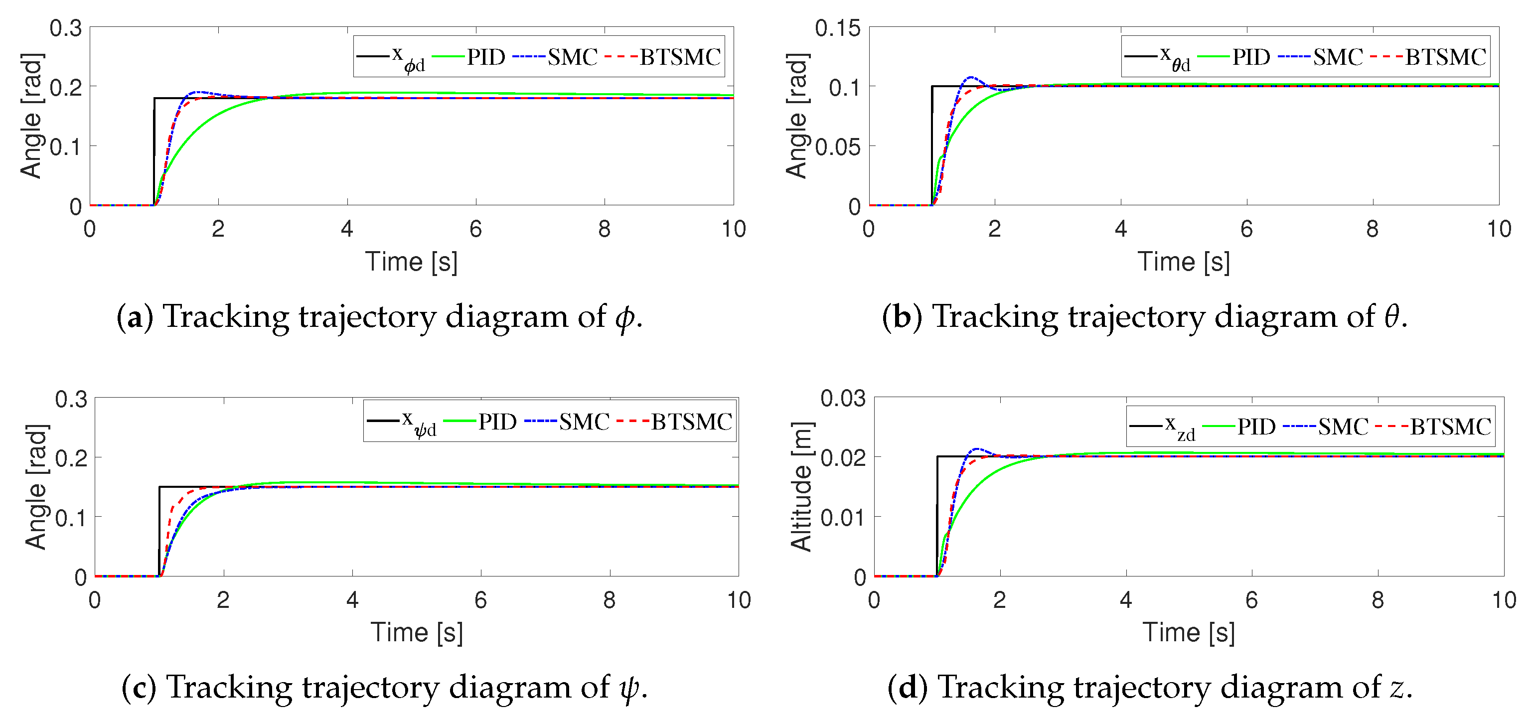
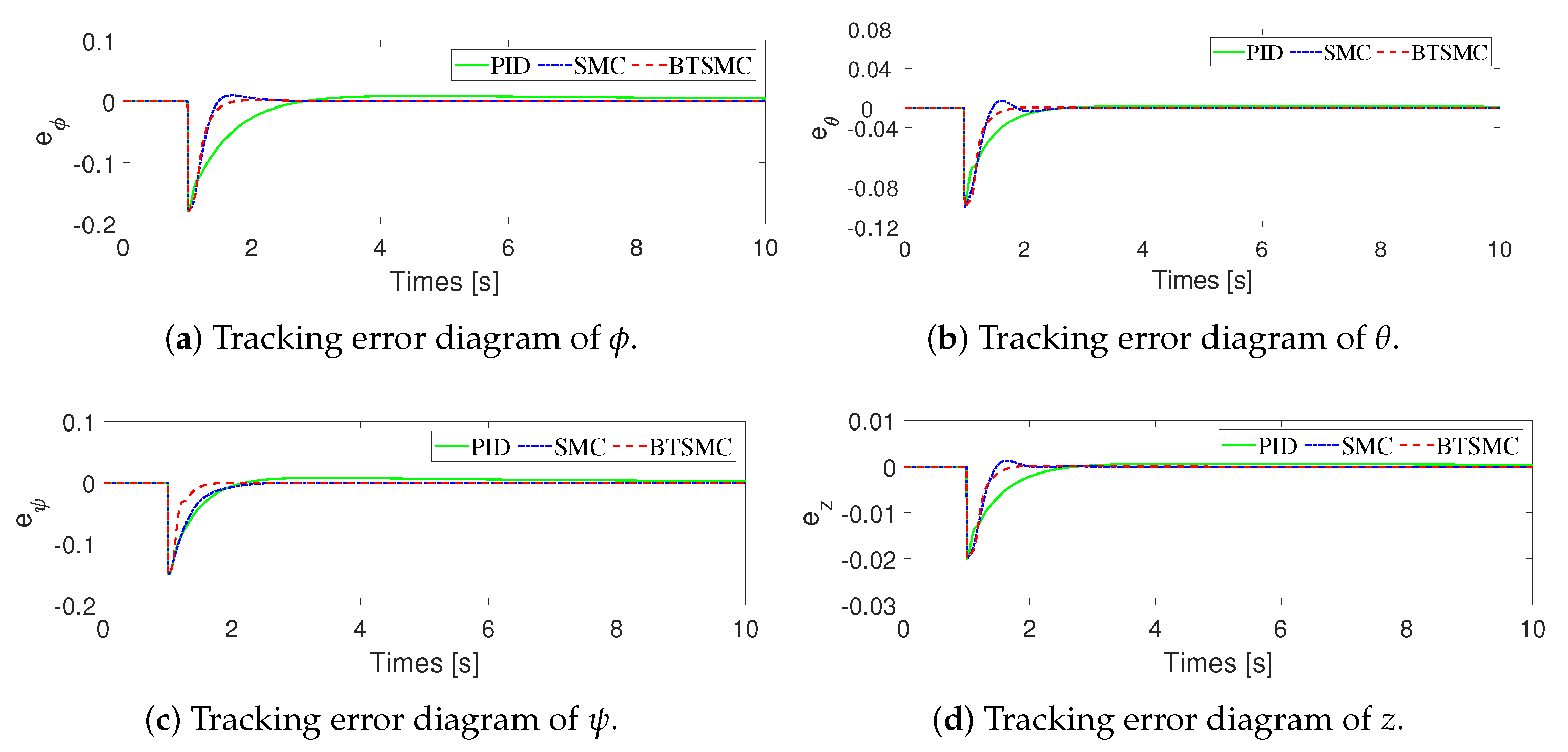
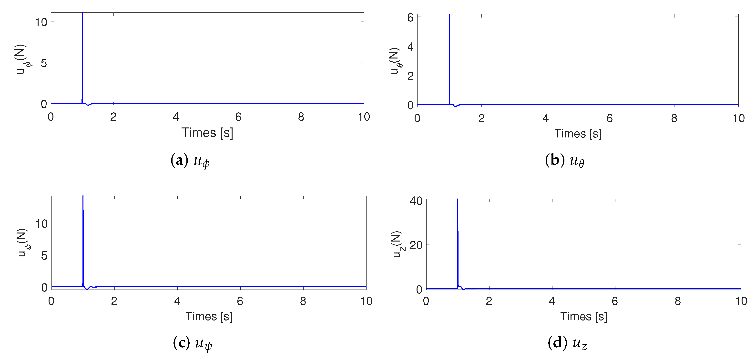
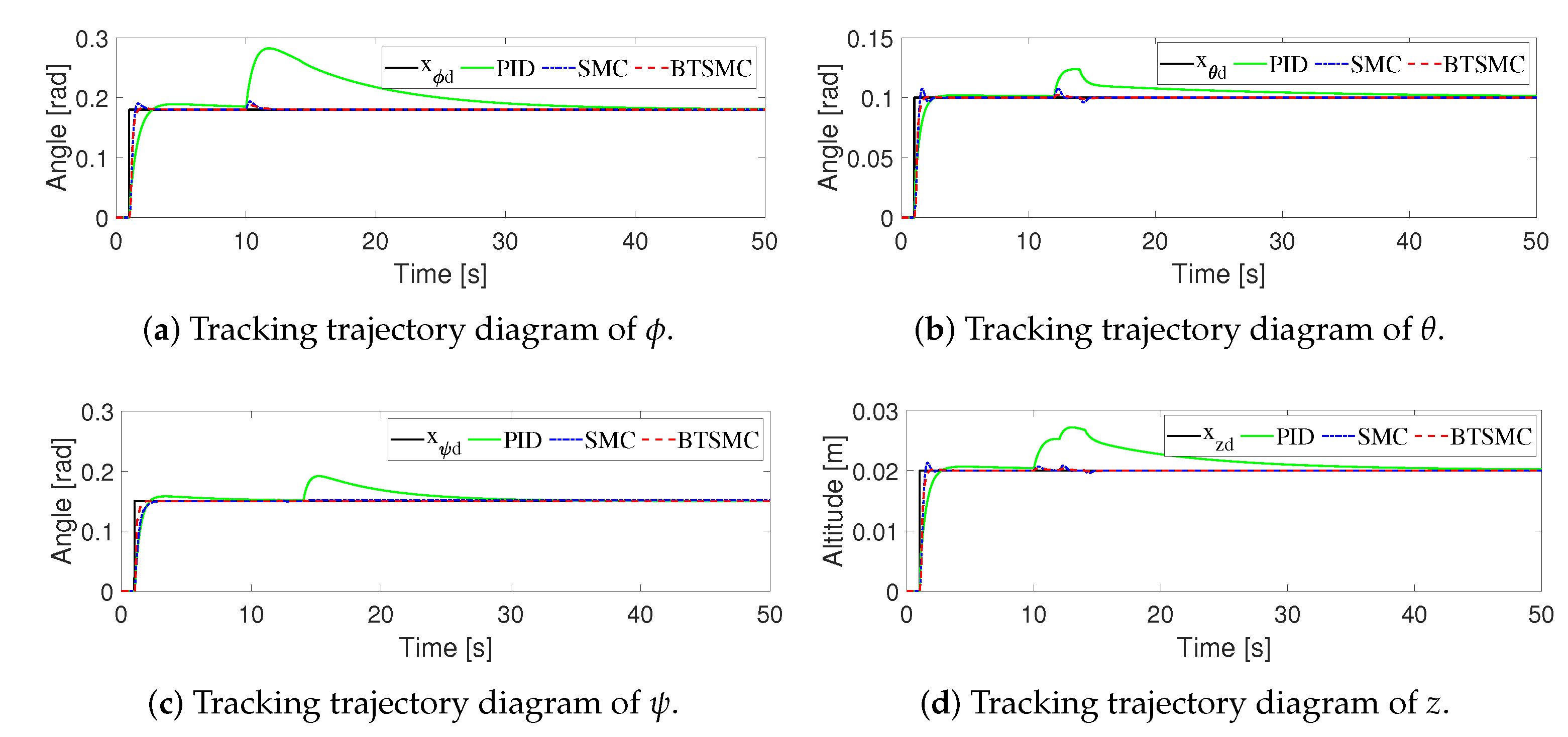
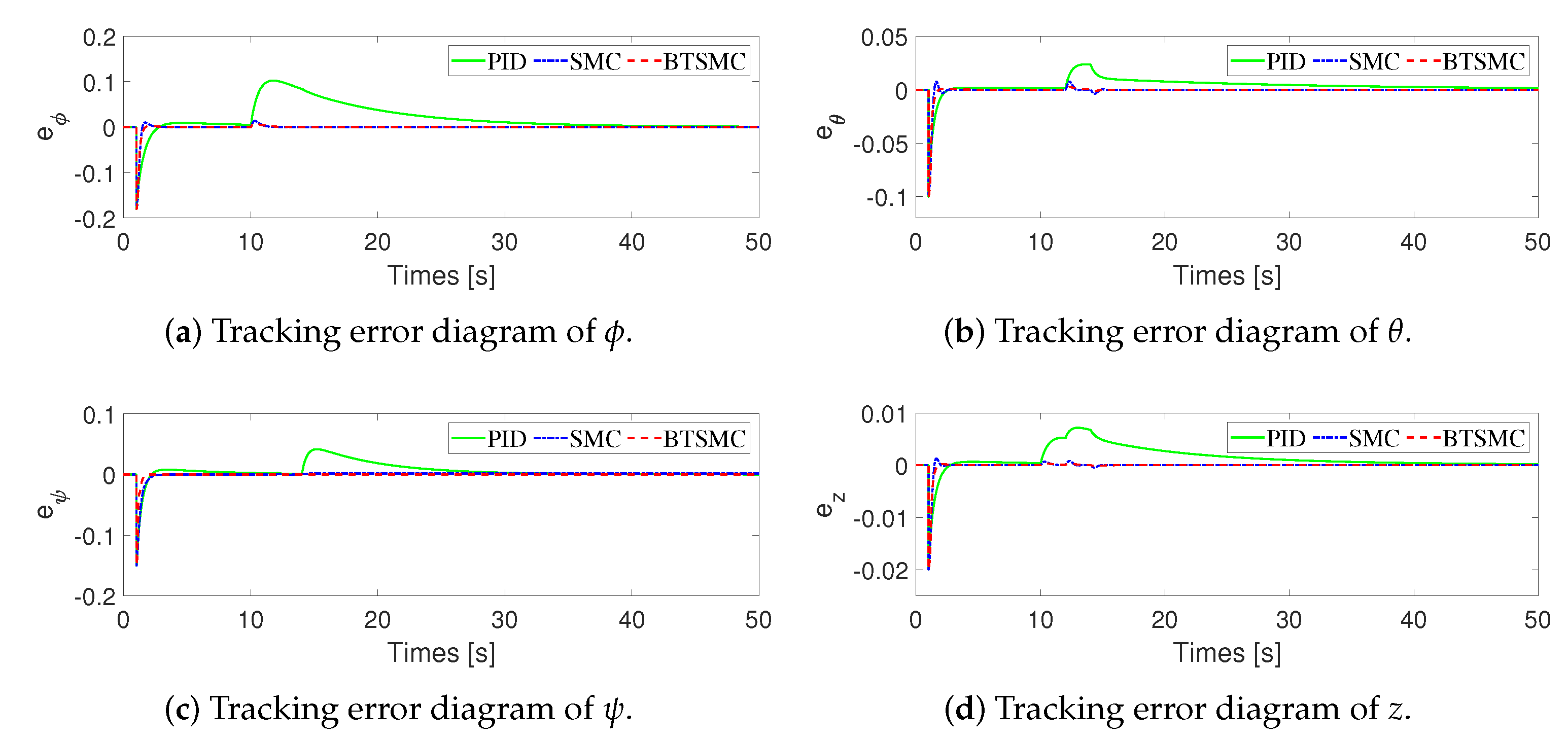
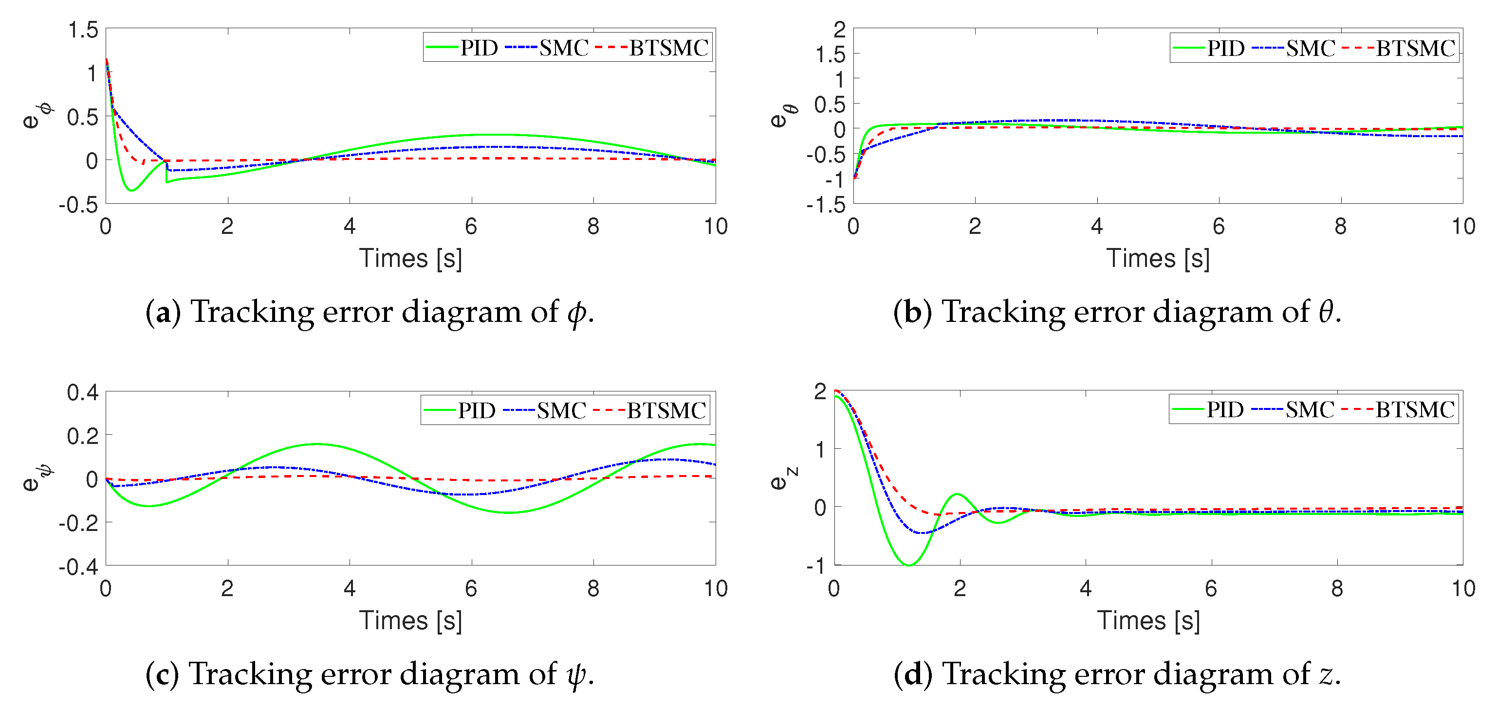
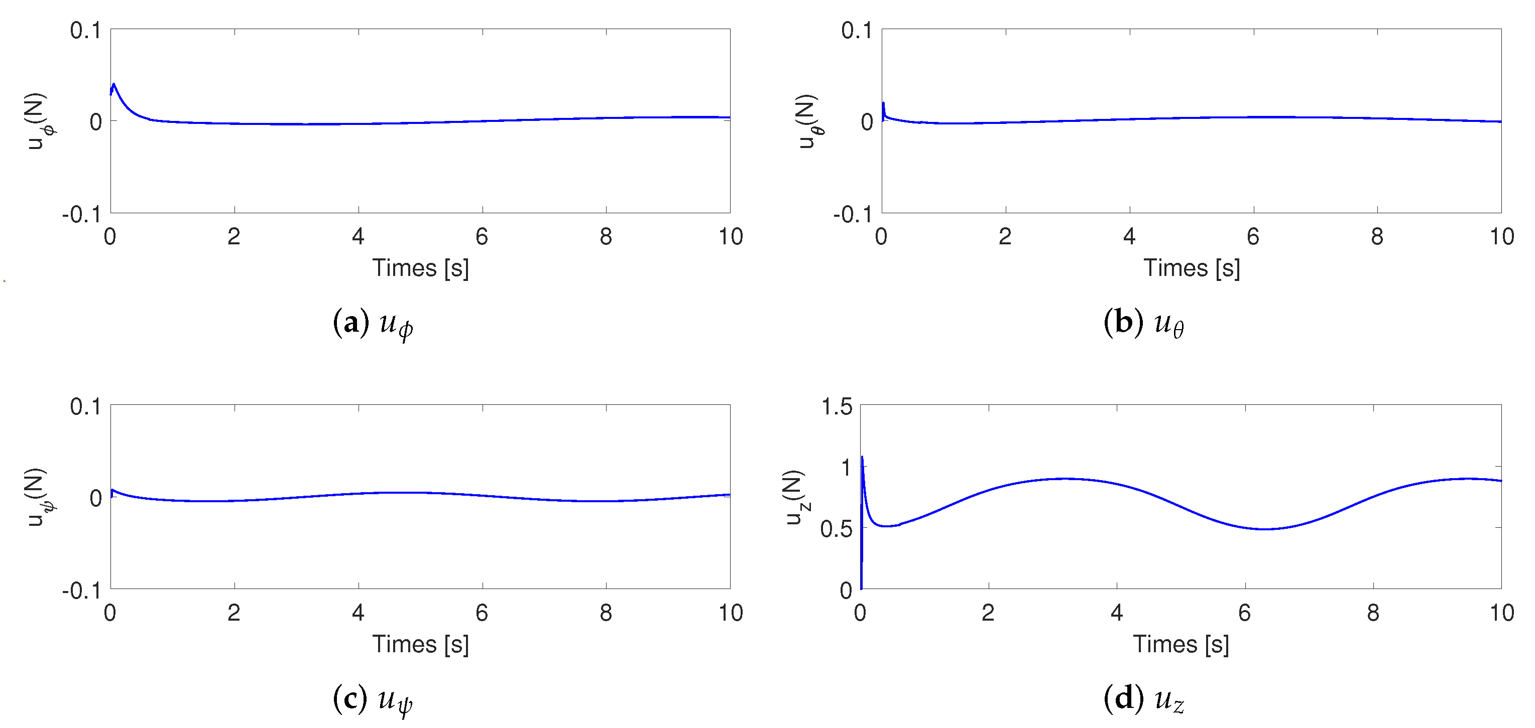
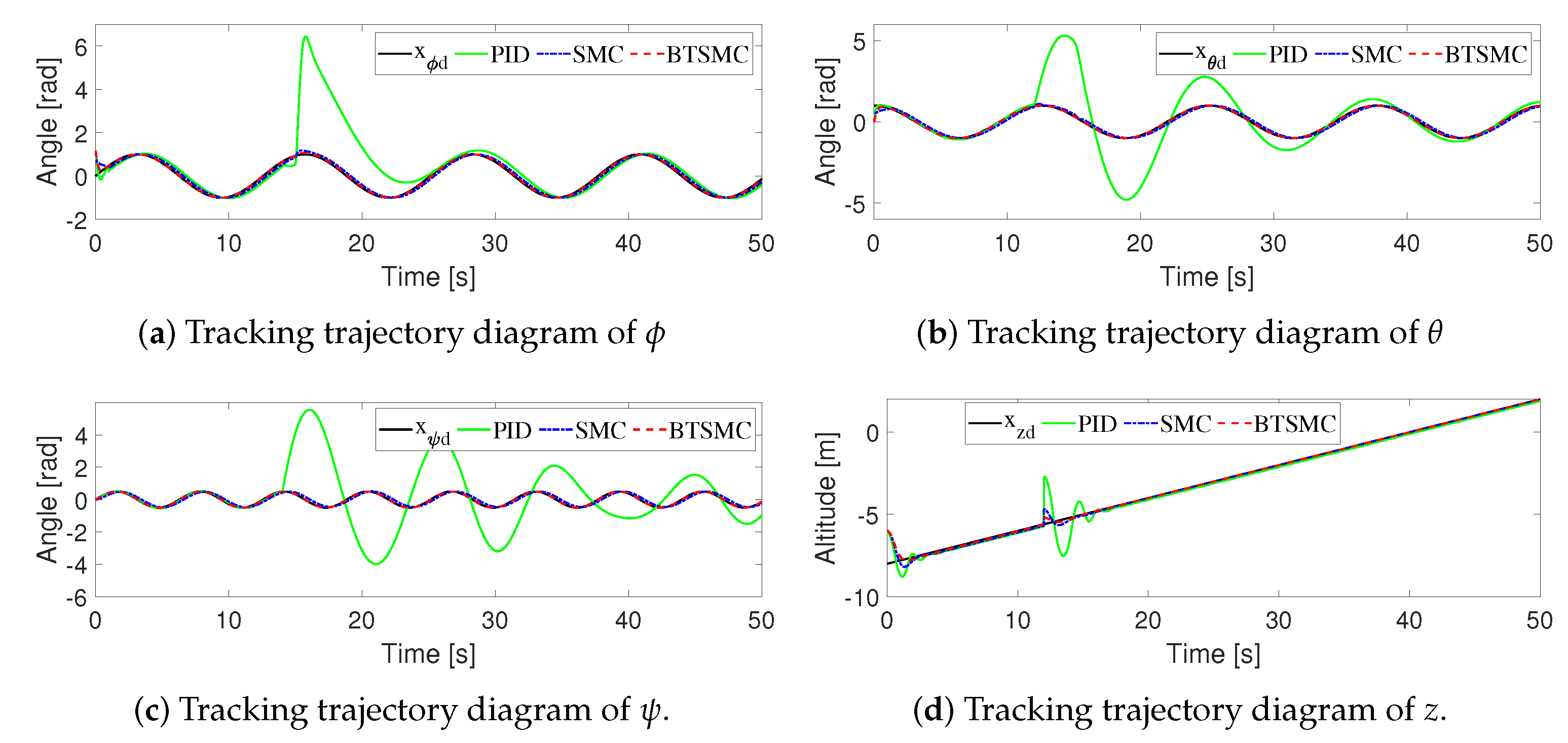
4. Simulations
5. Conclusions
Author Contributions
Funding
Data Availability Statement
Conflicts of Interest
References
- Qi, J.; Guo, J.; Wang, M.; Wu, C.; Ma, Z. Formation tracking and obstacle avoidance for multiple quadrotors with static and dynamic obstacles. IEEE Robot. Autom. Lett. 2022, 7, 1713–1720. [Google Scholar] [CrossRef]
- Elyaalaoui, K.; Labbadi, M.; Boubaker, S.; Kamel, S.; Alsubaei, F.S. On novel fractional-order trajectory tracking control of quadrotors: A predefined-time guarantee performance approach. Mathematics 2023, 11, 3582. [Google Scholar] [CrossRef]
- Li, Z.; Wang, Q.; Zhang, T.; Ju, C.; Suzuki, S.; Namiki, A. UAV high-voltage power transmission line autonomous correction inspection system based on object detection. IEEE Sensors J. 2023, 23, 10215–10230. [Google Scholar] [CrossRef]
- Yan, D.; Zhang, W.; Chen, H.; Shi, J. Robust control strategy for multi-UAVs system using MPC combined with Kalman-consensus filter and disturbance observer. ISA Trans. 2023, 135, 35–51. [Google Scholar] [CrossRef]
- Wen, G.; Hao, W.; Feng, W.; Gao, K. Optimized backstepping tracking control using reinforcement learning for quadrotor unmanned aerial vehicle system. IEEE Trans. Syst. Man Cybern. Syst. 2021, 52, 5004–5015. [Google Scholar] [CrossRef]
- Borbolla-Burillo, P.; Sotelo, D.; Frye, M.; Garza-Castañón, L.E.; Juárez-Moreno, L.; Sotelo, C. Design and Real-Time Implementation of a Cascaded Model Predictive Control Architecture for Unmanned Aerial Vehicles. Mathematics 2024, 12, 739. [Google Scholar] [CrossRef]
- Ulu, B.; Savaş, S.; Ergin, Ö.F.; Ulu, B.; Kırnap, A.; Bingöl, M.S.; Yıldırım, Ş. Tuning the Proportional–Integral–Derivative Control Parameters of Unmanned Aerial Vehicles Using Artificial Neural Networks for Point-to-Point Trajectory Approach. Sensors 2024, 24, 2752. [Google Scholar] [CrossRef]
- Hanif, A.; Putro, I.; Riyadl, A.; Sudiana, O.; Hakiki; Irwanto, H.Y. Towards High-Precision Quadrotor Trajectory Following Capabilities: Modelling, Parameter Estimation, and LQR Control. Latv. J. Phys. Tech. Sci. 2024, 61, 89–104. [Google Scholar] [CrossRef]
- Hou, Z.; Lu, P.; Tu, Z. Nonsingular terminal sliding mode control for a quadrotor UAV with a total rotor failure. Aerosp. Sci. Technol. 2020, 98, 105716. [Google Scholar] [CrossRef]
- Mofid, O.; Mobayen, S. Adaptive sliding mode control for finite-time stability of quad-rotor UAVs with parametric uncertainties. ISA Trans. 2018, 72, 1–14. [Google Scholar] [CrossRef]
- Shao, X.; Sun, G.; Yao, W.; Liu, J.; Wu, L. Adaptive sliding mode control for quadrotor UAVs with input saturation. IEEE/ASME Trans. Mechatronics 2021, 27, 1498–1509. [Google Scholar] [CrossRef]
- Eltayeb, A.; Rahmat, M.F.; Basri, M.A.M. Sliding mode control design for the attitude and altitude of the quadrotor UAV. Int. J. Smart Sens. Intell. Syst. 2020, 13, 1. [Google Scholar] [CrossRef]
- Wang, Q.; Wang, W.; Suzuki, S.; Namiki, A.; Liu, H.; Li, Z. Design and implementation of UAV velocity controller based on reference model sliding mode control. Drones 2023, 7, 130. [Google Scholar] [CrossRef]
- Fu, D.; Zhao, X.; Zhu, J. A novel robust super-twisting nonsingular terminal sliding mode controller for permanent magnet linear synchronous motors. IEEE Trans. Power Electron. 2021, 37, 2936–2945. [Google Scholar] [CrossRef]
- Baek, J.; Kang, M. A synthesized sliding-mode control for attitude trajectory tracking of quadrotor UAV systems. IEEE/ASME Trans. Mechatronics 2023, 28, 2189–2199. [Google Scholar] [CrossRef]
- Villa, D.K.; Brandão, A.S.; Sarcinelli-Filho, M. Adaptive sliding mode control applied to quadrotors—A practical comparative study. J. Frankl. Inst. 2023, 360, 11578–11599. [Google Scholar] [CrossRef]
- Liu, B.; Wang, Y.; Sepestanaki, M.A.; Pouzesh, M.; Mobayen, S.; Rouhani, S.H.; Fekih, A. Event-trigger-based adaptive barrier function higher-order global sliding mode control technique for quadrotor UAVs. IEEE Trans. Aerosp. Electron. Syst. 2024, 60, 5674–5684. [Google Scholar] [CrossRef]
- Liu, Z.G.; Shi, Y.Y.; Sun, W.; Su, S.F. Direct Fuzzy Adaptive Regulation for High-Order Delayed Systems: A Lyapunov–Razumikhin Function Method. IEEE Trans. Cybern. 2024, 54, 1894–1906. [Google Scholar] [CrossRef]
- Madebo, M.M. Neuro-fuzzy based Adaptive Sliding Mode Control of Quadrotor UAV in the Presence of Matched and Unmatched Uncertainties. IEEE Access 2024, 12, 117745–117760. [Google Scholar] [CrossRef]
- Nguyen, N.P.; Oh, H.; Moon, J. Continuous nonsingular terminal sliding-mode control with integral-type sliding surface for disturbed systems: Application to attitude control for quadrotor UAVs under external disturbances. IEEE Trans. Aerosp. Electron. Syst. 2022, 58, 5635–5660. [Google Scholar] [CrossRef]
- Yang, T.; Deng, Y.; Li, H.; Sun, Z.; Cao, H.; Wei, Z. Fast integral terminal sliding mode control with a novel disturbance observer based on iterative learning for speed control of PMSM. ISA Trans. 2023, 134, 460–471. [Google Scholar] [CrossRef] [PubMed]
- Mo, H.; Farid, G. Nonlinear and adaptive intelligent control techniques for quadrotor uav—A survey. Asian J. Control. 2019, 21, 989–1008. [Google Scholar] [CrossRef]
- Chen, Q.; Zhang, J.; Zhang, C.; Zhou, H.; Jiang, X.; Yang, F.; Wang, Y. CFD analysis and RBFNN-based optimization of spraying system for a six-rotor unmanned aerial vehicle (UAV) sprayer. Crop Prot. 2023, 174, 106433. [Google Scholar] [CrossRef]
- Shu, R.; Jia, Q.; Wu, Y.; Liao, H.; Zhang, C. Robust Active Fault-Tolerant Configuration Control for Spacecraft Formation via Learning RBFNN Approaches. J. Aerosp. Eng. 2024, 37, 04024007. [Google Scholar] [CrossRef]
- Xiong, J.J.; Guo, N.H.; Mao, J.; Wang, H.D. Self-tuning sliding mode control for an uncertain coaxial octorotor UAV. IEEE Trans. Syst. Man Cybern. Syst. 2022, 53, 1160–1171. [Google Scholar] [CrossRef]
- Mahmood, A.; ur Rehman, F.; Okasha, M.; Saeed, A. Neural adaptive sliding mode control for camera positioner quadrotor UAV. Int. J. Aeronaut. Space Sci. 2024, 26, 733–747. [Google Scholar] [CrossRef]
- Ranjan, S.; Majhi, S. Adaptive neural predefined-time attitude control of an uncertain quadrotor UAV with actuator fault. IEEE Trans. Circuits Syst. II Express Briefs 2024, 71, 4939–4943. [Google Scholar] [CrossRef]
- Wang, K.; Liu, Y.; Huang, C.; Bao, W. Water surface flight control of a cross domain robot based on an adaptive and robust sliding mode barrier control algorithm. Aerospace 2022, 9, 332. [Google Scholar] [CrossRef]
- Adıgüzel, F.; Kurtuluş, K.; Türker, T. A Gain Scheduling Attitude Controller with NN Supervisor for Quadrotor UAVs. Int. J. Control Autom. Syst. 2024, 22, 3777–3791. [Google Scholar] [CrossRef]
- Husain, S.S.; Al-Dujaili, A.Q.; Jaber, A.A.; Humaidi, A.J.; Al-Azzawi, R.S. Design of a robust controller based on barrier function for vehicle steer-by-wire systems. World Electr. Veh. J. 2024, 15, 17. [Google Scholar] [CrossRef]
- Tian, D.; Song, X. Addressing complex state constraints in the integral barrier Lyapunov function-based adaptive tracking control. Int. J. Control 2023, 96, 1202–1209. [Google Scholar] [CrossRef]
- Wang, D.; Liu, S.; He, Y.; Shen, J. Barrier Lyapunov function-based adaptive back-stepping control for electronic throttle control system. Mathematics 2021, 9, 326. [Google Scholar] [CrossRef]
- Wang, Y.; Wang, X.; Liu, C.; Zhang, H.; Zhou, H.; Zhang, X.; Wang, H. State-constrained control strategy for safe navigation trajectory tracking of hovercraft based on improved barrier Lyapunov function. Ocean Eng. 2024, 303, 117791. [Google Scholar] [CrossRef]
- Fu, L.; An, L.; Zhang, L. Attitude-position obstacle avoidance of trajectory tracking control for a quadrotor UAV using barrier functions. Int. J. Syst. Sci. 2024, 55, 3337–3354. [Google Scholar] [CrossRef]
- Mobayen, S.; Hsia, K.H.; Mofid, O.; Moosapour, S.S.; Rojsiraphisal, T. Robust UAV tracker under actuator faults and external disturbances using a barrier function-based prescribed performance sliding mode control approach. Int. J. Dyn. Control 2025, 13, 108. [Google Scholar] [CrossRef]
- Li, J.; Li, Y. Dynamic analysis and PID control for a quadrotor. In Proceedings of the 2011 IEEE International Conference on Mechatronics and Automation, Beijing, China, 7–10 August 2011; pp. 573–578. [Google Scholar]
- Fernando, H.; De Silva, A.; De Zoysa, M.; Dilshan, K.; Munasinghe, S. Modelling, simulation and implementation of a quadrotor UAV. In Proceedings of the 2013 IEEE 8th International Conference on Industrial and Information Systems, Kandy, Sri Lanka, 17–20 December 2013; pp. 207–212. [Google Scholar]
- Liu, S.; Jiang, B.; Mao, Z.; Zhang, Y. Neural-network-based adaptive fault-tolerant cooperative control of heterogeneous multiagent systems with multiple faults and DoS attacks. IEEE Trans. Neural Netw. Learn. Syst. 2023, 35, 6273–6285. [Google Scholar] [CrossRef]
- Sun, W.; Diao, S.; Su, S.F.; Sun, Z.Y. Fixed-time adaptive neural network control for nonlinear systems with input saturation. IEEE Trans. Neural Netw. Learn. Syst. 2021, 34, 1911–1920. [Google Scholar] [CrossRef]


| Parameter | Value | Unit | Parameter | Value | Unit |
|---|---|---|---|---|---|
| m | 1.4 | kg | 6.6840 × 10⁻⁴ | N/rad/s | |
| d | 0.225 | m | 5.3270 × 10⁻⁴ | N/m/s | |
| 0.0211 | N m/rad/s2 | 5.3270 × 10⁻⁴ | N/m/s | ||
| 0.0219 | N m/rad/s2 | 6.6840 × 10⁻⁴ | N/m/s | ||
| 0.0366 | N m/rad/s2 | 2.9742 × 10⁻³ | N/m/rad/s | ||
| 5.3270 × 10⁻⁴ | N/rad/s | 3.4320 × 10⁻² | N m/rad/s | ||
| 5.3270 × 10⁻⁴ | N/rad/s | 2.8365 × 10⁻⁵ | N m/rad/s2 |
| RMSE | PID | SMC | BTSMC |
|---|---|---|---|
| 0.01335 | 0.01050 | 0.01028 | |
| 0.00593 | 0.00592 | 0.00583 | |
| 0.00981 | 0.00926 | 0.00732 | |
| z | 0.00132 | 0.00117 | 0.00115 |
| RMSE | PID | SMC | BTSMC |
|---|---|---|---|
| 1.16690 | 0.12071 | 0.05263 | |
| 1.44250 | 0.12393 | 0.05235 | |
| 1.94510 | 0.11346 | 0.00685 | |
| z | 0.22968 | 0.20343 | 0.19168 |
Disclaimer/Publisher’s Note: The statements, opinions and data contained in all publications are solely those of the individual author(s) and contributor(s) and not of MDPI and/or the editor(s). MDPI and/or the editor(s) disclaim responsibility for any injury to people or property resulting from any ideas, methods, instructions or products referred to in the content. |
© 2025 by the authors. Licensee MDPI, Basel, Switzerland. This article is an open access article distributed under the terms and conditions of the Creative Commons Attribution (CC BY) license (https://creativecommons.org/licenses/by/4.0/).
Share and Cite
Zhu, J.; Long, X.; Yuan, Q. Adaptive Terminal Sliding Mode Control for a Quadrotor System with Barrier Function Switching Law. Mathematics 2025, 13, 1344. https://doi.org/10.3390/math13081344
Zhu J, Long X, Yuan Q. Adaptive Terminal Sliding Mode Control for a Quadrotor System with Barrier Function Switching Law. Mathematics. 2025; 13(8):1344. https://doi.org/10.3390/math13081344
Chicago/Turabian StyleZhu, Jiangting, Xionghui Long, and Quan Yuan. 2025. "Adaptive Terminal Sliding Mode Control for a Quadrotor System with Barrier Function Switching Law" Mathematics 13, no. 8: 1344. https://doi.org/10.3390/math13081344
APA StyleZhu, J., Long, X., & Yuan, Q. (2025). Adaptive Terminal Sliding Mode Control for a Quadrotor System with Barrier Function Switching Law. Mathematics, 13(8), 1344. https://doi.org/10.3390/math13081344