Choice Numbers of Chordal, Chordless, and Some Non-Chordal Graphs

Abstract

We prove that chordal graphs are chromatic-choosable and present a decomposition theorem to help estimate the choice numbers for certain classes of chordless and non-chordal graphs.

1. Basic Notions

Throughout this paper, $G=(V,E)$ denotes an undirected, loopless graph with vertex set $V=V\left(G\right)$ and edge set $E=E\left(G\right)$. The endpoint vertices u and v of an edge $e=uv\in E$ are said to be adjacent. A subgraph $H=(X,F)$, where $X\subseteq V$ and $F\subseteq E$, consisting of all edges of G with endpoints in X, is called an induced subgraph of G and is denoted by $G\left[X\right]$. A clique is a subgraph induced by a set of vertices in which every pair of vertices is adjacent. The clique number of G, denoted $\omega \left(G\right)$, is the maximum order of a clique in G, and the complete graph on r vertices is denoted $K_r$.

The set of vertices adjacent to a vertex $u\in V$ is called the open neighborhood of u and is denoted by $N_G\left(u\right)$. The subgraph induced by $N_G\left(u\right)\cup \left\{u\right\}$ is called the closed neighborhood of u, denoted by $N_G\left[u\right]$. A vertex v is simplicial in G if every pair of its neighbors is adjacent in G, or equivalently, if $N_G\left[v\right]$ is a clique.

A graph $G=(V,E)$ is said to be connected if there is a path between every pair of vertices. Otherwise, G is disconnected. The deletion of a set $X\subseteq V$, denoted $G\setminus X$, is the subgraph $G[V\setminus X]$ induced by the complement of X. A separator of a connected graph G is a set $X\subseteq V$ such that $G\setminus X$ is disconnected. A separator X is said to be minimal if no proper subset of X is also a separator, and it is maximal if X is not properly contained in any other separator. A cut-vertex is a separator consisting of a single vertex. A block of G is a maximal connected subgraph of G that has no cut-vertex. The graph G is said to be k-connected if no separator of G has fewer than k vertices.

Let $X_0\subset V$ be a separator of G whose deletion produces connected components induced by the nonempty, pairwise disjoint sets $X_1,X_2,\cdots ,X_k$ with $V={\bigcup }_{i=0}^k{X}_i$. The induced subgraphs $G[X_i\cup X_0]$, for $i=1,\cdots ,k$, are called the derived subgraphs of G relative to the separator $X_0$. A derived subgraph $H\subset G$ is said to be minimal if no proper subset of H is also a derived subgraph, and it is maximal if H is not properly contained in any other derived subgraph.

2. Preliminaries

A list assignment to the graph $G=(V,E)$ is a function L that assigns a finite set $L\left(v\right)$ of colors to each vertex $v\in V$. A proper L-coloring of G is a function $\varphi :V\to {\bigcup }_{v\in V}L\left(v\right)$ such that $\varphi \left(v\right)\in L\left(v\right)$ for all $v\in V$, and $\varphi \left(u\right)\ne \varphi \left(v\right)$ whenever $uv\in E$. The graph G is said to be k-choosable if it admits a proper L-coloring for every list assignment L where $\left|L\right(v\left)\right|\ge k$ for all $v\in V$. The smallest integer k such that G is k-choosable is called the choice number of G, denoted $ch\left(G\right)$.

The chromatic number of G, denoted $\chi \left(G\right)$, is defined analogously, with the restriction that the list assignment L assigns the same set of k colors to all vertices. It is known that $\omega \left(G\right)\le \chi \left(G\right)\le ch\left(G\right)$. There are graphs for which $ch\left(G\right)$ is arbitrarily larger than $\chi \left(G\right)$, as shown in [1], for instance. We note here that list assignments will often be adapted in a recursive process. Specifically, for a list assignment L to a graph G and a subset A of colors, we let $L-A$ denote the list assignment obtained from L by removing each color $c\in A$ from $L\left(v\right)$ for all $v\in V\left(G\right)$. We refer the reader to [2] for other basic definitions and notations.

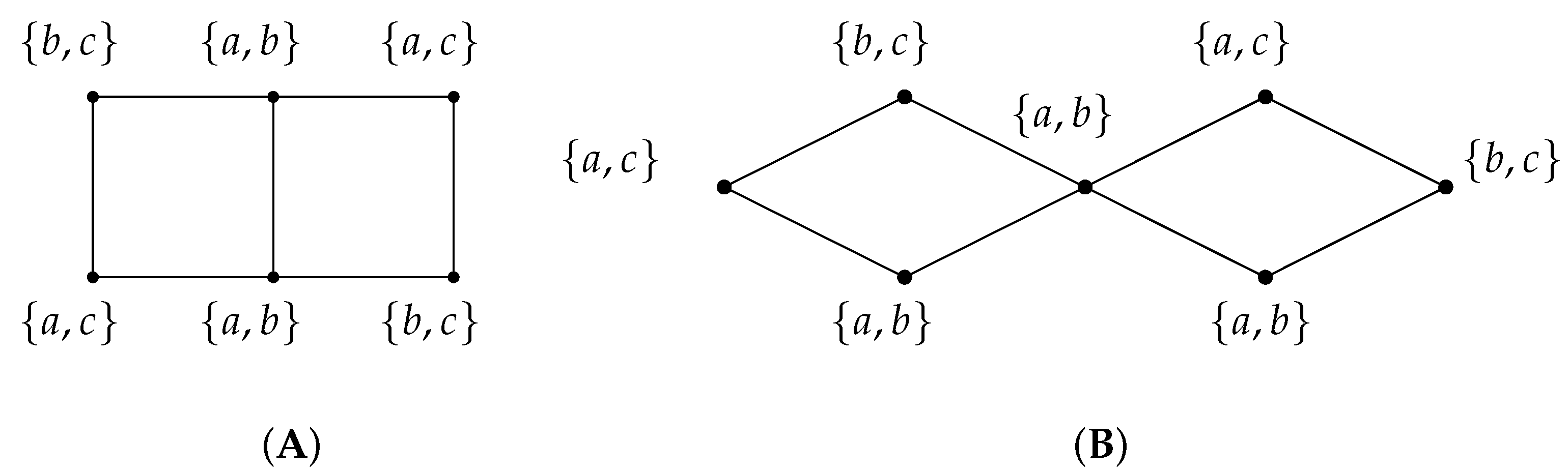
Figure 1A depicts the smallest graph G for which $ch\left(G\right)>\chi \left(G\right)$. In this example, $\chi \left(G\right)=2$, but any choice of colors from the specified lists results in at least one pair of adjacent vertices receiving the same color. By Brooks’ theorem for the choice number [3], $ch\left(G\right)\le \Delta \left(G\right)=3$, and thus $ch\left(G\right)=3$.

The concept of list coloring was introduced in the late 1970s independently by Vizing [4] and by Erdős, Rubin, and Taylor [3]. Ever since, significant work has been carried out (see, e.g., Refs. [5,6,7,8,9,10,11]) to identify classes of chromatic-choosable graphs. List colorings generalize classic proper vertex colorings and admit numerous applications in scheduling, resource management, and optimization where constraints are localized.

One of the most direct applications is in university scheduling and examination timetabling, where each course or event is restricted to certain time slots due to instructor availability or room constraints. These slot limitations translate into list assignments for vertices in a conflict graph, where edges represent overlaps in student enrollments. A successful list coloring guarantees a feasible schedule with no conflicts, and the choice number gives a lower bound on the minimum number of time slots needed under all feasible scenarios [12].

In wireless communications, list coloring arises in frequency assignment problems, where each transmitter can only use specific frequency bands due to regulatory, physical, or environmental constraints. The interference graph models transmitters as vertices, and an edge between two vertices indicates they cannot share the same frequency. Because each transmitter may have its own subset of permitted frequencies, list coloring ensures an interference-free assignment while respecting local constraints. This has profound implications for the design and deployment of modern cellular and wireless networks [13].

Compiler optimization, particularly register allocation, also benefits from list coloring techniques. In register allocation, variables in a program must be assigned to physical CPU registers. When certain variables are constrained to specific registers due to architectural limitations or prior usage, this problem becomes a list coloring instance. Solving it effectively improves runtime performance and reduces memory load, which is especially important in embedded and performance-critical systems [14].

A graph G is said to be chromatic-choosable if $\chi \left(G\right)=ch\left(G\right)$. Cycles, cliques, and trees are examples of chromatic-choosable graphs [3]. For the reader, we list a few well-known results related to this topic for certain classes of graphs, in particular, the complete multipartite and multi-bridge graphs.

Theorem 1

(Erdös, Rubin, and Taylor [3]). The complete k-partite graph $K(2,2,\dots ,2)$ is chromatic-choosable.

Theorem 2

(Galvin [8]). The line graph of any bipartite multigraph is chromatic-choosable.

Theorem 3

(Gravier and Maffray [9]). If $k>2$, then the complete k-partite graph $K(3,3,2,\dots ,2)$ is chromatic-choosable.

We point out here that $K(3,3)$ is not chromatic-choosable since it contains the subgraph in Figure 1 ($K(3,3)$ minus two edges), whose choice number is bigger than 2. Moreover, it was shown in [7] that $K(3,2,2,\dots ,2)$ is chromatic-choosable.

Theorem 4

(Kierstead [15]). Let G denote the complete k-partite graph $K(3,3,3,\dots ,3)$. Then, $ch\left(G\right)=\lceil {\displaystyle \frac{(4k-1)}{3}}\rceil$.

We note here that the previous statement implies that $ch\left(G\right)=k+1$ when $2\le k\le 4$ and $k+1<ch\left(G\right)<{\displaystyle \frac{3k}{2}}$ when $k\ge 5$.

Theorem 5

(Kierstead et al. [16]). Let G denote the complete k-partite graph $K(4,4,4,\dots ,4)$. Then, $ch\left(G\right)=\lceil {\displaystyle \frac{(3k-1)}{2}}\rceil$.

Theorem 6

(Hoffman and Johnson. [1]). Let $G=K(m,n)$ denote a complete bipartite graph. Then,

$$ch\left(G\right)=\left\{\begin{array}{cc}m+1\hfill & \mathit{if}n\ge m^m,\hfill \\ m\hfill & \mathit{if}{(m-1)}^{m-1}-{(m-2)}^{m-1}\le n<m^m,\hfill \\ <m\hfill & \mathrm{otherwise}.\hfill \end{array}\right.$$

Theorem 7

(Enomoto et al. [17]). Let $G_k$ denote the complete k-partite graph $K(4,2,\dots ,2)$. Then,

$$ch\left(G_k\right)=\left\{\begin{array}{cc}k\hfill & ifkisodd,\hfill \\ k+1\hfill & ifkiseven.\hfill \end{array}\right.$$

Theorem 8

(Enomoto et al. [17]). Suppose $k\ge 2$, and let G denote the complete k-partite graph $K(5,2,\dots ,2)$. Then, $ch\left(G\right)=k+1$.

Theorem 9

(Allagan and Johnson [5]). Let G denote the complete k-partite graph $K(6,2,\dots ,2)$. Then, $ch\left(G\right)=k+1$ if $k\ge 2$.

Theorem 10

(Allagan and Johnson [5]). Let G denote the complete k-partite graph $K(m,2,1,\dots ,1)$, $k\ge 3$. Then,

$$ch\left(G\right)=\left\{\begin{array}{cc}k\hfill & {\displaystyle ifm<\frac{k^2+3k}{2},}\hfill \\ k+1\hfill & {\displaystyle ifm\ge k^2.}\hfill \end{array}\right.$$

Theorem 11

(Erdős, Rubin, and Taylor [3]). A connected graph G is 2-choosable if and only if the core of G is $K_1$, an even cycle, or of the form $\theta (2,2,2t)$, where t is a positive integer.

A reminder that the core of a graph G is the graph obtained from G by successively deleting its leaves (vertices of degree 1) until none remain. As such, most results only focus on the potential “core” of some graphs.

The next theorem is arguably the most well-known result by Noel, Reed, and Wu [10] as an attempt to characterize chromatic-choosable graphs (with $\chi >2$); the statement was originally known as Ohba’s conjecture [11].

Theorem 12

(Noel, Reed, and Wu [10]). If $\left|V\right(G\left)\right|\le 2\chi \left(G\right)+1$, then G is chromatic-choosable.

It shows that when the chromatic number is large relative to the order of the graph, the chromatic number is also large enough to equal the choice number. However, there are still several classes of chromatic-choosable graphs whose chromatic numbers are low relative to their orders. For instance, any cycle (of any order) is chromatic-choosable, and Ohba’s theorem only shows that bipartite graphs of an order smaller than 6 are chromatic-choosable.

Theorem 13

(Allagan and Bobga [7]). Suppose $G=\theta (a_1,\dots ,a_l)$ is a multi-bridge graph with $l\ge 3$. G is chromatic-choosable if and only if G contains an odd cycle or G is of the form $\theta (2,2,2t)$, where t is a positive integer.

Theorem 14

(Erdős, Rubin, and Taylor [3]). If G is a connected graph that is neither a complete graph nor an odd cycle, then $ch\left(G\right)\le \Delta \left(G\right)$.

Corollary 1. 

For any graph G, $ch\left(G\right)\le \Delta \left(G\right)+1$.

These results highlight the structural properties of chromatic-choosable graphs and motivate further exploration of graph classes with this property. Our work aims to identify other classes of chromatic-choosable graphs. We begin with chordal graphs, also known as triangulated graphs, in the next section.

3. Choice Number of Chordal Graphs

A graph G is chordal if every cycle of length $l\ge 4$ has a chord. Traditionally, a chord is an edge of G connecting two non-consecutive vertices of the cycle. We found this definition problematic in the context of this paper, which might explain why chordal graphs are often referred to as triangulated graphs. As a subclass of perfect graphs, chordal graphs have at least one simplicial vertex. See [18] for instance. For this reason, we (re)define a chord as an edge of a cycle (of length greater than 3) that contributes to the formation of $K_3$, a triangle, and its removal yields a cycle of length at least 4. 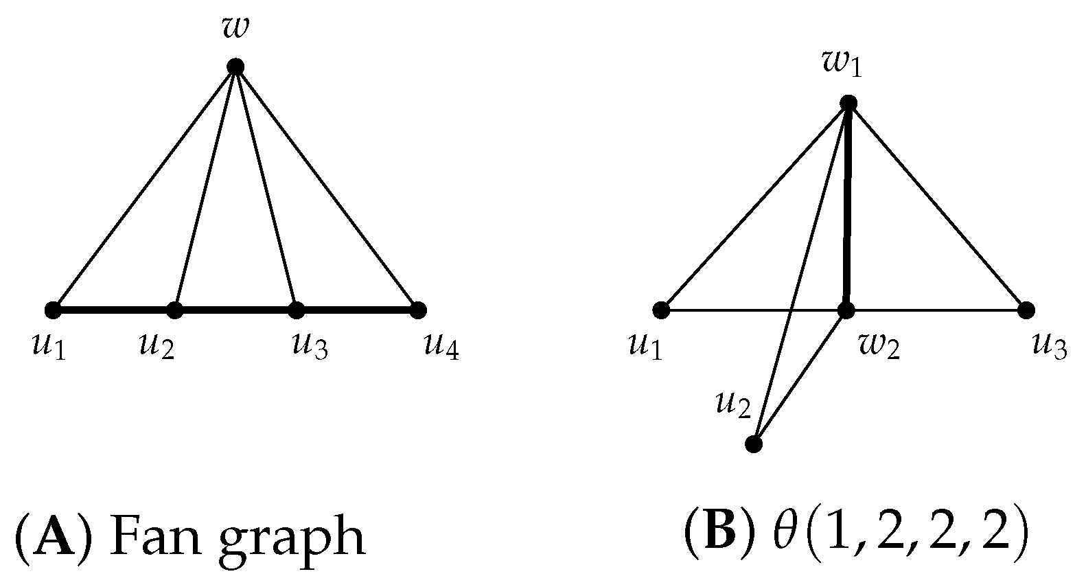Figure 2 shows two well-known chordal graphs. Moreover, the edges $w{u}_2$, $w{u}_3$ are chords in the Fan graph while the edge $w_1{w}_2$ is the only chord in $\theta (1,2,2,2)$.

Theorem 15. 

Chordal graphs are chromatic-choosable.

Proof. 

Let $G=(V,E)$ be a chordal graph with $\chi \left(G\right)=k$. To show that G is k-choosable, we must demonstrate that any list assignment L satisfying $\left|L\right(v\left)\right|\ge k$ for all $v\in V$ permits a proper L-coloring of G.

Since G is a chordal graph, there is a perfect elimination ordering (PEO), denoted as $v_1,v_2,\cdots ,v_n$, of the vertices of G. By definition, in this ordering, for each vertex $v_i$, the set of neighbors of $v_i$ appearing later in the ordering, $\{v_j:j>i\mathrm{and}{v}_j\in N\left(v_i\right)\}$, forms a clique.

We construct a proper L-coloring of G by coloring the vertices in the reverse order of the PEO, starting with $v_n$ and proceeding to $v_1$. At each step i, we assign a color to $v_i$ from its available list $L\left(v_i\right)$ such that the coloring remains proper.

To begin, consider the vertex $v_n$. Since $\left|L\right(v_n\left)\right|\ge k$, assign any color from $L\left(v_n\right)$ to $v_n$. Now, consider $v_{n-1}$. By the properties of the PEO, the only neighbors of $v_{n-1}$ that are already colored are in the clique formed by its higher-index neighbors. Because the size of this clique is at most $k-1$ (since $\chi \left(G\right)=k$), there will always be at least one available color in $L\left(v_{n-1}\right)$ that is distinct from the colors of its neighbors. Assign this color to $v_{n-1}$.

This process continues inductively. At each step i, when coloring $v_i$, its higher-index neighbors form a clique. Thus, the number of colors already used by its neighbors is at most $k-1$. Since $\left|L\right(v_i\left)\right|\ge k$, there is always at least one available color in $L\left(v_i\right)$ that does not conflict with the colors of its neighbors. Assign this color to $v_i$.

By iterating this procedure through the reverse PEO, we construct a proper L-coloring of G. Therefore, $ch\left(G\right)\le k$. Since $\chi \left(G\right)\le ch\left(G\right)$ by definition, it follows that $ch\left(G\right)=\chi \left(G\right)=k$. □

We note here that because chordal graphs admit perfect elimination orderings, any greedy list-coloring strategy can color them successfully if each vertex has a list of size at least $\chi \left(G\right)$. This structure ensures that list coloring does not require more colors than ordinary coloring, a result that is also confirmed in a recent paper by Vasudevan et al. for perfect graphs [19].

A k-tree is a graph constructed from a k-clique by repeatedly adding new vertices, each connected to all vertices of an existing k-clique. It is well-known that k-trees are chordal graphs. Figure 2A,B show two non-isomorphic 2-trees, which are well-known to be chordal graphs.

Corollary 2. 

Every k-tree is $k+1$-choosable for all $k\ge 1$.

Other well-known members of the family of chordal graphs, shown in [2,18,20,21], for instance, include forests, fan graphs, split graphs, interval graphs, k-sun, trivially perfect graphs, threshold graphs, windmill graphs, and strongly chordal graphs.

Remark 1. 

It is tempting to assume that graphs that admit clique separators are likely to be chromatic-choosable. Figure 1 shows two counterexamples: (A) when the clique separator is of size 2 and (B) when the clique separator is of size 1. This demonstrates that the presence of clique separators is not sufficient to guarantee chromatic choosability.

In the next section, we look at chordless graphs, which are graphs whose induced cycles of a length greater than 3 do not have any chord. See Figure 1, for example. Moreover, chordless graphs, which are also known as triangle-free graphs, are not necessarily planar, and they include all bipartite graphs. Our results not only cover some triangle-free graphs (with a neighborhood condition) but also cover graphs that are neither triangulated nor triangle-free; they are known as non-chordal. In general, a non-chordal graph can easily be derived from a chordless graph by adding a sequence of chords to any cycle of length greater than 3, while ensuring that the graph does not become chordal or fully triangulated.

4. Choice Number of Some Chordless and Non-Chordal Graphs

Theorem 16. 

Let $G_1,G_2,\cdots ,G_m$ be the derived subgraphs of a graph G, induced by a set X. Assume that $ch\left(G_i\right)\le ch\left(G_m\right)\le k$ for all $i=1,\cdots ,m-1$. Furthermore, suppose that for every pair of vertices $u,v\in X$, the neighborhoods of u and v outside X in $G_i$ are disjoint, i.e.,

$$N_{G_i\setminus X}\left(u\right)\cap N_{G_i\setminus X}\left(v\right)=\varnothing .$$

Then, the choice number of G satisfies:

$$ch\left(G\right)\le \left\{\begin{array}{cc}k,\hfill & \mathit{if}ch\left(G_i\right)<ch\left(G_m\right)\mathrm{for}\mathrm{all}i<m,\hfill \\ k+1,\hfill & \mathrm{otherwise}.\hfill \end{array}\right.$$

Proof. 

Let L be a list assignment to the vertices of G such that $\left|L\right(v\left)\right|\ge k+1$ for all $v\in V\left(G\right)$. We will show that G has a proper L-coloring under the given conditions.

Begin by properly coloring $G_m$, which is k-choosable by assumption. Since $ch\left(G_m\right)\le k$, there is a proper L-coloring $\varphi$ of $G_m$. For each vertex $u\in X$, let $\varphi \left(u\right)=c_u$ be the color assigned to u by $\varphi$. Let $W_j=N_{G_i\setminus X}\left(u_j\right)$ denote the set of neighbors of $u_j$ in $G_i\setminus X$ for $u_j\in X$. By the hypothesis $N_{G_i\setminus X}\left(u\right)\cap N_{G_i\setminus X}\left(v\right)=\varnothing$ for all $u,v\in X$, the sets $W_j$ are pairwise disjoint.

For each $u_j\in X$, remove the color $c_u=\varphi \left(u_j\right)$ from the list $L\left(w\right)$ of each vertex $w\in W_j$. This operation results in a reduced list assignment $L_1\left(w\right)=L\left(w\right)\setminus \{c_u:u\in X\}$. Since $\left|L\right(w\left)\right|\ge k+1$, it follows that $|L_1\left(w\right)|\ge k$.

Now consider the subgraph $G_i\setminus X$. For each $G_i$, the hypothesis $ch\left(G_i\right)\le k$ ensures that there is a proper $L_1$-coloring of $G_i\setminus X$. Since the sets $W_j$ are pairwise disjoint, no two vertices in different $W_j$ share the same reduced list, ensuring that the proper coloring of each $G_i\setminus X$ is independent of the others. By combining the proper $L_1$-colorings of all $G_i\setminus X$, we obtain a proper L-coloring of G.

If $ch\left(G_i\right)<ch\left(G_m\right)$ for all $i<m$, then G requires at most k colors in total, and $ch\left(G\right)\le k$. If $ch\left(G_i\right)=ch\left(G_m\right)$ for some $i<m$, then the reduction process may require an additional color, and $ch\left(G\right)\le k+1$, hence the result. □

Theorem 17. (Decomposition Theorem).

Let $G_1,G_2,\cdots ,G_m$ be the minimal derived subgraphs of a graph G, induced by the sets $X_1,X_2,\cdots ,X_s$, such that for every $u,v\in X_j$, $N_{G_i\setminus X_j}\left(u\right)\cap N_{G_i\setminus X_j}\left(v\right)=\varnothing$. If $ch\left(G_1\right)\le \dots \le ch\left(G_m\right)\le k$, then

$$ch\left(G\right)\le \left\{\begin{array}{cc}k\hfill & ifch\left(G_i\right)<ch\left(G_m\right)foralli<m,\hfill \\ k+1\hfill & otherwise.\hfill \end{array}\right.$$

Proof. 

Let L be a list assignment to G where $\left|L\right(v\left)\right|\ge k+1$ for all $v\in V\left(G\right)$. We construct a proper L-coloring as follows. First, color $G_m$. Since $ch\left(G_m\right)\le k$, there is a proper coloring ${\varphi }_m$ of $G_m$. Fix this coloring and record the colors assigned to vertices in separators $X_j$ shared between $G_m$ and other subgraphs. Then, adjust the lists for all $G_i\ne G_m$. For each vertex $w\in G_i\setminus X_j$, remove the color ${\varphi }_m\left(u\right)$ from $L\left(w\right)$ if w is adjacent to $u\in X_j$. By the disjoint neighborhood condition, each w is adjacent to at most one $u\in X_j$, so $\left|L\right(w\left)\right|\ge (k+1)-1=k$.

Now, color each remaining subgraph $G_i\ne G_m$. Since $ch\left(G_i\right)\le k$, the reduced list $L^{\prime }$ with $|L^{\prime }\left(v\right)|\ge k$ admits a proper coloring ${\varphi }_i$. The union ${\displaystyle \varphi ={\varphi }_m\cup \bigcup _{i=1}^{m-1}{\varphi }_i}$ defines a proper L-coloring for G. Therefore, one of the following cases holds:

1.

If $ch\left(G_i\right)<ch\left(G_m\right)=k$ for all $i<m$, then $ch\left(G_i\right)\le k-1$. The reduced lists $L^{\prime }$ (size k) suffice for $G_i$, so $ch\left(G\right)\le k$.

2.

If $ch\left(G_i\right)=k$ for some $i<m$, the initial list size $k+1$ ensures $|L^{\prime }\left(v\right)|\ge k$ after adjustments, so $ch\left(G\right)\le k+1$.

Hence, the result. □

We illustrate the decomposition process of Theorem 17 in the next example.

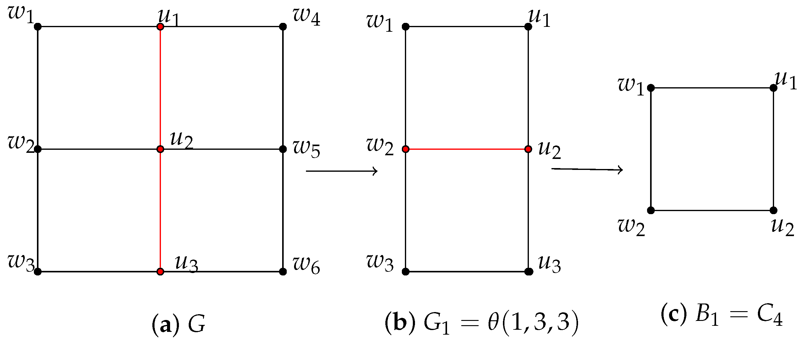
Example 1. 

Choice number of a $3\times 3$ grid: A decomposition.

Consider $G=P_3\square P_3$, the Cartesian product of two paths $P_3$, which forms a $3\times 3$ grid graph with $V\left(G\right)=\{u_1,u_2,u_3,w_1,w_2,w_3,w_4,w_5,w_6\}$. To compute the choice number $ch\left(G\right)$, we illustrate in Figure 3a decomposition of G into derived subgraphs.

Consider the maximal separator, $X_1=\{u_1,u_2,u_3\}$. Note that, for each $u_i\in X_1$, the neighborhood $N_{G\setminus X_1}\left(u_i\right)=\{w_i,w_{i+3}\}$, where $i=1,2,3$, satisfies the condition $N_{G\setminus X_1}\left(u_i\right)\cap N_{G\setminus X_1}\left(u_j\right)=\varnothing$ for $i\ne j$. So, $G\setminus X_1$ produces the derived subgraphs $G_1=G[\{w_1,w_2,w_3\}\cup X_1],G_2=G[\{w_4,w_5,w_6\}\cup X_1]$. For an illustration purpose, we only show the graph $G_1$ in Figure 3 and consider $G_1$ and $G_2$, independently.

Further, we let $X_1^{\prime }=\{w_2,u_2\}$ and $X_2^{\prime }=\{w_5,u_2\}$ be the separators of $G_1$ and $G_2$, respectively. The decomposition process ends with G being divided into four $C_4$’s, denoted by $B_1,B_2,B_3,B_4$.

To compute $ch\left(G\right)$, assign a list L with $\left|L\right(v\left)\right|\ge 3$ for each $v\in V\left(G\right)$. Since $ch\left(B_i\right)=2$, for $i=1,2,3,4$, i.e., $ch\left(B_1\right)\le \dots \le ch\left(B_4\right)$, it follows from Theorem 17 (second assertion) that $ch\left(G\right)\le ch\left(C_4\right)+1=3$. Moreover, because $\theta (1,3,3)\cong G_1\subseteq G$ and $ch\left(G_1\right)>2$, we have $ch\left(G\right)=3$.

Remark 2. 

The previous two theorems give some insight into how to construct and even recognize some classes of chromatic-choosable graphs. So, given a graph G, it suffices to verify that the choice number of one of its components (given the separators’ condition) is bigger than that of any other component. This can be achieved by sufficiently increasing the size of the clique in one of the components either through the graph “join” operation or by connecting any pair of non-adjacent vertices in the case of graphs with even cycles. To see this, add an edge between two non-adjacent vertices for one or both of the two induced cycles $C_4$ in Figure 1B. The resulting graph is chromatic-choosable since its chromatic number is 3. In general, one can add enough chords to cycles (of length greater than 3) of a chordless graph without becoming fully chordal.

Thus, one can form a non-chordal graph that is chromatic-choosable by adding a chord to any cycle of a 2-colorable chordless graph. Moreover, this process can be extended to derive a large class of chromatic-choosable non-chordal graphs, and the next two corollaries, which follow from Theorem 17, affirm their existence.

Corollary 3. 

Suppose $G_1,\dots ,G_m$ are the derived subgraphs of G induced by the sets $X_1,\dots ,X_s$ such that for every $u,v\in X_j$, $N_{G_i\setminus X_j}\left(u\right)\cap N_{G_i\setminus X_j}\left(v\right)=\varnothing$. If $ch\left(G_i\right)=r$, then $r\le ch\left(G\right)\le r+1$.

Corollary 4. 

Suppose $G_1,\dots ,G_m$ are the derived subgraphs of G induced by the sets $X_1,\dots ,X_s$ such that for every $u,v\in X_j$, $N_{G_i\setminus X_j}\left(u\right)\cap N_{G_i\setminus X_j}\left(v\right)=\varnothing$. If for each $i\ne m$, $ch\left(G_i\right)<ch\left(G_m\right)$ and $G_m$ is chromatic-choosable, then G is chromatic-choosable.

5. Estimates of the Choice Number of Some Chordless

Now, we present some results on an upper bound on the choice numbers of the Cartesian product of two graphs, which are special families of chordless graphs. We note that these results apply to non-chordal graphs as well as they are easily formed from these chordless graphs, as mentioned in Remark 2.

For the reader, the Cartesian product of graphs G and H, denoted by $G\square H$, is the graph with vertex set $V\left(G\right)\times V\left(H\right)=\left\{\right(u,v\left)\right|u\in V\left(G\right),v\in V\left(H\right)\}$, where $(u_1,v_1)$ is adjacent to $(u_2,v_2)$ whenever $u_1=u_2$ and $v_1{v}_2\in E\left(H\right)$, or $v_1=v_2$ and $u_1{u}_2\in E\left(G\right)$.

Theorem 18. 

Suppose that $V\left(G\right)=V_1\cup V_2$, $V_1$, and $V_2$ are disjoint and non-empty; $G_i=G\left[V_i\right]$, $i=1,2$; and no vertex in $V_2$ has, in G, more than r neighbors in $V_1$. Then, $ch\left(G\right)\le max\{ch\left(G_1\right),ch\left(G_2\right)+r\}$.

Proof. 

Let $k=max\{ch\left(G_1\right),ch\left(G_2\right)+r\}$ and suppose that L is a list assignment to G such that $\left|L\right(v\left)\right|\ge k$ for all $v\in V\left(G\right)$. Because $k\ge ch\left(G_1\right)$, there is a proper L-coloring $\varphi$ of $G_1$. [More precisely, there is a proper L-restricted-to-$V_1$ coloring of $G_1$.] Define $L^{\prime }$ on $G_2$ by $L^{\prime }\left(u\right)=L\left(u\right)\setminus \left\{\varphi \left(v\right)\right|v\in N_G\left(u\right)\cap V_1\}$. By the hypothesis of the Theorem, $|L^{\prime }\left(u\right)|\ge |L\left(u\right)|-r\ge k-r\ge ch\left(G_2\right)$, for all $u\in V_2$, and, therefore, there is a proper $L^{\prime }$-coloring of $G_2$. Putting this coloring together with $\varphi$, we have a proper L-coloring of G. L was arbitrary, so $ch\left(G\right)\le k$. □

Corollary 5. 

For $n\ge 2$, $ch(H\square P_n)\le ch\left(H\right)+1$.

Proof. 

Let the vertices of $P_n$ be $1,\dots ,n$; let $V_1=V\left(H\right)\times \{1,\dots ,n-1\}$ and $V_2=V\left(H\right)\times \left\{n\right\}$. Then, $V_1$ and $V_2$ are disjoint and non-empty, $V\left(G\right)=V_1\cup V_2$, and every vertex in $V_2$ is adjacent in $G=H\square P_n$ to exactly one vertex in $V_1$. Further, $V_1$ induces $G_1\cong H\square P_{n-1}$ in G, and $V_2$ induces $G_2\cong H$ in G. The conclusion follows from Theorem 18 by induction on n. □

Each of the graphs in the next two corollaries contains the subgraph $H=\theta (1,3,3)$, giving a lower bound of their choice number. The upper bound follows from Corollary 5, giving each result.

Corollary 6. 

For $m\ge 2$, $n\ge 3$, $ch(P_m\square P_n)=3$.

Corollary 7. 

For $r\ge 2$, $n\ge 2$, $ch(C_{2r}\square P_n)=3$.

We note that both Corollary 6 and Corollary 7 follow from a result by Alon and Tarsi, who showed that every bipartite planar graph is 3-choosable [22]. Also, it is worth noting that by Corollary 1, $ch(C_m\square P_n)\le 3$ for all $m\ge 3$. Therefore, $ch(C_m\square P_n)=3$ when m is odd. Together with Corollary 7, we can conclude the next result.

Corollary 8. 

For $m\ge 2$, $n\ge 2$, $ch(C_m\square P_n)=3$.

Corollary 9. 

Suppose that $u\in V\left(H\right)$ has degree $r>0$ in H; then, $ch(G\square H)\le max\{ch\left(G\square (H-u)\right),ch\left(G\right)+r\}$.

Proof. 

$G\square H$ can be formed by connecting $G\square (H-u)$ to a disjoint copy of G in such a way that every vertex of the added G has r neighbors in $G\square (H-u)$. □

Corollary 9 is just a special case of an obvious application of Theorem 18, in which $V(G\square H)=V\left(G\right)\times V\left(H\right)$ is partitioned into $V\left(G\right)\times U_1$ and $V\left(G\right)\times U_2$ for some partition of $V\left(H\right)$ into $U_1\cup U_2$. In Corollary 9, $|U_2|=1$.

We close this section with a more general upper bound on the choice number of the Cartesian product of any two graphs.

Theorem 19. 

$ch(G\square H)\le max\left\{\right|V\left(G\right)|,|V\left(H\right)\left|\right\}$ with equality when $G=H=K_n$.

Proof. 

If G and H are two graphs of order at most n, then $G\square H\subseteq K_n\square K_n$ and $ch(G\square H)\le ch(K_n\square K_n)=ch\left(L\left(K_{n,n}\right)\right)=n$, with the last equality following from Theorem 2. □

Corollary 10. 

If $\left|V\right(G\left)\right|\le n$, then $G\square K_n$ is chromatic-choosable.

6. Conclusions

The results presented in this paper provide new insights into the relationship between the structure of a graph and its choice number, particularly for chordal, chordless, and some non-chordal graphs. Together, the corollaries and the example illustrate a connection between chromatic-choosability and graph decompositions, offering new tools to identify classes of chromatic-choosable graphs that are chordless or non-chordal. The question of whether there might be non-chordal graphs that are 2-choosable, thus chromatic-choosable, was answered affirmatively by Erdös et al. [3] when they characterized all 2-choosable graphs, mainly that every component of such graphs must be 2-choosable. We hope that the results presented here will help further characterize 3-choosable graphs given some earlier work in this respect by Alon et al. [22] when they showed that every bipartite planar graph is 3-choosable; our results make no distinctions between planar and non-planar graphs as every bipartite graph is chordless and non-chordal graphs include all multipartite graphs with 3 or more parts. Finally, we observe that the bound of Theorem 17 is tight for planar graphs, as Voigt and a few other researchers [23,24,25] have found some examples of planar triangle-free graphs (having more than two odd holes) that are not 3-choosable.