Abstract
It is vital to study the stability of power systems under small perturbations to prevent blackouts. This study presents a load-shedding strategy that has been incorporated within the swing equation to reduce instability and delay the onset of chaotic dynamics. The objective of this study was to identify the minimal load reductions required after disturbances to maintain the frequency above a critical value. Analytical techniques such as eigenvalue analysis and perturbation methods can also be supported with numerical simulations using bifurcation diagrams, Lyapunov exponents, and the Simulink model. When compared to the conventional stepwise load-shedding method, the proposed approach allows for dynamic adjustments and presents a 49% increase in stable regions and a 45% reduction in recovery time. Performance was also analysed under different damping, inertia, and load scenarios. These results suggest that the strategy demonstrated in this research provides a robust and computationally practical solution for modern power system applications.
MSC:
37M99
1. Introduction
Analysing the stability of nonlinear systems is crucial, particularly under sudden minute disturbances that may cause blackouts and failures within the system [,]. An important aspect of stability depends on maintaining the frequency of the system within the given operational limits, which can undergo disruptions caused by sudden disparities between demand and generation []. To reduce such adverse effects, control approaches can be applied to sustain the stability of the frequency during short-term events.
The swing equation, which is a second-order differential equation, is used to model the dynamical behaviour of the rotor in synchronous machines [,]. Numerical solutions have been traditionally employed to study the complex behaviours of nonlinear systems []. Recent studies have used analytical techniques to provide a deeper insight into stability boundaries under various conditions [,].
Previous studies have shown the evolution of load-shedding techniques from static, rule-based schemes to more adaptive control mechanisms []. Conventional techniques such as under-frequency load shedding (UFLS) are simple but mostly result in over-shedding or under-shedding due to fixed thresholds [,]. Furthermore, such methods lack the ability to generate real-time responses and fail to consider the impact of perturbations. These limitations have influenced the development of data-driven strategies that can consider shedding actions based on present power grid conditions [,,,].
While a wide range of modern techniques exist, from voltage indicators to AI-driven and game-theoretic models, many researchers consider load shedding to be an external corrective action, disconnected from the governing equations of system dynamics.
This study addresses this gap by proposing a control-based load-shedding technique incorporated directly within the swing equation. The main aim of this study is to analytically determine the minimal load reduction that is necessary to stabilise the system after small disturbances, as well as examine the impact of the inclusion of the shedding term to mitigate chaos. By modifying the swing equation’s damping characteristics by including a load-shedding term, the method provides insight into the real-time impact of control on nonlinear system dynamics.
The objectives of the study include deriving the analytical expression for the swing equation with the incorporation of the load-shedding term and assessing system stability using eigenvalue analysis, Lyapunov exponents, bifurcation diagrams, and perturbation techniques. This study also compares the proposed method against the conventional load-shedding approach using both analytical and numerical methods. It examines the robustness of the method under different parameters and validates the approach using Matlab Simulink.
2. Literature Review
The analysis of stability in nonlinear systems during small and sudden disturbances has become an important area of research, especially within the context of increasingly complex power grids. Load shedding is one of the most popular adopted emergency control approaches that can be used to prevent system collapse and maintain the frequency stability of systems [].
A vital tool in modelling such intricate systems is the swing equation, which describes the rotor motion of synchronous generators. It is a second-order differential equation that is used to study stable regions during perturbations [,]. Solving the swing equation analytically can be challenging due to its nonlinearity; early studies relied solely on numerical methods. However, new strategies have examined the potential of analytical methods, providing a deeper understanding of system stability regions [,]. For example, Cartesian coordinates’ reformulations have aided in analytical approximations that can be compared to traditional numerical methods [], while the ZIP load models have improved for use in real-world applications through a consideration of certain components—namely current, impedance, and power [].
Conventional load-shedding approaches, such as under-frequency load shedding (UFLS), are used in many sectors due to their simplicity. These strategies detach the previously determined loads when the frequency thresholds are breached []. Although they are easy to implement, they lack adaptability and are reactive. UFLS does not consider the impact of perturbations and real-time conditions; it often results in insufficient or excessive load shedding within the system, which, in turn, increases instability.
To improve on the UFLS method, voltage indicator-based strategies can be used through an assessment of a system’s voltage margin and estimating how much load can be shed before the system cascades to instability []. These techniques are more location-specific and responsive. However, their effectiveness is limited to voltage-driven stability issues and, hence, may not perform well in systems where frequency dynamics are predominant.
Strategies based on machine learning techniques have become widely used in recent years to forecast optimal load shedding decisions in real time [,]. Using historical data and simulations, these approaches can predict disturbances and trigger control methods. However, these machine learning models depend on large, high-quality datasets, and researchers might find it challenging to use them to generalise across different grid topologies. They also lack analytical traceability and interpretability.
Considering game-theory approaches to modelling power grids, one can consider them to be cooperative environments, where different components and agents—like the generators, regions, or even consumers—decide on the load-shedding strategy based on mutual understanding []. These methods can provide equilibrium-based shedding plans for grids, reducing instability. However, they involve complex optimisation problems and generally require strong assumptions about agents, which may be challenging in physical system spaces.
Hence, this study introduces a control-embedded load-shedding approach where the shedding term is included in the swing equation. This method models load shedding as a part of the system’s dynamics but provides an analytical expression for natural frequency, the damping ratio, and system stability after they have been modified through the control. Hence, this approach offers both interpretability and predictive power whilst bridging the gap between theoretical study and real-time applications.
Table 1 compares different load-shedding approaches to aid our understanding of the importance of the approach suggested in this study.

Table 1.
Comparison of load-shedding strategies with the proposed approach.
3. Methodology
The equation analysing the rotor’s motion of the machine, including a damping term, is given by [,].
where the following applies:
= constant angular velocity;
H = inertia;
D = damping;
= mechanical power;
= voltage of machine;
= transient reactance;
= voltage of busbar system;
= phase of busbar system;
and magnitudes are assumed to be small.
Here, we derive an equation for system frequency, , which relates to the time derivative of the rotor angle:
where is the rated system frequency.
Then, we differentiate both sides with respect to time:
Then, we substitute into swing Equation (1) the following:
This equation describes how the frequency, , evolves over time based on power input, electrical power transfer, and damping.
The aim is to make sure that the system frequency remains above the minimum threshold to reduce unstable regions. During a small perturbation, the electrical power, , might drop because of faults in the grids. This might adversely affect nonlinear systems.
To study the effect of these perturbations, it is necessary to approximate using a first-order Taylor expansion around the steady-state condition :
Load shedding is introduced to alter , reducing the effective electrical power. Let be the load shed, such that
Then, we expand in the swing equation:
The load-shedding objective is to determine , such that
The load-shedding term, , was introduced into the swing equation to evaluate its effect on system stability []. Load shedding was triggered when the rotor angle deviation exceeded a defined threshold. At each time step, if this threshold was breached, the system shed a fixed percentage of electrical power. The values tested were 0.05, 0.1, and 1.2 per unit (pu). The values were carefully selected to represent light, moderate, and high levels of load reduction, respectively, and were chosen to examine how increasing control effort influences system dynamics. The effect of load shedding was studied by comparing the delay in chaotic parts in bifurcation diagrams and was validated using Lyapunov exponents.
3.1. Analytical Work
3.1.1. Derivation of the Stability Equation with Load Shedding
The modified swing equation including load shedding is given by
Expanding :
Then, we consider small deviations around the equilibrium , leading to the following linearised system:
This equation follows the form of a standard second-order differential equation:
The natural frequency is
The damping ratio is modified due to the incorporation of load shedding :
The characteristic equation was
Then, we solve for the eigenvalues:
The eigenvalues were plotted for different values of , depicting a leftward shift as load shedding increased. This confirmed that higher values enhanced system damping and reduced oscillations, leading to delayed chaos within the system.
3.1.2. Perturbation Analysis
The standard swing equation, which governs the rotor dynamics of a synchronous machine including damping and electrical power terms, is given by [], as follows:
where the following applies:
- is the mechanical power input.
- is the electrical power output.
To enhance stability, we introduce the load-shedding term within Equation :
where
Equation (23) shows a small perturbation effect on the load-shedding term, where —this depicts the initial state and is assumed to be very small.
Then, we expand using a first-order Taylor series approximation:
By introducing perturbations in rotor angle,
Next, with consideration of the transformations being allowed,
Then, Equation (26) becomes
Substituting Equations (26)–(28) into Equations (1)–(3), we derive the modified swing equation with excitation:
where
Thus, Equation (30) reduces to
Initially, the focus of the analysis is on primary resonance. To study this, multiple scales are used to find a uniform solution for Equation (32). A small dimensionless parameter, , is introduced to account for the effects of damping, nonlinearities, and the excitation frequency, which occur in a specific order.
We let
and
Then, the final equation from the swing equation derivation above has the following coefficients:
Furthermore, we consider the equation with the detuning parameter ,
to allow for the derived final swing Equation (32) to be rewritten as
The solution to the above equation is of the following form:
where is a fast scale describing motions of frequencies, and and are slow scales describing amplitude variation [].
The first derivative of this equation is as follows:
The second derivative is as follows:
where
Equation (39) can be rewritten as follows:
Finding the first derivative with respect to t for Equation (43) and substituting Equation (40) gives
Differentiating for the second derivative with respect to t for Equation (43) and substituting Equation (41) gives
Substituting Equations (43)–(45) into Equation (32) and comparing coefficients of gives
From Equations (46)–(48), it can be seen that the parametric terms do not have key effects on the system. Hence, only the external forcing term remains [,].
The solution to Equation (46) is of the following form:
where A is an undetermined function. Given that
by integration,
With Equation (49) substituted into (47),
With the brackets expanded,
Due to and
Substituting into the equation and rearranging leads to
where is the complex conjugate. In this equation, , to avoid secular terms, ; hence, . Replacing Equation (46) into (49) and simplifying, we obtain
which is also echoed in [,].
Replacing Equations (49) and (55) into Equation (48), we obtain
where
Expressing A in polar form, we obtain
Substituting Equation (57) into Equation (56) gives
Equation (57) can also be written in the following form:
Substituting A and its conjugate into Equation (49) leads to
Similarly, replacing into Equation (55) gives
Substituting the above derivations for and in Equation (39) to obtain the second approximation, we obtain
Setting and letting “a” be the perturbation parameter, using Equation (63), Equation (28) may be rewritten as
with defined as the drift term; because of its quadratic nonlinearity, the oscillatory motion is not centred, as also seen in [,].
To understand the character of Equations (58) and (59), fixed points are found in alignment with to reduce to
Squaring and adding Equations (65) and (66) will give
The analytical results are compared with the numerical simulations for primary resonance when = 8.61 with the load-shedding term. The Runge–Kutta fourth-order and Newton–Raphson methods were used for the simulation perturbation analysis and compared with the numerical results, as shown in Figure 1. It can be seen that the Newton–Raphson method yields a better approximation of the numerical solution. The calculated numerical error of the Runge–Kutta method versus the Newton–Raphson technique compared to the actual numerical solution error was 0.04192 and 0.02314, respectively, ensuring that the Newton–Raphson method is a suitable fit because of its small error value.
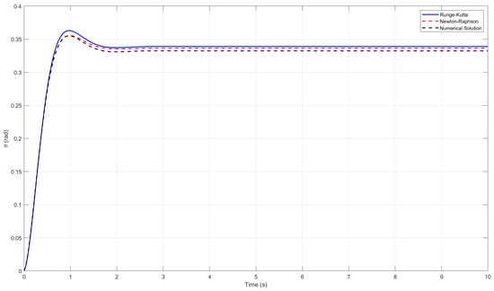
Figure 1.
Perturbed solution employing Runge–Kutta and Newton–Raphson algorithms in comparison to numerical simulations for the case of primary resonance in the phase plane and time history for = 8.61 .
The bifurcation diagrams are generated by incrementing the forcing parameter, r, while continuing the time integration of the system at each step [,,]. For each value of r, the maximum amplitude of the oscillatory solution is computed and plotted against r. This process reveals how the system’s behaviour evolves as the forcing parameter is varied, showing transitions between periodic states, chaotic states, and even intermittency. r is considered as follows:
The transformed swing equation was solved in Matlab using the fourth-order Runge–Kutta method for numerical accuracy, including the load-shedding term. As the load shedding increased, the minimal point was found where the chaos was delayed for the system in hand.
The conventional scheme bifurcation diagrams were also produced, where the system was solved in a step-by-step manner. The findings showed that the chaos happened earlier in comparison to when the load-shedding term was introduced into the system.
The Lyapunov exponents were produced to quantify the system’s sensitivity to initial conditions []. A positive Lyapunov exponent shows chaos, while a negative exponent shows stability. As load-shedding values are increased, the Lyapunov exponents shifted towards negative values, confirming reduced chaos. The chaos began later in comparison with the case with no load shedding in the system.
A conventional load-shedding method was used for comparison, where the electric power was performed in a stepwise process with time intervals []. Instead of shedding the load only when instability occurred, fixed shedding steps were introduced every 5 s. This method led to chaos occurring earlier, showing that the load-shedding strategy studied here is more effective in delaying chaos. Hence, it is important to consider the effect of the parameters on the system [].
The model assumes a single-machine infinite busbar system with constant parameters, such as damping, inertia, and generator voltage. These simplifications are needed to derive analytical results and gain insight into stability mechanisms; while the real system has more complex variables and reactive power dynamics, and even different topologies, these assumptions are valid for studying local generator behaviour during short-term transients. Hence, future research can extend this approach to complex power grid structures and observe the stability behaviour when more parameters are considered.
4. Results
4.1. Representation of the Analytical Work
Figure 2 shows the eigenvalues calculated for the swing equation without any load-shedding terms. For negative damping (), the eigenvalues have positive real parts, which means the system experiences exponentially increasing oscillations. This indicates that the system is unstable, and disturbances are growing.
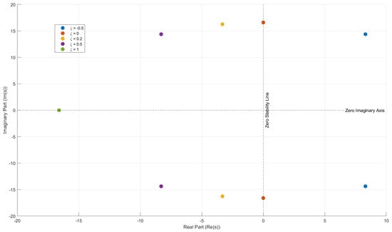
Figure 2.
Eigenvalues obtained from the swing equation without any load-shedding term when = 8.61 .
When the damping ratio is zero, the eigenvalues lie purely on the imaginary axis. That is, the system exhibits continuous oscillations without decaying in the system.
For under-damped cases (0 < < 1), such as = 0.2 and = 0.5, the eigenvalues shift leftward but still have imaginary components in the values. This means the system oscillates but gradually settles down after some time. The closer the damping ratio is to 1, the better, as decaying occurs quickly.
For critical damping ( = 1), the eigenvalues become real and negative, meaning the system returns to equilibrium without oscillations. This is the ideal damping scenario desired by researchers and engineers in the sector.
Figure 3 depicts the eigenvalues obtained for the swing equation with the load-shedding term. For zero load shedding, the eigenvalues remain close to the imaginary axis.
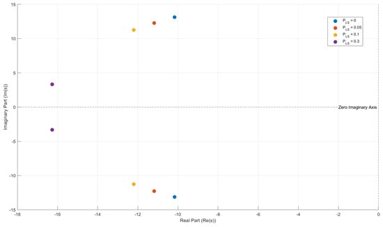
Figure 3.
Eigenvalues obtained from the swing equation with load-shedding term when = 8.61 .
As load shedding is increased, the eigenvalues shift leftward, signifying improved damping and enhanced stability. For higher load-shedding values, the eigenvalues move further into the left-half plane, reducing the imaginary component.
4.2. Representation for the Primary Resonance
The bifurcation diagrams shown in Figure 4 are produced for the swing equation with the load-shedding term. The swing equation without any load shedding shows early chaotic behaviour []. As the load-shedding term is incorporated within the system, a slight shift can be seen in the diagrams.
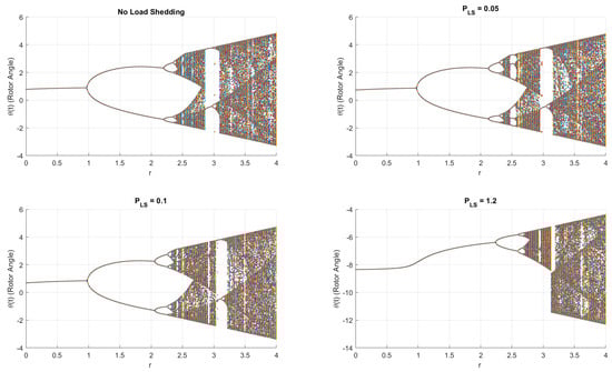
Figure 4.
Bifurcation diagrams when the load-shedding terms are increasing in the scheme analysed in this study for primary resonance at = 8.61 .
For higher load-shedding values ( = 1.2), the bifurcation diagram shows a nearly entirely stable regime, where chaotic oscillations are reduced. Instead of multiple bifurcation branches, the system exhibits a single, stable trajectory, confirming that load shedding helps maintain predictable frequency responses. However, excessive load shedding may over-stabilise the system, potentially making it slower to adapt to transient changes. When are greater than 1.2, the system exhibits chaotic response, showing that, when = 1.2, the system attains a delay in chaos and stays stable for a long time.
Figure 5 shows the Lyapunov exponents for the bifurcation diagrams obtained when using the load-shedding method described above. Without load shedding, positive Lyapunov exponents are observed, confirming that the system exhibits dependence on initial conditions. As increases, the Lyapunov exponents shift to negative values, confirming that load shedding effectively mitigates chaotic dynamics and ensures predictable system behaviour. When = 0, the system enters chaos when r = 2.2 []. However, when the load-shedding term is increased to 0.05, the chaos begins at r = 2.3. As the load-shedding term is increased to 1.2, it can be observed that the chaos begins at r = 2.72, showing that the strategy considered has delayed the system from entering an unstable region.
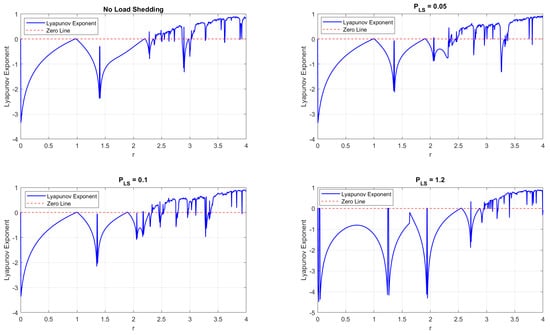
Figure 5.
Lyapunov exponents for the primary resonance for the load-shedding scheme when = 8.61 .
The basins of attraction in Figure 6 show the regions of initial conditions that lead to stable operation. The red and the green regions depict the stable parts. Without load shedding, the stable basin is relatively small, meaning that even minor disturbances can drive the system into instability. However, as increases, the stable basin expands, confirming that load shedding enhances the ability of the system to return to equilibrium after disturbances. The stability area increases; that is, there is an increase in the number of pixels, demonstrating a substantial improvement in the system’s dynamic response. These results reinforce the idea that load shedding should be dynamically optimised to maximise stability without an excessive energy loss.
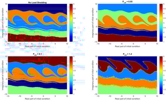
Figure 6.
Basins of attractions with load-shedding term within the swing equation for primary resonance when = 8.61 .
4.3. Representation for the Conventional Scheme
The bifurcation diagrams depicted in Figure 7 for the conventional load-shedding scheme highlight a key difference in stability behaviour compared to the adaptive load-shedding method. In the conventional approach, where load shedding is triggered at fixed frequency thresholds, the system still exhibits chaotic oscillations but with an earlier onset of instability. The bifurcation diagram shows chaotic behaviour occurring at lower parameter values of r, meaning that the system enters an unstable regime much sooner. This suggests that the traditional stepwise load-shedding mechanism does not effectively delay chaos.
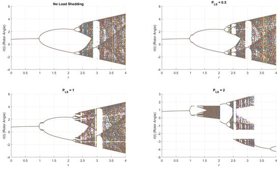
Figure 7.
Bifurcation diagrams when the load-shedding terms are increasing using the conventional scheme when = 8.61 .
Compared to the load-shedding approach discussed in this study—which gradually shifts bifurcations further into the stability region—the conventional scheme lacks control, resulting in over-shedding or under-shedding in electric power circuits, both of which contribute to chaotic oscillations. Additionally, instead of a smooth transition into stability, the bifurcation diagram for the conventional scheme exhibits abrupt jumps between periodic and chaotic behaviour, further confirming the inefficiency of a fixed threshold approach in reducing instability.
4.4. Representation for the Subharmonic Resonance
Figure 8 shows bifurcation diagrams for the subharmonic resonance when = 19.375 . In the swing equation, a load-shedding term is introduced and the output is analysed to identify chaotic behaviour.
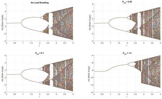
Figure 8.
Bifurcation diagrams when the load-shedding terms are increasing in the scheme analysed in this study for subharmonic resonance when = 19.375 .
The first diagram shows the dynamical behaviour when there is no load-shedding term in the swing Equation [,]. At around r = 2.15, the chaotic behaviour can be seen. When the load-shedding term is = 0.05, chaos can only be observed at r = 2.2. As the load-shedding term increases to 1.2, the system cascades to chaos at r = 2.47. This shows that chaos is delayed when the load-shedding term is incremented slightly, validating the results of the controlled load-shedding scheme discussed in this study.
The basins of attraction in Figure 9 depict the regions of initial conditions and stability for subharmonic resonance. The red and the green sections show the stable regions. Without load shedding, the stable basin is relatively small; however, as the load-shedding term increases, the stable basin expands, confirming that load shedding enhances equilibrium.
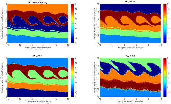
Figure 9.
Basins of attractions with load-shedding term within the swing equation when = 19.375 .
Figure 10 shows the relationship between load shedding and an increase in the stability region for both primary resonance when = 8.61 and subharmonic resonance when = 19.375 . It can be observed that the stability increases as load shedding is incremented. At = 1.2, the stability region increases to a maximum by 49.21% for primary resonance and 45.34 % for subharmonic resonance. The results validate the bifurcation diagrams and Lyapunov exponents, confirming that the load-shedding term helps to delay chaotic oscillations.
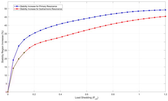
Figure 10.
Increase in stability as the load-shedding term is incremented for primary resonance when = 8.61 and subharmonic resonance when = 19.375 .
4.5. Load Shedding in the Matlab Simulink Model
Figure 11 illustrates a generic block diagram of the power system with integrated load-shedding control. The generator block represents the mechanical power input, , which drives the system. The power system block models the swing dynamics and includes the system’s inertia, H, damping, D, and the electrical power output, , reflecting the classical swing equation formulation. The output of this block is the angle of the rotor, , which is continuously monitored. The control block receives and its derivative as inputs and calculates the appropriate load-shedding action, which is then fed back into the power system. This structure captures the implementation of the modified swing equation with control, such as Equation (13), where the damping is effectively improved through the inclusion of the load-shedding term.
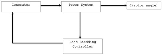
Figure 11.
Conceptual schematic of the power system integrated with the proposed load-shedding control loop.
The Simulink model shown in Figure 12 depicts the swing equation model with the load-shedding term. To analyse the behaviour around the primary resonance, = 7.5 was chosen, as it is a value closer to the primary resonance, and similar dynamical observations can be seen. To consider a value closer to subharmonic resonance, = 18.9 was selected.
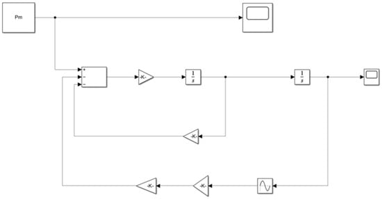
Figure 12.
Simulink model of the swing equation with the load-shedding term when = 7.5 .
The Poincaré maps in Figure 13 were obtained from the Simulink model above to show the delay in chaos due to the introduction of the load-shedding term. The first map depicts the behaviour of the system when there is no load-shedding term and when = 7.5 . When a load-shedding term of 1.2 pu is added to the system, a clear delay in chaos can be seen. For the ‘no load shedding’ map, chaotic behaviour appears when with widely scattered points. In contrast, in the map with load shedding, chaos can be observed around . This demonstrates that introducing the load-shedding term again delayed the chaotic behaviour, enhancing the reliability of the system.
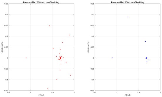
Figure 13.
Poincaré maps from the Simulink model showing the delay in chaos after the load-shedding term is included for = 7.5 .
Figure 14 shows the Poincaré maps with and without the load-shedding term when = 18.9 . Without the load-shedding term, chaos begins when ; when the load-shedding term is included, chaos appears when , with few points on the map. This validates the importance of the load-shedding approach for the swing equation.
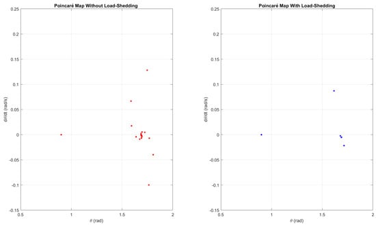
Figure 14.
Poincaré maps from the Simulink model showing the delay in chaos after the load-shedding term is included for = 18.9 .
To validate the results found, time-series data were obtained for the rotor speed.
Figure 15 depicts the time-series and phase portraits of the rotor speed in the swing equation, comparing the system’s behaviour with and without load shedding when = 7.5 , which is closer to the primary resonance value. In the case without load shedding, irregular oscillations occur for an extended period before gradually settling into a stable oscillatory pattern. This indicates that disturbances persist longer within the system. Through the phase portraits, it can be observed that, with load shedding, the system enters a stable region with fewer spirals in comparison with the case without the load-shedding term. Hence, we show that the system enters stability quickly when a load-shedding term is introduced into the equation.
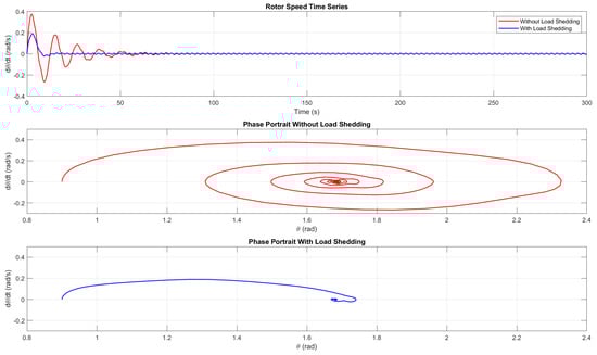
Figure 15.
Time-series and phase portraits for the rotor speed with and without load shedding for = 7.5 .
With the load-shedding approach, the rotor speed reaches stable oscillations much earlier. The additional damping effect introduced by load shedding effectively reduces the amplitude of oscillations and suppresses chaotic behaviour, leading to faster stabilisation. This ensures the importance of the inclusion of the load-shedding strategy to reduce fluctuations.
Figure 16 shows the behaviour of the system when an value is considered, which is closer to the subharmonic resonance. At = 18.9 , the time-series and the corresponding phase portraits with and without the load-shedding term are compared. It also validates the importance of the load-shedding term and how it delays the chaos occurring within the system.
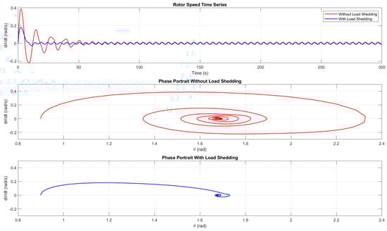
Figure 16.
Time-series and phase portraits for the rotor speed with and without load shedding for = 18.9 .
Table 2 compares the proposed load-shedding approach and the conventional (UFLS) method using performance metrics. The proposed technique delays the onset of chaos, increasing the critical bifurcation, showing a 26.5% improvement. It also expands the stability region with a 104% relative increase. Additionally, the system recovery time is nearly halved, depicting a 45% quicker return to a steady state. Unlike the conventional method, which disconnects load at fixed intervals, the approach discussed in this study only sheds load when instability is found, which in turn reduces the power cuts. The Lyapunov exponent shift also indicates stronger damping and improved resilience within the system. These findings quantitatively confirm and validate that the proposed strategy offers more effective control mechanisms for maintaining power system stability.
Table 2.
Quantitative performance comparison: proposed method vs. conventional (UFLS) method.
4.6. Sensitivity Analysis of the System’s Parameters
Studying how key system parameters affect power system stability is vital for analysing the robustness of control strategies. A sensitivity analysis was carried out to examine the influence of the parameters of damping and inertia on the dynamics of the swing equation when the swing equation with the load-shedding term was considered. By varying each parameter, phase portraits were plotted and analysed to observe the system’s behaviour. These findings are particularly relevant for real-world implementation, where grid parameters can also change to different topologies and conditions.
Figure 17 shows the phase portraits when the damping values were increased in the swing equation with the load-shedding term. As the value increased by 0.5, the system quickly converged to an equilibrium point, indicating improved system stability. This confirms the expected stabilising effect of damping and demonstrates that the proposed load-shedding strategy maintains its effectiveness even when intrinsic system damping is low—a common scenario in renewable-heavy grids.
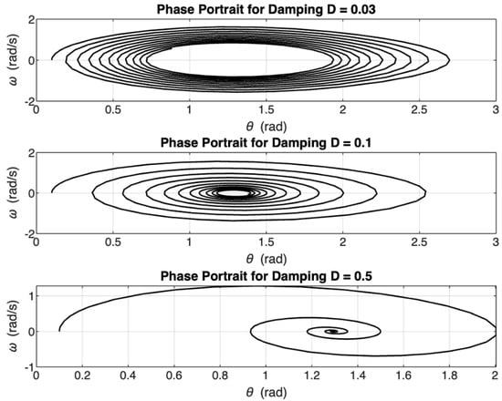
Figure 17.
Phase portraits when damping is altered when the load-shedding term is included in the swing equation for = 8.61 .
Figure 18 shows the phase portraits of the swing equation with the load-shedding term when the inertia is incremented. As inertia increases, the phase portraits become more compact and the system transitions more slowly but steadily toward equilibrium. Additionally, the proposed load-shedding strategy remains effective across all inertia levels, helping compensate for the reduced natural stability in low-inertia systems.
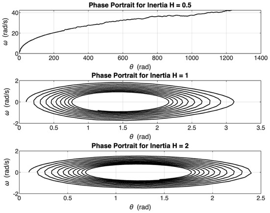
Figure 18.
Phase portraits when inertia is altered when the load-shedding term is included in the swing equation for = 8.61 .
4.7. Load Disturbance
To further examine the effectiveness of the proposed load-shedding technique, phase portraits were employed to study the system’s dynamics behaviour under a sudden load disturbance. A 25% load increase was applied to simulate a realistic disturbance scenario.
Figure 19 shows the phase portraits when a sudden load disturbance was introduced to the swing equation with the load-shedding term. In the graph, where no control is applied, the trajectory forms wider, loosely spiralling loops, indicating sustained oscillations and slow convergence toward equilibrium. This reflects the system’s reduced ability to self-stabilise after a small perturbation. In the graph with an active load-shedding control—as proposed here—the phase trajectory is noticeably tighter and converges more quickly to the origin, showing improved damping and faster stability recovery. The reduced phase space figure highlights how the embedded control strategy effectively suppresses the disturbance and prevents unstable behaviour.
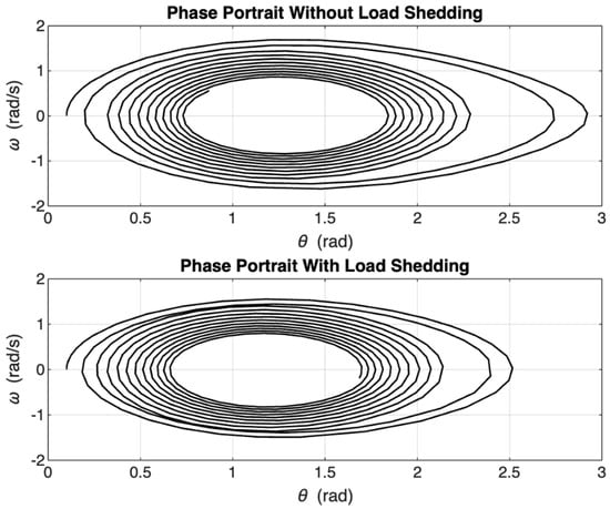
Figure 19.
Phase portraits when sudden disturbance is introduced when the load-shedding term is included in the swing equation for = 8.61 .
5. Discussion
The results of this study show that the optimised load-shedding method plays a vital role in improving the stability of the system reducing chaotic oscillations. The eigenvalues confirm that increasing the values enhances damping and shifts the eigenvalues to the left half-plane, ensuring a better and more stable response. These results are similar to those of previous research that has been performed on power system stability, where damping mechanisms have reduced system collapse. The quantitative analysis of bifurcations and Lyapunov exponents in this study provides deeper insight and understanding of the swing equation system, showing an influence of the load-shedding method, which in turn delays chaotic oscillations.
The proposed approach is compared to the traditional conventional under-frequency load-shedding scheme, which applies stepwise disconnections based on defined frequency values. This conventional method often results in under-shedding or over-shedding because it does not severity of the disturbances. In contrast, the load-shedding method discussed here ensures that only a minimum amount of load is shed to gain stability back, preserving system integrity and continuity of service. This aligns with the direction of modern smart grid technologies, which rely on adaptability and real-time control strategies.
In a practical context, the proposed method can be integrated into real-world nonlinear systems to enhance operational reliability. One of the main key advantages is its potential to reduce or prevent blackouts in large interconnected power circuits by providing timely control actions during perturbations. This approach also offers economic benefits by decreasing unnecessary disconnections of consumers, thereby minimising financial strain on households and industries. As blackouts result in significant economic losses, a method that preserves stability with minimal load shedding can improve both system performance and customer satisfaction.
To validate the practical application of the method, a Matlab R2023a Simulink model was developed, simulating the key parts of physical power systems, including the load and generators. The results from the Simulink showed similar behaviour to the analytical and numerical findings, reinforcing the validity of the proposed approach. The block-based implementation allows the method to be tested in a controlled environment and potentially extend it to hardware-in-the-loop testing in the future.
While the Simulink model captures the dynamic behaviour of the swing equation, it does not explicitly include the full equivalent circuit of the power system. Hence, the main limitation is related to the network topology, line impedances, and generator parameters. These factors influence the transient responses of the power systems. However, the swing equation model includes electrical components such as generator reactance, bus voltage, and power angle; these reflect the system’s electric characteristics. Future research could focus on incorporating this into multi-machine models or IEEE benchmark test systems to provide a more detailed and realistic representation of the system’s response.
Another important insight from this study is that excessive load shedding may lead to adverse effects. If the shedding level surpasses a certain threshold value, the system goes into unstable regions or will be slow to recover from disturbances. The result indicates that an optimal range for load shedding exists, where stability balance is maintained. Over-shedding may slow down recovery, while under-shedding may not be enough to prevent instability.
Within the context of the computational aspect, this method is highly efficient. The control logic considered is simple; that is, it monitors the system’s rotor angle or frequency and activates a proportional load-shedding response when the required thresholds are exceeded. As iterative measures are not used in the model involved, the approach is lightweight and suitable for real-time applications. It can be included on standard supervisory control and data acquisition or phasor measurement unit-based infrastructure without requiring complex computing systems.
Although the current model assumes fixed parameters and does not include real-time measurement feedback, the strategy is compatible with the future integration of AI-driven and machine learning techniques. Such incorporation could enable the system to predict instabilities and adapt shedding approaches in real time. This is particularly relevant, as power systems increasingly rely on renewable energy sources, which have uncertainty and greater variability. By embedding the control within the power system dynamics, the proposed approach lays the groundwork for a system that maintains frequency stability even under complex conditions.
6. Future Research
Although this study used parameter values that reflect real-world generators and similar grid conditions, no actual grid data were used. Incorporating IEEE benchmark systems (e.g., 9-bus or 39-bus models) and using real operation data would further strengthen the practical relevance of the results. Future work can focus on validating the method using real-time simulations and hardware-in-the-loop (HIL) environments.
Future improvements may also involve incorporating the control-embedded technique with machine learning methods to create predictive load-shedding responses. This will be helpful in modern power grids with high renewable penetration, where system inertia is low, and fast control is essential. Hence, extending the complexity of the model and validating it across real-world scenarios will be crucial for real-time infrastructures and the development of smart grids.
7. Conclusions
This study introduced a mathematically involved, control-embedded load-shedding approach that improves frequency stability in nonlinear power systems by modifying the swing equation. The main contribution of the work is the inclusion of the load-shedding term directly into the swing equation; this allows the control mechanism to operate as an internal dynamic and not as an external correction. Through analytical methods, eigenvalue shifts, Lyapunov exponent analysis, bifurcation diagrams, and Simulink validation, the study demonstrated that this approach effectively delays the onset of chaos. It also increases the stable regions by up to 49% and reduces system recovery time by 45% compared to the conventional method. The strategy discussed in this study also avoids unnecessary disconnection by shedding only a minimal load required for the system to stabilise, making it efficient and economically beneficial. Its computational simplicity ensures that it can be practically implemented using standard SCADA- or PMU-based infrastructure, without the need for complex algorithms. This positions the method as a viable candidate for real-time stability enhancement in modern, increasingly dynamic power systems. Ultimately, the study bridges the gap between theoretical control models and their practical applications, offering a robust framework for reducing instability in critical grid operations.
Author Contributions
Conceptualisation, A.S.; methodology, all authors; software, B.P.; validation, all authors; formal analysis, all authors; investigation, all authors; data curation, B.P.; writing—original draft preparation, B.P.; writing—review and editing, all authors; visualisation, all authors; supervision, A.S. All authors have read and agreed to the published version of the manuscript.
Funding
This research received no external funding.
Data Availability Statement
The original contributions presented in this study are included in the article. Further inquiries can be directed to the corresponding author.
Conflicts of Interest
The authors declare no conflicts of interest.
References
- Nayfeh, M.A. Nonlinear Dynamics in Power Systems. Ph.D. Thesis, Virginia Tech University, Blacksburg, VA, USA, 1990. [Google Scholar]
- Nayfeh, M.A.; Hamdan, A.M.A.; Nayfeh, A.H. Chaos and instability in a power system—Primary resonant case. Nonlinear Dyn. 1990, 1, 313–339. [Google Scholar] [CrossRef]
- Kundur, P. Power system stability. In Power System Stability and Control; CRC Press: Boca Raton, FL, USA, 2007; Volume 10, p. 7-1. [Google Scholar]
- Anastasia, S.; Bhairavi, P.; Kevin, M.J. An Insight into the Dynamical Behaviour of the Swing Equation. WSEAS Trans. Math. 2023, 22, 70–78. [Google Scholar]
- HyungSeon, O. Analytic solution to swing equations in power grids with ZIP load models. PLoS ONE 2023, 18, e0286600. [Google Scholar]
- Sofroniou, A.; Premnath, B. An Investigation into the Primary and Subharmonic Resonances of the Swing Equation. WSEAS Trans. Syst. Control 2023, 18, 218–230. [Google Scholar] [CrossRef]
- Sofroniou, A.; Premnath, B. Addressing the Primary and Subharmonic Resonances of the Swing Equation. WSEAS Trans. Appl. Theor. Mech. 2023, 18, 199–215. [Google Scholar] [CrossRef]
- Laghari, J.A.; Mokhlis, H.; Bakar, A.H.A.; Mohamad, H. Application of computational intelligence techniques for load shedding in power systems: A review. Energy Convers. Manag. 2013, 75, 130–140. [Google Scholar] [CrossRef]
- Urban, R.; Mihalic, R. WAMS-based underfrequency load shedding with short-term frequency prediction. IEEE Trans. Power Deliv. 2015, 31, 1912–1920. [Google Scholar]
- Abbas, K.; Fini, M.H. An underfrequency load shedding scheme for hybrid and multiarea power systems. IEEE Trans. Smart Grid 2014, 6, 82–91. [Google Scholar]
- Tofis, Y.; Timotheou, S.; Kyriakides, E. Minimal load shedding using the swing equation. IEEE Trans. Power Syst. 2016, 32, 2466–2467. [Google Scholar] [CrossRef]
- Mortaji, H.; Ow, S.H.; Moghavvemi, M.; Almurib, H.A.F. Load shedding and smart-direct load control using internet of things in smart grid demand response management. IEEE Trans. Ind. Appl. 2017, 53, 5155–5163. [Google Scholar] [CrossRef]
- Mammoli, A.; Robinson, M.; Ayon, V.; Martínez-Ramón, M.; Chen, C.F.; Abreu, J.M. A behavior-centered framework for real-time control and load-shedding using aggregated residential energy resources in distribution microgrids. Energy Build. 2019, 198, 275–290. [Google Scholar] [CrossRef]
- Talwariya, A.; Singh, P.; Kolhe, M.L. Stackelberg game theory based energy management systems in the presence of renewable energy sources. IETE J. Res. 2021, 67, 611–619. [Google Scholar] [CrossRef]
- Dedović, M.M.; Avdaković, S.; Musić, M.; Kuzle, I. Enhancing power system stability with adaptive under frequency load shedding using synchrophasor measurements and empirical mode decomposition. Int. J. Electr. Power Energy Syst. 2024, 160, 110133. [Google Scholar] [CrossRef]
- Sofroniou, A.; Premnath, B. A Comprehensive Analysis into the Effects of Quasiperiodicity on the Swing Equation. WSEAS Trans. Appl. Theor. Mech. 2023, 18, 299–309. [Google Scholar] [CrossRef]
- Sofroniou, A.; Premnath, B. Analysing the Swing Equation using MATLAB Simulink for Primary Resonance, Subharmonic Resonance and for the case of Quasiperiodicity. WSEAS Trans. Circuits Syst. 2024, 23, 202–211. [Google Scholar] [CrossRef]
- Paganini, F.; Mallada, E. Global analysis of synchronization performance for power systems: Bridging the theory-practice gap. IEEE Trans. Autom. Control 2019, 65, 3007–3022. [Google Scholar] [CrossRef]
- Shariati, O.; Zin, A.M.; Khairuddin, A.; Pesaran, M.H.A.; Aghamohammadi, M.R. An integrated method for under frequency load shedding based on hybrid intelligent system-part II: UFLS design. In Proceedings of the 2012 Asia-Pacific Power and Energy Engineering Conference, Shanghai, China, 27–29 March 2012; pp. 1–9. [Google Scholar]
- Jereminov, M.; Pandey, A.; Song, H.A.; Hooi, B.; Faloutsos, C.; Pileggi, L. Linear load model for robust power system analysis. In Proceedings of the 2017 IEEE PES Innovative Smart Grid Technologies Conference Europe (ISGT-Europe), Torino, Italy, 26–29 September 2017; pp. 1–6. [Google Scholar]
- Lu, M.; ZainalAbidin, W.A.W.; Masri, T.; Lee, D.H.A.; Chen, S. Under-frequency load shedding (UFLS) schemes—A survey. Int. J. Appl. Eng. Res. 2016, 11, 456–472. [Google Scholar]
- Larik, R.M.; Mustafa, M.W.; Aman, M.N. A critical review of the state-of-art schemes for under voltage load shedding. Int. Trans. Electr. Energy Syst. 2019, 29, e2828. [Google Scholar] [CrossRef]
- Crawford, J.D. Introduction to bifurcation theory. Rev. Mod. Phys. 1991, 63, 991. [Google Scholar] [CrossRef]
- Wolf, A.; Swift, J.B.; Swinney, H.L.; Vastano, J.A. Determining Lyapunov Exponents from a Time Series. Phys. D 1984, 16, 285–317. [Google Scholar] [CrossRef]
- Hao, H.; Li, F. Sensitivity analysis of load-damping characteristic in power system frequency regulation. IEEE Trans. Power Syst. 2012, 28, 1324–1335. [Google Scholar]
- Sofroniou, A.; Bishop, S. Dynamics of a Parametrically Excited System with Two Forcing Terms. Mathematics 2014, 2, 172–195. [Google Scholar] [CrossRef]
Disclaimer/Publisher’s Note: The statements, opinions and data contained in all publications are solely those of the individual author(s) and contributor(s) and not of MDPI and/or the editor(s). MDPI and/or the editor(s) disclaim responsibility for any injury to people or property resulting from any ideas, methods, instructions or products referred to in the content. |
© 2025 by the authors. Licensee MDPI, Basel, Switzerland. This article is an open access article distributed under the terms and conditions of the Creative Commons Attribution (CC BY) license (https://creativecommons.org/licenses/by/4.0/).