Abstract
Splitting methods provide an efficient approach to solving evolutionary wave equations, especially in situations where dispersive and nonlinear effects on wave propagation can be separated, as in the generalized nonlinear Schrödinger equation (GNLSE). However, such methods are explicit and can lead to numerical instabilities. We study these instabilities in the context of the GNLSE. Results previously obtained for multiplicative splitting methods are extended to additive splittings. An estimate of the largest possible integration step is derived and tested. The results are important when many solutions of GNLSE are needed, e.g., in optimization problems or statistical calculations.
Keywords:
nonlinear fibers; nonlinear Schrödinger equation; generalized nonlinear Schrödinger equation; modulation instability; numerical instabilities; splitting methods MSC:
65M12; 65P40; 78A60
1. Split-Step Methods
Split-step methods are numerical techniques that solve evolutionary equations by separating complex problems into simpler, more manageable parts. They are widely used in both engineering and scientific computing [1,2,3,4,5,6] and are particularly useful for modeling nonlinear wave dynamics. In the context of optics, which is our main area of interest, split-step methods are routinely used to study the propagation of pulses in optical networks [7,8,9,10]. The methods are also naturally extended for systems of coupled propagation equations [11,12,13] and general systems with dispersive waves solutions [14,15,16,17]. The minimal example is a linear differential equation
where the unknown vector has n components and A, B are constant matrices. The above exact solution can be replaced by its splitting
approximates when the integration step .
In a general context, belongs to an appropriate functional space and B, A denote possibly unbounded operators acting on this space. Both operators do not depend explicitly on z in what follows. The exponential in Equation (1) is understood as the evolution operator. In the same way, and denote the evolution operators for the reduced equations
It is assumed that the reduced equations are easier to handle than Equation (1).
1.1. Multiplicative Methods
Approximation (2) is generalized in a natural way. A multiplicative splitting of order p with s stages, which then involves real or complex splitting coefficients and , is defined by
The splitting coefficients are selected so that the formal Taylor expansions of and coincide as prescribed, in particular . Equation (4) imposes further restrictions onto the splitting coefficients when the commutator . The simplest (Lie–Trotter) splitting with is given by Equation (2). The classical Strang splitting with reads [18,19]
Here, the so-called first same as last property () indicates that the number of stages is effectively reduced by 1. Another famous example with reads
and is referred to as the Suzuki–Yoshida splitting [20,21].
To get a better idea of the local error term, one transforms Equation (4) to the equivalent form [21]
The Baker–Campbell–Hausdorff formula [3], which can be successively applied to the product in Equation (7), indicates that is a linear combination of commutators involving A and B. The leading term in consists of commutators of the length . All commutators with shorter lengths must cancel each other out, which gives a system of algebraic equations for the splitting coefficients.
When a basis set in the space of commutators is chosen, the local error can be characterized by the norm of the leading term in , where
The numerical value of is used to compare splittings of the same order to each other. When Equation (4) is satisfied on a manifold in the space of all splitting coefficients, the final choice of and is made in favor of the minimal . For example, the splittings with reported in [22] require , but have a local error which is an order of magnitude smaller than that for the splitting (6).
1.2. Additive Methods
Searching for more precise splittings, one naturally increases the number of stages s. If a larger set of splitting coefficients is not sufficient to increase p in Equation (4), one can still reduce in Equation (8). Another option is to use multiple splittings of the form (4) and then to combine their predictions with appropriate weights. This procedure yields an additive splitting scheme.
Each multiplicative component of an additive splitting will be referred to as a thread, implying that different threads can be calculated independently on a multi-core machine before taking their weighted sum to accomplish an integration step. The simplest additive splitting is the second Strang splitting [18]
Another example is the splitting with four threads and derived by Burstein and Mirin [23]
As a third example, we follow [24] and consider an additive splitting with four threads and
that should be compared to the Suzuki–Yoshida splitting (6). For example, the local error parameter is for Equation (6), it reduces to for Equation (11). The additive method (11) will be referred to as ARBBC splitting.
Both the accuracy and efficiency of the ARBBC splitting have been studied previously [24]. Moreover, Ref. [24] contains a detailed comparison between the aforementioned additive schemes and commonly used multiplicative schemes. However, to the best of our knowledge, little is known about the stability conditions for the additive splittings. This is where the current manuscript comes in.
1.3. The Root Condition
Both multiplicative and additive splitting methods are explicit schemes, and while they are easy to implement and very fast [25,26], they can suffer from numerical instabilities. Our goal is to study the numerical stability of the additive splitting methods (9)–(11) for a certain class of evolution equations. Before tackling the complete problem, it is helpful to begin with a simple toy example. Consider Equation (1) with
such that
Equation (1) describes, for the case at hand, the rotation of a two-component vector.
For any splitting method, the exact rotation matrix in Equation (12) is approximated by a certain matrix . The approximation is stable when both eigenvalues of are inside the unit circle. This requirement imposes restrictions on and , the so-called root condition (Figure 1). Table 1 shows the stability domains for the additive methods and, for comparison, the simplest (Lie–Trotter) multiplicative method.
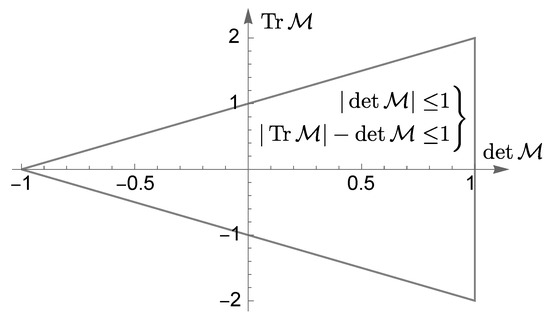
Figure 1.
The stability domain for matrix , which generates a discrete map on . If the point is inside the triangle, the eigenvalues of are inside the unit circle. It is the root condition, e.g., see [27]. The same applies to a mapping on generated by , where is a unitary matrix. In the area-preserving case (), the root condition reduces to .

Table 1.
Constraints on h that guarantee that both eigenvalues of are inside the unit circle. We consider additive splittings, the multiplicative Lie–Trotter splitting (2) is shown for reference. The second Strang splitting (9) cannot be used. The Burstein and Mirin splitting (10) is more restrictive than the Lie–Trotter splitting but gives better accuracy. The ARBBC splitting (11) is both more accurate and less restrictive.
In what follows, we will extend these results from a simple linear oscillator to a model equation that is relevant in fiber-optics. The problem breaks into a one-parametric set of two dimensional sub-problems and the root condition in Figure 1 applies to each sub-problem. An additional difficulty is that the system in question can experience “true” instabilities that are addressed by the continuous model equations. These instabilities should be properly recovered by a splitting scheme and separated from the unwanted numerical instabilities.
2. Model Equation
In the reminder of the manuscript, we use splitting methods to describe the evolution of nonlinear dispersive waves, which are important in many physical systems [28,29]. We assume that the waves are forced to propagate in one direction (along z axis) by the geometry of the system, like pulses in optical fibers. The wave field is given by the real part of the expression , where and are the carrier wave vector and angular carrier frequency, respectively. The complex envelope describes wave modulations. Except for extremely short pulses, evolves on a time scale much longer than , which is the slowly varying envelope approximation (SVEA).
If is constant and sufficiently small, the resulting wave is linear and monochromatic. It only exists if a certain dispersion relation is satisfied. In the vicinity of , the dispersion relation is typically approximated by a polynomial, e.g., of order like in [30]. Note that an envelope oscillation at the frequency is translated into a field oscillation at the frequency . The approximate dispersion law is written as
where is the group velocity at carrier frequency, is called the dispersion function. The dispersion coefficients formally refer to the derivatives at . In practice, they may be fitting parameters. The simplest nontrivial example of Equation (13) is for , the parameter describes the group velocity dispersion. In an ideal material with constant index of refraction, vanishes.
Equation (13) cannot hold for all possible , no matter how large the parameter J is [31]. In a numerical solution, however, we are always dealing with a limited bandwidth. Moreover, SVEA implies that for the main part of the spectrum, in which case all pulses propagate with velocities close to . It is convenient to set , where is the delay variable. The limited bandwidth refers to the Fourier transform of with respect to . In the following, denotes the transformed envelope, its bandwidth is given by
where is the step size on the -axis and is the angular Nyquist frequency. It is sufficient to require that Equation (13) holds on the interval (14). In practice, only a finite number of points, say , can be used on the axis. Therefore we impose a periodicity condition
where is also the number of harmonics after the discrete Fourier transform of the envelope. The harmonics are subject to the inequality (14) with the peculiarity that two limiting physical modes with correspond to one discrete mode. The period T must be much larger than the temporal width of all pulses.
The evolution equation for the complex envelope is derived using one or another form of multiscale expansion [32]. The result is the so-called generalized nonlinear Schrödinger equation (GNLSE) [33]
The parameter accumulates contributions by the cubic nonlinear interactions, which are assumed to be instantaneous. Equation (16) reduces to the nonlinear Schrödinger equation (NLSE) when .
The simplest nontrivial solution of Equation (16) reads
Equation (17) describes an unperturbed carrier wave with power proportional to . It is convenient to introduce the dimensionless parameter
which will appear later in the stability analysis of the solution (17) by the numerical schemes with the evolution step h.
GNLSE (16) is a bit special because it is solved along the space variable, while the time variable serves as the coordinate. Given at a fixed z and all , we want to calculate . For example, given the input pulse at one end of the fiber, we look for the outgoing pulse at the other end. This means, of course, that all waves propagate in the same direction and there are no reflected waves, which is a unidirectional approximation. The latter replaces SVEA in modern derivations of GNLSE-type models [34,35,36]. Such models get a more complex nonlinear term than in Equation (16) and are beyond the scope of this study.
2.1. GNLSE Splitting
An important feature of Equation (16) is that GNLSE is well suited for splitting methods. By separating linear and nonlinear terms in Equation (16), we see that the reduced equations (3) are easy to handle. The nonlinear one has a simple analytical solution
The linear one is solved by transforming to its frequency components
where
Calculation of the nonlinear and linear evolution operators is then limited by the rounding errors and by the properties of the discrete Fourier transform.
Equations (19) and (20) are formally exact. Nevertheless, solution of NLSE and GNLSE by splitting methods can suffer from numerical instabilities. The latter are typically weak, but can be observed at longer propagation distances, see [37]. With respect to NLSE, for example, the classical study [38] (see also [39,40,41]) established that the simplest first-order splitting (2) is stable if the evolution step h obeys the inequality
These results were generalized for GNLSE in [42,43]. An extension to the fourth-order Suzuki–Yoshida splitting (6) was reported in [44], and to an arbitrary multiplicative splitting in [45], again in the GNLSE framework. The extension for the additive splitting methods (9)–(11) will be reported below.
It should be noted that the numerical solution of GNLSE on a modern computer is fast. Even if the exact criterion (21) is unknown, it would not take long to perform a series of numerical experiments decreasing the solution step h until all numerical instabilities disappear. However, the brute force approach does not always work well. For example, finding a suitable dispersion profile or calculating the statistical properties of the optical field in fibers requires thousands GNLSE solutions [46,47]. This is time-consuming on any computer, and it would be advantageous to know in advance the generalization of the criterion (21) for the numerical method at hand. Another example is optical supercontinuum calculations [48]. The resulting spectrum is extremely wide and without a precise criterion it is difficult to distinguish between the physical modes and the numerical instability.
2.2. Modulation Instability
Following the pioneering work of Weideman and Herbst [38], the correctness of splitting methods is tested using modulation instability (MI), which is a fundamental phenomenon in the field of nonlinear waves [49]. MI occurs when small spontaneous modulations of the initially uniform carrier wave begin to grow, leading to the emergence of various localized structures, such as robust solitary pulses [50] or spontaneous rogue waves [51].
The initial stage of MI is described by considering a small perturbation of the solution (17)
Equation (16) is linearized with respect to , which gives
The entire solution space of Equation (22) can be divided into two-dimensional subspaces parameterized by the offset frequency . For this, use substitution
which gives a system of two coupled ODEs for each
It is convenient to split the dispersion function into odd and even components
The standard analysis shows that the equilibrium state of the system (24) is unstable if [52]
The inequality (26) gives offsets for which spontaneous growth of the perturbations (23) is expected. The offsets with the fastest growth are determined by , in which case grow as .
Analogous to from Equation (18), it is convenient to introduce a dimensionless phase parameter
where a “small” evolution step h is multiplied by a polynomial, which can take “large” values at the end of the frequency interval (14). This is a potential source of numerical instability. The main idea of the pioneer study [38] was that a correct splitting scheme should reproduce the true instability domain from Equation (26)
while no other instabilities should appear. This idea will be applied to additive splitting schemes in the following.
2.3. Split-Step Framework for Modulation Instability
To apply Equation (24) to the analysis of split-step methods, we must write its solution in the form (1). For this purpose, we introduce the matrix notations
such that Equation (24) takes the form
For the case at hand, Equation (1) reads
Note that the expressions for and , which were defined in advance in Equations (18) and (27), appear naturally in Equation (30). The stability properties of the discrete map (30) depend only on the matrix .
Furthermore, by separating contributions arising from linear and nonlinear terms in GNLSE (16), we see that, e.g., the simplest Lie–Trotter scheme (2) corresponds to the approximation
where and denote numerical approximations to and . This approximation is inexact because Equation (29) gives .
A generic multiplicative splitting (4) gives the approximation
and for, e.g., the second Strang splitting (9), we obtain
The remaining additive splittings (10) and (11) give similar, only more cumbersome formulas. These formulas will be used in the next section to investigate the applicability of the splitting methods.
3. Applications
We are in a good position to note that the standard MI analysis, normally performed with ODEs (24), can be performed with the matrix solution (30). To this end, one calculates
and applies the root condition from Figure 1. The instability in this case occurs when . The result agrees with the MI condition (28).
Similar analysis can be done with any multiplicative or additive splitting that approximates Equation (30). There may be several areas of instability. One should agree with Equation (28), the others should disappear as .
3.1. Lie–Trotter Splitting
It is instructive to revisit the Lie–Trotter approximation [38,39,42,43,44,45], which is described by Equation (31) with
The criterion from Figure 1 shows that the instability occurs when
Considering , the instability can be expected where . Expanding Equation (34) near , one gets the true MI domain (28). Expanding near , one gets the second domain with the numerical instability. The latter is avoided when is properly bounded, see Figure 2.
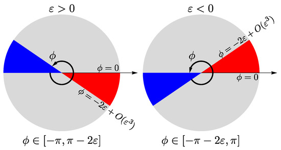
Figure 2.
Given , inequality (34) gives two instability domains for the angle parameter . The true MI domain (28) is red; the numerical instability domain is blue. To avoid the numerical instability, we impose restrictions on —they are shown at the bottom of the figure. For simplicity, the restrictions are combined in a single sufficient condition (35).
For the simplest focusing NLSE, where and , it is sufficient to require that . This results in Equation (21) from Ref. [38]. In general, the even part of the dispersion function in Equation (27) can change its sign and we can impose the constraint [43]
It should be satisfied for any offset within the total bandwidth (14). Equations (18) and (27) finally give
This is how the largest possible integration step h appears. In practice, one can simply require
and consider the result with tentativeness. We now have everything we need to generalize Equation (36) for the additive methods (9)–(11).
3.2. The Second Strang Splitting
The second Strang splitting (9) leads to Equation (33), so we should study the following evolution matrix
The root conditions from Figure 1 are violated because . Therefore, the second Strang splitting scheme cannot be used at all, as one would expect from the Table 1.
Consider, for example, a GNLSE with only
which applies to pulses in fibers with a specially managed dispersion law [53]. For what follows, it is convenient to normalize Equation (37). We indicate the dimensionless variables by dashes and define:
such that the amplitude is normalized using the base solution (17), the space using the so-called nonlinear length , and the delay is scaled such that . The normalized discrete frequencies are then integers . Recall that the number of harmonics and period T were introduced in Equation (15). Equation (18) indicates that the normalized step .
The normalized Equation (37) depends on a single parameter and on the sign of , we assume . The continuous wave solution (17) has the form . The MI condition (26) reduces to , i.e., the continuous wave should be stable for . Let us check this numerically.
Figure 3 shows solutions of Equation (37) obtained by two different splitting methods, where in both cases
and noise amplitude is . The Lie–Trotter method is stable, see Figure 3a,c. Here, Equation (36) requires , which is satisfied. For, e.g., , the Lie–Trotter solution is destroyed by a numerical instability. The second Strang method is numerically unstable in any case, see Figure 3b,d. This instability cannot be repaired by decreasing .
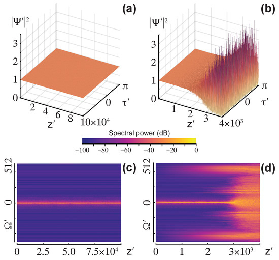
Figure 3.
Normalized power (3D plots) and spectral power (density plots). Equation (37) is solved for a slightly perturbed pump wave (17) using (a,c) Lie–Trotter and (b,d) additive Strang splittings with the same integration step h. The parameters from Equation (39) indicate that the pump is physically stable. This is confirmed by the Lie–Trotter solution because h is below the limiting value (36). The additive Strang splitting is numerically unstable. A reduction in h does not help here.
3.3. Burstein and Mirin Splitting
By analogy with Equations (9) and (33), the Burstein and Mirin splitting (10) is related to the evolution matrix
with
where, for brevity, we use the notation . The full analysis of the root conditions from Figure 1 is not useful here. Instead, we note that (for , which is always met in practice) the root conditions are satisfied when . This gives the sufficient condition
cf. Equation (36). Roughly speaking, the Burstein and Mirin method (10) requires a two times smaller integration step than the simplest multiplicative splitting.
Consider, for example, the standard optical NLSE [33]
which we normalize following Equation (38). The normalized NLSE depends on and on the sign of , we assume . The MI condition (26) reduces to , such that MI is expected for . Specifically, we consider the following parameters
noise amplitude is . Equation (40) gives , we then consider and .
Figure 4 uses , the solution (17) is then physically stable. This agrees with the numerical solution for in Figure 4a,c. For the wave is destroyed by the numerical instability, see Figure 4b,d.
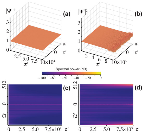
Figure 4.
Normalized power (3D plots) and spectral power (density plots). Equation (41) is solved for a slightly perturbed pump wave (17) using the Burstein-Mirin splitting for two different steps h. Parameters are from Equation (42). We choose such that the pump is physically stable. (a,c) h is slightly below the critical value from Equation (40) such that the stable pump is correctly reproduced by the numerical solution. (b,d) h is slightly above the critical value and the pump is destroyed by the numerical instability.
Figure 5 uses . The onset of MI is observed in Figure 5a,b, which was calculated for . This solution is destroyed by the numerical instability as z increases, see Figure 5c. The numerical instability is removed and MI is unaffected for .
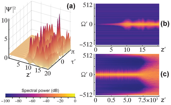
Figure 5.
Normalized power (3D plot) and spectral power (density plots). Equation (41) is solved for a slightly perturbed pump wave (17) using the Burstein-Mirin splitting for two different steps h. Parameters are from Equation (42). We choose such that the pump is physically unstable. (a,b) h is slightly below the critical value from Equation (40) and onset of MI is reproduced by the numerical solution. (c) h is slightly above the critical value and MI development is distorted the numerical instability.
3.4. ARBBC Splitting
By analogy with Equations (9) and (33), the ARBBC splitting (11) is related to the evolution matrix
with
where we recall that .
By expanding and in the vicinity of and applying the root conditions from Figure 1, we deduce that numerical stability is ensured when
cf., the conditions at the bottom of Figure 2. The sufficient criterion (35) is then replaced by
In practical terms, Equation (45) means that to a good approximation, Equation (36) also applies to the ARBBC splitting, which is also confirmed by numerical experiments.
Consider, for example, GNLSE of the form
with . If Equation (46) is carelessly reduced to the standard NLSE (41), the continuous wave solution (17) appears to be stable, but the stability is destroyed by a negative term, see [54,55,56,57]. This situation is called the four-wave mixing (FWM) instability [52].
Following Equation (38), the normalized Equation (46) depends on with . The MI condition (26) reduces to and here yields the FWM instability. Specifically, we consider the following parameters
noise amplitude is . Equation (45) requires . For the onset of the FWM instability should be correctly reproduced by the ARBBC splitting. For , however, the root conditions are additionally violated for , which indicates presence of the numerical instability. The latter develops extremely slowly and to make it visible we modified the initial condition by adding two small seed waves precisely at . The seed waves should remain bounded for and should slowly grow for . This is illustrated in Figure 6.
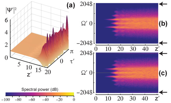
Figure 6.
Normalized power (3D plot) and spectral power (density plots). Equation (46) is solved for a slightly perturbed pump wave (17) using the ARBBC splitting for two different steps h. Parameters are from Equation (47), the pump is physically unstable due to the FWM instability. (a) h is slightly below the critical value from Equation (45) and onset of the FWM instability is reproduced by the numerical solution. (b) spectral picture, two seed perturbations indicated by arrows remain bounded. (c) h is slightly above the critical value, now the seed waves, which are intentionally imposed where the numerical instability is expected, slowly grow.
Figure 6a shows the normal onset of the FWM instability for . Figure 6b, gives the spectral picture, the seed waves are indicated by arrows and remain bounded. Figure 6c shows the spectral picture for , now the seed waves grow, although very slowly. The numerical instability, which is present where expected, is much less pronounced than in the previous calculations.
Last but not least, in the case of ARBBC splitting we face a new numerical instability. Indeed, expanding Equation (43) at , we get
The root conditions give the MI domain (28). However, a more accurate expansion of in Equation (43) yields
such that for . This indicates the existence of numerical instability, its domain overlaps the MI domain (28). Although such numerical instability is always present, its increment is extremely small. We were unable to identify a single instance in which the effect of this instability was observed. Although we cannot rigorously prove this, it appears that this numerical instability can be disregarded without any risk.
4. Conclusions
In conclusion, we have studied the restrictions on the numerical integration step h that provide a numerically stable split-step solution of the GNLSE (16). We used the technique originally developed for NLSE and for the simplest Lie–Trotter splitting [38] and subsequently extended to GNLSE and to various multiplicative splittings [39,42,43,44,45]. The technique has been applied here to three additive splittings (9)–(11), which are of interest because different threads of such splitting schemes can be computed independently on a multi-core machine.
The main idea is to study the fundamental problem of continuous wave stability directly for the splitting method in question and then to compare the output with the well-known results based on GNLSE. The fundamental fact is that both multiplicative and additive splitting schemes can lead to numerical instabilities, which tend to disappear with the decrease of h. This is how the limitation of the integration step appears.
The second Strang splitting [18] is numerically unstable for any h. The splitting reported by Burstein and Mirin [23] requires, roughly speaking, a two times smaller integration step than the multiplicative splittings. The additive splitting proposed in Ref. [24] can be used with the same integration step as the multiplicative splittings. With a small correction, the critical step is given by Equation (36). The latter criterion should be an integral part of any implementation of splitting solvers for GNLSE. This is especially important when the dispersion function in Equation (13) and, therefore, the differential operator in GNLSE are approximated by a higher-order polynomial.
A certain disadvantage of the approach proposed in [38] and used in this paper is that it employs only Equation (17), i.e., the simplest non-trivial solution of GNLSE (16). The resulting condition (36) is then necessary but not sufficient. In the numerical examples above the upper bound (36) is very close to the exact one, if not exact. See Appendix A for an example where this is not the case.
A natural question is what happens if we consider a more general seed solution? The problem should be considered first for NLSE (Equation (16) with ), which is integrable and has numerous analytic solutions [44]. In particular, solitary solutions are of interest because they are both extremely important in optics and observed in other systems that do not look like classical envelope equations, see e.g., [58]. Some work in this direction has been done for multiplicative splittings [39,40,41]. In the case of additive splittings, this challenge is waiting to be met. Furthermore, NLSE yields a hierarchy of integrable equations [44,59,60]. All of these models can potentially be studied using the above approach.
Author Contributions
Conceptualization, U.B. and R.Č.; methodology, S.A. and R.Č.; software, S.A.; validation, S.A., U.B. and R.Č.; investigation, S.A.; writing—original draft preparation, S.A.; writing—review and editing, U.B. and R.Č.; visualization, S.A.; supervision, U.B. All authors have read and agreed to the published version of the manuscript.
Funding
This research received no external funding.
Data Availability Statement
The original contributions presented in this study are included in the article material. Further inquiries can be directed to the corresponding author.
Conflicts of Interest
The authors declare no conflicts of interest.
Abbreviations
The following abbreviations are used in this manuscript:
| ARBBC | the additive splitting given by Equation (11) |
| FWM | four wave mixing |
| GNLSE | generalized nonlinear Schrödinger equation |
| MI | modulation instability |
| NLSE | nonlinear Schrödinger equation |
| SVEA | slowly varying envelope approximation |
Appendix A
The Appendix deals with the influence of terms with odd derivatives on numerical stability. Specifically, let us look at Equation (16) with
The above equation is the simplest way to account for the higher order dispersion effect and describes an important phenomenon of Cherenkov radiation [61]. In our context, it is important to note that the term in Equation (A1) has no effect on the MI condition (26). This is true for all odd dispersion coefficients, as it was found in the pioneering work on MI in GNLSE [62]. Similarly, odd dispersion coefficients do not affect the criterion (36), which for the present case is identical to the classical result (21) for NLSE [38].
On the other hand, the term in Equation (A1) has the highest derivative and should affect the numerical stability. To reveal this effect one needs a more general seed solution than Equation (17). The analysis is very complex even for the simplest multiplicative splitting, see [39,42,43]. Extending such an analysis to additive splittings is beyond the scope of this work. Here we are again confronted with the situation that Equation (36) only provides the upper bound for the integration step h. Let us demonstrate this numerically, this time using dimensional fiber parameters.
Equation (A1) was used to study the dispersion effect on MI in Section 8.2.7 of Ref. [63] with the coefficients
We consider a continuous pump wave with the power , fiber length is , relative noise amplitude is . The numerical solution is computed using harmonics over a time domain with the periodic boundary conditions.
Figure A1 shows the spectral density of the numerical solution of Equation (A1) by multiplicative Strang (a,b,c) and additive ARBBC (d,e,f) splittings. The solution is computed using decreasing integration steps (see panels from left to right), whereas Equation (21) yields . As we can see from the “wings” surrounding the main part of the spectrum, the numerical instability occurs much earlier than expected.
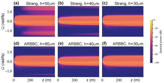
Figure A1.
Density plots of the spectral power for solutions of Equation (A1) with the parameters from Equation (A2). The solution step h decreases from left to right. The disappearing wings on the sides of the main spectrum show the disappearance of the numerical instability. However, the numerical instability is removed for smaller values of h than expected from Equation (21). The latter gives only upper estimate of the critical step (here ) in the case of the odd derivatives in GNLSE. Panels (a–c) show results from the standard multiplicative Strang splitting. Panels (d–f) show results from the additive ARBBC splitting, which performs considerably better.
References
- McLachlan, R.; Quispel, R. Splitting methods. Acta Numer. 2002, 11, 341–434. [Google Scholar] [CrossRef]
- Hundsdorfer, W.; Verwer, J. Numerical Solution of Time-Dependent Advection-Diffusion-Reaction Equations; Springer: Berlin/Heidelberg, Germany, 2003. [Google Scholar]
- Hairer, E.; Lubich, C.; Wanner, G. Geometric Numerical Integration. Structure-Preserving Algorithms for Ordinary Differential Equations, 2nd ed.; Springer Series in Computational Mathematics; Springer: Berlin/Heidelberg, Germany, 2006; Volume 31. [Google Scholar]
- Holden, H.; Karlsen, K.; Lie, K.A.; Risebro, H. Splitting Methods for Partial Differential Equations with Rough Solutions. Analysis and Matlab Programs; European Mathematical Society: Zürich, Switzerland, 2010. [Google Scholar]
- Glowinski, R.; Osher, S.J.; Yin, W. (Eds.) Splitting Methods in Communication, Imaging, Science, and Engineering; Scientific Computation; Springer: Berlin/Heidelberg, Germany, 2016. [Google Scholar]
- Buchholz, S.; Gauckler, L.; Grimm, V.; Hochbruck, M.; Jahnke, T. Closing the gap between trigonometric integrators and splitting methods for highly oscillatory differential equations. IMA J. Numer. Anal. 2018, 38, 57–74. [Google Scholar] [CrossRef]
- Musetti, S.; Serena, P.; Bononi, A. On the Accuracy of Split-Step Fourier Simulations for Wideband Nonlinear Optical Communications. J. Light. Technol. 2018, 36, 5669–5677. [Google Scholar] [CrossRef]
- de Negreiros Júnior, J.; do Nascimento e Sá Cavalcante, D.; de Moraes, J.; Marcelino, L.R.; de Carvalho Belchior Magalhães, F.; Barboza, R.R.; de Carvalho, M.; de Freitas Guimarães, G. Ultrashort pulses propagation through different approaches of the Split-Step Fourier method. J. Mechatronics Eng. 2018, 1, 2–11. [Google Scholar] [CrossRef]
- Zia, H. Simulation of white light generation and near light bullets using a novel numerical technique. Commun. Nonlinear Sci. Numer. Simul. 2018, 54, 356–376. [Google Scholar] [CrossRef]
- Rahman, A.; Dutta, N. Mid-Infrared Supercontinuum Generation in Highly Nonlinear Chalcogenide Fibers. Int. J. High Speed Electron. Syst. 2024, 33, 2440060. [Google Scholar] [CrossRef]
- Lakoba, T.I. Study of instability of the Fourier split-step method for the massive Gross–Neveu model. J. Comput. Phys. 2020, 402, 109100. [Google Scholar] [CrossRef]
- Xiang, L.; Jin, S.; Shao, W.; Gao, M. Evaluation of Crosstalk in Nonlinear Regime for Weakly Coupled Multi-Core Fiber With Random Perturbations Using a Split-Step Numerical Model. J. Light. Technol. 2023, 41, 5729–5736. [Google Scholar] [CrossRef]
- Cardoso, W.B. Alternative split-step method for solving linearly coupled nonlinear Schrödinger equations. Comput. Phys. Commun. 2025, 307, 109414. [Google Scholar] [CrossRef]
- Lu, W.; Yang, J.; Tian, X. Fourth-order split-step pseudo-spectral method for the modified nonlinear Schrödinger equation. Ships Offshore Struct. 2017, 12, 424–432. [Google Scholar] [CrossRef]
- Kormann, K.; Reuter, K.; Rampp, M. A massively parallel semi-Lagrangian solver for the six-dimensional Vlasov–Poisson equation. Int. J. High Perform. Comput. Appl. 2019, 33, 924–947. [Google Scholar]
- Zlotnik, A.; Ĉiegis, R. On Construction and Properties of Compact 4th Order Finite-Difference Schemes for the Variable Coefficient Wave Equation. J. Sci. Comput. 2023, 95, 3. [Google Scholar] [CrossRef]
- Zhu, X.; Wan, H.; Zhang, Y. A split-step finite element method for the space-fractional Schrödinger equation in two dimensions. Sci. Rep. 2024, 14, 24257. [Google Scholar] [CrossRef]
- Strang, G. Accurate Partial Difference Methods I: Linear Cauchy Problems. Arch. Rat. Mech. Anal. 1963, 12, 392–402. [Google Scholar] [CrossRef]
- Strang, G. On the Construction and Comparison of Difference Schemes. SIAM J. Numer. Anal. 1968, 5, 506–517. [Google Scholar] [CrossRef]
- Suzuki, M. Fractal decomposition of exponential operators with applications to many-body theories and Monte Carlo simulations. Phys. Lett. A 1990, 146, 319–323. [Google Scholar] [CrossRef]
- Yoshida, H. Construction of higher order symplectic integrators. Phys. Lett. A 1990, 150, 262–268. [Google Scholar] [CrossRef]
- Blanes, S.; Moan, P.C. Practical symplectic partitioned Runge-Kutta and Runge-Kutta-Nyström methods. J. Comput. Appl. Math. 2002, 142, 313–330. [Google Scholar] [CrossRef]
- Burstein, S.Z.; Mirin, A.A. Third order difference methods for hyperbolic equations. J. Comput. Phys. 1970, 5, 547–571. [Google Scholar] [CrossRef]
- Amiranashvili, S.; Radziunas, M.; Bandelow, U.; Busch, K.; Čiegis, R. Additive splitting methods for parallel solutions of evolution problems. J. Comput. Phys. 2021, 436, 110320. [Google Scholar] [CrossRef]
- Taha, T.; Ablowitz, M. Analytical and numerical aspects of certain nonlinear evolution equations. II. Numerical, nonlinear Schrödinger equation. J. Comput. Phys. 1984, 55, 231–253. [Google Scholar] [CrossRef]
- Lovisetto, M.; Clamond, D.; Marcos, B. Integrating factor techniques applied to the Schrödinger-like equations. Comparison with Split-Step methods. Appl. Numer. Math. 2024, 197, 258–271. [Google Scholar] [CrossRef]
- Štikonas, A. The root condition for polynomial of the second order and a spectral stability of finite-difference schemes for Kuramoto-Tsuzuki equation. Math. Model. Anal. 1998, 3, 214–226. [Google Scholar] [CrossRef]
- Whitham, G.B. Linear and Nonlinear Waves; John Wiley & Sons: New York, NY, USA, 1974. [Google Scholar]
- Boyd, R.W. Nonlinear Optics, 3rd ed.; Academic: New York, NY, USA, 2008. [Google Scholar]
- Dudley, J.M.; Genty, G.; Coen, S. Supercontinuum generation in photonic crystal fiber. Rev. Mod. Phys. 2006, 78, 1135–1184. [Google Scholar] [CrossRef]
- Oughstun, K.E.; Xiao, H. Failure of the Quasimonochromatic Approximation for Ultrashort Pulse Propagation in a Dispersive, Attenuative Medium. Phys. Rev. Lett. 1997, 78, 642–645. [Google Scholar] [CrossRef]
- Nayfeh, A.H. Perturbation Methods; Wiley: Hoboken, NJ, USA, 1973. [Google Scholar]
- Agrawal, G.P. Nonlinear Fiber Optics, 4th ed.; Academic: New York, NY, USA, 2007. [Google Scholar]
- Brabec, T.; Krausz, F. Nonlinear Optical Pulse Propagation in the Single-Cycle Regime. Phys. Rev. Lett. 1997, 78, 3282–3285. [Google Scholar] [CrossRef]
- Kinsler, P. Optical pulse propagation with minimal approximations. Phys. Rev. A 2010, 81, 013819. [Google Scholar] [CrossRef]
- Kolesik, M.; Jakobsen, P.; Moloney, J.V. Quantifying the limits of unidirectional ultrashort optical pulse propagation. Phys. Rev. A 2012, 86, 035801. [Google Scholar] [CrossRef]
- Lakoba, T.I. Long-Time Simulations of Nonlinear Schrödinger-Type Equations using Step Size Exceeding Threshold of Numerical Instability. J. Sci. Comput. 2017, 72, 14–48. [Google Scholar] [CrossRef]
- Weideman, J.A.C.; Herbst, B.M. Split-Step Methods for the Solution of the Nonlinear Schrödinger Equation. SIAM J. Numer. Anal. 1986, 23, 485–507. [Google Scholar] [CrossRef]
- Lakoba, T.I. Instability analysis of the split-step Fourier method on the background of a soliton of the nonlinear Schrödinger equation. Numer. Methods Partial. Differ. Equations 2012, 28, 641–669. [Google Scholar] [CrossRef]
- Lakoba, T.I. Instability of the finite-difference split-step method applied to the nonlinear Schrödinger equation. I. standing soliton. Numer. Methods Partial. Differ. Equ. 2016, 32, 1002–1023. [Google Scholar] [CrossRef]
- Lakoba, T.I. Instability of the finite-difference split-step method applied to the nonlinear Schrödinger equation. II. moving soliton. Numer. Methods Partial. Differ. Equ. 2016, 32, 1024–1040. [Google Scholar] [CrossRef]
- Lakoba, T.I. Instability of the split-step method for a signal with nonzero central frequency. J. Opt. Soc. Am. B 2013, 30, 3260–3271. [Google Scholar] [CrossRef]
- Severing, F.; Bandelow, U.; Amiranashvili, S. Spurious Four-Wave Mixing Processes in Generalized Nonlinear Schrödinger Equations. J. Light. Technol. 2023, 41, 5359–5365. [Google Scholar] [CrossRef]
- Yang, J. Nonlinear Waves in Integrable and Nonintegrable Systems; SIAM: Philadelphia, PA, USA, 2010. [Google Scholar]
- Amiranashvili, S.; Čiegis, R. Stability of the higher-order splitting methods for the nonlinear Schrödinger equation with an arbitrary dispersion operator. Math. Model. Anal. 2024, 29, 560–574. [Google Scholar] [CrossRef]
- Kraych, A.E.; Agafontsev, D.; Randoux, S.; Suret, P. Statistical Properties of the Nonlinear Stage of Modulation Instability in Fiber Optics. Phys. Rev. Lett. 2019, 123, 093902. [Google Scholar] [CrossRef]
- Dudley, J.M.; Genty, G.; Mussot, A.; Chabchoub, A.; Dias, F. Rogue waves and analogies in optics and oceanography. Nat. Rev. Phys. 2019, 1, 675–689. [Google Scholar] [CrossRef]
- Sylvestre, T.; Genier, E.; Ghosh, A.N.; Bowen, P.; Genty, G.; Troles, J.; Mussot, A.; Peacock, A.C.; Klimczak, M.; Heidt, A.M.; et al. Recent advances in supercontinuum generation in specialty optical fibers. J. Opt. Soc. Am. B 2021, 38, F90–F103. [Google Scholar] [CrossRef]
- Zakharov, V.E.; Ostrovsky, L.A. Modulation instability: The beginning. Phys. D Nonlinear Phenom. 2009, 238, 540–548. [Google Scholar] [CrossRef]
- Hasegawa, A.; Matsumoto, M. Optical Solitons in Fibers; Springer: Berlin/Heidelberg, Germany, 2003. [Google Scholar]
- Erkintalo, M.; Hammani, K.; Kibler, B.; Finot, C.; Akhmediev, N.; Dudley, J.M.; Genty, G. Higher-Order Modulation Instability in Nonlinear Fiber Optics. Phys. Rev. Lett. 2011, 107, 253901. [Google Scholar] [CrossRef] [PubMed]
- Yu, M.; McKinstrie, C.J.; Agrawal, G.P. Modulational instabilities in dispersion-flattened fibers. Phys. Rev. E 1995, 52, 1072–1080. [Google Scholar] [CrossRef] [PubMed]
- Blanco-Redondo, A.; de Sterke, C.M.; Sipe, J.E.; Krauss, T.F.; Eggleton, B.J.; Husko, C. Pure-quartic solitons. Nat. Commun. 2016, 7, 10427. [Google Scholar] [CrossRef]
- Kitayama, K.; Okamoto, K.; Yoshinaga, H. Extended four-photon mixing approach to modulational instability. J. Appl. Phys. 1988, 64, 6586–6587. [Google Scholar] [CrossRef]
- Cavalcanti, S.B.; Cressoni, J.C.; da Cruz, H.R.; Gouveia-Neto, A.S. Modulation instability in the region of minimum group-velocity dispersion of single-mode optical fibers via an extended nonlinear Schrödinger equation. Phys. Rev. A 1991, 43, 6162–6165. [Google Scholar] [CrossRef]
- Pitois, S.; Millot, G. Experimental observation of a new modulational instability spectral window induced by fourth-order dispersion in a normally dispersive single-mode optical fiber. Opt. Commun. 2003, 226, 415–422. [Google Scholar] [CrossRef]
- Harvey, J.D.; Leonhardt, R.; Coen, S.; Wong, G.K.L.; Knight, J.C.; Wadsworth, W.J.; Russell, P.S.J. Scalar modulation instability in the normal dispersion regime by use of a photonic crystal fiber. Opt. Lett. 2003, 28, 2225–2227. [Google Scholar] [CrossRef]
- Chua, C.; Liu, H. Existence of positive solutions for a quasilinear Schrödinger equation. Nonlinear Anal. Real World Appl. 2018, 44, 118–127. [Google Scholar] [CrossRef]
- Ankiewicz, A.; Kedziora, D.J.; Chowdury, A.; Bandelow, U.; Akhmediev, N. Infinite hierarchy of nonlinear Schrödinger equations and their solutions. Phys. Rev. E 2016, 93, 012206. [Google Scholar] [CrossRef]
- Bandelow, U.; Ankiewicz, A.; Amiranashvili, S.; Akhmediev, N. Sasa-Satsuma hierarchy of integrable evolution equations. Chaos 2018, 28, 053108. [Google Scholar] [CrossRef]
- Akhmediev, N.; Karlsson, M. Cherenkov radiation emitted by solitons in optical fibers. Phys. Rev. A 1995, 51, 2602–2607. [Google Scholar] [CrossRef] [PubMed]
- Potasek, M.J. Modulation instability in an extended nonlinear Schrödinger equation. Opt. Lett. 1987, 12, 921–923. [Google Scholar] [CrossRef] [PubMed]
- Dudley, J.M.; Taylor, J.R. (Eds.) Supercontinuum Generation in Optical Fibers; Cambridge University Press: Cambridge, UK, 2010. [Google Scholar]
Disclaimer/Publisher’s Note: The statements, opinions and data contained in all publications are solely those of the individual author(s) and contributor(s) and not of MDPI and/or the editor(s). MDPI and/or the editor(s) disclaim responsibility for any injury to people or property resulting from any ideas, methods, instructions or products referred to in the content. |
© 2025 by the authors. Licensee MDPI, Basel, Switzerland. This article is an open access article distributed under the terms and conditions of the Creative Commons Attribution (CC BY) license (https://creativecommons.org/licenses/by/4.0/).