Dynamical Analysis of an Economic-Environment Model with Unilateral and Bilateral Control

Abstract

Air pollution is one of the most important environmental problems in the world, it does harm to human health as well as hindering the sustainable development of the economy. The grim situation deserves wide attention and active participation in improvement. Thus, in this paper, considering the pollution control and sustainable development of the economy, we develop and investigate the economic-environment model with unilateral and bilateral control. To begin with, we briefly describe the dynamic behavior of the free system. It then follows the analysis of the system with unilateral and bilateral control. The existence of the order-1 and order-2 periodic solutions are investigated under different conditions. In addition, their stability is proven. The results show that the bilateral control strategy is beneficial to the sustainable development of economy.

1. Introduction

The excessive consumption of fossil fuels over the past few decades has produced substantial carbon dioxide (CO₂) emissions, resulting in a series of severe environmental issues (e.g., global warming, rising sea levels, etc) [1]. These problems have threatened the sustainable development of humanity [2]. Notably, the World Meteorological Organization (WMO) reported that the 2023 global average temperature reached 1.45 °C above pre-industrial levels, underscoring the existential urgency of reconciling economic growth with ecological preservation. This tension is epitomized by China, whose rapid industrialization transformed it into the world’s second-largest economy-yet at a staggering environmental cost [3,4].

As the largest CO₂ emitter, China accounted for approximately 28.8% of global carbon dioxide emissions in 2022 (IEA), with a carbon emission intensity per unit GDP 2–3 times higher than that of developed nations. Concurrently, air pollution has become a public health emergency: the national average PM_2.5 concentration exceeds the WHO Global Air Quality Guideline by fivefold [5], linked to 1.34 million premature deaths in 2021 alone [6]. Alarmingly, health risks persist even at PM_2.5 levels below 10 μg/m³ [7], highlighting the inadequacy of current mitigation efforts. In response, China’s dual-carbon goals—peaking emissions by 2030 and achieving carbon neutrality by 2060 [8]—represent both a national commitment and a microcosm of the global sustainability dilemma.

This context raises critical questions: How do economic growth and environmental protection interact dynamically? What policy tools can equitably balance these competing priorities across regions and sectors? Answering these questions is imperative for designing actionable pathways toward sustainable development [9].

Therefore, an increasing number of scholars began to investigate the interaction of the economy and environmental pollution. Early works on economics and the environment pollution can be traced back to the 1970s [10,11]. In addition, the pollution is considered as a by-product of production, and the impact of pollution on economy was studied through the damage function [12,13,14,15]. The damage function drives the economy towards collapse only if the pollution takes infinite values, this means that there is no poverty trap caused by pollution, no matter how severe it is, and no matter what the initial conditions of the economic-environmental integrated system, which is barely acceptable. In order to avoid this phenomenon, the damage function must take into account the non-infinite elasticity of the environment, then Skiba pointed out an S-Shaped aggregate production function [16]. After that, the economic-environment model with S-Shaped production function has attracted the attention of scholars, and the corresponding dynamical behaviors are investigated. For example, Liuzzi and Venturi [17] proposed a minimal integrated economic-environment model as follows:

$$\left\{\begin{array}{c}{\displaystyle \frac{\mathrm{d}x\left(t\right)}{\mathrm{d}t}}={\displaystyle \frac{s(1-u)\alpha x^2\left(t\right)}{(1+by\left(t\right))(1+\alpha x^2\left(t\right))}}-{\delta }_{1}x\left(t\right),\hfill \\ {\displaystyle \frac{\mathrm{d}y\left(t\right)}{\mathrm{d}t}}={\displaystyle \frac{\theta (1-u)\alpha x^2\left(t\right)}{1+\alpha x^2\left(t\right)}}-{\delta }_{2}y\left(t\right),\hfill \\ x\left(0\right)=x_0,y\left(0\right)=y_0,\hfill \end{array}\right.$$

(1)

where $x\left(t\right)$ and $y\left(t\right)$ represent respectively the evolutions of capital and pollution, and $(x\left(0\right),y\left(0\right))=(x_0,y_0)$ is the initial value. ${\displaystyle \frac{\alpha x^2\left(t\right)}{1+\alpha x^2\left(t\right)}}$ is the production function, and ${\displaystyle \frac{1}{1+by\left(t\right)}}$ is the damage function. s is the saving ratio of the economy; $u\in (0,1)$ stands for the share of reduction in the abatement activities, thus $1-u$ represents the unabated emissions, ${\delta }_1$ is the depreciation rate of capital. $\theta$ is the degree of environmental inefficiency of economic activities, ${\delta }_2\in (0,1)$ is the self-cleaning of the environment. The authors studied the existence and stability of the equilibrium points, as well as the existence of bifurcations, such as the Hopf bifurcation and the Bogdanov–Takens bifurcation.

Now, industrial emissions have become a prominent source of air pollution, so it is increasingly necessary to control industrial emissions. The question then arose: ”what strategies should be taken to change this situation and maintain the sustainable development of economy?” The literature [18] showed that the most effective way to improve the natural environment is to reduce the intensity of major pollutant emissions. In addition to the O₃ and PM_2.5, there is a growing public concern about the health risks of the emerging organic compounds and heavy metals, which need to be addressed synergistically [19,20]. Compared with the evolution of pollution, the intensity of pollutant can be decreased in a short time with human intervention, this phenomenon can be thought of as an instantaneous action, and it could be described well by the impulsive differential equation which has been widely applied in many applications, such as integrated pest management [21,22], pharmacokinetics [23], conservation and utilization and conservation of resources [24,25,26], and commodity price regulation [27], etc.

Motivated by the aforementioned, in this paper, we present a mathematical model for the management of pollution and economy, and attempt to enrich the nonlinear research in the field of sustainable development form the point of view of mathematical modeling. On the one hand, economic development increases individual purchasing power and improves individual quality of life. On the other hand, while the economy has been growing rapidly, there are also problems with inefficient growth and excessive resource and environmental costs. Thus, the primary objective of this paper is to demonstrate that the principles of sustainable development should be adopted to balance these dual imperatives.

The rest of the paper is organized as follows: In Section 2, we present the economic-environment model with unilateral and bilateral control. In Section 3, we study the existence and stability of order-1 periodic solutions and order-2 periodic solutions of unilateral system model and bilateral system, respectively. In Section 4, we perform some numerical simulations to verify the validity of the theoretical results. The conclusion is presented in Section 5.

2. Model Formulation

As the application of semi-continuous dynamic system in the air pollution control, we mainly investigate the dynamical behaviors of an economic-environment model with bilateral control. On the one hand, when the economy is at a lower level, the priority should be given to the economic development. So we are committed to developing economy to make the quantity of capital not less than $h_1$. On the other hand, high pollution will limit economic development and may lead to economic collapse. Thus, in order to avoid economic collapse caused by high pollution, the density of pollution should be kept in a reasonable range $[0, h_2]$. Thus, we introduce the two control thresholds $x=h_1$ and $y=h_2$ into system (1). When the quantity of the capital decreases to $h_1$, by developing the economy, the quantity of the capital can be increased by a certain proportion, while the pollution will increase by a certain amount because the environmental pollution is regraded as a by-product of production [17]. When the density of pollution reaches to $h_2$, it is necessary to take measures to reduce pollution. For example, the Chinese government attached great importance to environmental pollution control and has continuously increased its input in this aspect [28,29,30,31]. The pollution control investment could decrease the amount of capital, and compared with the evolution of capital, this can be considered as a short time or instantaneous action. Thus, an economic-environment model with bilateral control is established as follows:

$$\left\{\begin{array}{c}\left.\begin{array}{c}{\displaystyle \frac{\mathrm{d}x}{\mathrm{d}t}}={\displaystyle \frac{s(1-u)\alpha x^2\left(t\right)}{(1+by\left(t\right))(1+\alpha x^2\left(t\right))}}-{\delta }_{1}x\left(t\right)\hfill \\ {\displaystyle \frac{\mathrm{d}y}{\mathrm{d}t}}={\displaystyle \frac{\theta (1-u)\alpha x^2\left(t\right)}{1+\alpha x^2\left(t\right)}}-{\delta }_{2}y\left(t\right)\hfill \end{array}\right\}x>h_1,y<h_2,\hfill \\ \left.\begin{array}{c}\Delta x=q_{1}x\hfill \\ \Delta y={\tau }_1\hfill \end{array}\right\}x=h_1,\hfill \\ \left.\begin{array}{c}\Delta x=-{\tau }_2\hfill \\ \Delta y=-q_{2}y\hfill \end{array}\right\}y=h_2,\hfill \\ x\left(0\right)>h_1,y\left(0\right)<h_2,0<q_1,q_2<1.\hfill \end{array}\right.$$

(2)

For system (2), combing the geometric theory of differential equations, we find that when it is dominated by only one of the two impulsive functions (see Definition A1 in Appendix A), then system (2) can become two unilateral control systems which are list as follows:

$$\left\{\begin{array}{c}\left.\begin{array}{c}{\displaystyle \frac{\mathrm{d}x}{\mathrm{d}t}}={\displaystyle \frac{s(1-u)\alpha x^2\left(t\right)}{(1+by\left(t\right))(1+\alpha x^2\left(t\right))}}-{\delta }_{1}x\left(t\right)\hfill \\ {\displaystyle \frac{\mathrm{d}y}{\mathrm{d}t}}={\displaystyle \frac{\theta (1-u)\alpha x^2\left(t\right)}{1+\alpha x^2\left(t\right)}}-{\delta }_{2}y\left(t\right)\hfill \end{array}\right\}y<h_2,\hfill \\ \left.\begin{array}{c}\Delta x=-{\tau }_2\hfill \\ \Delta y=-q_{2}y\hfill \end{array}\right\}y=h_2,\hfill \\ y\left(0\right)<h_2,0<q_2<1,\hfill \end{array}\right.$$

(3)

and

$$\left\{\begin{array}{c}\left.\begin{array}{c}{\displaystyle \frac{\mathrm{d}x}{\mathrm{d}t}}={\displaystyle \frac{s(1-u)\alpha x^2\left(t\right)}{(1+by\left(t\right))(1+\alpha x^2\left(t\right))}}-{\delta }_{1}x\left(t\right)\hfill \\ {\displaystyle \frac{\mathrm{d}y}{\mathrm{d}t}}={\displaystyle \frac{\theta (1-u)\alpha x^2\left(t\right)}{1+\alpha x^2\left(t\right)}}-{\delta }_{2}y\left(t\right)\hfill \end{array}\right\}x>h_1,\hfill \\ \left.\begin{array}{c}\Delta x=q_{1}x\hfill \\ \Delta y={\tau }_1\hfill \end{array}\right\}x=h_1,\hfill \\ x\left(0\right)>h_1,0<q_1<1.\hfill \end{array}\right.$$

(4)

In the following, we mainly investigate the dynamics of the three systems.

3. Main Results

In the following, the dynamics of system (1) are briefly introduced and the existence and stability of periodic solutions (see Definition A2 in Appendix A) of systems (2)–(4) are proved.

3.1. Dynamics of System (1)

For system (1), it always has a stable boundary equilibrium point $E_0(0,0)$. There exist two isoclines

$$l_1:\left\{(x,y)|{\displaystyle \frac{s(1-u)\alpha x\left(t\right)}{(1+by\left(t\right))(1+\alpha x^2\left(t\right))}}-{\delta }_1=0\right\},$$

and

$$l_2:\left\{(x,y)|{\displaystyle \frac{\theta (1-u)\alpha x^2\left(t\right)}{1+\alpha x^2\left(t\right)}}-{\delta }_{2}y\left(t\right)=0\right\},$$

from which we have

$$y*={\displaystyle \frac{\theta (1-u)\alpha {x*}^2\left(t\right)}{{\delta }_2(1+\alpha {x*}^2\left(t\right))}},$$

and $x*$ is given by:

$${\delta }_1\alpha ({\delta }_2+b\theta (1-u))x^2-s{\delta }_2(1-u)\alpha x+{\delta }_1{\delta }_2\alpha =0.$$

Obviously, the curve $l_1$ has a horizontal asymptote $y={\displaystyle \frac{\theta (1-u)}{{\delta }_1}}$, and the curve $l_2$ has a horizontal asymptote $y=-{\displaystyle \frac{1}{b}}$.

Define $\Delta ={\left(s{\delta }_2(1-u)\alpha \right)}^2-4{\delta }_1^2{\alpha }^2{\delta }_2({\delta }_2+b\theta (1-u))$. If $\Delta =0$, then system (1) has one positive equilibrium point; if $\Delta <0$, then system (1) has no positive equilibrium point. If $\Delta >0$, then system (1) has two positive equilibrium points ($E_1^{*}(x_1^{*},y_1^{*})$ and $E_2^{*}(x_2^{*},y_2^{*})$), as is shown in Figure 1. $E_1^{*}$ is always a saddle point; the dynamics around $E_2^{*}$ are very complex, it can be referred to the reference [17]. In this paper, we mainly investigate the existence and stability of the periodic solutions for the case of that $E_2^{*}$ is a stable focus point. The other cases are similar to this one, so it is omitted.

3.2. Existence and Stability of the Periodic Solution

In this subsection, the existence and stability of periodic solutions for the case of that $E_2^{*}$ is a stable focus point are proved. Assume that $l_3$ and $l_4$ are two stable manifolds of system (1), as is shown in Figure 2. In the following text, they have the same meanings.

Now we discuss the existence of order-1 periodic solution for the case of $(1-q_2)h_2<h_2<y_2^{*}$, then we have the following Theorem 1.

Theorem 1. 

If $x_{B_1}>x_2^{*}>x_{A_1}$ and $x_{B_2}<x_{A_2}$, then system (3) exists an order-1 periodic solution.

Proof. 

Assume that $A_1$ is the intersection point of the curve $l_1$ and phase set $N_1$, then the trajectory from point $A_1$ intersects impulsive set $M_1$ at point $B_1$, and it is mapped to the point $A_1^{+}\in N_1$ which is the successor point of $A_1$ (see Definition A4 in Appendix A), according to the magnitude of $A_1^{+}$ and $A_1$, there are three cases.

(1)

If point $A_1^{+}$ overlaps point $A_1$, then $\widehat{A_1{B}_1{A}_1}$ forms an order-1 periodic solution.

(2)

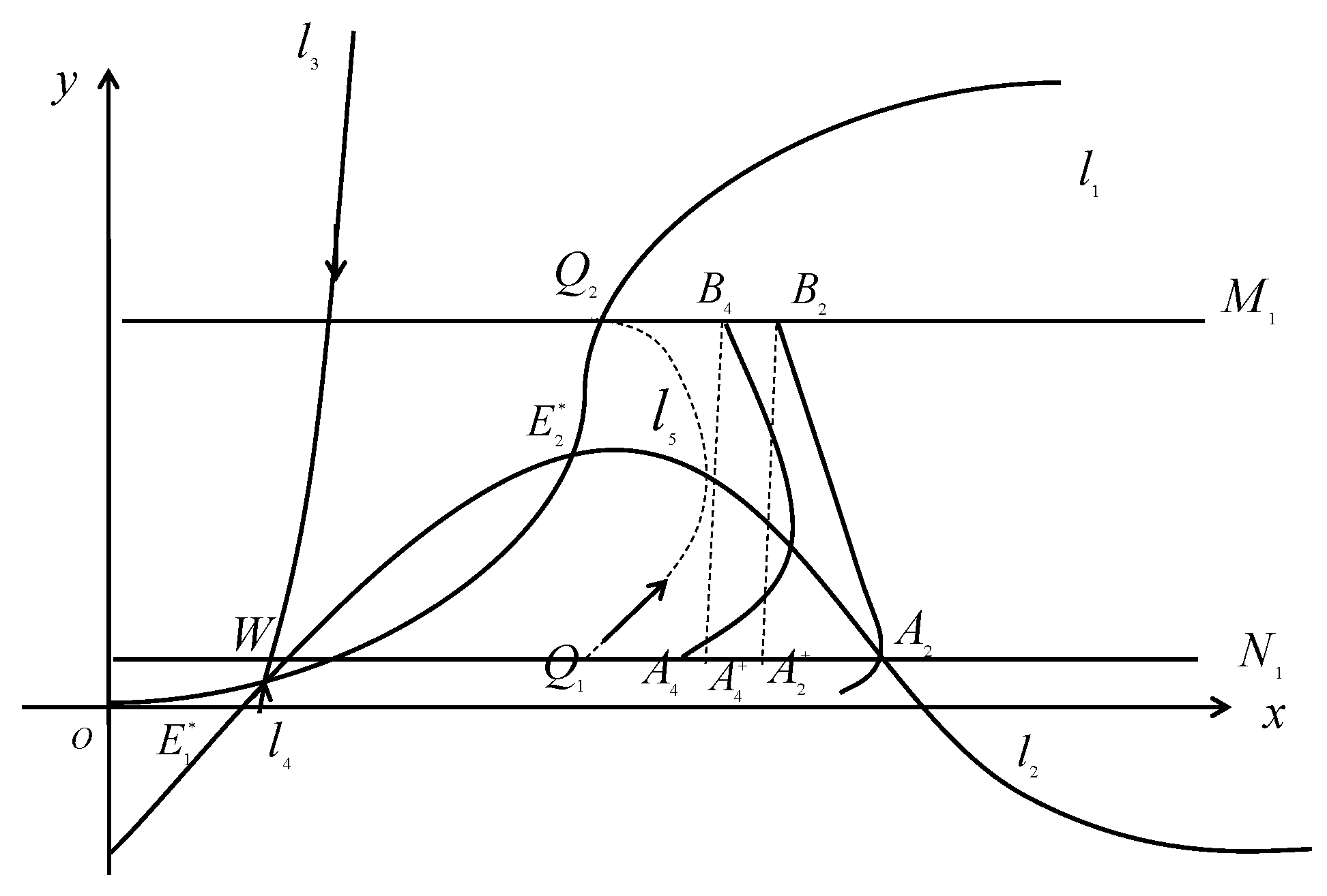
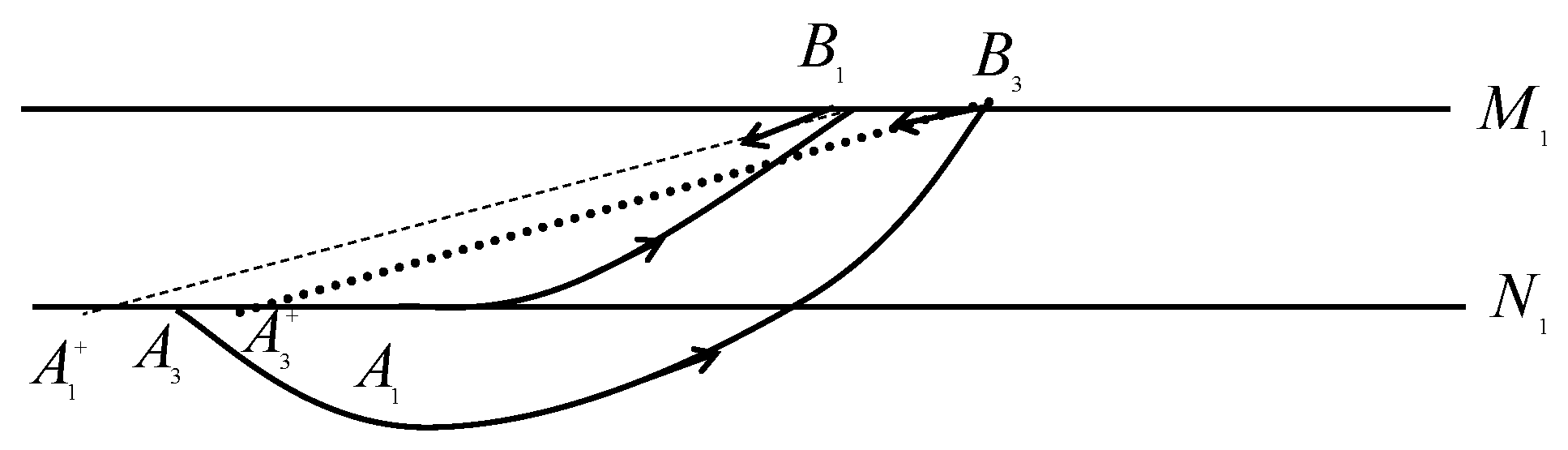
If point $A_1^{+}$ is located on the right side of $A_1$, this means that $x_{A_1^{+}}>x_{A_1}$, then the successor function $f\left(A_1\right)=x_{A_1^{+}}-x_{A_1}>0$. Now it is necessary to find a point such that the corresponding successor function is less than 0.

We can further assume that $A_2$ is the intersection point of the curve $l_2$ and phase set $N_1$, then there exists a trajectory passing through the point $A_2$, and it intersects the impulsive set at point $B_2$, then it jumps to the point $A_2^{+}\in N_1$ which is the successor point of $A_2$. It is easy to find that the successor function $f\left(A_2\right)=x_{A_2^{+}}-x_{A_2}<0$. Then, there is a point $S\in \overline{A_1{A}_2}$ such that $f\left(S\right)=0$, the existence of order-1 periodic solution is proved (see Figure 2a).

(3)

Let W be the intersection of $l_3$ and phase set $N_1$. If point $A_1^{+}$ is located on the left side of $A_1$, this means that $x_{A_1^{+}}<x_{A_1}$, then the successor function $f\left(A_1\right)=x_{A_1^{+}}-x_{A_1}<0$. In addition, we need to assume that $x_{A_1^{+}}>x_W$ (see Figure 2b). If not, the trajectory will tend to be the origin point.

In the following, it is necessary to find a point such that the corresponding successor function is more than 0. We choose a point $A_3$ is located on the right side of $A_1^{+}$, and it is very close to the point $A_1^{+}$, i.e., $x_{A_3}=x_{A_1^{+}}+\epsilon$ where $\epsilon$ is extremely small (In the following text, $\epsilon$ still represents a very small number). Trajectory form point $A_3$ intersects impulsive set $M_1$ at point $B_3$, then it is mapped into phase set $N_1$ at point $A_3^{+}$. Here, we have $x_{A_3^{+}}=x_{B_3}-{\tau }_2$, $x_{A_1^{+}}=x_{B_1}-{\tau }_2$, then $f\left(A_3\right)=x_{B_3}-x_{B_1}-\epsilon >0$ due to $x_{B_3}>x_{B_1}$. Then there exists a point $S\in \overline{A_1{A}_3}$ such that $f\left(S\right)=0$, then the existence of order-1 periodic solution for system (3) is proved (see Figure 3), and Figure 3 is partial enlargement of Figure 2b. □

In the following, we discuss the existence of order-1 periodic solution for the case of $(1-q_2)h_2<x_2^{*}<h_2$.

Theorem 2. 

If $x_{Q_1}<x_{A_3}<x_{B_3}$ and $x_{B_2}<x_{A_2}$, then system (3) exists an order-1 periodic solution.

Proof. 

Let $Q_2$ be the intersection of the curve $l_1$ and the impulsive set $M_1$, then there exists a trajectory $l_5$ from the point $Q_1\in N_1$ which is tangent to the impulsive set at point $Q_2$. Taking a point $A_4(x_{A_4},y_{A_4})\in N_1$, where $x_{A_4}=x_{Q_1}+\epsilon$. Here, we still assume that the trajectory from point $A_2$ must intersect $M_1$ at point $B_2$, then it is mapped to $A_2^{+}(x_{A_2^{+}},y_{A_2^{+}})\in N_1$, the magnitude of $x_{A_4}$ and $x_{A_4^{+}}$ can be divided into three cases.

(1)

If $x_{A_4}=x_{A_4^{+}}$, then $\widehat{A_4{B}_4{A}_4}$ forms an order-1 periodic solution.

(2)

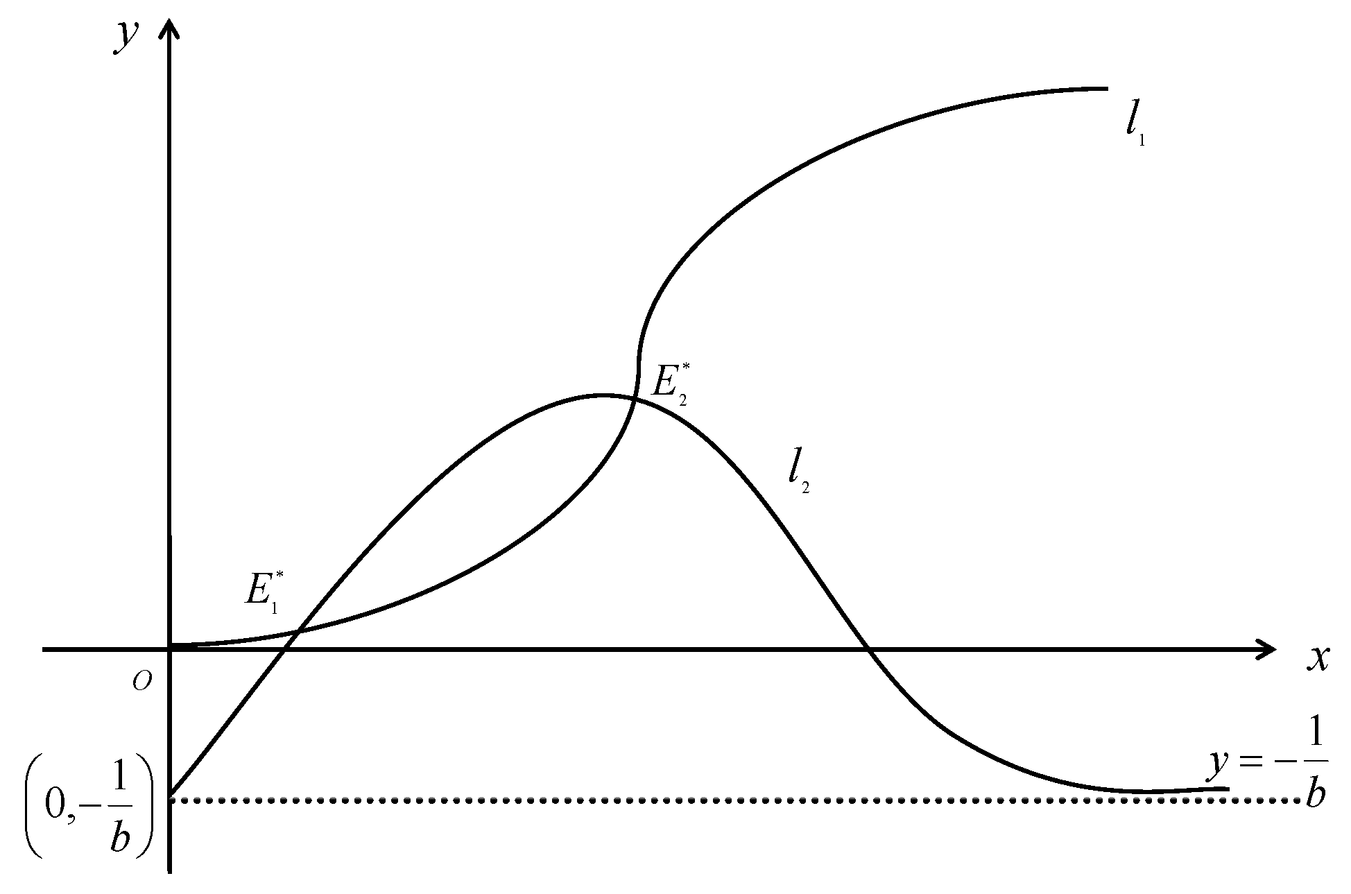
If $x_{A_4}>x_{A_4^{+}}>x_W$, then the trajectory will tend to $E_2^{*}$, system (3) does not exist periodic solution. If $x_{A_4^{+}}<x_W$, i.e., $x_{B_4}-{\tau }_2<x_W$, then it will tend to the origin point.

(3)

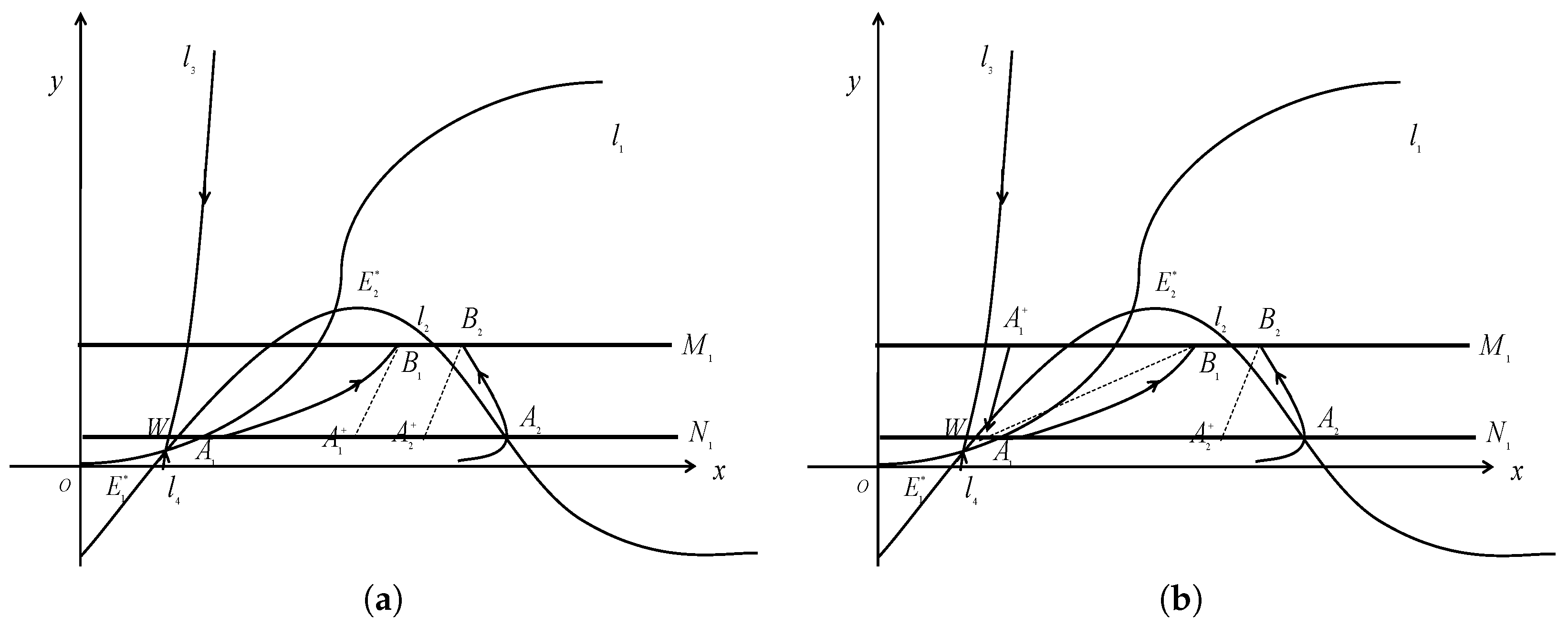
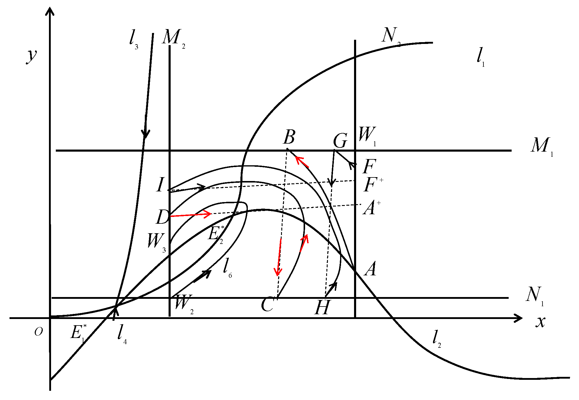
If $x_{A_4}<x_{A_4^{+}}$, then the successor function $f\left(A_4\right)=x_{A_4^{+}}-x_{A_4}>0$. Now it is necessary to choose a point such that the corresponding successor function is less than 0. We further assume that $A_2$ is the intersection point of the curve $l_2$ and phase set $N_1$, then there exists a trajectory passing through the point $A_2$, by the geometric theory of differential equation, it will intersect the impulsive set at point $B_2$, then it is mapped to the point $A_2^{+}\in N_1$, where $A_2^{+}$ is the successor point of $A_2$. Then we have the successor function $f\left(A_2\right)=x_{A_2^{+}}-x_{A_2}<0$. By the continuity of successor function, there is a point $S\in \overline{A_2{A}_4}$ such that $f\left(S\right)=0$, this means that there exists an order-1 periodic solution, as is shown in Figure 4.

□

Figure 4. The existence of order-1 periodic solution of system (3).

Figure 4. The existence of order-1 periodic solution of system (3).

Remark 1. 

Based on the Theorems 1 and 2, we find that high pollution can be avoided through reasonable pollution control ($q_2$). In addition, if ${\tau }_2$ is large enough, this means that the negative impact on economic development in the process of pollution control is serious, it will also lead to economic collapse. This reminds us that economic development and pollution control need to be synchronized.

Now, we discuss the existence of order-1 periodic solution of system (2) for the case of $x_1^{*}<(1-q_1)h_1<h_1<x_2^{*}$.

Theorem 3. 

If $y_P\le y_{B_5}+{\tau }_1,y_{A_6}>y_{B_6}+{\tau }_1$, there is an order-1 periodic solution for system (4).

Proof. 

Assume that $M_2$ and $N_2$ are the impulsive set and phase set, respectively. Choose a point $A_5\in N_2$ close to the x-axis, then the trajectory from point $A_5$ will pass through the phase set $N_2$ (P is the intersection point) and intersect $M_2$ at point $B_5$. For the point P, its successor point can be classified three cases (see Figure 5).

(1)

If the successor point of P is below point P, i.e., $y_P>y_{P^{+}}$, then after a finite number of pulses, the trajectory will tend to be the positive equilibrium $E_2^{*}$.

(2)

If the successor point of P coincides with P, then $\widehat{P{B}_{5}P}$ forms an order-1 periodic solution.

(3)

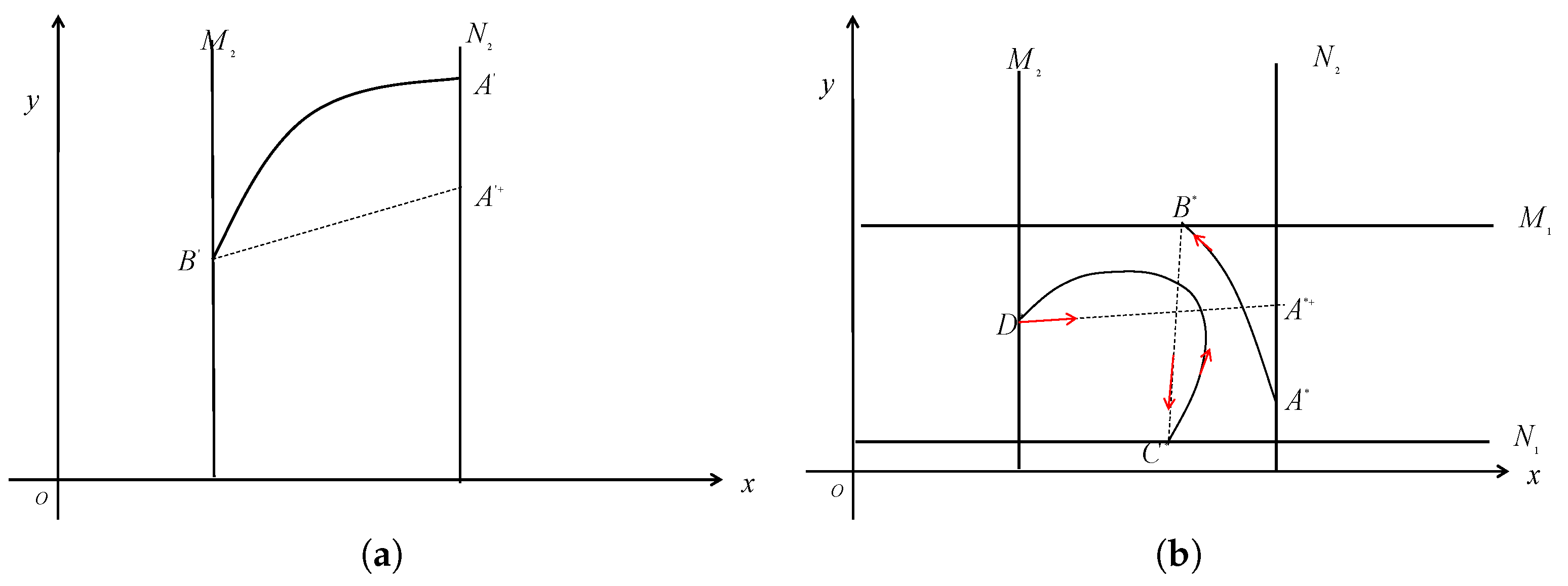
If the successor point of P is above point P, then the successor function $f\left(P\right)>0$, then it is necessary to find a point such that the corresponding successor function is less than 0. Choose a point $A_6$ away from the x-axis, then the trajectory through point $A_6$ intersects the impulsive set $M_2$, and it is mapped to point $A_6^{+}$, then the successor function $f\left(A_6\right)<0$. Then the existence of order-1 periodic solution is proved.

□

Figure 5. The existence of order-1 periodic solution of system (4).

Figure 5. The existence of order-1 periodic solution of system (4).

Remark 2. 

From Theorem 3, we can find that the economic collapse can be avoided through reasonable economic development ($q_1$). In addition, while rapidly developing the economy, it is necessary to pay attention to the problem of high cost of resources and environment.

In the following, we will discuss the existence of the order-2 periodic solution of system (2) for the case of $h_1<x_2^{*}<(1+q_1)h_1$, $(1-q_2)h_2<y_2^{*}<h_2$.

Theorem 4. 

If $y_{W_3}<y_D, x_B-{\tau }_2>x_{W_2}, y_I+{\tau }_2<y_{W_1}$, then there is an order-2 periodic solution for system (2).

Proof. 

Assume that the trajectory $l_6$ from $W_2$ is tangent to the impulsive set $M_2$ at point $W_3$. We further assume that point $A(x_A,y_A)\in N_2$ is the intersection point of curve $l_2$ and the phase set $N_2$, and point A is very close to the phase set $N_1$, i.e., $y_A=y_{W_2}+\epsilon$, then the trajectory starting from A intersects the impulsive set $M_1$ at point $B(x_B,y_B)\in M_1$. After that, it is mapped to point $C(x_C,y_C)\in N_1$, and it will intersect $M_2$ at point $D\in M_2$, due to impulsive effect, it is mapped to point $A^{+}$ which is the successor point of point A, then we have successor function $f\left(A\right)=y_D+\tau -y_A$. Since $y_D>y_{W_2}$, then $f\left(A\right)=y_D+\tau -y_{W_2}+\epsilon >0$.

It is necessary to find a point such that the corresponding successor function is less than 0. Assume that $W_1$ is the intersection point of the impulsive set $M_1$ and the phase set $N_2$, we choose a point $F\in N_2$ that is very close to point $W_1$, i.e., $y_{W_1}=y_F+\epsilon$, then the trajectory from point F intersects the impulsive set $M_1$ at point G, and it is mapped to point $H\in N_1$. After that, it intersects the impulsive set $M_2$ at point I, and it is mapped to point $F^{+}$, then we obtain that $f\left(F\right)=y_I+\tau -y_F=y_I+\tau -y_{W_1}+\epsilon <0$. Then there exists a point $S\in \overline{AF}$ such that $f\left(S\right)=0$, this means that system exists an order-2 periodic solution, as is shown in Figure 6. □

Remark 3. 

From Theorem 4, we can find that through reasonable pollution control and economy development ($q_1$, $q_2$, ${\tau }_1,{\tau }_2$), the pollution and capital will maintain a sustained and stable periodic change. Bilateral control can not only avoid causing high pollution, but also maintain stable economic development.

3.2.1. Stability of Order-1 Periodic Solution of System (3)

Let $({\xi }_1\left(t\right),{\omega }_1\left(t\right))$ be the order-1 periodic solution of system (3) with period $T_1$. In the following, the stability (see Definition A3 in Appendix A) will be proved, then we have the following Theorem 5.

Theorem 5. 

The order-1 periodic solution of system (3) is orbitally asymptotically stable if $|{\Delta }_1\rho |<1$ holds, where

$${\Delta }_1={\displaystyle \frac{\theta (1-u)\alpha x_A^2\left(t\right)-{\delta }_2(1-q_2)h_2(1+\alpha x_A^2\left(t\right))}{\theta (1-u)\alpha x_A^2\left(t\right)-{\delta }_2{h}_2(1+\alpha x_A^2\left(t\right))}},$$

and

$$\rho =exp\left\{{\int }_{0^{+}}^{T_1}\left({\displaystyle \frac{s(1-u)\alpha (1-\alpha x^2\left(t\right))}{{(1+x^2\left(t\right))}^2}}-{\delta }_2\right)\mathrm{d}t\right\}.$$

Proof. 

Define

$$\begin{array}{cc}\hfill & g_1(x,y)={\displaystyle \frac{s(1-u)\alpha x^2\left(t\right)}{(1+by\left(t\right))(1+\alpha x^2\left(t\right))}}-{\delta }_{1}x\left(t\right),g_2(x,y)={\displaystyle \frac{\theta (1-u)\alpha x^2\left(t\right)}{1+\alpha x^2\left(t\right)}}-{\delta }_{2}y\left(t\right),\hfill \\ \hfill & {\displaystyle \frac{\partial g_1(x,y)}{\partial x}}={\displaystyle \frac{2s\alpha (1-u)x}{(1+by){(1+\alpha x^2)}^2}}-{\delta }_1,{\displaystyle \frac{\partial g_2(x,y)}{\partial y}}=-{\delta }_2,{\phi }_1(x,y)=y-h_2,\hfill \\ \hfill & {\eta }_1(x,y)=0,{\eta }_2(x,y)=-q_{2}y,{\displaystyle \frac{\partial {\eta }_1}{\partial x}}=0,{\displaystyle \frac{\partial {\eta }_1}{\partial y}}=0,{\displaystyle \frac{\partial {\eta }_2}{\partial x}}=0,{\displaystyle \frac{\partial {\eta }_2}{\partial y}}=-q_2,\hfill \\ \hfill & {\displaystyle \frac{\partial {\phi }_1}{\partial x}}=0,{\displaystyle \frac{\partial {\phi }_1}{\partial y}}=1.\hfill \end{array}$$

By a simple calculation, we can obtain:

$$\begin{array}{cc}\hfill {\Delta }_1=& {\displaystyle \frac{g_{1+}(\frac{\partial {\eta }_1}{\partial y}\frac{\partial {\phi }_1}{\partial x}-\frac{\partial {\eta }_1}{\partial x}\frac{\partial {\phi }_1}{\partial y}+\frac{\partial {\phi }_1}{\partial x})+g_{2+}(\frac{\partial {\eta }_2}{\partial x}\frac{\partial {\phi }_1}{\partial y}-\frac{\partial {\eta }_2}{\partial y}\frac{\partial {\phi }_1}{\partial x}+\frac{\partial {\phi }_1}{\partial y})}{g_1\left(\frac{\partial {\phi }_1}{\partial x}\right)+g_2\left(\frac{\partial {\phi }_1}{\partial y}\right)}}\hfill \\ \hfill =& {\displaystyle \frac{g_{2+}({\xi }_1(T_1+0),{\omega }_1(T_1+0))}{g_2({\xi }_1(T+0),{\omega }_1(T+0))}},\hfill \\ \hfill =& {\displaystyle \frac{\theta (1-u)\alpha x_A^2\left(t\right)-{\delta }_2(1-q_2)h_2(1+\alpha x_A^2\left(t\right))}{\theta (1-u)\alpha x_A^2\left(t\right)-{\delta }_2{h}_2(1+\alpha x_A^2\left(t\right))}}.\hfill \end{array}$$

$$\begin{array}{cc}\hfill {\int }_{0^{+}}^{T_1}\left({\displaystyle \frac{\partial g_1}{\partial x}}+{\displaystyle \frac{\partial g_2}{\partial y}}\right)\mathrm{d}t=& {\int }_{0^{+}}^{T_1}\left({\displaystyle \frac{s(1-u)\alpha x\left(t\right)}{(1+by\left(t\right)){(1+x^2\left(t\right))}^2}}-{\delta }_1\right)\mathrm{d}t\hfill \\ \hfill & +{\int }_{0^{+}}^{T_1}\left({\displaystyle \frac{s(1-u)\alpha (1-\alpha x^2\left(t\right))}{{(1+x^2\left(t\right))}^2}}-{\delta }_2\right)\mathrm{d}t\hfill \\ \hfill =& {\int }_{x_A}^{x_B}{\displaystyle \frac{1}{x}}\mathrm{d}x+{\int }_{0^{+}}^{T_1}\left({\displaystyle \frac{s(1-u)\alpha (1-\alpha x^2\left(t\right))}{{(1+x^2\left(t\right))}^2}}-{\delta }_2\right)\mathrm{d}t\hfill \\ \hfill =& ln{\displaystyle \frac{x_{B_1}}{x_{A_1}}}+{\int }_{0^{+}}^{T_1}\left({\displaystyle \frac{s(1-u)\alpha (1-\alpha x^2\left(t\right))}{{(1+x^2\left(t\right))}^2}}-{\delta }_2\right)\mathrm{d}t.\hfill \end{array}$$

$$\begin{array}{cc}\hfill {\mu }_2=& {\Delta }_1{\displaystyle \frac{x_{B_1}}{x_{A_1}}}exp\left\{{\int }_{0^{+}}^{T_1}\left({\displaystyle \frac{s(1-u)\alpha (1-\alpha x^2\left(t\right))}{{(1+x^2\left(t\right))}^2}}-{\delta }_2\right)\right\}={\Delta }_1\rho ,\hfill \end{array}$$

where

$$\rho ={\displaystyle \frac{x_{B_1}}{x_{A_1}}}exp\left\{{\int }_{0^{+}}^{T_1}\left({\displaystyle \frac{s(1-u)\alpha (1-\alpha x^2\left(t\right))}{{(1+x^2\left(t\right))}^2}}-{\delta }_2\right)\mathrm{d}t\right\}.$$

If $|{\Delta }_1\rho |<1$, then $|{\mu }_2|<1$, the result can be obtained. □

Remark 4. 

In the same manner, the stability of order-1 periodic solution of system (4) can be proved, so we omit it here.

3.2.2. Stability of the Order-2 Periodic Solution

Let $T\left(t\right)=\left(\xi \right(t),\omega (t\left)\right)$ be the order-2 periodic solution of system (2). We will prove the stability of the order-2 periodic solution of system (2).

Theorem 6. 

The order-2 periodic solution of system (2) is orbitally asymptotically stable if $|{\mathrm{\Phi }}_1|<1$ holds, where

$$\begin{array}{cc}\hfill & {\mathrm{\Phi }}_1={\Delta }_1{\Delta }_2{\displaystyle \frac{x_B{x}_D}{x_A{x}_C}}\left\{{\int }_{0^{+}}^{T_1+T_2}\left({\displaystyle \frac{s(1-u)\alpha (1-\alpha x^2\left(t\right))}{{(1+x^2\left(t\right))}^2}}-{\delta }_2\right)\mathrm{d}t\right\},\hfill \\ \hfill & {\Delta }_1={\displaystyle \frac{\theta (1-u)\alpha x_A^2\left(t\right)-{\delta }_2(1-q_2)h_2(1+\alpha x_A^2\left(t\right))}{\theta (1-u)\alpha x_A^2\left(t\right)-{\delta }_2{h}_2(1+\alpha x_A^2\left(t\right))}},\hfill \\ \hfill & {\Delta }_2={\displaystyle \frac{s(1-u)\alpha {(1+q_1)}^2{h}_1^2-{\delta }_1{h}_1(1+b(y_D+\tau ))(1+\alpha h_1^2{(1+q_1)}^2)}{s(1-u)\alpha h_1^2-{\delta }_1{h}_1(1+b{y}_D)(1+\alpha h_1^2)}}.\hfill \end{array}$$

Proof. 

Based on system (2), we can obtain:

$$\begin{array}{cc}\hfill & g_1(x,y)={\displaystyle \frac{s(1-u)\alpha x^2\left(t\right)}{(1+by\left(t\right))(1+\alpha x^2\left(t\right))}}-{\delta }_{1}x\left(t\right),g_2(x,y)={\displaystyle \frac{\theta (1-u)\alpha x^2\left(t\right)}{1+\alpha x^2\left(t\right)}}-{\delta }_{2}y\left(t\right),\hfill \\ \hfill & {\displaystyle \frac{\partial g_1(x,y)}{\partial x}}={\displaystyle \frac{2s\alpha (1-u)x}{(1+by){(1+\alpha x^2)}^2}}-{\delta }_1,{\displaystyle \frac{\partial g_2(x,y)}{\partial y}}=-{\delta }_2,{\phi }_1(x,y)=y-h_2,{\eta }_1(x,y)=0,\hfill \\ \hfill & {\eta }_2(x,y)=-q_{2}y,{\displaystyle \frac{\partial {\eta }_1}{\partial x}}=0,{\displaystyle \frac{\partial {\eta }_1}{\partial y}}=0,{\displaystyle \frac{\partial {\eta }_2}{\partial x}}=0,{\displaystyle \frac{\partial {\eta }_2}{\partial y}}=-q_2,{\displaystyle \frac{\partial {\phi }_1}{\partial x}}=0,{\displaystyle \frac{\partial {\phi }_1}{\partial y}}=1,\hfill \\ \hfill & {\phi }_2(x,y)=x-h_1,{\eta }_3(x,y)=q_{1}x,{\eta }_4(x,y)=0,{\displaystyle \frac{\partial {\eta }_3}{\partial x}}=q_1,{\displaystyle \frac{\partial {\eta }_3}{\partial y}}=0,{\displaystyle \frac{\partial {\eta }_4}{\partial x}}=0,\hfill \\ \hfill & {\displaystyle \frac{\partial {\eta }_4}{\partial y}}=0,{\displaystyle \frac{\partial {\phi }_2}{\partial x}}=1,{\displaystyle \frac{\partial {\phi }_2}{\partial y}}=0.\hfill \end{array}$$

By simple calculation,

$$\begin{array}{cc}\hfill {\Delta }_1=& {\displaystyle \frac{g_{1+}(\frac{\partial {\eta }_1}{\partial y}\frac{\partial {\phi }_1}{\partial x}-\frac{\partial {\eta }_1}{\partial x}\frac{\partial {\phi }_1}{\partial y}+\frac{\partial {\phi }_1}{\partial x})+g_{2+}(\frac{\partial {\eta }_2}{\partial x}\frac{\partial {\phi }_1}{\partial y}-\frac{\partial {\eta }_2}{\partial y}\frac{\partial {\phi }_1}{\partial x}+\frac{\partial {\phi }_1}{\partial y})}{g_1\left(\frac{\partial {\phi }_1}{\partial x}\right)+g_2\left(\frac{\partial {\phi }_1}{\partial y}\right)}}\hfill \\ \hfill =& {\displaystyle \frac{g_{2+}(\xi (T_1+0),\omega (T_1+0))}{g_2(\xi (T_1+0),\omega (T_1+0))}},\hfill \\ \hfill =& {\displaystyle \frac{\theta (1-u)\alpha x_A^2\left(t\right)-{\delta }_2(1-q_2)h_2(1+\alpha x_A^2\left(t\right))}{\theta (1-u)\alpha x_A^2\left(t\right)-{\delta }_2{h}_2(1+\alpha x_A^2\left(t\right))}},\hfill \end{array}$$

$$\begin{array}{cc}\hfill {\Delta }_2=& {\displaystyle \frac{g_{1+}(\frac{\partial {\eta }_2}{\partial y}\frac{\partial {\phi }_2}{\partial x}-\frac{\partial {\eta }_2}{\partial x}\frac{\partial {\phi }_2}{\partial y}+\frac{\partial {\phi }_2}{\partial x})+g_{2+}(\frac{\partial {\eta }_2}{\partial x}\frac{\partial {\phi }_2}{\partial y}-\frac{\partial {\eta }_2}{\partial y}\frac{\partial {\phi }_2}{\partial x}+\frac{\partial {\phi }_2}{\partial y})}{g_1\left(\frac{\partial {\phi }_2}{\partial x}\right)+g_2\left(\frac{\partial {\phi }_2}{\partial y}\right)}}\hfill \\ \hfill =& {\displaystyle \frac{g_{1+}(\xi (T_2+0),\omega (T_2+0))}{g_1(\xi (T_2+0),\omega (T_2+0))}},\hfill \\ \hfill =& {\displaystyle \frac{s(1-u)\alpha {(1+q_1)}^2{h}_1^2-{\delta }_1{h}_1(1+b(y_D+\tau ))(1+\alpha h_1^2{(1+q_1)}^2)}{s(1-u)\alpha h_1^2-{\delta }_1{h}_1(1+b{y}_D)(1+\alpha h_1^2)}},\hfill \end{array}$$

and

$$\begin{array}{cc}\hfill & {\int }_{0^{+}}^{T_1+T_2}\left({\displaystyle \frac{\partial g_1}{\partial x}}+{\displaystyle \frac{\partial g_2}{\partial y}}\right)\mathrm{d}t={\int }_{0^{+}}^{T_1+T_2}\left({\displaystyle \frac{s(1-u)\alpha x\left(t\right)}{(1+by\left(t\right)){(1+x^2\left(t\right))}^2}}-{\delta }_1\right)\mathrm{d}t\hfill \\ \hfill & +{\int }_{0^{+}}^{T_1+T_2}\left({\displaystyle \frac{s(1-u)\alpha (1-\alpha x^2\left(t\right))}{{(1+x^2\left(t\right))}^2}}-{\delta }_2\right)\mathrm{d}t\hfill \\ \hfill =& {\int }_{x_A}^{x_B}{\displaystyle \frac{1}{x}}\mathrm{d}x+{\int }_{x_C}^{x_D}{\displaystyle \frac{1}{x}}\mathrm{d}x+{\int }_{0^{+}}^{T_1+T_2}\left({\displaystyle \frac{s(1-u)\alpha (1-\alpha x^2\left(t\right))}{{(1+x^2\left(t\right))}^2}}-{\delta }_2\right)\mathrm{d}t\hfill \\ \hfill =& ln{\displaystyle \frac{x_B{x}_D}{x_A{x}_C}}+{\int }_{0^{+}}^{T_1+T_2}\left({\displaystyle \frac{s(1-u)\alpha (1-\alpha x^2\left(t\right))}{{(1+x^2\left(t\right))}^2}}-{\delta }_2\right)\mathrm{d}t.\hfill \end{array}$$

Then we have

$$\begin{array}{cc}\hfill {\mu }_2=& {\Delta }_1{\Delta }_{2}exp\left\{{\int }_{0^{+}}^{T_1+T_2}\left({\displaystyle \frac{\partial P}{\partial x}}+{\displaystyle \frac{\partial Q}{\partial y}}\right)\mathrm{d}t\right\}\hfill \\ \hfill =& {\Delta }_1{\Delta }_2{\displaystyle \frac{x_B{x}_D}{x_A{x}_C}}\left\{{\int }_{0^{+}}^{T_1+T_2}\left({\displaystyle \frac{s(1-u)\alpha (1-\alpha x^2\left(t\right))}{{(1+x^2\left(t\right))}^2}}-{\delta }_2\right)\mathrm{d}t\right\}\hfill \\ \hfill =& :{\mathrm{\Phi }}_1.\hfill \end{array}$$

If $|{\mathrm{\Phi }}_1|<1$, then $|{\mu }_2|<1$; thus the result is obtained. □

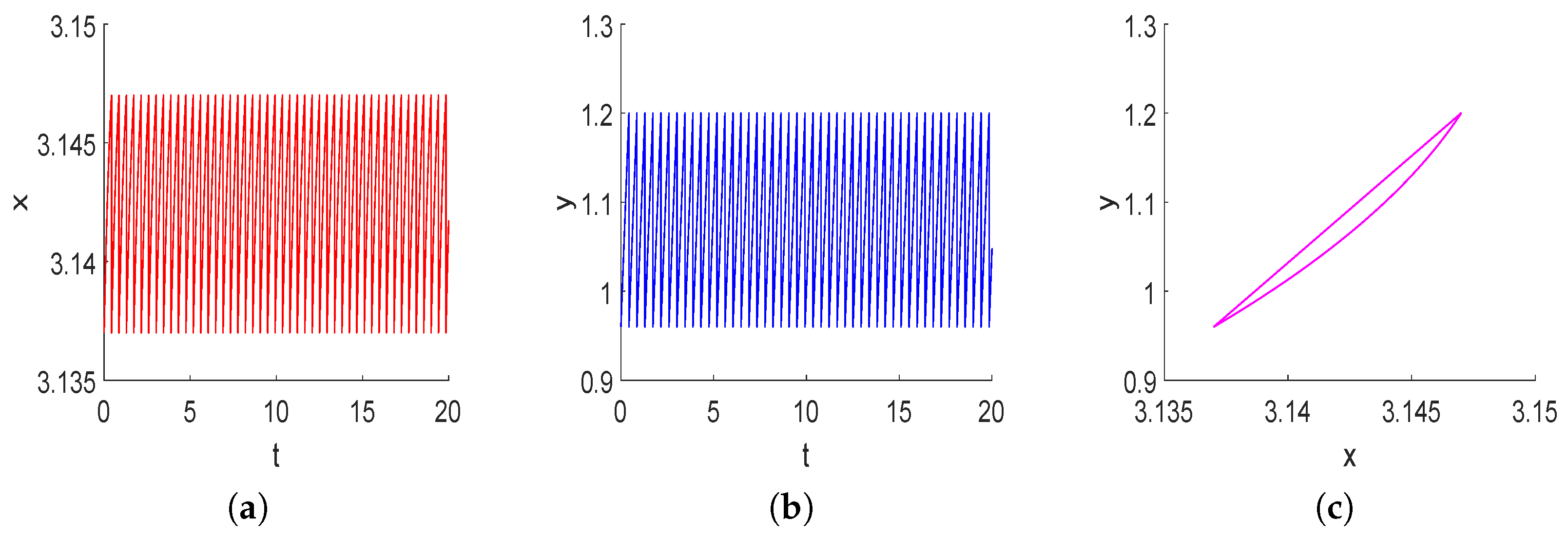
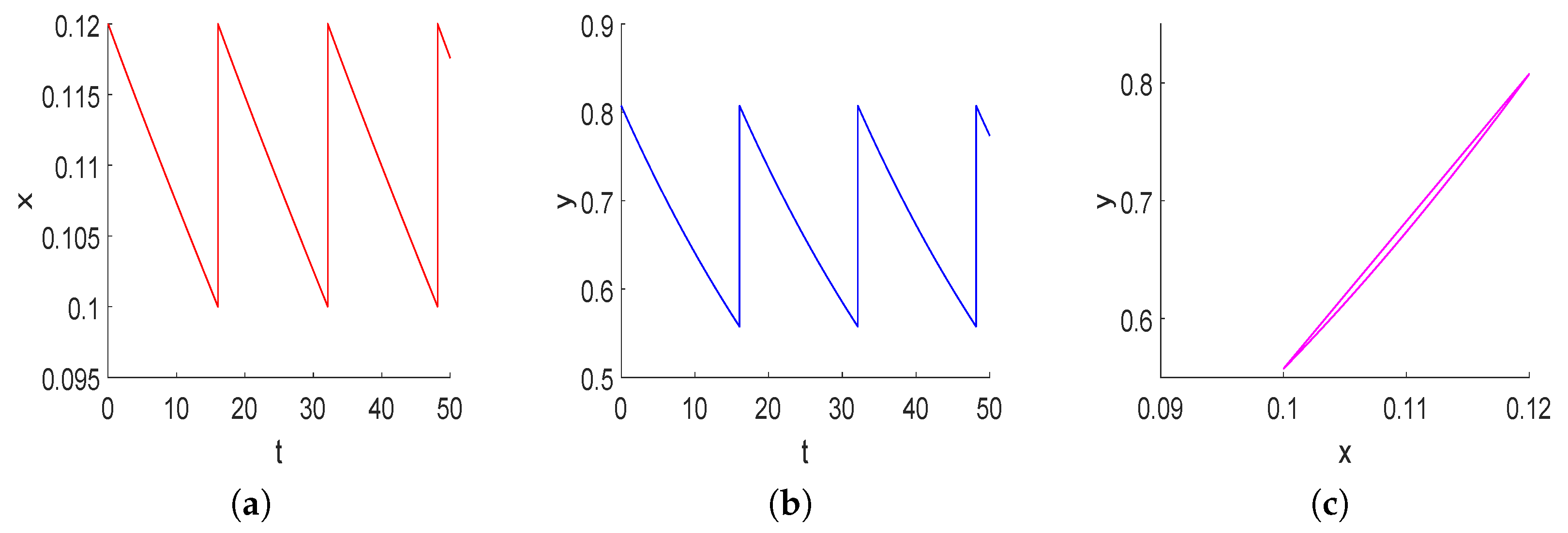
4. Numerical Simulations

In this section, we perform some numerical simulations to prove the validity of the theoretical results in the previous sections. The model parameters are listed as follows [17]:

$$\begin{array}{c}\hfill {\delta }_1=0.05,{\delta }_2=0.04,\theta =0.8,b=1,\alpha =1.5,s=0.5.\end{array}$$

Example 1. 

To illustrate the existence of order-1 periodic solution of system (3), the specific system is given by:

$$\left\{\begin{array}{c}\left.\begin{array}{c}{\displaystyle \frac{\mathrm{d}x}{\mathrm{d}t}}={\displaystyle \frac{0.5\times (1-0.2)1.5x^2\left(t\right)}{(1+y\left(t\right))(1+1.5x^2\left(t\right))}}-0.05x\left(t\right)\hfill \\ {\displaystyle \frac{\mathrm{d}y}{\mathrm{d}t}}={\displaystyle \frac{0.8\times (1-0.2)\times 1.5x^2\left(t\right)}{1+1.5x^2\left(t\right)}}-0.04y\left(t\right)\hfill \end{array}\right\}y<h_2,\hfill \\ \left.\begin{array}{c}\Delta x=-{\tau }_2\hfill \\ \Delta y=-q_{2}y\hfill \end{array}\right\}y=h_2\hfill \end{array}\right.$$

For the case of $(1-q_2)h_2<h_2<y_2^{*}$, we choose the control parameters: $h_2=1.2,{\tau }_2=0.05$, $p_2=0.2$, system (3) exists an order-1 periodic solution (see Figure 7), this corresponds to the second case of Theorem 1.

Keep other parameters unchanged but ${\tau }_2=0.01$, the trajectory starting from the point $(3.1370, 0.96)$, then system (3) also exists an order-1 periodic solution (see Figure 8). This corresponds to the third case of Theorem 1.

Now, we show that there exists order-1 periodic solution of system (3) for the case of $(1-q_2)h_2<y_2^{*}<h_2$. Keep the model parameters unchanged, we choose the control parameters $p_2=0.2,h_2=3,{\tau }_2=0.02$, then we find that system (3) exists order-1 periodic solution (see Figure 9).

Keep the other parameters unchanged, the trajectory will approach the origin point as ${\tau }_2$ increases. This means that the negative impact on economic development in the process of pollution control is serious, it will also lead to economic collapse. This reminds us that pollution control and economic development need to be synchronized.

Example 2. 

In the following, we will show that there exists an order-1 periodic solution of system (4) for the case of $x_1^{*}<(1-q_1)h_1<h_1<x_2^{*}$. Here, we choose the control parameters: $p_1=0.2$, ${\tau }_1=0.01,h_1=0.1$. Then we have the following specific system:

$$\left\{\begin{array}{c}\left.\begin{array}{c}{\displaystyle \frac{\mathrm{d}x}{\mathrm{d}t}}={\displaystyle \frac{0.5\times (1-0.2)x^2\left(t\right)}{(1+y\left(t\right))(1+1.5x^2\left(t\right))}}-0.05x\left(t\right)\hfill \\ {\displaystyle \frac{\mathrm{d}y}{\mathrm{d}t}}={\displaystyle \frac{0.8(1-0.2)\times 1.5x^2\left(t\right)}{1+1.5x^2\left(t\right)}}-0.04y\left(t\right)\hfill \end{array}\right\}x>0.1,\hfill \\ \left.\begin{array}{c}\Delta x=0.1x\hfill \\ \Delta y=0.05\hfill \end{array}\right\}x=0.1.\hfill \end{array}\right.$$

By numerical simulations, we find that the trajectory starting from point $(0.22, 0.6709)$, then system (4) exists an order-1 periodic solution, as is shown in Figure 10. Through reasonable economic development, then the economic collapse can be avoided. In addition, it is necessary to pay attention to the problem of high cost of resources and environment while developing the economy.

Example 3. 

To illustrate the existence of order-2 periodic solution of system (2) in Section 2, the specific system is given by:

$$\left\{\begin{array}{c}\left.\begin{array}{c}{\displaystyle \frac{\mathrm{d}x}{\mathrm{d}t}}={\displaystyle \frac{0.5\times (1-0.2)\times 1.5x^2\left(t\right)}{(1+y\left(t\right))(1+1.5x^2\left(t\right))}}-0.05x\left(t\right)\hfill \\ {\displaystyle \frac{\mathrm{d}y}{\mathrm{d}t}}={\displaystyle \frac{0.8\times (1-0.2)\times 1.5x^2\left(t\right)}{1+1.5x^2\left(t\right)}}-0.04y\left(t\right)\hfill \end{array}\right\}x>0.36,y<4,\hfill \\ \left.\begin{array}{c}\Delta x=0.6x,\Delta y=0.05\hfill \end{array}\right\}x=0.36,\hfill \\ \left.\begin{array}{c}\Delta x=-0.1,\Delta y=-0.2y\hfill \end{array}\right\}y=4.\hfill \end{array}\right.$$

(5)

We choose control parameters: $h_1=0.36,h_2=4,q_1=0.6,q_2=0.2$, ${\tau }_1=0.05$ and ${\tau }_2=0.15$. It is easily observed that system (2) exists an order-2 periodic solution (see Figure 11). Also, we find that the bilateral control can not only avoid high pollution, but also ensure the stable development of economy.

5. Conclusions

In this paper, for the sustainable development of economy, we develop an economic-environment model with unilateral and bilateral control. We study the existence and stability of order-1 periodic solution and order-2 periodic solution of unilateral system and bilateral system, respectively. Numerical simulations are performed to verify the validity of the theoretical results. On the one hand, when the upper threshold of the density of pollution is limited, through reasonable control of pollution, then high pollution can be avoided. In addition, if the negative impact on economic development in the process of pollution control is serious, it will also lead to economic collapse. On the other hand, when the lower threshold of the number of the capital is limited, through reasonable economic development, then the economic collapse can be avoided. However, it is necessary to pay attention to the problem of high cost of resources and environment while rapidly developing the economy. This reminds us that economic development and pollution control need to be synchronized. Besides, compared with the two unilateral system, the bilateral system is more effective to maintain the sustainable economic development.

This research aims to enrich nonlinear research in sustainable development through mathematical modeling, with the goal of providing scientific insights to support government decision-making in advancing sustainable development.

References

- McGlade, C.; Ekins, P. The geographical distribution of fossil fuels unused when limiting global warming to 2 °C. Nature 2015, 554, 229–233. [Google Scholar] [CrossRef] [PubMed]
- Sadr, N.; Bahrdo, T.; Taghizadeh, R. Impacts of Paris agreement, fossil fuel consumption, and net energy imports on CO2 emissions: A panel data approach for three West European countries. Clean Technol. Environ. Policy 2022, 24, 1521–1534. [Google Scholar] [CrossRef]
- Li, Y.; Wu, H.; Shen, K.; Hao, Y.; Zhang, P. Is environmental pressure distributed equally in China? Empirical evidence from provincial and industrial panel data analysis. Sci. Total Environ. 2020, 718, 137363. [Google Scholar] [CrossRef]
- Jia, J.; Xin, L.; Lu, C.; Wu, B.; Zhong, Y. China’s CO2 emissions: A systematical decomposition concurrently from multi-sectors and multi-stages since 1980 by an extended logarithmic mean divisia index. Energy Strateg. Rev. 2023, 49, 101141. [Google Scholar] [CrossRef]
- Zhao, B.; Wang, S.; Hao, J. Challenges and perspectives of air pollution control in China. Front. Env. Sci. Eng. 2024, 18, 68. [Google Scholar] [CrossRef]
- Lei, Y.; Yin, Z.; Lu, X.; Zhang, Q.; Gong, J.; Cai, B.; Cai, C.; Chai, Q.; Chen, H.; Chen, R.; et al. The 2022 report of synergetic roadmap on carbon neutrality and clean air for China: Accelerating transition in key sectors. Environ. Sci. Ecotechnol. 2024, 19, 100335. [Google Scholar] [CrossRef]
- Weichenthal, S.; Pinault, L.; Christidis, T.; Burnett, R.T.; Brook, J.R.; Chu, Y.; Crouse, D.L.; Erickson, A.C.; Hystad, P.; Li, C.; et al. How low can you go? Air pollution affects mortality atvery low levels. Sci. Adv. 2022, 8, eabo3381. [Google Scholar] [CrossRef]
- Li, R.; Li, L.; Wang, Q. The impact of energy efficiency on carbon emissions: Evidence from the transportation sector in Chinese 30 provinces. Sustain. Cities Soc. 2022, 82, 103880. [Google Scholar] [CrossRef]
- Wang, M.; Feng, C. The win-win ability of environmental protection and economic development during China’s transition. Technol. Forecast. Social Change 2021, 166, 120617. [Google Scholar] [CrossRef]
- Brock, W.A. Economics of Natural and Environmental Resources; Gordon & Breach: New York, NY, USA, 1973. [Google Scholar]
- Mäler, K.G. Environmental Economics: A Theoretical Inquiry; Johns Hopkins University Press: Baltimore, MD, USA, 1974. [Google Scholar]
- Nordhaus, W.D. An optimal transition path for controlling greenhouse gases. Science 1992, 258, 1315–1319. [Google Scholar] [CrossRef]
- Nordhaus, W.D. A Question of Balance: Economic Modeling of Global Warming; Yale University Press: New Haven, CT, USA, 2008. [Google Scholar]
- La Torre, D.; Liuzzi, D.; Marsiglio, S. Pollution diffusion and abatement activities across space and over time. Math. Soc. Sci. 2015, 78, 48–63. [Google Scholar] [CrossRef]
- Capasso, V.; Engbers, R.; Torre, D.L. On a spatial Solow model with technological diffusion and nonconcave production function. Nonlinear Anal. Real World Appl. 2010, 11, 3858–3876. [Google Scholar] [CrossRef]
- Skiba, A.K. Optimal growth with a convex-concave production function. Econometrica 1978, 46, 527–539. [Google Scholar] [CrossRef]
- Liuzzi, D.; Venturi, B. Pollution-induced poverty traps via Hopf bifurcation in a minimal integrated economic-environment model. Commun. Nonlinear. Sci. 2021, 93, 105523. [Google Scholar] [CrossRef]
- Sun, D.; Zeng, S.; Lin, H.; Meng, X.; Yu, B. Can transport infrastructure pave a green way? A city-level examination in China. J. Clean. Prod. 2019, 226, 669–678. [Google Scholar] [CrossRef]
- Enyoh, C.E.; Verla, A.W.; Wang, Q.; Ohiagu, F.O.; Chowdhury, A.H.; Enyoh, E.C.; Chowdhury, T.; Verla, E.N.; Chinwendu, U.P. An overview of emerging pollutants in air: Method of analysis and potential public health concern from human environmental exposure. Trends Environ. Anal. Chem. 2020, 28, e00107. [Google Scholar] [CrossRef]
- Liu, S.; Tian, H.; Zhu, C. Reduced but still noteworthy atmospheric pollution of trace elements in China. One Earth 2023, 6, 536–547. [Google Scholar] [CrossRef]
- Sun, K.; Zhang, T.; Tian, Y. Theoretical study and control optimization of an integrated pest management predator–prey model with power growth rate. Math. Biosci. 2016, 279, 13–26. [Google Scholar] [CrossRef]
- Sun, K.; Zhang, T.; Tian, Y. Dynamics analysis and control optimization of a pest management predator–prey model with an integrated control strategy. Appl. Math. Comput. 2017, 292, 253–271. [Google Scholar] [CrossRef]
- Song, X.; Huang, M.; Li, J. Modeling impulsive insulin delivery in insulin pump with time delays. SIAM J. Appl. Math. 2014, 74, 1763–1785. [Google Scholar] [CrossRef]
- Guo, H.; Tian, Y.; Sun, K. Study on dynamic behavior of two fishery harvesting models: Effects of variable prey refuge and imprecise biological parameters. J. Appl. Math. Comput. 2023, 69, 4243–4268. [Google Scholar]
- Tian, Y.; Guo, H.; Sun, K. Complex dynamics of two prey-predator harvesting models with prey refuge and interval-valued imprecise parameters. Math. Methods Appl. Sci. 2023, 46, 14278–14298. [Google Scholar] [CrossRef]
- Xu, J.; Huang, M.; Song, X. Dynamics of a guanaco-sheep competitive system with unilateral and bilateral control. Nonlinear Dyn. 2022, 107, 3111–3126. [Google Scholar] [CrossRef]
- Zhang, M.; Zhao, Y.; Song, X. Dynamics of bilateral control system with state feedback for price adjustment strategy. Int. J. Biomath. 2021, 14, 2150031. [Google Scholar] [CrossRef]
- Yu, H.; Lin, X. Study of environmental pollution control investment efficiency and its influence in Beijing-Tianjin-Hebei region. Ind. Technol. Econ. 2018, 5, 138–146. [Google Scholar]
- Zhao, X.; Long, L.; Sun, Q. How to Evaluate Investment Efficiency of Environmental Pollution Control: Evidence from China. Int. J. Environ. Res. Public Health 2022, 19, 7252. [Google Scholar] [CrossRef]
- Feng, Q.; Sun, T. Comprehensive evaluation of benefits from environmental investment: Take China as an example. Environ. Sci. Pollut. Res. 2020, 27, 15292–15304. [Google Scholar] [CrossRef] [PubMed]
- Xiang, L.; Zhang, H.; Lyu, Y. A Study on the Impact of Reform and Opening-up on Sustainable Development: Evidence from China. Probl. Ekorozw. 2023, 18, 204–215. [Google Scholar] [CrossRef]
- Bainov, D.; Simeonov, P.S. Impulsive Differential Equations: Periodic Solutions and Applications; Routledge: New York, NY, USA, 1993; Volume 66. [Google Scholar]
- Simeonov, P.S.; Bainov, D.D. Orbital stability of periodic solutions of autonomous systems with impulse effect. Int. J. Syst. Sci. 1989, 19, 2561–2585. [Google Scholar] [CrossRef]
Disclaimer/Publisher’s Note: The statements, opinions and data contained in all publications are solely those of the individual author(s) and contributor(s) and not of MDPI and/or the editor(s). MDPI and/or the editor(s) disclaim responsibility for any injury to people or property resulting from any ideas, methods, instructions or products referred to in the content. |
© 2025 by the authors. Licensee MDPI, Basel, Switzerland. This article is an open access article distributed under the terms and conditions of the Creative Commons Attribution (CC BY) license (https://creativecommons.org/licenses/by/4.0/).
Share and Cite
Xu, J.; Huang, M.; Yang, J. Dynamical Analysis of an Economic-Environment Model with Unilateral and Bilateral Control. Mathematics 2025, 13, 1268. https://doi.org/10.3390/math13081268
Xu J, Huang M, Yang J. Dynamical Analysis of an Economic-Environment Model with Unilateral and Bilateral Control. Mathematics. 2025; 13(8):1268. https://doi.org/10.3390/math13081268
Chicago/Turabian StyleXu, Jing, Mingzhan Huang, and Jingen Yang. 2025. "Dynamical Analysis of an Economic-Environment Model with Unilateral and Bilateral Control" Mathematics 13, no. 8: 1268. https://doi.org/10.3390/math13081268
APA StyleXu, J., Huang, M., & Yang, J. (2025). Dynamical Analysis of an Economic-Environment Model with Unilateral and Bilateral Control. Mathematics, 13(8), 1268. https://doi.org/10.3390/math13081268