Truncated-Exponential-Based General-Appell Polynomials

Abstract

In this paper, a new and general form of truncated-exponential-based general-Appell polynomials is introduced using the two-variable general-Appell polynomials. For this new polynomial family, we present an explicit representation, recurrence relation, shift operators, differential equation, determinant representation, and some other properties. Finally, two special cases of this family, truncated-exponential-based Hermite-type and truncated-exponential-based Laguerre–Frobenius Euler polynomials, are introduced and their corresponding properties are obtained.

1. Introduction

In applied sciences, engineering, physics, mathematics, and other relevant research domains, truncated polynomials are extensively utilized. They have been demonstrated to be crucial for the assessment of integrals involving the multiplication of special functions, which are significant in a variety of domains. Also, truncated versions of special polynomials have been extensively researched and analyzed by mathematicians. For example, Dattoli et al. [1] presented higher-order truncated polynomials that are useful for analyzing integrals involving special functions. Srivastava et al. [2] studied Apostol-type polynomials with a truncated exponential basis and gave their various properties. Duran and Açıkgöz [3] defined truncated Fubini polynomials of two variables and their numbers, and later, they studied degenerate truncated special polynomials in [4]. Kumam et al. defined truncated-exponential-based Frobenius–Euler polynomials in [5]. Then, Raza et al. [6] defined the q-truncated-exponential polynomials. In [7], Costabile et al. defined q-truncated-exponential-Appell polynomials and provided their fundamental properties. Special polynomials and numbers have been the subject of recent study among mathematicians due to their applications, such as quasi-monomiality characteristics, differential equations, and integral representations.

For each $e^x$, the first $\left(j+1\right)$ terms of the Maclaurin series are the truncated exponential polynomials $e_j\left(x\right)$ [8] defined by the series

$$e_j\left(x\right)=\sum _{k=0}^j{\displaystyle \frac{x^k}{k!}}.$$

Dattoli et al. [1] provide an analysis of these polynomials characteristics. The generating function of the truncated exponential polynomials in [1] is

$${\displaystyle \frac{1}{1-t}}{e}^{xt}=\sum _{j=0}^{\infty }{e}_j\left(x\right)t^j.$$

(1)

The two-variable form of truncated-exponential polynomials in [1] is given by the following explicit notation:

$${\phantom{­}}_{\left[2\right]}{e}_j\left(x,y\right)=\sum _{k=0}^{\left[\frac{j}{2}\right]}{\displaystyle \frac{y^k{x}^{j-2k}}{\left(j-2k\right)!}}$$

(2)

and the generating function in [1] is as follows

$$\sum _{j=0}^{\infty }{\phantom{­}}_{\left[2\right]}{e}_j\left(x,y\right)t^j=e^{xt}{\displaystyle \frac{1}{1-y{t}^2}}.$$

(3)

The following series defines truncated polynomials ${\phantom{­}}_{\left[2\right]}{e}_j\left(x,y\right)$ of two variables of order m in [9], which we investigate in order to present a hybrid family of special polynomials related to Appell sequences:

$$e_j^{\left(m\right)}\left(x,y\right)=\sum _{k=0}^{\left[\frac{j}{m}\right]}{\displaystyle \frac{y^k{x}^{j-mk}}{\left(j-mk\right)!}}$$

(4)

with the following generating function

$$\sum _{j=0}^{\infty }{e}_j^{\left(m\right)}\left(x,y\right)t^j=e^{xt}{\displaystyle \frac{1}{1-y{t}^m}}.$$

(5)

The identity ${\displaystyle \frac{d}{dx}}{\mathcal{A}}_j\left(x\right)=j{\mathcal{A}}_{j-1}\left(x\right),$ with ${\mathcal{A}}_0\left(x\right)\ne 0$ defines Appell polynomials, which are one of fundamental polynomials in special function theory. Bernoulli and Euler polynomials are the most well-known Appell polynomials. They can be defined using the generating relation [10,11]

$$A\left(t\right)e^{xt}=\stackrel{\infty }{\sum _{j=0}}{\mathcal{A}}_j\left(x\right){\displaystyle \frac{t^j}{j!}},$$

(6)

where $A\left(t\right)$ is a formal power series, which is known as the determining function, given by

$$A\left(t\right)=\stackrel{\infty }{\sum _{j=0}}{A}_j{\displaystyle \frac{t^j}{j!}},A_0\ne 0.$$

(7)

Bivariate generalization of Appell polynomials has recently been unified by Khan and Raza [12] using the following definition:

$$A\left(t\right)e^{xt}\psi \left(y,t\right)=\stackrel{\infty }{\sum _{j=0}}{\phantom{­}}_{\mathcal{S}}{\mathcal{A}}_j\left(x,y\right){\displaystyle \frac{t^j}{j!}},$$

(8)

where

$$e^{xt}\psi \left(y,t\right)=\underset{r=0}{\sum ^{\infty }}{\mathcal{S}}_r\left(x,y\right){\displaystyle \frac{t^r}{r!}},{\mathcal{S}}_0\left(x,y\right)=1,$$

(9)

$$\psi \left(y,t\right)=\underset{k=0}{\sum ^{\infty }}{\psi }_k\left(y\right){\displaystyle \frac{t^k}{k!}},{\psi }_0\left(y\right)\ne 0$$

(10)

and $A\left(t\right)$ is the determining function given in (7).

On the other hand, operational techniques utilizing differential operators, which arise from the quasi-monomiality principle, are useful methods for various generalizations of polynomials. In [12], Khan and Raza used these techniques to define the following multiplicative and derivative operators for general polynomials ${\mathcal{S}}_j\left(x,y\right)$ with two-variable in the light of the quasi monomiality principle:

$${\widehat{M}}_{\mathcal{S}}=x+{\displaystyle \frac{{\psi }^{\prime }\left(y,D_x\right)}{\psi \left(y,D_x\right)}}\mathrm{and}{\widehat{P}}_{\mathcal{S}}=D_x,\left(D_x:={\displaystyle \frac{\partial }{\partial x}},{\psi }^{\prime }\left(y,t\right):={\displaystyle \frac{\partial }{\partial t}}\psi \left(y,t\right)\right).$$

(11)

From [12], the polynomials ${\mathcal{S}}_j\left(x,y\right)$ have the following properties:

$$\begin{array}{ccc}\hfill {\widehat{M}}_{\mathcal{S}}\left\{{\mathcal{S}}_j\left(x,y\right)\right\}& =& {\mathcal{S}}_{j+1}\left(x,y\right),\hfill \end{array}$$

(12)

$$\begin{array}{ccc}\hfill {\widehat{P}}_{\mathcal{S}}\left\{{\mathcal{S}}_j\left(x,y\right)\right\}& =& j{\mathcal{S}}_{j-1}\left(x,y\right),\hfill \end{array}$$

(13)

$$\begin{array}{ccc}\hfill {\widehat{M}}_{\mathcal{S}}{\widehat{P}}_{\mathcal{S}}\left\{{\mathcal{S}}_j\left(x,y\right)\right\}& =& j{\mathcal{S}}_j\left(x,y\right),\hfill \end{array}$$

(14)

$$\begin{array}{ccc}\hfill exp\left({\widehat{M}}_{\mathcal{S}}t\right)\left\{1\right\}& =& \stackrel{\infty }{\sum _{j=0}}{\mathcal{S}}_j\left(x,y\right){\displaystyle \frac{t^j}{j!}}.\hfill \end{array}$$

(15)

Appell polynomials are also studied in mixed polynomial families. For example, Hermite-based Appell polynomials in three variables, and their degenerate form, two-variable Laguerre-based Appell polynomials, q-truncated exponential polynomials, q-truncated-exponential-Appell polynomials [6,7,13,14,15].

Determinant representation and matrix approach are techniques that are crucial for studying Appell polynomials. In fact, the matrix and determinant approach in umbral calculus started with two almost simultaneous works [16,17], but with completely different techniques. One of these developed independently and was systematized in the literature [18,19]. With regard to the determinant form, even of the paper, it is not an end in itself, but useful both in numerical calculations and for theoretical purposes. In fact, it can also be used to derive an orthogonality condition, from which the representation of polynomials is obtained, which is extendable to real functions. To obtain a sense of the two approaches, it is necessary to compare the works [12,20].

One of these studies in the literature is two variable truncated-exponential-based Appell polynomials. In [21], the two-variable truncated-exponential-based Appell polynomials were defined by Khan et al. with the following definition:

$$\sum _{j=0}^{\infty }{\phantom{­}}_{e^{\left(m\right)}}{A}_j\left(x,y\right){\displaystyle \frac{t^j}{j!}}=A\left(t\right)e^{xt}{\displaystyle \frac{1}{1-y{t}^m}}.$$

(16)

The two-variable Appell polynomials with truncated-exponential bases were introduced by the authors. They give the quasi-monomial characteristics that exist between these and the Appell polynomials. They also derived an integral representation for these polynomials and provided the truncated-exponential-based Bernoulli and Euler polynomials.

The article is organized as follows: in Section 2, we introduce truncated-exponential-based general-Appell polynomials. The explicit and determinant representations are presented. Also, we derive a recurrence relation and new properties. In Section 3, we discuss new subfamilies of polynomials using the determining functions $A\left(t\right)$ and $\psi \left(y,t\right).$ Then, we examine some properties of special cases for these polynomials such as recurrence relations, determinant representations, and shift operators.

2. Some Properties of Truncated-Exponential-Based General-Appell Polynomials

Now, we define the truncated-exponential-based general-Appell polynomials via the quasi-monomial property. We also examine the explicit and determinant representations, lowering and raising operators, recurrence relation, differential equation, and some summation formulas for these polynomials.

In the following theorem, with the aid of the principle of monomiality, a more general form of truncated-exponential-based Appell polynomials is presented with a new generating function.

Theorem 1.

The truncated-exponential-based general-Appell polynomials of order m are denoted by ${\phantom{­}}_{e^{\left(m\right)}}{\mathcal{T}}_j\left(x,y,z\right)$ and are defined by the following generating function:

$$A\left(t\right)e^{xt}\psi \left(y,t\right){\displaystyle \frac{1}{1-z{t}^m}}=\sum _{j=0}^{\infty }{\phantom{­}}_{e^{\left(m\right)}}{\mathcal{T}}_j\left(x,y,z\right){\displaystyle \frac{t^j}{j!}},m\in \mathbb{N},\left|z{t}^m\right|<1.$$

(17)

Proof. 

In Equation (16), replacing x and y with the multiplicative operator ${\widehat{M}}_{\mathcal{S}}$ of the ${\mathcal{S}}_j\left(x,y\right)$ and z, respectively, we have

$$A\left(t\right)exp\left({\widehat{M}}_{\mathcal{S}}t\right){\displaystyle \frac{1}{1-z{t}^m}}=\sum _{j=0}^{\infty }{\phantom{­}}_{e^{\left(m\right)}}{A}_j\left({\widehat{M}}_{\mathcal{S}},z\right){\displaystyle \frac{t^j}{j!}}$$

(18)

and using Equation (15) in the left-hand side and Equation (11) in the right-hand side, we obtain

$$A\left(t\right)\left(\sum _{j=0}^{\infty }{\mathcal{S}}_j\left(x,y\right){\displaystyle \frac{t^j}{j!}}\right){\displaystyle \frac{1}{1-z{t}^m}}=\sum _{j=0}^{\infty }{\phantom{­}}_{e^{\left(m\right)}}{A}_j\left(x+{\displaystyle \frac{{\psi }^{{\phantom{­}}^{\prime }}\left(y,D_x\right)}{\psi \left(y,D_x\right)}},z\right){\displaystyle \frac{t^j}{j!}}.$$

(19)

Finally, using Equation (9) in the left-hand side and representing the resulting truncated-exponential-based general-Appell polynomials in the right-hand side by ${\phantom{­}}_{e^{\left(m\right)}}{\mathcal{T}}_j\left(x,y,z\right),$ that is,

$${\phantom{­}}_{e^{\left(m\right)}}{\mathcal{T}}_j\left(x,y,z\right)={\phantom{­}}_{e^{\left(m\right)}}{A}_j\left(x+{\displaystyle \frac{{\psi }^{{\phantom{­}}^{\prime }}\left(y,D_x\right)}{\psi \left(y,D_x\right)}},z\right),$$

(20)

we obtain the assertion in Equation (17). □

We obtain the properties of the truncated-exponential-based general-Appell polynomials ${\phantom{­}}_{e^{\left(m\right)}}{\mathcal{T}}_j\left(x,y,z\right)$.

Theorem 2.

The polynomials ${\phantom{­}}_{e^{\left(m\right)}}{\mathcal{T}}_j\left(x,y,z\right)$ have the following explicit representation

$$\begin{array}{c}\hfill {\phantom{­}}_{e^{\left(m\right)}}{\mathcal{T}}_j\left(x,y,z\right)=\sum _{i=0}^j\sum _{r=0}^i\sum _{l=0}^{\left[{\displaystyle \frac{r}{m}}\right]}\left({\displaystyle \genfrac{}{}{0pt}{}{j}{i}}\right)\left({\displaystyle \genfrac{}{}{0pt}{}{i}{r}}\right)\left({\displaystyle \genfrac{}{}{0pt}{}{r}{ml}}\right)\left(ml\right)!{\psi }_{r-ml}\left(y\right)x^{i-r}{z}^l{A}_{j-i}.\end{array}$$

(21)

Proof. 

Using series representations and the Cauchy product rule, we obtain

$$\begin{array}{ccc}\hfill \sum _{j=0}^{\infty }{\phantom{­}}_{e^{\left(m\right)}}{\mathcal{T}}_j\left(x,y,z\right){\displaystyle \frac{t^j}{j!}}& =& A\left(t\right)e^{xt}\psi \left(y,t\right){\displaystyle \frac{1}{1-z{t}^m}}\hfill \\ & =& \left(\sum _{j=0}^{\infty }{A}_j{\displaystyle \frac{t^j}{j!}}\right)\left(\sum _{i=0}^{\infty }{x}^i{\displaystyle \frac{t^i}{i!}}\right)\left(\sum _{r=0}^{\infty }{\psi }_r\left(y\right){\displaystyle \frac{t^r}{r!}}\right)\left(\sum _{l=0}^{\infty }{z}^l{t}^{ml}\right)\hfill \\ & =& \left(\sum _{j=0}^{\infty }{A}_j{\displaystyle \frac{t^j}{j!}}\right)\left(\sum _{i=0}^{\infty }{x}^i{\displaystyle \frac{t^i}{i!}}\right)\left(\sum _{r=0}^{\infty }\sum _{l=0}^{\left[\frac{r}{m}\right]}\left({\displaystyle \genfrac{}{}{0pt}{}{r}{ml}}\right)\left(ml\right)!z^l{\psi }_{r-ml}\left(y\right){\displaystyle \frac{t^r}{r!}}\right)\hfill \\ & =& \left(\sum _{j=0}^{\infty }{A}_j{\displaystyle \frac{t^j}{j!}}\right)\left(\sum _{i=0}^{\infty }\sum _{r=0}^i\sum _{l=0}^{\left[\frac{r}{m}\right]}\left({\displaystyle \genfrac{}{}{0pt}{}{i}{r}}\right)\left({\displaystyle \genfrac{}{}{0pt}{}{r}{ml}}\right)\left(ml\right)!x^{i-r}{z}^l{\psi }_{r-ml}\left(y\right){\displaystyle \frac{t^i}{i!}}\right)\hfill \\ & =& \sum _{j=0}^{\infty }\sum _{i=0}^j\sum _{r=0}^i\sum _{l=0}^{\left[\frac{r}{m}\right]}\left({\displaystyle \genfrac{}{}{0pt}{}{j}{i}}\right)\left({\displaystyle \genfrac{}{}{0pt}{}{i}{r}}\right)\left({\displaystyle \genfrac{}{}{0pt}{}{r}{ml}}\right)\left(ml\right)!{\psi }_{r-ml}\left(y\right)x^{i-r}{z}^l{A}_{j-i}{\displaystyle \frac{t^j}{j!}}.\hfill \end{array}$$

(22)

By equating the coefficients of ${\displaystyle \frac{t^j}{j!}}$ on both sides of (22), the proof is completed. □

Theorem 3.

The truncated-exponential-based general-Appell polynomials have the following determinant representation

$$\begin{array}{c}\hfill {\phantom{­}}_{e^{\left(m\right)}}{\mathcal{T}}_j\left(x,y,z\right)={\displaystyle \frac{{\left(-1\right)}^j}{{\left({\rho }_0\right)}^{j+1}}}\left|\begin{array}{cccccc}{e}_0^{\left(m\right)}\left(x,y,z\right)& e_1^{\left(m\right)}\left(x,y,z\right)& & \cdots & e_{j-1}^{\left(m\right)}\left(x,y,z\right)& e_j^{\left(m\right)}\left(x,y,z\right)\\ \\ {\rho }_0& {\rho }_1& & \cdots & {\rho }_{j-1}& {\rho }_j\\ \\ 0& {\rho }_0& & \cdots & \left({\displaystyle \genfrac{}{}{0pt}{}{j-1}{1}}\right){\rho }_{j-2}& \left({\displaystyle \genfrac{}{}{0pt}{}{j}{1}}\right){\rho }_{j-1}\\ \\ 0& 0& & \cdots & \left({\displaystyle \genfrac{}{}{0pt}{}{j-1}{2}}\right){\rho }_{j-3}& \left({\displaystyle \genfrac{}{}{0pt}{}{j}{2}}\right){\rho }_{j-2}\\ \\ ⋮& ⋮& & ⋮& ⋮& ⋮\\ \\ 0& 0& & \cdots & {\rho }_0& \left({\displaystyle \genfrac{}{}{0pt}{}{j}{j-1}}\right){\rho }_1\end{array}\right|\end{array}$$

(23)

where ${\rho }_0,{\rho }_1,{\rho }_2,\dots ,{\rho }_j$ are the coefficients of the Maclaurin series of the function ${\displaystyle \frac{1}{A\left(t\right)}}$ and $e_j^{\left(m\right)}\left(x,y,z\right)$ are three-variable general-truncated-exponential polynomials as follows

$$e^{xt}\psi \left(y,t\right){\displaystyle \frac{1}{1-z{t}^m}}=\sum _{j=0}^{\infty }{e}_j^{\left(m\right)}\left(x,y,z\right){\displaystyle \frac{t^j}{j!}}.$$

(24)

Proof. 

Using the following series notation

$${\displaystyle \frac{1}{A\left(t\right)}}=\sum _{i=0}^{\infty }{\rho }_i{\displaystyle \frac{t^i}{i!}},$$

(25)

and the generating functions (17) and (25), we obtain

$$e^{xt}\psi \left(y,t\right){\displaystyle \frac{1}{1-z{t}^m}}=\left(\sum _{j=0}^{\infty }{\phantom{­}}_{e^{\left(m\right)}}{\mathcal{T}}_j\left(x,y,z\right){\displaystyle \frac{t^j}{j!}}\right)\left(\sum _{i=0}^{\infty }{\rho }_i{\displaystyle \frac{t^i}{i!}}\right).$$

Hence, we can write

$$\sum _{j=0}^{\infty }{e}_j^{\left(m\right)}\left(x,y,z\right){\displaystyle \frac{t^j}{j!}}=\left(\sum _{j=0}^{\infty }{\phantom{­}}_{e^{\left(m\right)}}{\mathcal{T}}_j\left(x,y,z\right){\displaystyle \frac{t^j}{j!}}\right)\left(\sum _{i=0}^{\infty }{\rho }_i{\displaystyle \frac{t^i}{i!}}\right).$$

(26)

If we write $j-i$ instead of j, we have

$$\sum _{j=0}^{\infty }{e}_j^{\left(m\right)}\left(x,y,z\right){\displaystyle \frac{t^j}{j!}}=\sum _{j=0}^{\infty }\sum _{i=0}^j\left({\displaystyle \genfrac{}{}{0pt}{}{j}{i}}\right){\rho }_i{\phantom{­}}_{e^{\left(m\right)}}{\mathcal{T}}_{j-i}\left(x,y,z\right){\displaystyle \frac{t^j}{j!}}.$$

(27)

Then, we have

$$e_j^{\left(m\right)}\left(x,y,z\right)=\sum _{i=0}^j\left({\displaystyle \genfrac{}{}{0pt}{}{j}{i}}\right){\rho }_i{\phantom{­}}_{e^{\left(m\right)}}{\mathcal{T}}_{j-i}\left(x,y,z\right).$$

(28)

Therefore, we obtain the equation system with $\left(j+1\right)$ unknowns in the above equation. Then, using Cramer’s rule, then calculating the determinant transpose and performing elementary row operations using the lower triangular matrix property, the determinant representation is obtained. □

Theorem 4.

The polynomials ${\phantom{­}}_{e^{\left(m\right)}}{\mathcal{T}}_j\left(x,y,z\right)$ satisfy the following recurrence relation

$$\begin{array}{ccc}\hfill {\phantom{­}}_{e^{\left(m\right)}}{\mathcal{T}}_{j+1}\left(x,y,z\right)& =& x{\phantom{­}}_{e^{\left(m\right)}}{\mathcal{T}}_j\left(x,y,z\right)+zm\underset{i=0}{\sum ^{j-m+1}}{\displaystyle \frac{j!}{\left(j-i-m+1\right)!}}{e}_i^{\left(m\right)}\left(z\right){\phantom{­}}_{e^{\left(m\right)}}{\mathcal{T}}_{j-i-m+1}\left(x,y,z\right)\hfill \\ & \phantom{­}& +\underset{i=0}{\sum ^j}\left({\displaystyle \genfrac{}{}{0pt}{}{j}{i}}\right){\beta }_i{\phantom{­}}_{e^{\left(m\right)}}{\mathcal{T}}_{j-i}\left(x,y,z\right)+\underset{i=0}{\sum ^j}\left({\displaystyle \genfrac{}{}{0pt}{}{j}{i}}\right){\varphi }_i\left(y\right){\phantom{­}}_{e^{\left(m\right)}}{\mathcal{T}}_{j-i}\left(x,y,z\right),j\ge m-1\hfill \end{array}$$

where

$${\displaystyle \frac{A^{{\phantom{­}}^{\prime }}\left(t\right)}{A\left(t\right)}}=\underset{i=0}{\sum ^{\infty }}{\beta }_i{\displaystyle \frac{t^i}{i!}},{\displaystyle \frac{{\psi }^{\prime }\left(y,t\right)}{\psi \left(y,t\right)}}=\underset{i=0}{\sum ^{\infty }}{\varphi }_i\left(y\right){\displaystyle \frac{t^i}{i!}}\mathrm{and}{\displaystyle \frac{1}{1-z{t}^m}}=\underset{i=0}{\sum ^{\infty }}{e}_i^{\left(m\right)}\left(z\right)t^i.$$

(29)

It should be noted that $e_i^{\left(m\right)}\left(z\right)=0$ for $i\ne mk\left(k=1,2,...\right)$ here.

Proof. 

Taking derivatives with respect to t on both sides of Equation (17), we have

$$\begin{array}{ccc}\hfill \underset{j=0}{\sum ^{\infty }}{\phantom{­}}_{e^{\left(m\right)}}{\mathcal{T}}_{j+1}\left(x,y,z\right){\displaystyle \frac{t^j}{j!}}& =& {\displaystyle \frac{A^{{\phantom{­}}^{\prime }}\left(t\right)}{A\left(t\right)}}A\left(t\right)e^{xt}\psi \left(y,t\right){\displaystyle \frac{1}{1-z{t}^m}}\hfill \\ & \phantom{­}& +xA\left(t\right)e^{xt}\psi \left(y,t\right){\displaystyle \frac{1}{1-z{t}^m}}\hfill \\ & \phantom{­}& +{\displaystyle \frac{{\psi }^{\prime }\left(y,t\right)}{\psi \left(y,t\right)}}A\left(t\right)e^{xt}\psi \left(y,t\right){\displaystyle \frac{1}{1-z{t}^m}}\hfill \\ & \phantom{­}& +zm{\displaystyle \frac{t^{m-1}}{1-z{t}^m}}A\left(t\right)e^{xt}\psi \left(y,t\right){\displaystyle \frac{1}{1-z{t}^m}}.\hfill \end{array}$$

Using Equations (17) and (29), we have

$$\begin{array}{ccc}\hfill \underset{j=0}{\sum ^{\infty }}{\phantom{­}}_{e^{\left(m\right)}}{\mathcal{T}}_{j+1}\left(x,y,z\right){\displaystyle \frac{t^j}{j!}}& =& \left(\underset{j=0}{\sum ^{\infty }}{\phantom{­}}_{e^{\left(m\right)}}{\mathcal{T}}_j\left(x,y,z\right){\displaystyle \frac{t^j}{j!}}\right)\left(\underset{i=0}{\sum ^{\infty }}{\beta }_i{\displaystyle \frac{t^i}{i!}}\right)\hfill \\ & \phantom{­}& +x\underset{j=0}{\sum ^{\infty }}{\phantom{­}}_{e^{\left(m\right)}}{\mathcal{T}}_j\left(x,y,z\right){\displaystyle \frac{t^j}{j!}}\hfill \\ & \phantom{­}& +\left(\underset{j=0}{\sum ^{\infty }}{\phantom{­}}_{e^{\left(m\right)}}{\mathcal{T}}_j\left(x,y,z\right){\displaystyle \frac{t^j}{j!}}\right)\left(\underset{i=0}{\sum ^{\infty }}{\varphi }_i\left(y\right){\displaystyle \frac{t^i}{i!}}\right)\hfill \\ & \phantom{­}& +zm{t}^{m-1}\left(\underset{j=0}{\sum ^{\infty }}{\phantom{­}}_{e^{\left(m\right)}}{\mathcal{T}}_j\left(x,y,z\right){\displaystyle \frac{t^j}{j!}}\right)\left(\underset{i=0}{\sum ^{\infty }}{e}_i^{\left(m\right)}\left(z\right)t^i\right).\hfill \end{array}$$

(30)

Later, using the Cauchy product rule, we obtain

$$\begin{array}{ccc}\hfill \underset{j=0}{\sum ^{\infty }}{\phantom{­}}_{e^{\left(m\right)}}{\mathcal{T}}_{j+1}\left(x,y,z\right){\displaystyle \frac{t^j}{j!}}& =& \underset{j=0}{\sum ^{\infty }}\underset{i=0}{\sum ^j}\left({\displaystyle \genfrac{}{}{0pt}{}{j}{i}}\right){\beta }_i{\phantom{­}}_{e^{\left(m\right)}}{\mathcal{T}}_{j-i}\left(x,y,z\right){\displaystyle \frac{t^j}{j!}}+x\underset{j=0}{\sum ^{\infty }}{\phantom{­}}_{e^{\left(m\right)}}{\mathcal{T}}_j\left(x,y,z\right){\displaystyle \frac{t^j}{j!}}\hfill \\ & \phantom{­}& +\underset{j=0}{\sum ^{\infty }}\underset{i=0}{\sum ^j}\left({\displaystyle \genfrac{}{}{0pt}{}{j}{i}}\right){\varphi }_i\left(y\right){\phantom{­}}_{e^{\left(m\right)}}{\mathcal{T}}_{j-i}\left(x,y,z\right){\displaystyle \frac{t^j}{j!}}\hfill \\ & \phantom{­}& +zm\underset{j=m-1}{\sum ^{\infty }}\underset{i=0}{\sum ^{j-m+1}}{\displaystyle \frac{j!}{\left(j-i-m+1\right)!}}{e}_i^{\left(m\right)}\left(z\right){\phantom{­}}_{e^{\left(m\right)}}{\mathcal{T}}_{j-i-m+1}\left(x,y,z\right){\displaystyle \frac{t^j}{j!}}.\hfill \end{array}$$

(31)

From (31), it is clearly seen that the proof is completed. □

Theorem 5.

The polynomials ${\phantom{­}}_{e^{\left(m\right)}}{\mathcal{T}}_j\left(x,y,z\right)$ have the following lowering operator ${\phantom{­}}_x{\varsigma }_j^{-},$ raising operator ${\phantom{­}}_x{\varsigma }_j^{+}$

$$\begin{array}{ccc}\hfill {\phantom{­}}_x{\varsigma }_j^{-}:& =& {\displaystyle \frac{1}{j}}{D}_x,\hfill \end{array}$$

(32)

$$\begin{array}{ccc}\hfill {\phantom{­}}_x{\varsigma }_j^{+}:& =& x+zm\underset{i=0}{\sum ^{j-m+1}}{e}_i^{\left(m\right)}\left(z\right)D_x^{i+m-1}+\underset{i=0}{\sum ^j}{\displaystyle \frac{{\beta }_i}{i!}}{D}_x^i+\underset{i=0}{\sum ^j}{\displaystyle \frac{{\varphi }_i\left(y\right)}{i!}}{D}_x^i,j\ge m-1\hfill \end{array}$$

(33)

and differential equation

$$\left(x{D}_x+zm\underset{i=0}{\sum ^{j-m+1}}{e}_i^{\left(m\right)}\left(z\right)D_x^{i+m}+\underset{i=0}{\sum ^j}{\displaystyle \frac{{\beta }_i}{i!}}{D}_x^{i+1}+\underset{i=0}{\sum ^j}{\displaystyle \frac{{\varphi }_i\left(y\right)}{i!}}{D}_x^{i+1}-j\right){\phantom{­}}_{e^{\left(m\right)}}{\mathcal{T}}_j\left(x,y,z\right)=0,j\ge m-1$$

(34)

respectively.

Proof. 

Considering the following derivative operator relationship

$$D_x\left[{\phantom{­}}_{e^{\left(m\right)}}{\mathcal{T}}_j\left(x,y,z\right)\right]=j\left[{\phantom{­}}_{e^{\left(m\right)}}{\mathcal{T}}_{j-1}\left(x,y,z\right)\right],$$

(35)

we obtain

$${\displaystyle \frac{1}{j}}{D}_x\left[{\phantom{­}}_{e^{\left(m\right)}}{\mathcal{T}}_j\left(x,y,z\right)\right]=\left[{\phantom{­}}_{e^{\left(m\right)}}{\mathcal{T}}_{j-1}\left(x,y,z\right)\right].$$

(36)

It shows that the lowering operator supplied

$${\phantom{­}}_x{\varsigma }_j^{-}:={\displaystyle \frac{1}{j}}{D}_x.$$

In the recurrence relation, we can now represent the terms ${\phantom{­}}_{e^{\left(m\right)}}{\mathcal{T}}_{j-i}\left(x,y,z\right)$ and ${\phantom{­}}_{e^{\left(m\right)}}{\mathcal{T}}_{j-i-m+1}\left(x,y,z\right)$ as follows in terms of the lowering operator

$$\begin{array}{ccc}\hfill {\phantom{­}}_{e^{\left(m\right)}}{\mathcal{T}}_{j-i}\left(x,y,z\right)& & =\left[{\varsigma }_{j-i+1}^{-}{\varsigma }_{j-i+2}^{-}\dots {\varsigma }_j^{-}\right]{\phantom{­}}_{e^{\left(m\right)}}{\mathcal{T}}_j\left(x,y,z\right)\hfill \\ & & ={\displaystyle \frac{\left(j-i\right)!}{j!}}{D}_x^i{\phantom{­}}_{e^{\left(m\right)}}{\mathcal{T}}_j\left(x,y,z\right),\hfill \end{array}$$

(37)

and

$$\begin{array}{ccc}\hfill {\phantom{­}}_{e^{\left(m\right)}}{\mathcal{T}}_{j-i-m+1}\left(x,y,z\right)& & ={\displaystyle \frac{\left(j-i-m+1\right)!}{j!}}{D}_x^{i+m-1}{\phantom{­}}_{e^{\left(m\right)}}{\mathcal{T}}_j\left(x,y,z\right),j\ge i+m-1.\hfill \end{array}$$

(38)

By using Equations (37) and (38), we obtain

$$\begin{array}{ccc}\hfill {\phantom{­}}_{e^{\left(m\right)}}{\mathcal{T}}_{j+1}\left(x,y,z\right)& =& \left[x+zm\underset{i=0}{\sum ^{j-m+1}}{e}_i^{\left(m\right)}\left(z\right)D_x^{i+m-1}+\underset{i=0}{\sum ^j}{\displaystyle \frac{{\beta }_i}{i!}}{D}_x^i+\underset{i=0}{\sum ^j}{\displaystyle \frac{{\varphi }_i\left(y\right)}{i!}}{D}_x^i\right]{\phantom{­}}_{e^{\left(m\right)}}{\mathcal{T}}_j\left(x,y,z\right)\hfill \end{array}$$

(39)

so the raising operator is obtained. It can be easily seen that the differential equation is obtained using the factorization method and operators ${\phantom{­}}_x{\varsigma }_j^{-},$${\phantom{­}}_x{\varsigma }_j^{+}$ and differential equation given below

$${\phantom{­}}_x{\varsigma }_{j+1}^{-}\left({\phantom{­}}_x{\varsigma }_j^{+}\left({\phantom{­}}_{e^{\left(m\right)}}{\mathcal{T}}_j\left(x,y,z\right)\right)\right)={\phantom{­}}_{e^{\left(m\right)}}{\mathcal{T}}_j\left(x,y,z\right).$$

□

3. Special Cases of Truncated-Exponential-Based General-Appell Polynomials

Two specific instances of the determining functions $A\left(t\right)$ and $\psi \left(y,t\right)$ are shown in this section. Precisely, we define truncated-exponential-based Hermite-type polynomials and truncated-exponential-based Laguerre–Frobenius Euler polynomials. We give applications of the main results for the families of these polynomials.

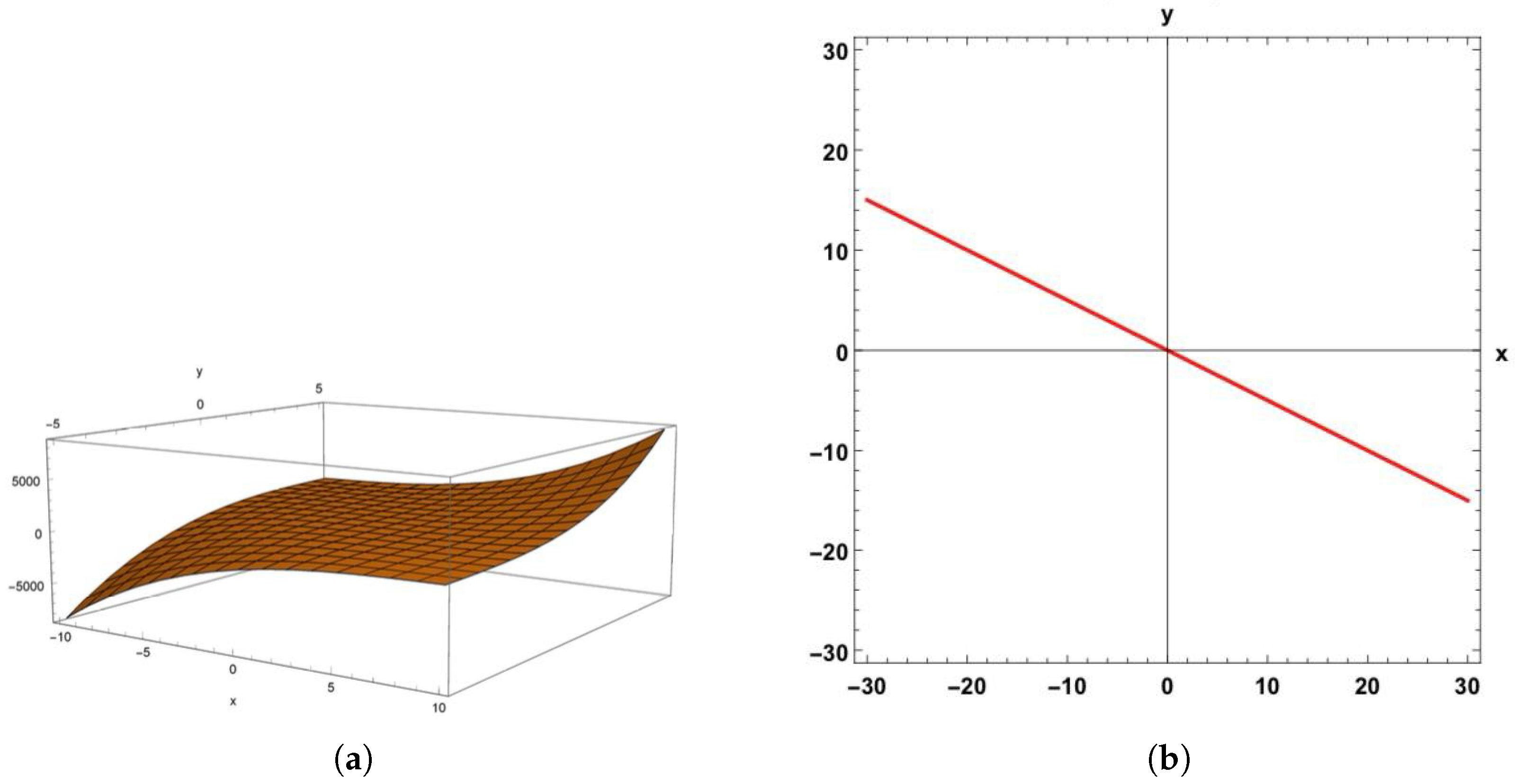
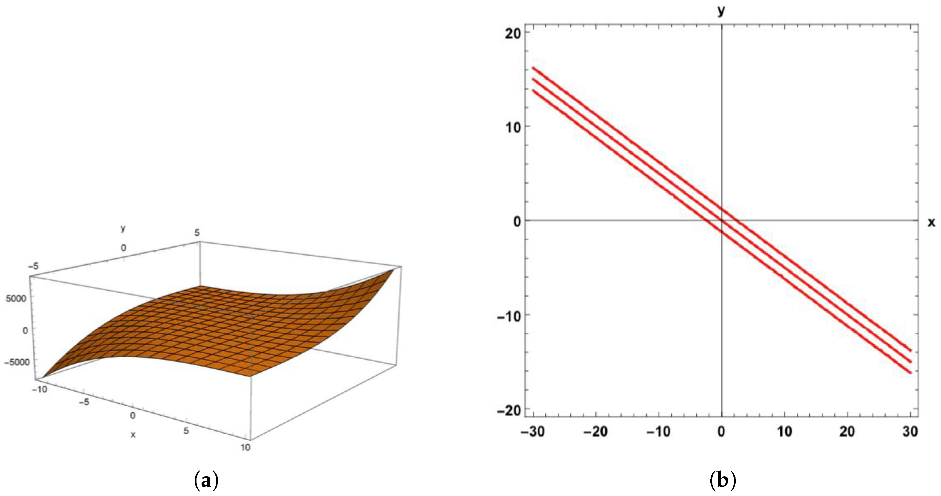
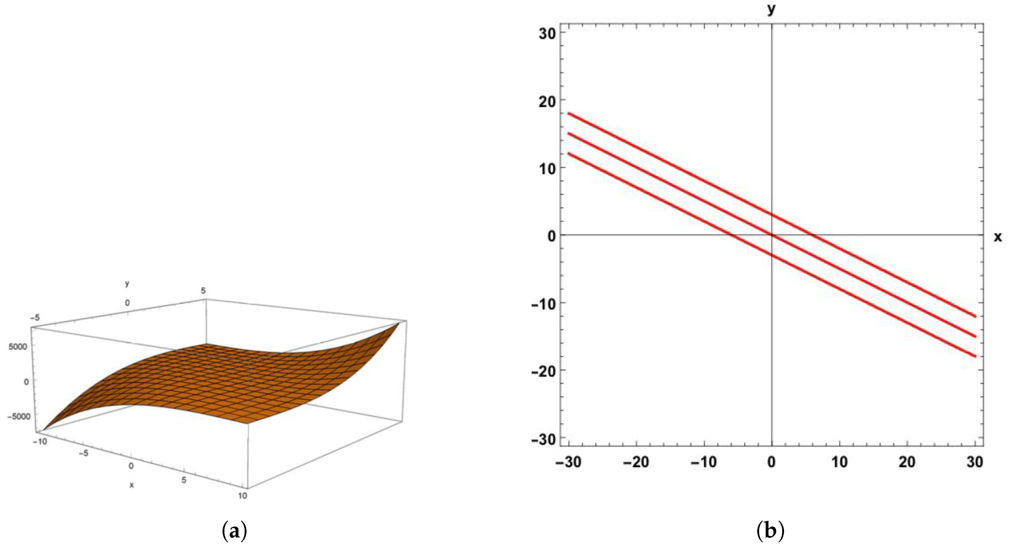
3.1. Truncated Exponential Based Hermite Type Polynomials

Let $\psi \left(y,t\right)=e^{2yt}$ and $A\left(t\right)=e^{-t^2}.$ The truncated-exponential-based Hermite-type polynomials can be defined via generating function as follows:

$$e^{xt+2yt-t^2}{\displaystyle \frac{1}{1-z{t}^m}}=\sum _{j=0}^{\infty }{\phantom{­}}_{e^{\left(m\right)}}{G}_j\left(x,y,z\right){\displaystyle \frac{t^j}{j!}}.$$

(40)

Corollary 1.

The polynomials ${\phantom{­}}_{e^{\left(m\right)}}{G}_j\left(x,y,z\right)$ have the following explicit representation

$$\begin{array}{c}\hfill {\phantom{­}}_{e^{\left(m\right)}}{G}_j\left(x,y,z\right)=\sum _{i=0}^j\sum _{l=0}^{\left[\frac{i}{m}\right]}\left({\displaystyle \genfrac{}{}{0pt}{}{j}{i}}\right)\left({\displaystyle \genfrac{}{}{0pt}{}{i}{ml}}\right)\left(ml\right)!x^{j-i}{z}^l{H}_{i-ml}\left(y\right)\end{array}$$

(41)

where $H_i\left(y\right)$ are Hermite polynomials [22] as follows

$$\begin{array}{c}\hfill \sum _{i=0}^{\infty }{H}_i\left(y\right){\displaystyle \frac{t^i}{i!}}=e^{2yt-t^2}.\end{array}$$

The first four truncated-exponential-based Hermite-type polynomials are as follows (

Table 1. The first four truncated-exponential-based Hermite-type polynomials.

j	${\phantom{­}}_{e^{\left(2\right)}}{G}_j\left(x,y,z\right)\left(m=2\right)$
0	1
1	$x+2y$
2	$x^2+4xy+4y^2+2z-2$
3	$x^3+8y^3+12yz+6xz+6x^{2}y+12x{y}^2-12y-6x.$

):

Corollary 2.

The truncated-exponential-based Hermite-type polynomials have the following determinant representation

$${\phantom{­}}_{e^{\left(m\right)}}{G}_j\left(x,y,z\right)={\left(-1\right)}^j\left|\begin{array}{ccccc}{G}_0^{\left(m\right)}\left(x,y,z\right)& G_1^{\left(m\right)}\left(x,y,z\right)& \dots & G_{j-1}^{\left(m\right)}\left(x,y,z\right)& G_j^{\left(m\right)}\left(x,y,z\right)\\ \\ 1& 0& \dots & {\gamma }_{j-1}& {\gamma }_j\\ \\ 0& 1& \dots & \left({\displaystyle \genfrac{}{}{0pt}{}{j-1}{1}}\right){\gamma }_{j-2}& \left({\displaystyle \genfrac{}{}{0pt}{}{j}{1}}\right){\gamma }_{j-1}\\ \\ 0& 0& \dots & \left({\displaystyle \genfrac{}{}{0pt}{}{j-1}{2}}\right){\gamma }_{j-3}& \left({\displaystyle \genfrac{}{}{0pt}{}{j}{2}}\right){\gamma }_{j-2}\\ \\ ⋮& ⋮& ⋮& ⋮& ⋮\\ \\ 0& 0& \dots & 1& \left({\displaystyle \genfrac{}{}{0pt}{}{j}{j-1}}\right){\gamma }_1\end{array}\right|$$

(42)

where ${\gamma }_0,{\gamma }_1,{\gamma }_2,\dots ,{\gamma }_j$ are the coefficients of the Maclaurin series of the function $e^{t^2}$ and

$$\sum _{j=0}^{\infty }{G}_j^{\left(m\right)}\left(x,y,z\right){\displaystyle \frac{t^j}{j!}}=e^{xt+2yt}{\displaystyle \frac{1}{1-z{t}^m}}.$$

Corollary 3.

The polynomials ${\phantom{­}}_{e^{\left(m\right)}}{G}_j\left(x,y,z\right)$ satisfy the following recurrence relation

$$\begin{array}{ccc}\hfill {\phantom{­}}_{e^{\left(m\right)}}{G}_{j+1}\left(x,y,z\right)& =& x{\phantom{­}}_{e^{\left(m\right)}}{G}_j\left(x,y,z\right)+zm\underset{i=0}{\sum ^{j-m+1}}{\displaystyle \frac{j!}{\left(j-i-m+1\right)!}}{e}_i^{\left(m\right)}\left(z\right){\phantom{­}}_{e^{\left(m\right)}}{G}_{j-i-m+1}\left(x,y,z\right)\hfill \\ & \phantom{­}& -2j{\phantom{­}}_{e^{\left(m\right)}}{G}_{j-1}\left(x,y,z\right)+2y{\phantom{­}}_{e^{\left(m\right)}}{G}_j\left(x,y,z\right),j\ge m-1\hfill \end{array}$$

where the polynomials $e_i^{\left(m\right)}\left(z\right)$ are defined in (29).

Corollary 4.

For the truncated-exponential-based Hermite-type polynomials ${\phantom{­}}_{e^{\left(m\right)}}{G}_j\left(x,y,z\right)$, we provide the following lowering operator ${\phantom{­}}_x{\varsigma }_j^{-},$ raising operator ${\phantom{­}}_x{\varsigma }_j^{+}$

$$\begin{array}{ccc}\hfill {\phantom{­}}_x{\varsigma }_j^{-}:& =& {\displaystyle \frac{1}{j}}{D}_x,\hfill \\ \hfill {\phantom{­}}_x{\varsigma }_j^{+}:& =& x+2y-2D_x+zm\underset{i=0}{\sum ^{j-m+1}}{e}_i^{\left(m\right)}\left(z\right)D_x^{i+m-1},j\ge m-1\hfill \end{array}$$

(43)

and differential equation

$$\left(\left(x+2y\right)D_x-2D_x^2+zm\underset{i=0}{\sum ^{j-m+1}}{e}_i^{\left(m\right)}\left(z\right)D_x^{i+m}-j\right){\phantom{­}}_{e^{\left(m\right)}}{G}_j\left(x,y,z\right)=0,j\ge m-1.$$

(44)

The $3D$ surface plot of the truncated-exponential-based Hermite-type polynomials ${\phantom{­}}_{e^{\left(2\right)}}{G}_j\left(x,y,z\right)$ and the distribution of real roots of zeros for the truncated-exponential-based Hermite-type polynomials ${\phantom{­}}_{e^{\left(2\right)}}{G}_j\left(x,y,z\right)$ are investigated for $j=3,m=2$. The surface plots of these polynomials and the distribution of real roots of zeros of them are given in Figure 1 for $j=3,m=2$ and $z=5$, in Figure 2 for $j=3,m=2$, and $z=0$ and in Figure 3 for $j=3,m=2$, and $z=-5$.

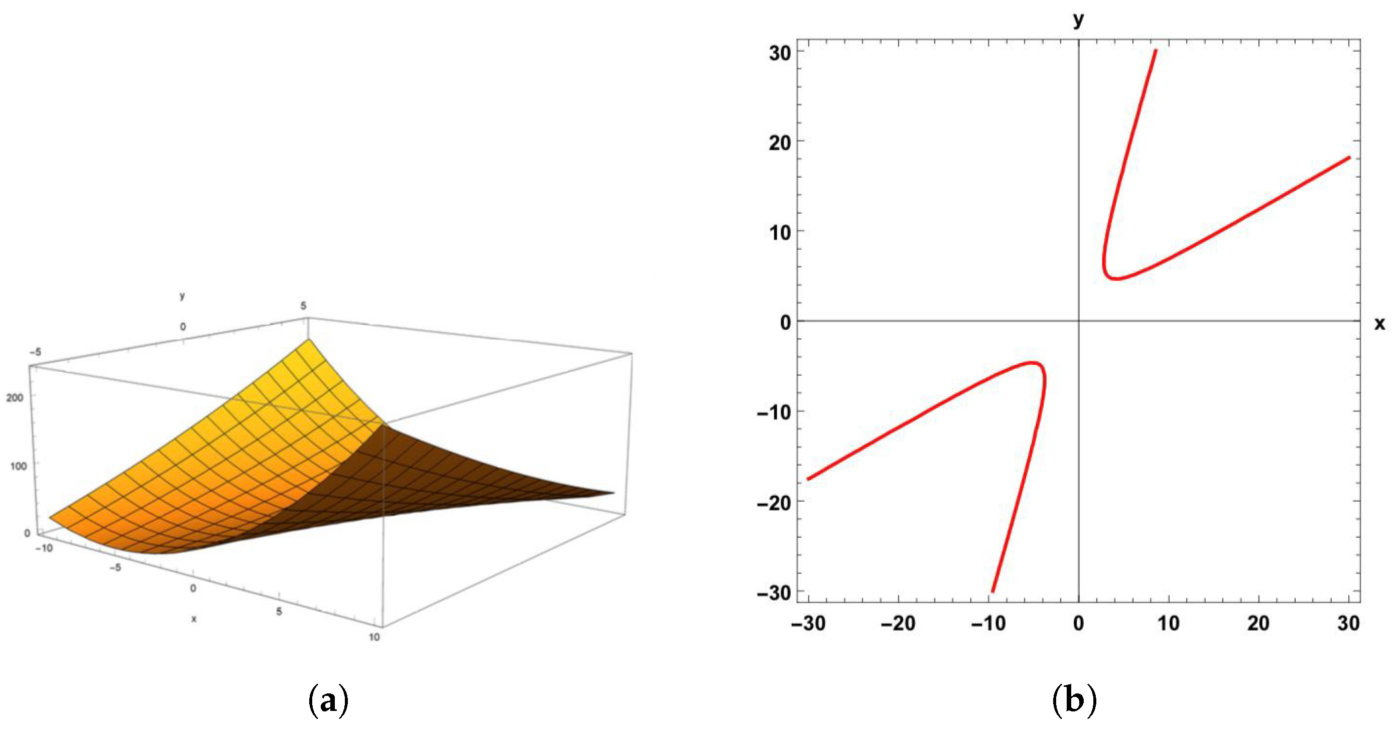
3.2. Truncated-Exponential-Based Laguerre–Frobenius Euler Polynomials

Let $\psi \left(y,t\right)=C_0\left(yt\right)$ and $A\left(t\right)={\displaystyle \frac{1-\mu }{e^t-\mu }}.$ The truncated-exponential-based Laguerre–Frobenius Euler polynomials can be defined with the help of generating function as follows:

$$\left({\displaystyle \frac{1-\mu }{e^t-\mu }}\right)e^{xt}{C}_0\left(yt\right){\displaystyle \frac{1}{1-z{t}^m}}=\sum _{j=0}^{\infty }{\phantom{­}}_{e^{\left(m\right)}}{L}_j^F\left(x,y,z;\mu \right){\displaystyle \frac{t^j}{j!}},\left(\mu \ne 1\right)$$

(45)

where $C_0\left(y\right)$ denotes the 0-th order Tricomi function. The j-th order Tricomi functions $C_j\left(y\right)$ [23] are defined as

$$\begin{array}{c}\hfill C_j\left(y\right)=\sum _{i=0}^{\infty }{\displaystyle \frac{{\left(-1\right)}^i{y}^i}{i!\left(j+i\right)!}}.\end{array}$$

(46)

Corollary 5.

The polynomials ${\phantom{­}}_{e^{\left(m\right)}}{L}_j^F\left(x,y,z;\mu \right)$ have the following explicit representation

$$\begin{array}{c}\hfill {\phantom{­}}_{e^{\left(m\right)}}{L}_j^F\left(x,y,z;\mu \right)=\sum _{i=0}^j\sum _{r=0}^{\left[\frac{i}{m}\right]}\left({\displaystyle \genfrac{}{}{0pt}{}{j}{i}}\right)\left({\displaystyle \genfrac{}{}{0pt}{}{i}{mr}}\right)\left(mr\right)!z^r{L}_{i-mr}\left(x,y\right)E_{j-i}^F\left(\mu \right)\end{array}$$

(47)

where the polynomials $L_i\left(x,y\right)$ are two-variable Laguerre polynomials [23] and the numbers $E_i^F\left(\mu \right)$ are Frobenius–Euler numbers [24] as follows:

$$\begin{array}{ccc}\hfill \sum _{i=0}^{\infty }{L}_i\left(x,y\right){\displaystyle \frac{t^i}{i!}}& =& e^{xt}{C}_0\left(yt\right),\hfill \\ \hfill \sum _{i=0}^{\infty }{E}_i^F\left(\mu \right){\displaystyle \frac{t^i}{i!}}& =& {\displaystyle \frac{1-\mu }{e^t-\mu }},\hfill \end{array}$$

respectively.

The first four truncated-exponential-based Laguerre–Frobenius Euler polynomials are as follows (

Table 2. The first four truncated-exponential-based Laguerre–Frobenius Euler polynomials.

j	${\phantom{­}}_{e^{\left(2\right)}}{L}_j^F\left(x,y,z;\mu \right)\left(m=2\right)$
0	1
1	$x+{\displaystyle \frac{1}{\mu -1}}-y$
2	${\displaystyle \frac{2z}{{\left(\mu -1\right)}^2}}-2{\displaystyle \frac{x}{{\left(\mu -1\right)}^2}}+{\displaystyle \frac{\mu }{{\left(\mu -1\right)}^2}}+{\displaystyle \frac{{\mu }^2{x}^2}{{\left(\mu -1\right)}^2}}+{\displaystyle \frac{2x\mu }{{\left(\mu -1\right)}^2}}-{\displaystyle \frac{4z\mu }{{\left(\mu -1\right)}^2}}$
	$-{\displaystyle \frac{2x^2\mu }{{\left(\mu -1\right)}^2}}+{\displaystyle \frac{2z{\mu }^2}{{\left(\mu -1\right)}^2}}+{\displaystyle \frac{x^2}{{\left(\mu -1\right)}^2}}+{\displaystyle \frac{1}{{\left(\mu -1\right)}^2}}-2y\left(x+{\displaystyle \frac{1}{\mu -1}}\right)+{\displaystyle \frac{y^2}{2}}$
3	${\displaystyle \frac{1}{{\left(\mu -1\right)}^3}}\left(-x^3+x^3{\mu }^3-3x^3{\mu }^2+3x^3\mu +3x^2+3x^2{\mu }^2-6x^2\mu -3x+3x{\mu }^2+18xz\mu \right)$
	${\displaystyle \frac{1}{{\left(\mu -1\right)}^3}}\left(-18xz{\mu }^2-6xz+6xz{\mu }^3+6z-12z\mu +6z{\mu }^2+4\mu +{\mu }^2+1\right)$
	$-{\displaystyle \frac{3y}{{\left(\mu -1\right)}^2}}\left(2z-2x+\mu +x^2{\mu }^2+2x\mu -4z\mu -2x^2\mu +2z{\mu }^2+x^2+1\right)+{\displaystyle \frac{3}{2}}{y}^2\left(x+{\displaystyle \frac{1}{\mu -1}}\right)-{\displaystyle \frac{1}{6}}{y}^3.$

):

Corollary 6.

The truncated-exponential-based Laguerre–Frobenius Euler polynomials have the following determinant representation

$${\phantom{­}}_{e^{\left(m\right)}}{L}_j^F\left(x,y,z;\mu \right)={\left(-1\right)}^j\left|\begin{array}{ccccc}{L}_0^{\left(m\right)}\left(x,y,z\right)& L_1^{\left(m\right)}\left(x,y,z\right)& \dots & L_{j-1}^{\left(m\right)}\left(x,y,z\right)& L_j^{\left(m\right)}\left(x,y,z\right)\\ \\ 1& {\displaystyle \frac{1}{1-\mu }}& \dots & {\displaystyle \frac{1}{1-\mu }}& {\displaystyle \frac{1}{1-\mu }}\\ \\ 0& 1& \dots & \left({\displaystyle \genfrac{}{}{0pt}{}{j-1}{1}}\right){\displaystyle \frac{1}{1-\mu }}& \left({\displaystyle \genfrac{}{}{0pt}{}{j}{1}}\right){\displaystyle \frac{1}{1-\mu }}\\ \\ 0& 0& \dots & \left({\displaystyle \genfrac{}{}{0pt}{}{j-1}{2}}\right){\displaystyle \frac{1}{1-\mu }}& \left({\displaystyle \genfrac{}{}{0pt}{}{j}{2}}\right){\displaystyle \frac{1}{1-\mu }}\\ \\ ⋮& ⋮& ⋮& ⋮& ⋮\\ \\ 0& 0& \dots & 1& \left({\displaystyle \genfrac{}{}{0pt}{}{j}{j-1}}\right){\displaystyle \frac{1}{1-\mu }}\end{array}\right|$$

(48)

where

$$\sum _{j=0}^{\infty }{L}_j^{\left(m\right)}\left(x,y,z;\mu \right){\displaystyle \frac{t^j}{j!}}=e^{xt}{C}_0\left(yt\right){\displaystyle \frac{1}{1-z{t}^m}}.$$

Corollary 7.

The recurrence relation satisfied by truncated-exponential-based Laguerre–Frobenius Euler polynomials ${\phantom{­}}_{e^{\left(m\right)}}{L}_j^F\left(x,y,z;\mu \right)$ is given by

$$\begin{array}{ccc}\hfill {\phantom{­}}_{e^{\left(m\right)}}{L}_{j+1}^F\left(x,y,z;\mu \right)& =& x{\phantom{­}}_{e^{\left(m\right)}}{L}_j^F\left(x,y,z;\mu \right)-D_y^{-1}{\phantom{­}}_{e^{\left(m\right)}}{L}_j^F\left(x,y,z;\mu \right)\hfill \\ & \phantom{­}& +zm\underset{i=0}{\sum ^{j-m+1}}{\displaystyle \frac{j!}{\left(j-i-m+1\right)!}}{e}_i^{\left(m\right)}\left(z\right){\phantom{­}}_{e^{\left(m\right)}}{L}_{j-i-m+1}^F\left(x,y,z;\mu \right)\hfill \\ & \phantom{­}& +{\displaystyle \frac{1}{1-\mu }}\sum _{i=0}^j\left({\displaystyle \genfrac{}{}{0pt}{}{j}{i}}\right){\mathcal{E}}_{j-i}^F\left(\mu \right){\phantom{­}}_{e^{\left(m\right)}}{L}_i^F\left(x,y,z;\mu \right),j\ge m-1\hfill \end{array}$$

where ${\mathcal{E}}_i^F\left(\mu \right)$ are related by the Frobenius–Euler polynomials $E_i^F\left(x;\mu \right)$ [25] as follows:

$${\mathcal{E}}_i^F\left(\mu \right):=-\sum _{l=0}^i\left({\displaystyle \genfrac{}{}{0pt}{}{i}{l}}\right){\displaystyle \frac{1}{2^l}}{E}_{i-l}^F\left({\displaystyle \frac{1}{2}};\mu \right)$$

and the polynomials $e_i^{\left(m\right)}\left(z\right)$ are defined in (29) and $D_y^{-1}$ inverse of $D_y:={\displaystyle \frac{\partial }{\partial y}}$.

Corollary 8.

For the truncated-exponential-based Laguerre–Frobenius Euler polynomials ${\phantom{­}}_{e^{\left(m\right)}}{L}_j^F\left(x,y,z;\mu \right)$, we give the following lowering operator ${\phantom{­}}_x{\varsigma }_j^{-},$ raising operator ${\phantom{­}}_x{\varsigma }_j^{+}$

$$\begin{array}{ccc}\hfill {\phantom{­}}_x{\varsigma }_j^{-}:& =& {\displaystyle \frac{1}{j}}{D}_x,\hfill \\ \hfill {\phantom{­}}_x{\varsigma }_j^{+}:& =& x-D_y^{-1}+zm\underset{i=0}{\sum ^{j-m+1}}{e}_i^{\left(m\right)}\left(z\right)D_x^{i+m-1}+{\displaystyle \frac{1}{1-\mu }}\sum _{i=0}^j{\displaystyle \frac{{\mathcal{E}}_{j-i}^F\left(\mu \right)}{\left(j-i\right)!}}{D}_x^{j-i},j\ge m-1,\hfill \end{array}$$

(49)

and differential equation

$$\left(x{D}_x-D_y^{-1}{D}_x+zm\underset{i=0}{\sum ^{j-m+1}}{e}_i^{\left(m\right)}\left(z\right)D_x^{i+m}+{\displaystyle \frac{1}{1-\mu }}\sum _{i=0}^j{\displaystyle \frac{{\mathcal{E}}_{j-i}^F\left(\mu \right)}{\left(j-i\right)!}}{D}_x^{j-i+1}-j\right){\phantom{­}}_{e^{\left(m\right)}}{L}_j^F\left(x,y,z;\mu \right)=0,j\ge m-1,$$

(50)

respectively.

The $3D$ surface plot of truncated-exponential-based Laguerre–Frobenius Euler polynomials ${\phantom{­}}_{e^{\left(2\right)}}{L}_j^F\left(x,y,z;\mu \right)$ and the distribution of real roots of zeros for truncated-exponential-based Laguerre–Frobenius Euler polynomials ${\phantom{­}}_{e^{\left(2\right)}}{L}_j^F\left(x,y,z;\mu \right)$ are investigated for $j=m=2$. The surface plots of these polynomials and the distribution of real roots of zeros of them are given in Figure 4 for $j=m=2,\mu =3$ and $z=5$, in Figure 5 for $j=m=2,\mu =3$ and $z=0$ and in Figure 6 for $j=m=2,\mu =3$ and $z=-5$.

4. Conclusions

In this research paper, we define truncated-exponential-based general-Appell polynomials with the help of general-Appell polynomials and truncated-exponential-based Appell polynomials. Then, we give the explicit representation and determinant representation of these polynomials. We derive the recurrence relation, lowering and raising operators, and differential equation. Also, we study new families of truncated-exponential-based subpolynomials by examining special cases. Special cases of this family such as truncated-exponential-based Hermite-type and truncated-exponential-based Laguerre–Frobenius Euler polynomials are studied and their corresponding properties are obtained.

On the other hand, it is known that Bell polynomials, another important class of polynomials involving the exponential function, have been used to study soliton equations and their bilinear formalizations [26,27]. Moreover, a class of resonant solutions has been characterized through the use of Bell polynomials [28]. One can define the truncated-exponential-based Bell polynomials as a special case of our main polynomial family and it is not hard to predict that these polynomials will have potential applications in many areas such as soliton theory. This will be a new topic of discussion and an open question for future studies.

References

1. Dattoli, G.; Cesarano, C.; Sacchetti, D. A note on truncated polynomials. Appl. Math. Comput. 2003, 134, 595–605. [Google Scholar] [CrossRef]
2. Srivastava, H.M.; Araci, S.; Khan, W.A.; Acikgoz, M. A note on the truncated-exponential based Apostol-type polynomials. Symmetry 2019, 11, 538. [Google Scholar] [CrossRef]
3. Duran, U.; Açıkgöz, M. Truncated Fubini polynomials. Mathematics 2019, 7, 431. [Google Scholar] [CrossRef]
4. Duran, U.; Açıkgöz, M. On degenerate truncated special polynomials. Mathematics 2020, 8, 144. [Google Scholar] [CrossRef]
5. Kumam, W.; Srivastava, H.M.; Wani, S.A.; Araci, S.; Kumam, P. Truncated-exponential-based Frobenius–Euler polynomials. Adv. Differ. Equ. 2019, 2019, 530. [Google Scholar] [CrossRef]
6. Raza, N.; Fadel, M.; Cesarano, C. A note on q-truncated exponential polynomials. Carpathian Math. Publ. 2024, 16, 128–147. [Google Scholar] [CrossRef]
7. Costabile, F.A.; Khan, S.; Ali, H. A study of the q-truncated exponential–Appell polynomials. Mathematics 2024, 12, 3862. [Google Scholar] [CrossRef]
8. Andrews, L.C. Special Functions for Engineers and Applied Mathematicians; Macmillan: New York, NY, USA, 1985. [Google Scholar]
9. Dattoli, G.; Migliorati, M.; Srivastava, H.M. A class of Bessel summation formulas and associated operational methods. Fract. Calc. Appl. Anal. 2004, 7, 169–176. [Google Scholar]
10. Roman, S. The Umbral Calculus; Academic Press Inc.: New York, NY, USA, 1984. [Google Scholar]
11. Sheffer, I.M. Note on Appell polynomials. Bull. Am. Math. Soc. 1945, 51, 739–744. [Google Scholar] [CrossRef]
12. Khan, S.; Raza, N. General-Appell polynomials within the context of monomiality principle. Int. J. Anal. 2013, 2013, 328032. [Google Scholar] [CrossRef]
13. Khan, S.; Yasmin, G.; Khan, R.; Hassan, N.A.M. Hermite-based Appell polynomials: Properties and applications. J. Math. Anal. Appl. 2009, 351, 756–764. [Google Scholar] [CrossRef]
14. Khan, S.; Al-Saad, M.W.; Khan, R. Laguerre-based Appell polynomials: Properties and applications. Math. Comput. Model. 2010, 52, 247–259. [Google Scholar] [CrossRef]
15. Zayed, M.; Wani, S.A.; Subzar, M.; Riyasat, M. Certain families of differential equations associated with the generalized 1-parameter Hermite–Frobenius Euler polynomials. Math. Comput. Model. Dyn. Syst. 2024, 30, 683–700. [Google Scholar] [CrossRef]
16. Costabile, F.A.; Longo, E. A determinantal approach to Appell polynomials. J. Comput. Appl. Math. 2010, 234, 1528–1542. [Google Scholar] [CrossRef]
17. Yang, Y. Determinant representations of Appell polynomial sequences. Oper. Matrices 2008, 2, 517–524. [Google Scholar] [CrossRef]
18. Costabile, F. Modern Umbral Calculus: An Elementary Introduction with Applications to Linear Interpolation and Operator Approximation Theory; Walter de Gruyter GmbH Co. KG: Berlin, Germany, 2019; Volume 72. [Google Scholar]
19. Costabile, F.A.; Gualtieri, M.I.; Napoli, A. Polynomial Sequences: Basic Methods, Special Classes, and Computational Applications; Walter de Gruyter GmbH, Co. KG: Berlin, Germany, 2023. [Google Scholar]
20. Costabile, F.A.; Gualtieri, M.I.; Napoli, A. Bivariate general Appell interpolation problem. Numer. Algorithms 2022, 91, 531–556. [Google Scholar] [CrossRef]
21. Khan, S.; Yasmin, G.; Ahmad, N. A note on truncated exponential-based Appell polynomials. Bull. Malays. Math. Sci. Soc. 2017, 40, 373–388. [Google Scholar] [CrossRef]
22. Dattoli, G.; Chiccoli, C.; Lorenzutta, S.; Maino, G.; Torre, A. Theory of generalized Hermite polynomials. Comput. Math. Appl. 1994, 28, 71–83. [Google Scholar] [CrossRef]
23. Dattoli, G.; Torre, A.; Mancho, A.M. The generalized Laguerre polynomials, the associated Bessel functions and application to propagation problems. Radiat. Phys. Chem. 2000, 59, 229–237. [Google Scholar] [CrossRef]
24. Carlitz, L. Eulerian numbers and polynomials. Math. Mag. 1959, 32, 247–260. [Google Scholar] [CrossRef]
25. Araci, S.; Riyasat, M.; Wani, S.A.; Khan, S. Differential and integral equations for the 3-variable Hermite-Frobenius-Euler and Frobenius-Genocchi polynomials. Appl. Math. Inf. Sci. 2017, 11, 1335–1346. [Google Scholar] [CrossRef]
26. Ma, W.X. Bilinear equations, Bell polynomials and linear superposition principle. J. Phys. Conf. Ser. 2013, 411, 012021. [Google Scholar] [CrossRef]
27. Ma, W.X. Trilinear equations, Bell polynomials, and resonant solutions. Front. Math. China 2013, 8, 1139–1156. [Google Scholar] [CrossRef]
28. Ma, W.X. Bilinear equations and resonant solutions characterized by Bell polynomials. Rep. Math. Phys. 2013, 72, 41–56. [Google Scholar] [CrossRef]
Figure 1. The polynomials ­ e 2 G 3 x , y , 5 . (a) Surface plot of ­ e 2 G 3 x , y , 5 . (b) Distribution of real roots of zeros of ­ e 2 G 3 x , y , 5 .
Mathematics 13 01266 g001
Figure 2. The polynomials ­ e 2 G 3 x , y , 0 . (a) Surface plot of ­ e 2 G 3 x , y , 0 . (b) Distribution of real roots of zeros of ­ e 2 G 3 x , y , 0 .
Mathematics 13 01266 g002
Figure 3. The polynomials ­ e 2 G 3 x , y , 5 . (a) Surface plot of ­ e 2 G 3 x , y , 5 . (b) Distribution of real roots of zeros of ­ e 2 G 3 x , y , 5 .
Mathematics 13 01266 g003
Figure 4. The polynomials ­ e 2 L 2 F x , y , 5 ; 3 . (a) Surface plot of ­ e 2 L 2 F x , y , 5 ; 3 . (b) Distribution of real roots of zeros of ­ e 2 L 2 F x , y , 5 ; 3 .
Mathematics 13 01266 g004
Figure 5. The polynomials ­ e 2 L 2 F x , y , 0 ; 3 . (a) Surface plot of ­ e 2 L 2 F x , y , 0 ; 3 . (b) Distribution of real roots of zeros of ­ e 2 L 2 F x , y , 0 ; 3 .
Mathematics 13 01266 g005
Figure 6. The polynomials ­ e 2 L 2 F x , y , 5 ; 3 . (a) Surface plot of ­ e 2 L 2 F x , y , 5 ; 3 . (b) Distribution of real roots of zeros of ­ e 2 L 2 F x , y , 5 ; 3 .
Mathematics 13 01266 g006