Article

Predictive Maintenance for Cutter System of Roller Laminator

1
Department of Industrial Engineering and Management, Ming Chi University of Technology, New Taipei City 243303, Taiwan
2
Center for Artificial Intelligence & Data Science, Ming Chi University of Technology, New Taipei City 243303, Taiwan
3
Manufacturing Engineering and Management Department, De La Salle University, Manila 0922, Philippines
4
Center for Engineering and Sustainable Development Research, De La Salle University, Manila 0922, Philippines
5
Metal Industries Research & Development Centre, Kaohsiung City 811, Taiwan
6
Department of Foreign Languages and Literature, National Ilan University, Ilan 260007, Taiwan
*
Authors to whom correspondence should be addressed.
Mathematics 2025, 13(8), 1264; https://doi.org/10.3390/math13081264
Submission received: 5 March 2025 / Revised: 26 March 2025 / Accepted: 8 April 2025 / Published: 11 April 2025
(This article belongs to the Special Issue Applied Statistics in Management Sciences)

Abstract

:
In the era of Industry 4.0, equipment maintenance is shifting toward data-driven strategies. Traditional methods rely on usage time or cycle counts to estimate component lifespan. This often causes early replacement of parts, leading to increased production costs. This study focuses on the cutter system of a roller laminator used in printed circuit board (PCB) manufacturing. An accelerometer is used to collect vibration signals under normal and abnormal states. Fast Fourier transform (FFT) is used to convert time-domain data into the frequency domain, then key statistical features from critical frequency bands are extracted as independent variables. The study applies logistic regression (LR), random forest (RF), and support vector machine (SVM) for predictive modeling of the cutting tool’s condition. The results show that the prediction accuracies of these models are 87.55%, 93.77%, and 94.94%, respectively, with SVM performing the best.

1. Introduction

The printed circuit board (PCB) industry has undergone significant transformations, evolving from early bulky and outdated designs to modern high-density interconnect PCBs (HDI PCBs) and integrated circuit (IC) substrates. These advanced boards incorporate fine-line technology, enhancing circuit density and performance. However, as manufacturing technology advances and the demand for intelligent production increases, reducing the scrap rate has become a critical challenge for the industry.
The multi-layer PCB manufacturing process includes several key stages. It starts with substrate preparation, followed by inner and outer layer processing, where dry film lamination, ultraviolet radiation (UV) exposure, developing, and etching form circuit patterns. Lamination, drilling, and copper plating integrate multiple layers and establish electrical connections. A solder mask prevents short circuits, while surface finishing improves conductivity and corrosion resistance. Finally, inspection and profiling ensure quality through cutting, edge finishing, and electrical testing.
A roller laminator is commonly used in both the inner and outer layer processes of multi-layer PCB fabrication for dry film lamination. Its primary function is to press the dry film photoresist (DFP) onto the copper-clad laminate (CCL). As shown in Figure 1, the process begins with aligning the copper-clad laminate to ensure precise positioning. As the laminate enters the lamination zone, the film alignment mechanism pulls the dry film to the leading edge of the board. The heated roller then presses the dry film onto the copper surface. Once the lamination is complete, a cutter automatically trims the film, and the laminated board is transferred to the exposure process.
Maintaining the condition of cutter blades directly affects product quality and production efficiency. Initially, factories made the maintenance strategy run-to-failure (R2F) [1]. This method came from the era of Industry 1.0 and 2.0 which involved repairing equipment only after a failure occurred. Although simple, it often led to production interruptions and high repair costs. Then, factories monitored component lifespans based on usage time or cycle counts. This preventive maintenance (PvM) strategy, popularized during the Industry 3.0 era of digital control and automation, sought to reduce failures by performing scheduled maintenance. However, this time-based approach often fails to capture real-time equipment conditions. In practice, components may still fail earlier than expected due to equipment malfunctions, process variations, or human errors.
With the rise in smart manufacturing and Industry 4.0, enterprises are adopting the internet of things (IoT) and smart sensors to enable predictive maintenance (PdM) through real-time data collection and artificial intelligence (AI) analysis. A data-driven approach not only enhances equipment availability but also optimizes maintenance strategies, reducing production losses caused by unexpected failures. This study focuses on intelligent monitoring of roller laminator cutters. By leveraging sensing technology and machine learning techniques, it aims to achieve real-time health diagnostics and provide optimal replacement recommendations.
Romanssini et al. [2] mentioned that vibration signal processing techniques can monitor rotating machinery, identify defects, or detect feature variations. Common techniques include time-domain analysis and frequency domain analysis. This study employs an accelerometer to collect voltage signals of vibrations under both normal and abnormal conditions. The collected time-domain signals are then transformed into the frequency domain using fast Fourier transform (FFT) for signal analysis and noise filtering. Critical statistical features are extracted from the spectrum to distinguish between normal and abnormal states. In the systematic study on machine learning-based predictive maintenance, Carvalho et al. [3] defined a structured modeling framework comprising historical data selection, data preprocessing, model selection, training and validation, and model maintenance. Based on this framework, we subsequently constructed multiple machine learning classifiers to evaluate and compare predictive performance.
To the best of our knowledge, the PdM application to cutter system of roller laminators in PCB manufacturing remains scarce. The first contributions of this study lie in bridging a gap between PdM techniques and their application in a specific and underexplored industrial component. The second contribution is the development of a vibration signal acquisition and transmission system deployed in a real industrial environment. The system enables end-to-end data collection through strategically placed accelerometer sensors, with automated data transmission facilitated by programmable logic controller (PLC) signals and Ethernet control automation technology (EtherCAT). This implementation showcases not only the academic relevance but also the practical feasibility of the proposed approach for deployment in smart manufacturing settings. The third contribution is the development of a customized three-stage frequency-domain feature extraction pipeline that extends beyond conventional FFT analysis. By integrating amplitude difference analysis, energy ratio evaluation, k-means clustering for frequency band identification, and frequency statistic extraction, the proposed method identifies physically meaningful vibration patterns associated with cutter wear. This structured feature engineering process enhances both the interpretability and the effectiveness of the monitoring system.
The remainder of this paper is structured as follows: Section 2 reviews related research, covering topics such as machinery health monitoring and applications of machine learning in vibration signal analysis. Section 3 describes data collection, feature extraction, machine learning modeling, and evaluation methods. Section 4 presents model training and testing procedures along with result analysis. Section 5 summarizes the research findings and discusses potential future developments.

2. Applications of Machine Learning in PdM

Several studies have explored the integration of data preprocessing techniques with machine learning models for PdM, as summarized in Table 1. These studies demonstrate effective classification and anomaly prediction across various equipment and electromechanical components. The findings contribute to the development of a suitable research framework for this study.
Cerrada et al. [4] investigated PdM in gearboxes by extracting vibration signal features using time-domain statistical analysis, FFT, and wavelet packet transform (WPT). They classified seven different gear damage levels and applied genetic algorithms (GA) for feature selection with a random forest (RF) model. Their results showed that combining time-domain and frequency-domain statistical features achieved a precision of 94.66%, WPT-based RF reached 96.95%, and incorporating all three feature types with GA optimization improved precision to 97.81%. Madhusudana et al. [5] focused on face milling tools by extracting features from acoustic signals using discrete wavelet transform (DWT). They classified four tool conditions—new, worn, damaged, and chipped—by extracting features from 50 audio signals per condition. Different feature extraction methods, including statistical features, empirical mode decomposition (EMD), and DWT, were compared. Decision tree (DT) was used for feature selection, and four machine learning models, including support vector machine (SVM), multilayer perceptron (MLP), naïve Bayes (NB), and K-Star, were tested. Results indicated that DWT-based feature extraction had the highest accuracy, with DWT-DT-SVM achieving 83%, MLP 80%, NB 78.5%, and K-Star 76.5%. Kanawaday et al. [6] studied packaging film-slitting machines by extracting features such as time, tension, pressure, width, and diameter, using the difference method (DM). They classified machine states as normal or faulty using the autoregressive integrated moving average (ARIMA) model to predict production parameters, followed by classification using four supervised models. The results showed that deep neural network (DNN) had the highest accuracy at 98.69%, followed by NB (96.61%), SVM (95.52%), and classification and regression tree (CART) (94.46%). Madhusudana et al. [7] focused on face milling tools by extracting vibration signal features using DWT. They classified tool states into normal, side wear, chipping, and fracture faults. DT was used for feature selection, and classification results were compared between different kernel functions in SVM models, C-SVC and V-SVC. Results showed that C-SVC and V-SVC achieved 94.5% and 94% accuracy, respectively. Bonci et al. [8] examined belt drive systems by extracting current signal features using DWT. They assessed the impact of belt looseness on current signals and identified different belt tension levels. Results showed that looser belts raised signal energy and led to unhealthy and scattered signals. Sikder et al. [9] investigated motor bearings by extracting FFT-based features from vibration signals under normal and three faulty conditions. They applied data normalization and RF classification. Results showed that adjusting the RF estimator count to 400 achieved an optimal accuracy of 98.97%. Esakimuthu et al. [10] analyzed bearing faults using FFT-based current signal features. They examined normal bearings, and two defective conditions include outer ring holes and surface scratches. Machine learning and deep learning models were compared. With 320 training samples, SVM and k-nearest neighbors (KNN) achieved 81.96% and 86.25% accuracy, respectively, while convolutional neural network (CNN) reached 82.7%. When the sample size increased to 640, accuracy improved to 83.04% for SVM, 87.85% for KNN, and 89.26% for CNN. Results suggest that machine learning performs well with smaller datasets, while deep learning benefits from larger datasets. Ali et al. [11] applied PdM to induction motors by extracting current and vibration signal features using WPT. They analyzed six mechanical and six electrical fault types. Machine learning models, including SVM and KNN, achieved 100% accuracy when combining current and vibration signals. Magadán et al. [12] examined pumps in a dairy plant sterilization line by installing vibration sensors. They collected data from pumps with different maintenance cycles and used FFT to convert time-domain data into frequency-domain features. Results showed distinct waveform patterns at 25 Hz, 100 Hz, and 300 Hz for pump 1, and at 25 Hz and 200 Hz for pump 2, demonstrating the effectiveness of frequency-domain analysis. Saberi et al. [13] investigated eccentricity faults in induction motors by extracting FFT-based current and vibration signal features. They classified motor conditions into normal and six types of eccentricity-related faults. Using RF for feature selection and SVM for classification, they achieved an accuracy of 97.86%. Pollak et al. [14] studied belt drive systems by extracting FFT-based vibration signal features. They classified system conditions into normal and damaged states using an autoencoder model. The horizontal sensor setup achieved an F1 score of 98.89%, while the vertical setup reached 99.33%, both providing excellent fault detection. Xiang et al. [15] analyzed motor bearings by extracting FFT-based features and classified them into normal and nine different fault types. Using eXtreme gradient boosting (XGBoost) for classification, they achieved an accuracy of 98.12%. Giri et al. [16] investigated stator winding faults by extracting FFT-based current and axial flux features. They classified motor states into normal and six fault types related to high-impedance and low-impedance conditions. They used power spectral density (PSD) and six machine learning models. RF achieved the highest accuracy at 100%, followed by DT (96.77%), gradient boosting (90.32%), NB (90.32%), KNN (87.1%), and SVM (80.6%). Raouf et al. [17] analyzed six-axis robotic arms by extracting waveform, statistical, and kinetic features from current signals. They classified robotic arm conditions into normal, faulty, and aging states. They applied correlation analysis and Chi-square tests for feature selection. The accuracy of NB, SVM, KNN, and ensemble subspace classification was 96.7%, 96.1%, 86.1%, and 82.2%, respectively. Hosseinpour-Zarnaq et al. [18] studied tractor gearboxes using DWT-based vibration features. They classified gear conditions into normal and three types of tooth defects, including missing teeth, chipped teeth, and worn teeth. They compared results with and without correlation-based feature selection (CFS). Without CFS, RF and MLP achieved 86.25% and 82.5% accuracy, respectively. With CFS, accuracy improved to 92.5% and 86.25%, showing that RF outperformed MLP with limited data. Aburakhia et al. [19] analyzed bearings by extracting FFT, short-time Fourier transform (STFT), and WPT features using similarity-based PdM (SB-PdM) V1.0 software. They classified bearing conditions into normal and nine different fault types. They compared structure similarity, cosine similarity, and Euclidean distance. Results showed that using FFT-based cosine similarity achieved the highest accuracy at 99.6%. Souza et al. [20] focused on hydraulic turbines, analyzing cavitation and normal operating conditions using FFT-based vibration features. They classified turbine states and found that the MLP achieved 100% accuracy, while the radial basis function neural network (RBFNN) reached 95.29%. Hakami [21] proposed a PdM method using generative adversarial networks (GANs) to generate synthetic failure data, long short-term memory (LSTM) to extract temporal features, and failure horizons to address data imbalance. The models detected the status of non-woven materials machinery and predicted remaining useful life using time-series sensor data like vibration and temperature. Among classifiers, MLP achieved the best accuracy at 88.98%. Khalil and Rostam [22] presented a PdM method for rotating machinery, focusing on fault detection using vibration signals. The system extracted energy features from FFT, then classified machine conditions as normal, unbalanced, bearing defect, or combined faults. The best performance was achieved using a stacking ensemble of SVM and MLP, reaching 93.1% accuracy.
The objective of this study is to develop a method for classifying anomalies in the cutter system of a roller laminating machine. Based on the literature review, the following insights have been derived:
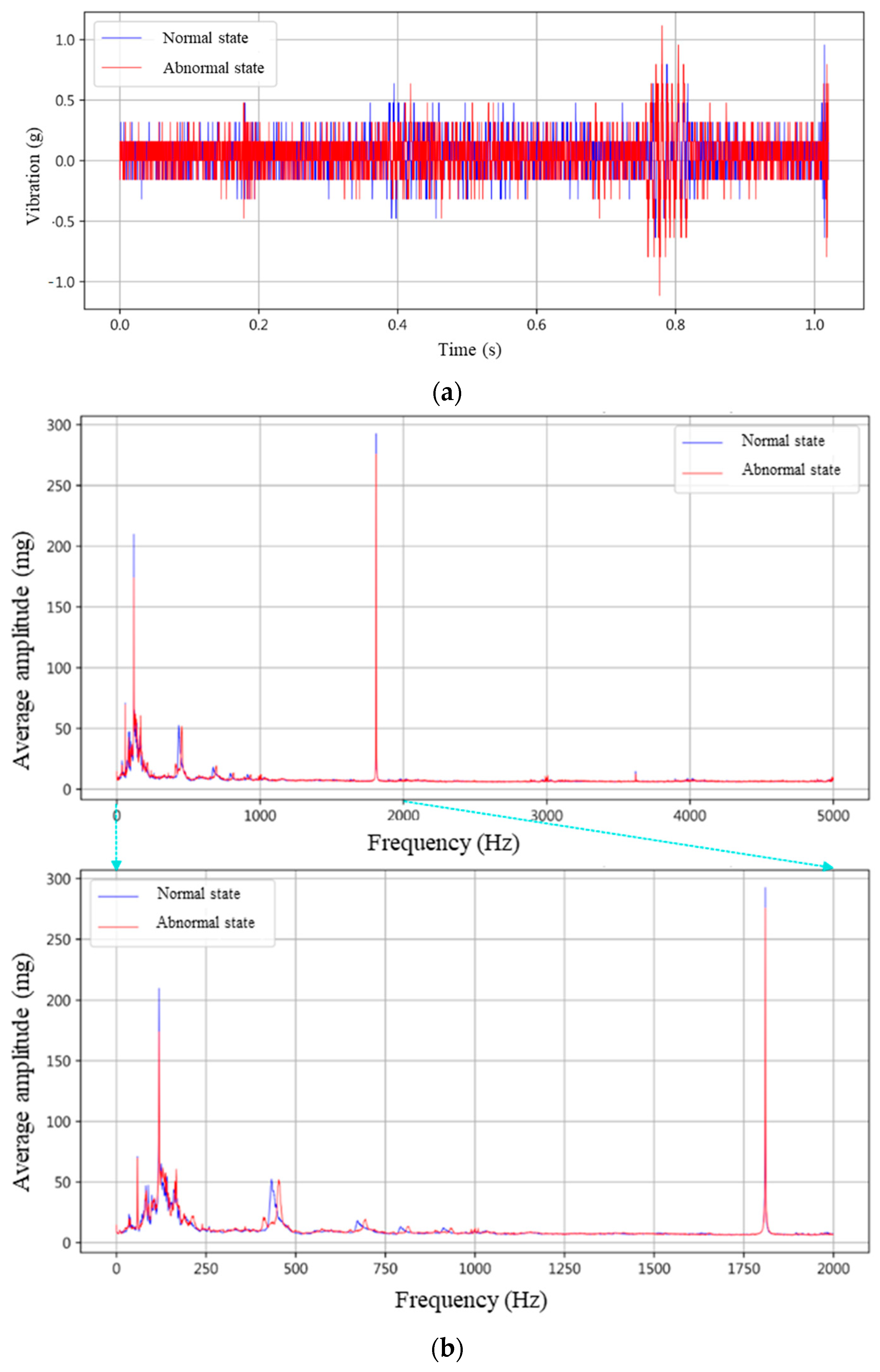
  • Signal type: Various studies have utilized sound, current, and vibration signals for condition monitoring. These signals have been processed and analyzed to distinguish different machine states effectively. Notably, vibration and current signals yield higher classification accuracy compared to sound signals. Vibration signals are also more commonly used in mechanical fault diagnostics. Given these advantages, this study selects voltage singles of vibrations extracted using an accelerometer as the primary signal type.
  • Signal transformation: The raw signals captured by sensors are typically discontinuous time-domain signals. According to the reviewed literature, such signals are challenging to classify directly and require transformation into alternative feature representations for effective model training. Common transformation techniques include converting time-domain signals into frequency-domain features using FFT or employing DWT and STFT for time-frequency analysis. Since the cutting action of the roller laminating machine’s cutter system is completed within approximately one second, frequency-domain analysis provides a more efficient and effective approach for feature extraction.
  • Model type: Machine learning is widely used for classification in PdM. Traditional machine learning models, such as SVM and RF, require manual feature extraction but are effective for smaller datasets. On the other hand, deep learning models, including DNN and CNN, can automatically learn complex patterns from data without extensive feature engineering. These models are particularly useful for capturing nonlinear relationships but require larger datasets and higher computational resources. While deep learning can enhance classification performance, it also introduces challenges such as increased training time and the risk of overfitting when dealing with limited data. Considering the constraints of this study, machine learning methods are chosen as the primary approach for anomaly classification, balancing model complexity with data availability and computational efficiency.
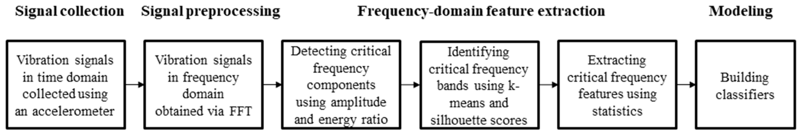
3. Research Methods

This study utilizes an accelerometer to collect data on the cutter system of a roller laminator. As shown in Figure 2, the accelerometer converts vibrations generated during machine operation into voltage signals. Signals were preprocessed and examined in both the time and frequency domains. Feature extraction techniques are applied to identify critical frequency-domain statistics that highlight significant differences between normal and abnormal states. These features serve as the foundation for machine learning models designed to classify cutter conditions.

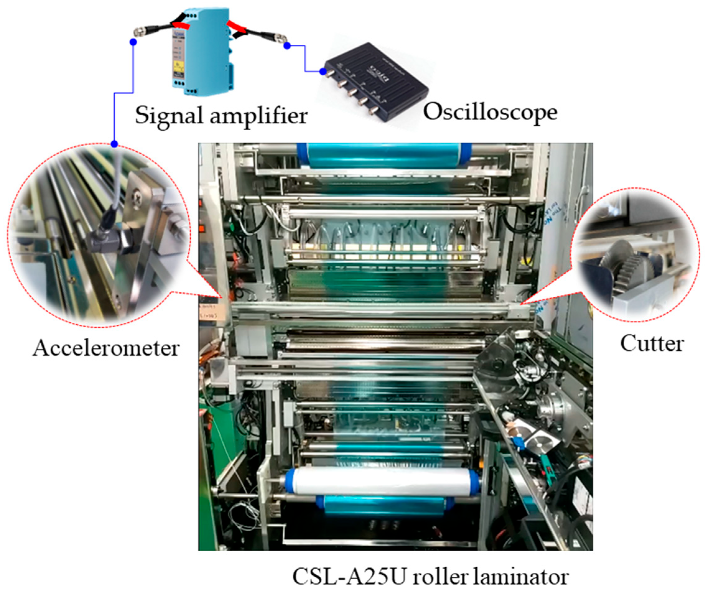
3.1. Hardware Architecture for Singal Collection

This study focuses on extracting vibration singles from the cutter system of the CSL-A25U roller laminator, manufactured by C Sun, Taichung, Taiwan, as shown in Figure 3. A Dytran Instruments 3055D3 accelerometer, manufactured by Dytran Instruments, Inc., Chatsworth, CA, USA, is mounted on the motor drive end of the cutter system using a magnetic base to capture vibration signals in both normal and abnormal conditions. The accelerometer converts mechanical vibrations into voltage signals. It is connected to an ADAM-3017 signal amplifier, manufactured by Advantech Co., Ltd., Taipei, Taiwan, via a sensor connector, which provides power, amplifies the signals, and reduces noise. A high-frequency sampling PicoScope 2406B oscilloscope, from Pico Technology, Cambridgeshire, UK, collects and converts the vibration signals. The processed vibration signals are then stored in an industrial computer running Windows 10 for further analysis.

3.2. Singal Preprocessing

The vibration signals stored by the hardware are in CSV format. Since this study applies supervised learning in machine learning, labeled data are required for model training to enable classification predictions.
In addition, the voltage signals of vibration extracted from the accelerometer belong to the time-domain data. Analyzing vibration signals in the time domain is the most fundamental approach. By examining waveform segments in the time function, various features such as amplitude, waveform shape, periodicity, and trends can be quickly extracted. However, in this study, time-domain analysis alone could not effectively distinguish between normal and abnormal states of the cutter and timing belt tension. Therefore, a signal transformation method was applied to convert the vibration signals of the cutter system into frequency-domain data, from which suitable feature values were extracted.
In signal processing, frequency-domain analysis has become an essential tool. While time-domain analysis provides information on how a signal changes over time, frequency-domain analysis helps identify different frequency components and their amplitudes. The Fourier transform (FT) decomposes any signal into a series of sine and cosine waves, each with a specific frequency and amplitude. This allows complex time-domain signals to be represented as the sum of multiple simple frequency components. With the advancement of digital technology, data captured by sensors undergoes sampling, resulting in discrete time data. The discrete Fourier transform (DFT) converts discrete, non-continuous time-domain signals into the frequency domain, expressed by the following formula:
X k = n = 0 N 1 x n e j 2 π N k n ,
where X [k] represents the k-th frequency component in the frequency domain, x [n] is the n-th discrete sample in the time domain, N is the number of samples (i.e., signal length), and the exponential term serves as the basis function for expanding the time-domain signal into the frequency domain. However, the computational complexity of DFT is O(N2), making it highly expensive as N increases. To address this, the FFT was proposed, which reduces the computational complexity to O(NlogN). The steps for FFT computation are as follows:
  • Step 1: signal decomposition. The time-domain signal of length N is divided into even and odd sequences, as shown in Equations (2) and (3):
x e v e n n = x 2 n
x o d d n = x 2 n + 1
  • Step 2: recursive DFT computation. The even and odd sequences are processed separately using recursive DFT, as expressed in Equations (4) and (5):
X e v e n k = n = 0 N / 2 1 x e v e n n e j 2 π N k n
X o d d k = n = 0 N / 2 1 x o d d n e j 2 π N k n
  • Step 3: sequence combination. As shown in Equation (6), the odd-sequence DFT is rotated using the Twiddle Factor Wk,N = ejk/N and then combined with the even-sequence DFT:
X k = X e v e n k + W k , N X o d d k ,   0 k < N 2 X e v e n k N 2 W k N 2 , N X o d d k N 2 , N 2 k < N

3.3. Frequency-Domain Feature Extraction

Frequency-domain data often exhibits high dimensionality. This makes it challenging to analyze efficiently. Feature extraction in the frequency domain plays a critical role in machine learning applications. It helps eliminate redundant components and noise while preserving essential information. This process enhances model efficiency and accuracy. It does so by reducing computational complexity and improving feature relevance.
  • Step 1: critical frequency component detection. Detecting critical frequency components involves analyzing the frequency domain to extract features that differentiate between normal and abnormal states. The amplitude spectrum is derived using:
A k = R e X k 2 + I m X k 2 ,
where Re (X[k]) and Im (X[k]) represent the real and imaginary components of the complex function, respectively. This transformation helps in understanding the signal’s frequency content. An essential metric for frequency analysis is the energy ratio (ER), which provides insight into the distribution of signal energy across different frequencies. It is computed as
E R k = A k 2 / k A k 2
This study applies mean amplitude difference analysis to distinguish between normal and abnormal states by quantifying spectral variations. The average FFT amplitude is computed for each state, and the amplitude difference is calculated to highlight significant spectral changes. Additionally, mean ER difference analysis is used to evaluate the signal energy distribution. This metric helps assess how energy is distributed across different frequency components and identifies key frequency ranges that contribute to signal characteristics.
  • Step 2: critical frequency band identification. Identifying meaningful frequency bands is essential for effective signal analysis, and clustering techniques play a crucial role in this process. The k-means clustering is employed for its efficiency in partitioning data, with cluster quality evaluated using a widely used metric, silhouette score, which quantifies the cohesion and separation of clusters. The process begins by defining a range of potential cluster numbers, typically from 2 to 10. For each number of clusters, the k-means is applied, and the silhouette score is computed to assess clustering performance. Mathematically, the silhouette score for a clustering result is defined as
S i l h o u e t t e   s c o r e = 1 n i b i a i / m a x a i , b i
where ai is the average distance between the data point i and all other points in the same cluster and bi is the minimum average distance between the data point i and all points in the nearest different cluster. This score measures how well each data point fits within its assigned cluster by comparing the average intra-cluster distance with the nearest-cluster distance. A higher silhouette score, approaching 1, indicates well-separated and compact clusters, while lower values suggest overlapping or poorly defined groupings. By optimizing the number of clusters based on silhouette score, the most meaningful frequency bands can be identified for further analysis.
  • Step 3: critical feature extraction. After frequency-domain analysis identifies critical frequency bands, irrelevant bands are removed to achieve dimensionality reduction. The study further extracts statistical features to extract physically meaningful features for each band, including maximum, mean, standard deviation, skewness, and kurtosis:
m a x i m u m = m a x k X k
μ = k X k / n
σ = k X k μ 2 / n 1
s k e w n e s s = k X k μ 3 / σ 3
k u r t o s i s = k X k μ 4 / σ 4
These extracted features form a structured dataset for subsequent machine learning applications.

3.4. Supervised Machine Learning Algorithms

This study employs three machine learning algorithms: logistic regression (LR), RF, and SVM. The selection of these three models as representatives is based on their ability to cover different types of learning approaches. LR represents a linear model, SVM is a robust boundary-learning model, and RF exemplifies a nonlinear ensemble learning method. These models serve as strong baselines because they are widely used across various domains, including medical diagnosis, fault prediction in manufacturing, and financial risk assessment. Their applicability also varies based on the nature of the data. LR is suitable when the data are linearly separable, SVM is effective when dealing with complex data with a small sample size but high dimensionality, and RF performs well with large datasets that exhibit nonlinear relationships.
The extracted frequency-domain features serve as inputs for these algorithms. Each statistical feature extracted from the critical frequency bands forms a structured feature vector. The machine learning models analyze these feature vectors, learning distinct patterns to accurately differentiate between normal and abnormal states. This structured approach ensures robust and reliable predictive capabilities.

4. Experiment Results

To assess the effectiveness of machine learning models in cutter state prediction, this study conducted experiments under controlled conditions. Since cutter degradation is difficult to detect in the time domain, signal processing techniques were applied to extract distinguishing features. The following sections outline the data collection process, feature extraction methods, and model evaluation results.

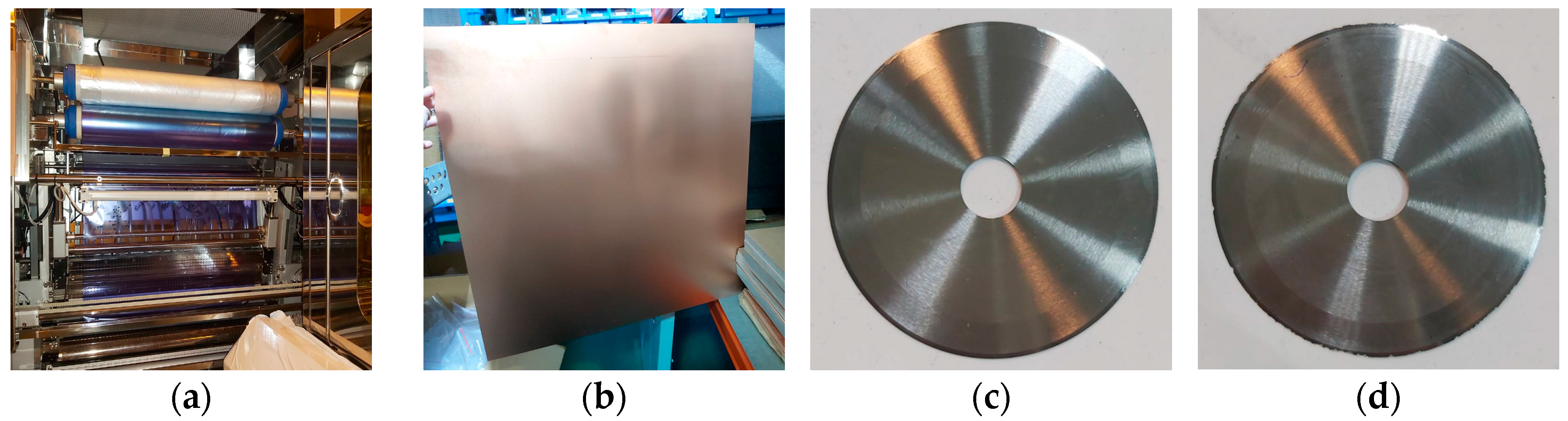
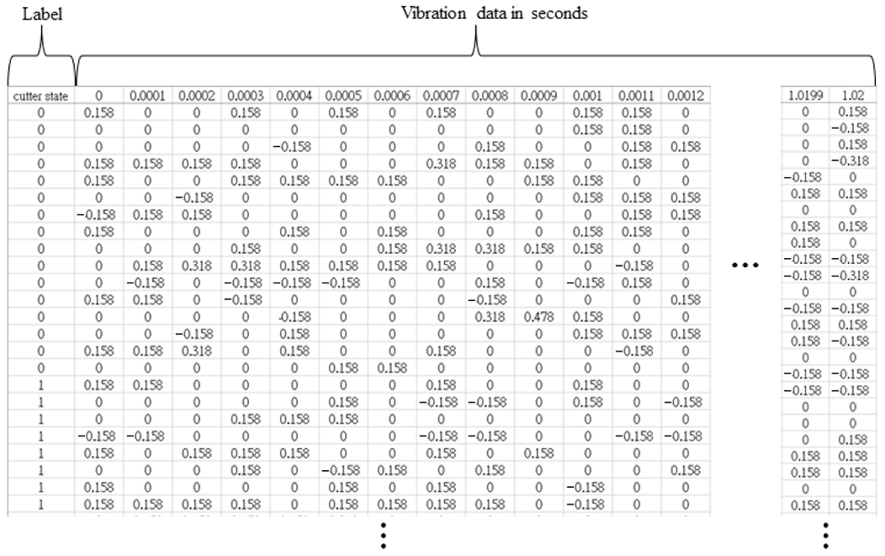
4.1. Data Collection and Labeling

During the production process of the roller laminator, this study used Photec H-7333 dry film and 60 reusable substrates (620 × 620 × 1 mm3) as standard production materials, as shown in Figure 4a,b. Data collection was conducted by manually placing the substrates, allowing them to undergo automatic lamination by the machine. For each laminated substrate, the cutter performs one dry film cutting operation. The PLC inside the equipment controls each cutter action, detecting its start and end points. It then sends signals via a registered jack 45 (RJ45) network cable using the EtherCAT protocol to command the vibration measurement system to begin and stop data acquisition. As a result, each cutter action generates one set of continuous vibration signals, which is stored in the industrial computer.
Since this study aims to predict abnormal cutter conditions, data collection includes both normal and abnormal states, as shown in Figure 4c,d. A normal cutter is defined as a blade that has undergone maintenance and has been used for fewer than 20,000 cycles, maintaining stable cutting performance. An abnormal cutter refers to a blade that has exceeded 100,000 cycles and is near replacement. This condition typically results in poor cutting quality, causing burr formation and incomplete film cutting.
Each cutting operation takes approximately 1.021 s, with a sampling rate of 1/10,000 s per sample. Consequently, each recorded cutter operation contains 10,201 acceleration data points over time. The data presented in the Supplementary Materials were extracted from the industrial computer of the roller laminating machine. It contains a total of 855 records, with 483 labeled as normal and 372 as abnormal. The dataset is split into 70% training data and 30% testing data for model evaluation. Figure 5 shows the structure of the dataset. Rows represent different tools, and columns represent features. The first column states that 0 means normal and 1 means abnormal. Columns 2 to 10,202 represent vibration over time, measured in gravitational acceleration (g).

4.2. Feature Engineering for Vibration Singals

In this study, we randomly selected time-series data within one second for both normal and abnormal cutters in the time domain. We first visualized the data to compare the differences, as shown in Figure 6a. The amplitude and waveform differences between the normal and abnormal states were not significant, making it difficult to clearly distinguish them. Therefore, signal transformation methods were required for further processing.
We then applied the FFT to convert the time-domain signals into frequency-domain signals. As shown in Figure 6b, the total frequency range covered 0 to 5000 Hz, with a vibration energy value recorded every 0.98 Hz. As a result, for each cutting blade action, the FFT-extracted frequency-domain data contained 5101 feature values. The frequency-domain signals were then visualized to analyze the amplitude differences in specific frequency ranges between the normal and abnormal states. As shown in Figure 6b, the amplitude peaks of the frequency-domain signals for the cutters were more prominent between 0 and 2000 Hz.
To further examine this, we focused on the 0–2000 Hz range, as depicted in Figure 6b. Noticeable amplitude differences were observed around 80–160 Hz, 400–500 Hz, and near 1800 Hz.
If the frequency-domain feature data are directly used for machine learning modeling, it would not only increase computational load and processing time but also add complexity to subsequent analysis. To reduce irrelevant frequency-domain feature differences between normal and abnormal states, this section applies two feature extraction methods: state average amplitude difference analysis and energy ratio difference analysis. The top 3% of frequency points with the largest differences from both methods were selected, resulting in 32 key frequencies.
As shown in Figure 7a, the important frequency points with significant differences are marked with red dots using the state average amplitude difference analysis and energy ratio analysis. Next, the 32 key frequencies were fed into k-means clustering to automatically identify critical frequency bands. As depicted in Figure 7b, when the number of clusters was set to three, the silhouette score reached its highest value. These three key frequency bands, highlighted in yellow in Figure 7a, were 89–160 Hz, 410–460 Hz, and 1805–1812 Hz.
Finally, this study extracted 15 statistical features, including maximum value, mean, standard deviation, skewness, and kurtosis, from each key frequency band. These features were used as independent variables for the machine learning model.

4.3. Model Training and Comparison

Since the cutting action of the roller lamination machine’s cutter system is completed within approximately one second, frequency domain analysis allows for a simpler and more efficient signal pattern interpretation. Using FFT, the top 3% of frequency spectrum magnitude differences and spectral energy ratio variations between normal and abnormal cutter states can be extracted as 32 key frequencies for feature selection. Additionally, from these 32 key frequencies, three critical frequency bands can be identified. Statistical features, as defined in Equations (10)–(14), are then extracted from these bands, resulting in a total of 15 features.
However, as discussed in Section 2, the application of wavelet transform (WT) for time-frequency analysis has also gained significant attention. In this study, WT is applied using both DWT and continuous wavelet transform (CWT) to process the signals in the time-frequency domain. In DWT, each sample undergoes wavelet transformation, where the signal is decomposed into approximation coefficients (cA) and detail coefficients (cD). In multi-level wavelet decomposition, cA represents the low-frequency components, capturing the main trend or overall structure of the signal. Meanwhile, cD contains the high-frequency components, which help identify sudden changes, noise, and other variations in the signal. The statistical features extracted from these components include the mean, standard deviation, maximum, minimum, range, and median absolute deviation (MAD), totaling 12 features. In the case of CWT, each sample signal is decomposed across a continuous range of wavelet scales. The scale range extends from 1 to 64, enabling feature extraction from high-frequency to low-frequency signals. For each of these 64 scales, six statistical features are computed, resulting in a total of 384 features. Compared to DWT, CWT provides a finer localization in the time-frequency domain, allowing for a more precise capture of time-varying signals. Consequently, the number of extracted features is significantly higher. FFT primarily emphasizes the concentration of energy in the frequency domain; therefore, maximum, mean, standard deviation, skewness, and kurtosis are selected to describe the shape of the spectral energy distribution. In contrast, DWT and CWT offer multi-scale analysis in both the time and frequency domains, making mean, standard deviation, maximum, minimum, range, and MAD more suitable for capturing vibration variations across different scales.
Based on the aforementioned feature extraction methods, this study incorporates the frequency domain features from FFT, the statistical features from key frequency bands, and the time-frequency features from WT into machine learning models. These extracted features are used to train models, including LR, RF, and SVM.
Table 2 presents a comparative analysis of three different machine learning models applied to four different feature extraction methods: FFT with 32 critical frequencies, FFT with 15 statistical features from 3 critical bands, DWT with 12 statistical features from 2 components, and CWT with 384 statistical features from 64 scales. The models are evaluated based on several classification metrics. Accuracy refers to the overall proportion of correct predictions. Precision indicates how many of the cutters predicted as abnormal are actually abnormal, while recall reflects the model’s ability to correctly identify truly abnormal cases. The F1 score provides a balanced measure of precision and recall. In addition, the results include the number of true positives (TPs), which are cutters with worn blades correctly identified as abnormal. True negatives (TNs) refer to sharp cutters correctly identified as normal. False positives (FPs) are sharp cutters incorrectly classified as worn. False negatives (FNs) are cutters with worn blades that the model failed to detect.
Among the feature extraction methods, FFT-based features, particularly those using statistical features from critical bands, tend to yield the best performance across models. In contrast, DWT-based features generally result in the lowest accuracy and recall, indicating a higher number of false negatives. CWT-based features do not perform as well as FFT-based statistical features. However, they still yield strong results, especially when used with RF and SVM.
When comparing model performance, RF consistently delivers the best overall results across different feature sets. It maintains a good balance between precision and recall. It achieves the best accuracy in most cases, such as 94.16% for FFT with 32 critical frequencies and 93.77% for FFT-based statistical features. SVM, on the other hand, excels in precision, achieving the highest value of 97.73% for FFT with 32 critical frequencies and 95.15% for FFT-based statistical features. However, SVM often sacrifices recall, meaning it is more selective but prone to missing positive cases. In contrast, LR generally exhibits the weakest performance, especially with DWT-based features, though it still provides a reasonable baseline for classification.

5. Conclusions

To address urgent orders, high-quality demands, and labor shortages in the industry, improving equipment utilization, production yield, and lowering the operational skill threshold are key challenges. The PdM and diagnostic functions of process equipment are crucial research topics in the field of AI.
This study focuses on the cutter system of the roller laminating equipment used in the PCB industry. It integrates vibration sensors to extract vibration signals. Using FFT, time-domain signals are converted into frequency-domain signals. Key frequency-domain data are extracted through amplitude variation analysis and energy ratio analysis. Additionally, statistical features of key frequency ranges, DWT-based statistical features, and CWT-based statistical features are obtained. Four different feature extraction methods are applied, combined with three machine learning models, LR, RF, and SVM, for cross-comparison. The goal is to determine the most suitable method for identifying normal and abnormal states of the cutter.
The experimental results for the cutter condition show that, when using 32 key features extracted through amplitude variation and energy ratio analysis, the classification accuracy of LR, RF, and SVM is 88.72%, 94.16%, and 91.44%, respectively. When switching to 15 statistical features of key frequency ranges, the accuracy for RF, LR, and SVM is 87.55%, 93.77%, and 94.94%, respectively. The accuracy of DWT combined with the three machine learning models ranges between 70% and 80%, while CWT achieves 80% to 90%. Based on cross-comparisons, statistical features of key frequency ranges extracted through FFT, combined with SVM, are the most suitable for cutter condition classification.
The cutter system of the roller laminating machine still offers many opportunities for future research on PdM and repair. Areas for further study include the belt, linear bushing, and transmission motor.

Supplementary Materials

The following supporting information can be downloaded at: https://www.mdpi.com/article/10.3390/math13081264/s1.

Author Contributions

Conceptualization, C.-M.J.; methodology, S.-H.C., C.-W.W. and A.P.M.; validation, S.-H.C. and T.-Y.Y.; formal analysis, S.-H.C. and C.-W.W.; data curation, C.-W.W. and C.-M.J.; writing—original draft preparation, S.-H.C., C.-W.W. and T.-Y.Y.; writing—review and editing, A.P.M.; supervision, S.-H.C.; project administration, T.-Y.Y. and S.-H.C.; funding acquisition, S.-H.C. All authors have read and agreed to the published version of the manuscript.

Funding

This research was funded by National Science and Technology Council (NSTC), grant number 113-2221-E-131-031- and The APC was funded by Ming Chi University of Technology.

Data Availability Statement

Data supporting this study are included within the Supplementary Materials.

Conflicts of Interest

The authors declare no conflicts of interest.

References

  1. Achouch, M.; Dimitrova, M.; Ziane, K.; Sattarpanah Karganroudi, S.; Dhouib, R.; Ibrahim, H.; Adda, M. On predictive maintenance in industry 4.0: Overview, models, and challenges. Appl. Sci. 2022, 12, 8081. [Google Scholar] [CrossRef]
  2. Romanssini, M.; de Aguirre, P.C.C.; Compassi-Severo, L.; Girardi, A.G. A review on vibration monitoring techniques for predictive maintenance of rotating machinery. Eng 2023, 4, 1797–1817. [Google Scholar] [CrossRef]
  3. Carvalho, T.P.; Soares, F.A.; Vita, R.; Francisco , P.R.D.; Basto, J.P.; Alcalá, S.G. A systematic literature review of machine learning methods applied to predictive maintenance. Comput. Ind. Eng. 2019, 137, 106024. [Google Scholar] [CrossRef]
  4. Cerrada, M.; Zurita, G.; Cabrera, D.; Sánchez, R.V.; Artés, M.; Li, C. Fault diagnosis in spur gears based on genetic algorithm and random forest. Mech. Syst. Signal Process. 2016, 70, 87–103. [Google Scholar] [CrossRef]
  5. Madhusudana, C.K.; Kumar, H.; Narendranath, S. Face milling tool condition monitoring using sound signal. Int. J. Syst. Assur. Eng. Manag. 2017, 8, 1643–1653. [Google Scholar] [CrossRef]
  6. Kanawaday, A.; Sane, A. Machine learning for predictive maintenance of industrial machines using IoT sensor data. In Proceedings of the 2017 8th IEEE International Conference on Software Engineering and Service Science (ICSESS), Beijing, China, 24–26 November 2017; IEEE: Piscataway, NJ, USA, 2017; pp. 87–90. [Google Scholar]
  7. Madhusudana, C.K.; Gangadhar, N.; Kumar, H.; Narendranath, S. Use of discrete wavelet features and support vector machine for fault diagnosis of face milling tool. Struct. Durab. Health Monit. 2018, 12, 111. [Google Scholar]
  8. Bonci, A.; Longhi, S.; Nabissi, G.; Verdini, F. Predictive maintenance system using motor current signal analysis for industrial robot. In Proceedings of the 2019 24th IEEE International Conference on Emerging Technologies and Factory Automation (ETFA), Zaragoza, Spain, 10–13 September 2019; IEEE: Piscataway, NJ, USA, 2019; pp. 1453–1456. [Google Scholar]
  9. Sikder, N.; Bhakta, K.; Al Nahid, A.; Islam, M.M. Fault diagnosis of motor bearing using ensemble learning algorithm with FFT-based preprocessing. In Proceedings of the 2019 International Conference on Robotics, Electrical and Signal Processing Techniques (ICREST), Dhaka, Bangladesh, 10–12 January 2019; IEEE: Piscataway, NJ, USA, 2019; pp. 564–569. [Google Scholar]
  10. Esakimuthu Pandarakone, S.; Mizuno, Y.; Nakamura, H. A comparative study between machine learning algorithm and artificial intelligence neural network in detecting minor bearing fault of induction motors. Energies 2019, 12, 2105. [Google Scholar] [CrossRef]
  11. Ali, M.Z.; Shabbir, S.K.M.N.; Liang, X.; Zhang, Y.; Hu, T. Machine learning-based fault diagnosis for single-and multi-faults in induction motors using measured stator currents and vibration signals. IEEE Trans. Ind. Appl. 2019, 55, 2378–2391. [Google Scholar] [CrossRef]
  12. Magadán, L.; Suárez, F.J.; Granda, J.C.; García, D.F. Real-time monitoring of electric motors for detection of operating anomalies and predictive maintenance. In Proceedings of the Science and Technologies for Smart Cities: 5th EAI International Summit, SmartCity360, Braga, Portugal, 4–6 December 2019; Springer International Publishing: Cham, Switzerland, 2020; pp. 301–311. [Google Scholar]
  13. Saberi, A.N.; Sandirasegaram, S.; Belahcen, A.; Vaimann, T.; Sobra, J. Multi-sensor fault diagnosis of induction motors using random forests and support vector machine. In Proceedings of the 2020 International Conference on Electrical Machines (ICEM), Gothenburg, Sweden, 23–26 August 2020; IEEE: Piscataway, NJ, USA, 2020; Volume 1, pp. 1404–1410. [Google Scholar]
  14. Pollak, A.; Temich, S.; Ptasiński, W.; Kucharczyk, J.; Gąsiorek, D. Prediction of belt drive faults in case of predictive maintenance in industry 4.0 platform. Appl. Sci. 2021, 11, 10307. [Google Scholar] [CrossRef]
  15. Xiang, C.; Ren, Z.; Shi, P.; Zhao, H. Data-driven fault diagnosis for rolling bearing based on dit-fft and xgboost. Complexity 2021, 2021, 4941966. [Google Scholar] [CrossRef]
  16. Giri, A.; Mehendale, N.; Waghode, N. Optimized fault detection and classification for 3-phase electric drives–an AI/ML approach. In Proceedings of the 2022 International Conference on Innovations in Science and Technology for Sustainable Development (ICISTSD), Kollam, India, 25–26 August 2022; IEEE: Piscataway, NJ, USA, 2022; pp. 80–87. [Google Scholar]
  17. Raouf, I.; Lee, H.; Kim, H.S. Mechanical fault detection based on machine learning for robotic RV reducer using electrical current signature analysis: A data-driven approach. J. Comput. Des. Eng. 2022, 9, 417–433. [Google Scholar] [CrossRef]
  18. Hosseinpour-Zarnaq, M.; Omid, M.; Biabani-Aghdam, E. Fault diagnosis of tractor auxiliary gearbox using vibration analysis and random forest classifier. Inf. Process. Agric. 2022, 9, 60–67. [Google Scholar] [CrossRef]
  19. Aburakhia, S.; Shami, A. SB-PdM: A tool for predictive maintenance of rolling bearings based on limited labeled data. Softw. Impacts 2023, 16, 100503. [Google Scholar] [CrossRef]
  20. Souza, J.C.S.D.; Honorato Júnior, O.; Tiago Filho, G.L.; Carpinteiro, O.A.S.; Biancardine Júnior, H.S.D.; Santos, I.F.S.D. Application of machine learning models in predictive maintenance of Francis hydraulic turbines. Rev. Bras. Recur. Hídricos 2024, 29, e48. [Google Scholar] [CrossRef]
  21. Hakami, A. Strategies for overcoming data scarcity, imbalance, and feature selection challenges in machine learning models for predictive maintenance. Sci. Rep. 2024, 14, 9645. [Google Scholar] [CrossRef] [PubMed]
  22. Khalil, A.F.; Rostam, S. Machine learning-based predictive maintenance for fault detection in rotating machinery: A case study. Eng. Technol. Appl. Sci. Res. 2024, 14, 13181–13189. [Google Scholar] [CrossRef]
Figure 1. Working process of the roller laminating machine.
Mathematics 13 01264 g001
Figure 2. Flowchart of proposed method.
Mathematics 13 01264 g002
Figure 3. Accelerometer installation location.
Mathematics 13 01264 g003
Figure 4. Production materials used in this study. (a) Photec H-7333 dry film; (b) Substrate appearance; (c) Normal cutter; (d) Abnormal cutter with a worn blade.
Mathematics 13 01264 g004
Figure 5. Structure of the dataset.
Mathematics 13 01264 g005
Figure 6. Comparison of signals for different cutter states. (a) In time-domain; (b) In frequency-domain.
Mathematics 13 01264 g006
Figure 7. Detection process of key frequency bands. (a) Average amplitude difference and energy ratio difference analysis of the cutting blade state; (b) Analysis of the optimal number of clusters.
Mathematics 13 01264 g007
Table 1. Overview of feature extraction and methodologies in machine fault diagnosis research.
ReferenceApplication FieldFeature ExtractionMethodology
[4]GearboxTime-domain statistics, FFT, WPTCombined time, frequency, and time-frequency domain features, applied GA for feature reduction, and used RF for classification.
[5]Face milling toolDWT of sound signalCompared multiple classifiers with DT-selected DWT features.
[6]Film-slitting machineDM of time, tension, pressure, width, diameterUsed ARIMA for prediction and four supervised models for classification.
[7]Face milling toolDWT of vibration signalApplied DWT and DT feature selection with SVM for classification.
[8]Belt transmission systemDWT of current signalAnalyzed belt looseness using wavelet energy decomposition.
[9]Motor bearingFFT of vibration signalUsed FFT with normalized features and RF model for fault classification.
[10]BearingFFT of current signalCompared SVM, KNN, and CNN with increasing training data volume.
[11]Induction motorWPT of current and vibration signalsUsed WPT features with SVM and KNN classifiers for fault classification.
[12]PumpFFT of vibration signalCompared FFT-based features of pumps with different maintenance cycles.
[13]Eccentricity faultFFT of current and vibration signalsCombined time- and frequency-domain features, used RF for feature selection, and SVM for classification.
[14]Belt transmission systemFFT of vibration signalUsed autoencoder with FFT features from horizontal and vertical sensors.
[15]BearingFFT of vibration signalUsed FFT features with XGBoost after standardization and parameter tuning.
[16]Stator winding faultsFFT of current and axial flux signalsUsed FFT and PSD features with six classifiers for fault classification.
[17]6-axis robotic armWaveform, statistical, kinetic features of current signalUsed correlation and chi-square tests for feature selection and applied four classifiers.
[18]Tractor gearboxDWT of vibration signalCompared RF and MLP performance with and without CFS feature selection.
[19]BearingFFT, STFT, WPT of vibration signalUsed SB-PdM V1.0 software and similarity metrics for comparison.
[20]Hydraulic turbinesFFT of vibration signalCompared MLP and RBFNN classifiers using FFT features under cavitation and normal states.
[21]Non-woven materials machineryTime-domain raw sensor data of vibration and temperatureGAN-generated data with LSTM features and five classifiers
[22]Rotating machineryFFT of vibration signalFFT-based feature extraction with ensemble classifiers.
Table 2. Performance comparison of pre-classification for cutter states.
FeaturesMetrics
Models
Accuracy (%)Precision (%)Recall (%)F1 Score (%)TPTNFPFN
32 critical frequency from FFTLR88.7285.9886.7986.38921361415
RF94.1693.3392.4592.899814487
SVM91.4497.7381.1388.6686149202
15 statistical features from 3 critical bands of FFTLR87.5584.9184.9184.91901351616
RF93.7792.4592.4592.459814388
SVM94.9495.1592.4593.789814685
12 statistical features from 2 components of DWTLR73.9370.1064.1567.00681193829
RF79.7772.8881.1376.79861222032
SVM78.6071.4380.1975.56851172134
384 statistical features from 64 scales of CWTLR84.0580.3781.1380.75861392021
RF91.4488.8990.5789.72961301012
SVM89.4988.3585.8587.08911391512
Bold text indicates the best-performing model for each performance metric.
Disclaimer/Publisher’s Note: The statements, opinions and data contained in all publications are solely those of the individual author(s) and contributor(s) and not of MDPI and/or the editor(s). MDPI and/or the editor(s) disclaim responsibility for any injury to people or property resulting from any ideas, methods, instructions or products referred to in the content.

