Article

Generalized Grönwall Inequality and Ulam–Hyers Stability in p Space for Fractional Stochastic Delay Integro-Differential Equations

by
Abdelhamid Mohammed Djaouti
1,* and
Muhammad Imran Liaqat
2
1
Department of Mathematics and Statistics, Faculty of Sciences, King Faisal University, Al Hofuf 31982, Saudi Arabia
2
Department of Mathematics, National College of Business Administration & Economics, Lahore 54000, Pakistan
*
Author to whom correspondence should be addressed.
Mathematics 2025, 13(8), 1252; https://doi.org/10.3390/math13081252
Submission received: 2 March 2025 / Revised: 2 April 2025 / Accepted: 9 April 2025 / Published: 10 April 2025

Abstract

:
In this work, we derive novel theoretical results concerning well-posedness and Ulam–Hyers stability. Specifically, we investigate the well-posedness of Caputo–Katugampola fractional stochastic delay integro-differential equations. Additionally, we develop a generalized Grönwall inequality and apply it to prove Ulam–Hyers stability in L p space. Our findings generalize existing results for fractional derivatives and space, as we formulate them in the Caputo–Katugampola fractional derivative and L p space. To support our theoretical results, we present an illustrative example.

1. Introduction

Fractional derivatives extend integer-order derivatives to non-integer orders and describe both the local and global behavior of functions. Unlike ordinary derivatives, which represent instantaneous rates of change and are not aware of past events, fractional derivatives include memory effects and depend on the entire history of a function.
Different types of fractional operators can be found in the literature [1,2,3,4]. Recently, some scholars have incorporated the Caputo–Katugampola fractional derivative (Cap-KFrD) into their research. It interpolates the Caputo fractional derivative (Cap-FrD) and the Caputo–Hadamard fractional derivative (Cap-HFrD). The authors of [5] established an approach to solve for fractional systems using Cap-KFrD. Maa and Chen [6] examined the stability and well-posedness of fractional problems involving Cap-KFrD. Sweilam et al. [7] developed a novel method to solve various problems. Boucenna et al. [8] discussed stability results related to Cap-KFrD. In [9], various inequalities were established using Cap-KFrD. In [10], Hoa et al. explored different concepts regarding the solutions of fuzzy fractional systems with Cap-KFrD. Omaba and Sulaimani [11] presented theoretical results for stochastic problems involving Cap-KFrD. Elbadri [12] found solutions to Burgers’ equation using the Laplace transform in the context of Cap-KFrD. Al-Ghafri et al. [13] conducted a qualitative analysis of integro-differential equations and also obtained solutions using the Adomian approach with Cap-KFrD. For more studies related to Cap-KFrD, see [14,15,16].
Assume that the function is integrable on [ 0 , ϖ ] . The Cap-KFrD of orders 0 < η < 1 and ζ > 0 for the function is given as follows [17]:
D u + η , ζ c l ( c ) = ζ η Γ ( 1 η ) u c l * ( u ) ϝ ( c ) ϝ ( u ) η d u .
The Caputo–Katugampola fractional integral is given as follows [18]:
I u + η , ζ l ( c ) = ζ 1 η Γ ( η ) u c ϝ ( u ) ϝ ( c ) ϝ ( u ) 1 η l ( u ) d u .
The Cap-FrD and Cap-HFrD can be interpolated using the Cap-KFrD: Cap-FrD ( ζ = 1 ) [19] and Cap-HFrD ( ζ 0 + ) [19]. The following graph (Figure 1) illustrates this phenomenon.
Stochastic differential equations are employed to describe systems that are driven by random processes. They are a generalization of classical differential equations with terms describing random noise, usually described by Brownian motion or Wiener processes. These equations have extensive applications in areas such as finance, physics, and biology to model systems that change with time and intrinsic randomness. Fractional differential equations are equations involving derivatives of non-integer order. These equations can be employed to model systems with memory effects or hereditary behavior, where the future state of the system relies on its current and past states. Stochastic fractional differential equations (SFDEs) combine the concept of both stochastic and fractional differential equations to model systems with randomness and memory effects. SFDEs are widely applied in most applications with randomness and memory effects. In biology, SFDEs model anomalous diffusion in cell transport in which molecules exhibit subdiffusive or superdiffusive dynamics due to complex environments. In finance, they model stock price dynamics and interest rate models with long-range dependence in order to enhance the modeling of market memory effects. SFDEs are applied in physics to describe viscoelastic materials in which stress and strain exhibit hereditary characteristics. In hydrology, SFDEs model groundwater flow in porous media with long-term dependence. Additionally, SFDEs are used in engineering for signal processing and control systems. Their ability to account for history-dependent stochasticity makes them effective tools for real-world complex systems.
Fractional stochastic integro-differential equations (FSIDEs) with delay are equations that combine fractional derivatives, stochastic processes, integro-differential terms, and time delays. They are highly suited for modeling intricate systems that display memory dependence, hereditary effects, and randomness. FSIDEs with delay are especially valuable for representing phenomena where retention effects, stochastic dynamics, and inherited characteristics are essential, such as finance, physics, and engineering.
The well-posedness of a fractional-order stochastic system is a fascinating branch of mathematical research. It ensures that such equations have unique solutions that depend continuously on the initial condition. The well-posedness of a fractional-order stochastic system is critical to establishing the equation as a meaningful and reliable mathematical model. Since fractional-order stochastic systems couple both fractional derivatives (which imply memory effects) and stochastic processes (which describe randomness), their solutions must be well defined to remain physically and practically applicable.
Ulam–Hyers stability (UHS) is a crucial principle in the stability analysis of fractional-order stochastic systems, ensuring that small variations in system parameters or initial conditions cause only minimal discrepancies in the solution. This aspect is especially crucial for systems defined by fractional derivatives, which exhibit memory and hereditary properties. Additionally, stochastic effects introducing randomness make stability analysis even more challenging.
In recent years, many scholars have actively worked on various topics related to SFDEs and FSIDEs. In [20], Batiha et al. proposed an innovative approach for solving SFDEs. They formulated a scheme specifically designed to approximate the Riemann–Liouville integral operator, which is subsequently used to obtain approximate solutions for these equations. The authors compared their results with those from the Euler–Maruyama method and the exact solution, highlighting the accuracy and efficiency of their proposed technique. Chen et al. reconstructed a backward equation for SFDEs in [21]. They employed the norm technique to analyze the stability as well as the existence and uniqueness (Ex-Un) of the solution to the backward equation. Moreover, the authors also investigated a simulation case of a European call option using the Euler–Maruyama technique to solve the SFDEs, thus illustrating the applicability of their theoretical results. In [22], Moualkia and Xu conducted a theoretical analysis of variable-order SFDEs. In [23], Ali et al. investigated the coupled system of SFDEs. The article chiefly seeks to find solutions for the coupled system of SFDEs with variable-order derivatives, which will serve as the basis for identifying the necessary conditions for Ex-Un. In this pursuit, the authors utilized the Picard method, which has been shown to work well in this field. The study also serves as the basis for the formulation of Ulam stability conditions for the given model. Li et al. carried out a stability investigation of a system of SFDEs in [24]. The research analyzes the interaction between fractional calculus, stochastic processes, and time delays to provide a better understanding of system stability. It sheds light on the effective solution of these equations via several numerical methods. Moreover, the paper examines both the asymptotic and Lyapunov stability of SFDEs, proposing local stability conditions and examining how delays and fractional orders affect stability characteristics. In [25], Singh et al. investigated the asymptotic stability of SFDEs. The authors of [26] considered a class of SFDEs with variable delay. They employed the Lipschitz condition on the nonlinearity and used the Banach method to obtain their main results. The paper ends with an example showing the theoretical results and exhibiting the applicability of the obtained results in practice. The Euler–Maruyama technique for Caputo SFDEs with coefficients satisfying the linear growth condition and the Lipschitz condition was constructed by Doan et al. in [27]. The authors proved the strong convergence rate of the scheme, especially for time-independent coefficients. Moreover, the article provides findings regarding the convergence and stability of an exponential Euler–Maruyama approach for Caputo SFDEs. Such results further advance the knowledge of numerical solutions for such complicated equations. In [28], the authors conducted an analysis of SFDEs. The Ex-Un of solutions was defined through the Picard scheme. Furthermore, the authors considered the stability of nonlinear SFDEs with Lévy noise, using the Mittag–Leffler function to prove stability. In [29], Li et al. studied Hilfer SFDEs with delay. The Ex-Un of the solutions was then determined by the Picard method and the method of contradiction. Moreover, finite-time stability was investigated using the generalized Grönwall–Bellman inequality. In [30], the authors obtained solutions for FSIDEs using the collocation approach. Cui and Yan [31] discussed the qualitative analysis of FSIDEs. Badr and El-Hoety [32] obtained approximate solutions for FSIDEs using the Galerkin approach. The authors of [33] analyzed the solutions of FSIDEs with the Hilfer fractional operator in L 2 space using the fixed-point approach. For more studies related to SFDEs, see [34,35,36,37,38].
Notable outcomes for FSIDEs with delay concerning Cap-KFrD in L p space are presented in this research work. The Banach fixed-point approach is used to determine the Ex-Un of solutions. By leveraging various inequalities, we derive results concerning the continuous dependence of solutions on initial conditions. In the second part, we formulate a generalized Grönwall inequality for Cap-KFrD and apply it to demonstrate UHS in the L p space. Several fundamental inequalities, including Jensen’s inequality [39], the Burkholder–Davis–Gundy inequality [40], and Hölder’s inequality [41], play a crucial role in substantiating our findings.
Below are some key contributions of our study:
  • As far as we know, this is the first comprehensive analysis of the well-posedness of the solutions of FSIDEs and UHS concerning Cap-KFrD in the L p space.
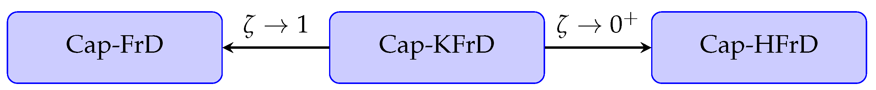
  • We prove all results for the Cap-KFrD, which generalizes Cap-FrD and Cap-HFrD, such that our results are consistent with Cap-FrD when ζ = 1 holds and match with Cap-HFrD when ζ 0 + holds.
  • Most results related to FDSDEs and FSIDEs have been established in the L 2 space; however, we establish these results in the L p space.
  • This research work presents a generalized Grönwall inequality regarding Cap-KFrD.
We examine the following FSIDEs with delay:
{ D 0 + η , ζ c l ( c ) j = 1 e I 0 + U j , ζ Ψ j ( c , l ( c ) ) = J ( c , l ( c ) , l ( c ϱ ) ) + B ( c , l ( c ) , l ( c ϱ ) ) d W ( c ) d c , c [ 0 , ϖ ] , l ( 0 ) = φ ,
where l ( c ) is an R m -valued stochastic process; D 0 + η , ζ c represents the Cap-KFrD with η ( 1 2 , 1 ) , ζ > 0 ; I 0 + U j , ζ is the Caputo–Katugampola fractional integral with 1 2 U j 1 , 1 j e , and ϱ R the delay time; the functions J : [ 0 , ϖ ] × R m × R m R m and B : [ 0 , ϖ ] × R m × R m R m × σ are measurable continuous mappings. The stochastic process ( W c ) c [ 0 , ) follows a standard Brownian trajectory within the σ -dimensional complete filtered probability space ( Ω , F , F = ( F c ) c [ 0 , ) , P ) .
Section 2 defines relevant concepts and presents the fundamental hypothesis that facilitates the basis for the novel results related to well-posedness and UHS of FSIDEs with delay and generalized Grönwall inequality. Section 3 determines the well-posedness of the FSIDEs. Section 4 shows the results of the generalized Grönwall inequality and UHS. Section 5 provides two examples. To conclude, Section 6 outlines our key findings.

2. Preliminaries

This section consists of definition and assumptions that are essentially for establishing important results.
Definition 1. 
Suppose Z c p = L p ( Ω , F c , P ) represents the F c -measurable and p t h integrable functions l = ( l 1 , l 2 , , l m ) T , then Ω R m satisfies
l p = l = 1 m E | l l | p 1 p .
A process conforming to measurability criteria l : [ 0 , ϖ ] L p ( Ω , F c , P ) is referred to as F -adapted subject to l ( c ) Z c p , c 0 . Over each φ Z 0 p , the , which is an F -adapted process, provides the solution of (3) with l ( 0 ) = φ , on the condition that the subsequent (4) is satisfied. This is achieved by applying I 0 + η , ζ on (3).
l ( c ) = φ + j = 1 e 1 Γ ( U j ) 0 c ϝ ( c ) ϝ ( u ) U j 1 ϝ ( u ) Ψ j ( u , l ( u ) ) d u + 1 Γ ( η ) 0 c ( ϝ ( c ) ϝ ( u ) ) η 1 ϝ ( u ) J u , l ( u ) , l ( u γ ) d u + 1 Γ ( η ) 0 c ( ϝ ( c ) ϝ ( u ) ) η 1 ϝ ( u ) B u , l ( u ) , l ( u γ ) d W ( u ) .
For 𝒥 and , assume the following:
  • ( 1 ) δ 1 , δ 2 , V 1 , V 2 R ϰ , there is T such as
    Ψ j ( c , δ 1 ) Ψ j ( c , V 1 ) p +   J ( c , δ 1 , δ 2 ) J ( c , V 1 , V 2 ) p + B ( c , δ 1 , δ 2 ) B ( c , V 1 , V 2 ) p T δ 1 V 1 p +   δ 2 V 2 p , j = 1 , 2 , , e .
  • ( 2 ) The Ψ j ( c , 0 ) , j = 1 , 2 , , e , J ( c , 0 , 0 ) and B ( c , 0 , 0 ) satisfies
    esssu p c [ 0 , ϖ ] Ψ j ( c , 0 ) p < , esssu p c [ 0 , ϖ ] J ( c , 0 , 0 ) p < , esssu p c [ 0 , ϖ ] B ( c , 0 , 0 ) p < .

3. Generalized Results

In the L p space, we establish generalized theorems on Ex-Un and consistent dependence for the solution of delay FSIDEs.
Using the Banach fixed-point technique, we first determine the Ex-Un results for the solutions of delay FSIDEs. For this, we postulate that H p ( [ 0 , ϖ ] ) is the space of all measurable and F ϖ -adapted processes with l H p = esssu p c [ 0 , ϖ ] l ( c ) p < . It is straightforward to prove that H p ( [ 0 , ϖ ] ) , · H p is a complete normed vector space.
Next, describe an operator ψ φ : H p ( [ 0 , ϖ ] ) H p ( [ 0 , ϖ ] ) with ψ φ ( l ( 0 ) ) = φ and
ψ φ ( l ( c ) ) = φ + j = 1 e ζ 1 U j Γ ( U j ) 0 c ϝ ( c ) ϝ ( u ) U j 1 ϝ ( u ) Ψ j ( u , l ( u ) ) d u + ζ 1 η Γ ( η ) 0 c ϝ ( c ) ϝ ( u ) η 1 ϝ ( u ) J u , l ( u ) , l ( u γ ) d u + ζ 1 η Γ ( η ) 0 c ϝ ( c ) ϝ ( u ) η 1 ϝ ( u ) B u , l ( u ) , l ( u γ ) d W ( u ) .
The lemma below plays a crucial role in proving various results.
l 1 + l 2 p p 2 p 1 ( l 1 p p + l 2 p p , l 1 , l 2 R ϰ .
Lemma 1. 
Presume that ( 1 ) and ( 2 ) are valid. Then, ψ φ is well defined.
Proof. 
Suppose l ( c ) H p [ 0 , ϖ ] and c [ 0 , ϖ ] . Based on (7) and (8), we derive
ψ φ ( l ( c ) ) p p 2 2 p 2 φ p p + 2 ( e + 2 ) p ( e + 2 ) j = 1 e ζ 1 U j Γ ( U j ) p 0 c ϝ ( c ) ϝ ( u ) U j 1 ϝ ( u ) Ψ j ( u , l ( u ) ) d u p p + 2 2 p 2 ζ 1 η p ( Γ ( η ) ) p 0 c ϝ ( c ) ϝ ( u ) η 1 J u , l ( u ) , l ( u γ ) ϝ ( u ) d u p p + 2 2 p 2 ζ 1 η p ( Γ ( η ) ) p 0 c ϝ ( c ) ϝ ( u ) η 1 B u , l ( u ) , l ( u γ ) ϝ ( u ) d W ( u ) p p .
By Hölder’s inequality, we have
2 ( e + 2 ) p ( e + 2 ) j = 1 e ζ 1 U j Γ ( U j ) p 0 c ϝ ( c ) ϝ ( u ) U ι 1 ϝ ( u ) Ψ j ( u , l ( u ) ) d u p p 2 ( e + 2 ) p ( e + 2 ) j = 1 e ζ 1 U j Γ ( U j ) p l = 1 m E 0 c ϝ ( c ) ϝ ( u ) U j 1 | Ψ l , j u , l ( u ) | ϝ ( u ) d u p 2 ( e + 2 ) p ( e + 2 ) j = 1 e ζ 1 U j Γ ( U j ) p l = 1 m E ( 0 c ϝ ( c ) ϝ ( u ) ( U j 1 ) p ( p 1 ) ( ϝ ( u ) ) p p 1 d u p 1 0 c | Ψ l , j u , l ( u ) | p d u ) 2 ( e + 2 ) p ( e + 2 ) j = 1 e ζ 1 U j Γ ( U j ) p l = 1 m E ( sup 1 < u c ϝ ( u ) 1 p 1 p 1 0 c ϝ ( c ) ϝ ( u ) ( U j 1 ) p ( p 1 ) ϝ ( u ) d u p 1 0 c | Ψ l , j u , l ( u ) | p d u ) 2 ( e + 2 ) p ( e + 2 ) j = 1 e ζ 1 U j Γ ( U j ) p X p 1 c ζ U j p 1 p 1 p 1 p 1 U j p 1 p 1 0 c Ψ j u , l ( u ) p p d u ,
where X = sup 0 < u c ϝ ( u ) 1 p 1 .
In accordance with ( 1 ) , we have
Ψ j u , l ( u ) p p 2 p 1 Ψ j u , l ( u ) Ψ j ( u , 0 ) p p + Ψ j ( u , 0 ) p p 2 p 1 ( T p l ( u ) p p + Ψ j ( u , 0 ) p p ) .
Hence, we establish
0 c Ψ j u , l ( u ) p p d u 2 p 1 T p esssu p u [ 1 , ϖ ] l ( u ) p p 0 c 1 d u + 2 p 1 0 c Ψ j ( u , 0 ) p p d u 2 p 1 ϖ T p l ( u ) H p p +   2 p 1 0 c Ψ j ( u , 0 ) p p d u .
As a result, we accomplish
2 ( e + 2 ) p ( e + 2 ) j = 1 e ζ 1 U j Γ ( U j ) p 0 c ϝ ( c ) ϝ ( u ) U ι 1 ϝ ( u ) Ψ j ( u , l ( u ) ) d u p p   2 ( e + 2 ) p ( e + 2 ) j = 1 e ζ 1 U j Γ ( U j ) p X p 1 c ζ U j p 1 p 1 p 1 p 1 U j p 1 p 1 2 p 1 ϖ T p l ( u ) H p p + 2 p 1 0 c Ψ j ( u , 0 ) p p d u .
Now, consider the second term of (9). By employing Hölder’s inequality, we obtain the following:
0 c ϝ ( c ) ϝ ( u ) η 1 J u , l ( u ) , l ( u γ ) ϝ ( u ) d u p p   = l = 1 m E | 0 c ϝ ( c ) ϝ ( u ) η 1 | J l u , l ( u ) , l ( u γ ) | ϝ ( u ) d u | p l = 1 m E ( 0 c ϝ ( c ) ϝ ( u ) ( η 1 ) p ( p 1 ) ( ϝ ( u ) ) p p 1 d u p 1 0 c | J l u , l ( u ) , l ( u γ ) | p d u ) l = 1 m E ( sup 0 < u c ϝ ( u ) 1 p 1 p 1 0 c ϝ ( c ) ϝ ( u ) ( η 1 ) p ( p 1 ) ϝ ( u ) d u p 1 0 c | J l u , l ( u ) , l ( u γ ) | p d u ) X p 1 c ζ η p 1 p 1 p 1 p 1 η p 1 p 1 0 c J u , l ( u ) , l ( u γ ) p p d u .
Based on ( 1 ) , we derive
J u , l ( u ) , l ( u γ ) p p 2 p 1 J u , l ( u ) , l ( u γ ) J ( u , 0 , 0 ) p p + J ( u , 0 , 0 ) p p 2 p 1 ( 2 p 1 T p l ( u ) p p + l ( u γ ) p p + J ( u , 0 , 0 ) p p ) .
Consequently, we achieve the following:
0 c J u , l ( u ) , l ( u γ ) p p d u 2 2 p 2 T p ( esssu p u [ 0 , ϖ ] l ( u ) p p + esssu p u [ 0 , ϖ ] l ( u γ ) p p ) 0 c 1 d u + 2 p 1 0 c J ( u , 0 , 0 ) p p d u 2 2 p 2 ϖ T p ( l ( u ) H p p + l ( u γ ) H p p ) + 2 p 1 0 c J ( u , 0 , 0 ) p p d u .
In light of (14) and (16), we determine
0 c ϝ ( c ) ϝ ( u ) η 1 J u , l ( u ) , l ( u γ ) ϝ ( u ) d u p p X p 1 c ζ ( η p 1 ) p 1 p 1 p 1 η p 1 p 1 2 p 1 ( 2 p 1 T p ϖ ( l ( u ) H p p + l ( u γ ) H p p ) + 0 c J ( u , 0 , 0 ) p p d u ) .
Based on ( 2 ) , we derive from (17) that
0 c ϝ ( c ) ϝ ( u ) η 1 J u , l ( u ) , l ( u γ ) ϝ ( u ) d u p p X p 1 c ζ ( η p 1 ) p 1 p 1 p 1 η p 1 p 1 2 p 1 ( 2 p 1 T p ϖ ( l ( u ) H p p + l ( u γ ) H p p ) + ϖ p ) .
Proceeding to the third term of (9), we employ the Burkholder–Davis–Gundy inequality and Hölder’s inequality to obtain the following:
0 c ( c ζ   u ζ ) η 1 B u , l ( u ) , l ( u γ ) ϝ ( u ) d W ( u ) p p = l = 1 m E | 0 c ϝ ( c ) ϝ ( u ) η 1 B l ( u , l ( u ) , l ( u γ ) ϝ ( u ) d W ( u ) | p l = 1 m C p E | 0 c ϝ ( c ) ϝ ( u ) 2 η 2 | B l u , l ( u ) , l ( u γ ) | 2 ϝ ( u ) 2 d u | p 2 l = 1 m C p E 0 c ϝ ( c ) ϝ ( u ) 2 η 2 | B l u , l ( u ) , l ( u γ ) | p ϝ ( u ) 2 d u 0 c ϝ ( c ) ϝ ( u ) 2 η 2 ϝ ( u ) 2 d u p 2 2 l = 1 m C p E 0 c ϝ ( c ) ϝ ( u ) 2 η 2 | B l u , l ( u ) , l ( u γ ) | p ϝ ( u ) 2 d u sup 0 < u c ϝ ( u ) 0 c ϝ ( c ) ϝ ( u ) 2 η 2 ϝ ( u ) d u p 2 2 G p 2 2 C p c ζ 2 η 1 2 η 1 p 2 2 0 c ϝ ( c ) ϝ ( u ) 2 η 2 B u , l ( u , l ( u γ ) p p ϝ ( u ) 2 d u ,
where G = sup 0 < u c ϝ ( u ) and C p = p p + 1 2 ( p 1 ) p 1 p 2 .
Utilizing ( 1 ) and ( 2 ) , we conclude
B u , l ( u ) , l ( u γ ) p p   2 2 p 2 T p l ( u ) p p + l ( u γ ) p p + 2 p 1 B ( u , 0 , 0 ) p p 2 2 p 2 T p l ( u ) p p + l ( u γ ) p p + 2 p 1 p .
Accordingly, we obtain
0 c ϝ ( c ) ϝ ( u ) 2 η 2 B u , l ( u ) , l ( u γ ) p p ϝ ( u ) 2 d u 2 2 p 2 T p 0 c ϝ ( c ) ϝ ( u ) 2 η 2 ( esssu p u [ 0 , ϖ ] l ( u ) p p + esssu p u [ 0 , ϖ ] l ( u γ ) p p ) ϝ ( u ) 2 d u + 2 p 1 p 0 c ϝ ( c ) ϝ ( u ) 2 η 2 ϝ ( u ) 2 d u 2 2 p 2 T p sup 0 < u c ϝ ( u ) 0 c ϝ ( c ) ϝ ( u ) 2 η 2 ( esssu p u [ 0 , ϖ ] l ( u ) p p + esssu p u [ 0 , ϖ ] l ( u γ ) p p ) ϝ ( u ) d u + 2 p 1 p sup 0 < u c ϝ ( u ) 0 c ϝ ( c ) ϝ ( u ) 2 η 2 ϝ ( u ) d u = G 2 p 1 c ζ ( 2 η 1 ) ( 2 η 1 ) ( 2 p 1 T p l ( u ) H p p + l ( u γ ) H p p + p ) .
Hence, the preceding leads to
0 c ϝ ( c ) ϝ ( u ) 2 η 2 B u , l ( u ) , l ( u γ ) p p ϝ ( u ) 2 d u 2 p 1 c ζ ( 2 η 1 ) ( 2 η 1 ) G ( 2 p 1 T p l ( u ) H p p + l ( u γ ) H p p + p ) .
From (19) and (22), we conclude
0 c ϝ ( c ) ϝ ( u ) η 1 B u , l ( u ) , l ( u γ ) ϝ ( u ) d W ( u ) p p G p 2 2 C p c ζ ( 2 η 1 ) ( 2 η 1 ) p 2 2 2 p 1 c ζ ( 2 η 1 ) ( 2 η 1 ) G ( 2 p 1 T p l ( u ) H p p + l ( u γ ) H p p + p ) .
It follows that ψ ( l ( c ) ) H p is finite, thereby fulfilling the needed result. □
The following lemma is important for Ex-Un.
Lemma 2. 
Assume η , λ > 0 , and c [ 0 , ϖ ] , then
I c η , ζ exp λ c ζ exp λ c ζ λ η .
Proof. 
It follows from (2) that
I c η , ζ exp λ c ζ = ζ 1 η Γ ( η ) 0 c ϝ ( c ) ϝ ( u ) η 1 exp λ u ζ ϝ ( u ) d u .
By K = c ζ u ζ ,
I c η , ζ exp λ c ζ = ζ η exp ( λ c ζ ) Γ ( η ) 0 c ζ K η 1 exp ( λ K ) d K .
Apply G = λ K in (24),
I c η , ζ exp λ c ζ = ζ η exp λ c ζ λ η Γ ( η ) 0 λ c ζ G η 1 exp ( G ) d G ζ η exp λ c ζ λ η Γ ( η ) 0 G η 1 exp ( G ) d G = ζ η exp λ c ζ λ η .
This implies that
1 Γ ( η ) 0 c ϝ ( c ) ϝ ( u ) η 1 exp λ u ζ ϝ ( u ) d u exp λ c ζ ζ λ η .
The next lemma deals with the Ex-Un solution of delay FSIDEs.
Theorem 1. 
Let ( 1 ) and ( 2 ) be valid; afterward, delay FSIDEs (3) ensure a unique solution.
Proof. 
Considering · λ , we have
l ( c ) λ = esssu p c [ 0 , ϖ ] l ( c ) p p Λ ( c ) 1 p , λ > 0 ,
where Λ ( c ) = exp ( λ ( c ζ ) ) .
It can be easily demonstrated that · H p and · λ are equivalent. So, H p ( [ 0 , c ] ) , · λ is also complete and normed.
Take the following into account:
κ = ( 2 ( e + 1 ) p ( e + 1 ) j = 1 e ζ 1 U j Γ ( U j ) p G n p 1 T p c ζ ( p U j 2 U j + 1 ) ( p 1 ) p 1 p U j 2 U j + 1 p 1 Γ ( 2 U j 1 ) ζ λ 2 U j 1 + 2 2 p 2 ζ 1 η p ( Γ ( η ) ) p 2 p 1 G n p 1 T p c ζ ( p η 2 η + 1 ) ( p 1 ) p 1 p η 2 η + 1 p 1 + 2 p 1 G p 2 2 c ζ ( 2 η 1 ) ( 2 η 1 ) p 2 2 T p C p G 2 ζ Γ ( 2 η 1 ) λ 2 η 1 ) < 1 .
For l ( c ) , l * ( c ) H p ( [ 0 , ϖ ] ) , we obtain
ψ φ ( l ( c ) ) ψ φ ( l * ( c ) ) p p 2 ( e + 1 ) p ( e + 1 ) j = 1 e ζ 1 U j Γ ( U j ) p 0 c ϝ ( c ) ϝ ( u ) U j 1 Ψ j u , l ( u ) Ψ j u , l * ( u ) ϝ ( u ) d u p p + 2 2 p 2 ζ 1 η p ( Γ ( η ) ) p 0 c ϝ ( c ) ϝ ( u ) η 1 J u , l ( u ) , l ( u γ ) J u , l * ( u ) , l * ( u γ ) ϝ ( u ) d u p p + + 2 2 p 2 ζ 1 η p ( Γ ( η ) ) p 0 c ϝ ( c ) ϝ ( u ) η 1 B u , l ( u ) , l ( u γ ) B u , l * ( u ) , l * ( u γ ) ϝ ( u ) d W ( u ) p p .
Through the use of Hölder’s inequality and ( 1 ) , we achieve
2 ( e + 1 ) p ( e + 1 ) j = 1 e ζ 1 U j Γ ( U j ) p 0 c ϝ ( c ) ϝ ( u ) U j 1 Ψ j u , l ( u ) Ψ j u , l * ( u ) ϝ ( u ) d u p p = 2 ( e + 1 ) p ( e + 1 ) j = 1 e ζ 1 U j Γ ( U j ) p l = 1 m E | 0 c ϝ ( c ) ϝ ( u ) U j 1 Ψ l , j u , l ( u ) Ψ l , j u , l * ( u ) ϝ ( u ) d u | p 2 ( e + 1 ) p ( e + 1 ) j = 1 e ζ 1 U j Γ ( U j ) p l = 1 m E ( ( 0 c ϝ ( c ) ϝ ( u ) ( U j 1 ) ( p 2 ) p 1 ϝ ( u ) p 2 p 1 d u ) p 1 ( 0 c ϝ ( c ) ϝ ( u ) 2 U j 2 | Ψ l , j u , l ( u ) Ψ l , j u , l * ( u ) ) | ϝ ( u ) d u ) 2 ( e + 1 ) p ( e + 1 ) j = 1 e ζ 1 U j Γ ( U j ) p l = 1 m E ( ( sup 1 < u c ϝ ( u ) 1 1 p 0 c ϝ ( c ) ϝ ( u ) ( U j 1 ) ( p 2 ) p 1 ϝ ( u ) d u ) p 1 ( 0 c ϝ ( c ) ϝ ( u ) 2 U j 2 | Ψ l , j u , l ( u ) Ψ l , j ( u , l * ( u ) ) | ϝ ( u ) 2 d u ) ) 2 ( e + 1 ) p ( e + 1 ) j = 1 e ζ 1 U j Γ ( U j ) p n p 1 T p c ζ ( p U j 2 U j + 1 ) ( p 1 ) p 1 p U j 2 U j + 1 p 1 sup 1 < u c ϝ ( u ) 0 c ϝ ( c ) ϝ ( u ) 2 U j 2 l ( u ) l * ( u ) p p ϝ ( u ) d u ,
where n = sup 0 < u c ϝ ( u ) 1 1 p .
Accordingly, we find
2 ( e + 1 ) p ( e + 1 ) j = 1 e ζ 1 U j Γ ( U j ) p 0 c ϝ ( c ) ϝ ( u ) U j 1 Ψ j u , l ( u ) Ψ j u , l * ( u ) ϝ ( u ) d u p p 2 ( e + 1 ) p ( e + 1 ) j = 1 e ζ 1 U j Γ ( U j ) p G n p 1 T p c ζ ( p U j 2 U j + 1 ) ( p 1 ) p 1 p U j 2 U j + 1 p 1 0 c ϝ ( c ) ϝ ( u ) 2 U j 2 esssu p c [ 0 , ϖ ] l ( u ) l * ( u ) p p exp ( λ ( u ζ ) ) exp ( λ ( u ζ ) ) ϝ ( u ) d u .
Following (30), we deduce:
2 ( e + 1 ) p ( e + 1 ) j = 1 e ζ 1 U j Γ ( U j ) p 0 c ϝ ( c ) ϝ ( u ) U j 1 Ψ j u , l ( u ) Ψ j u , l * ( u ) 1 u d u p p 2 ( e + 1 ) p ( e + 1 ) j = 1 e ζ 1 U j Γ ( U j ) p G n p 1 T p c ζ ( p U j 2 U j + 1 ) ( p 1 ) p 1 p U j 2 U j + 1 p 1 0 c ϝ ( c ) ϝ ( u ) 2 U j 2 l ( u ) l * ( u ) λ p exp ( λ ( u ζ ) ) ϝ ( u ) d u 2 ( e + 1 ) p ( e + 1 ) j = 1 e ζ 1 U j Γ ( U j ) p G n p 1 T p c ζ ( p U j 2 U j + 1 ) ( p 1 ) p 1 p U j 2 U j + 1 p 1 l ( u ) l * ( u ) λ p Γ ( 2 U j 1 ) ζ exp ( λ c ζ ) λ 2 U j 1 .
Proceeding with the second term of (28) and employing Hölder’s inequality and ( 1 ) , we obtain:
0 c ϝ ( c ) ϝ ( u ) η 1 J u , l ( u ) , l ( u γ ) J u , l * ( u ) , l * ( u γ ) ϝ ( u ) d u p p = l = 1 m E | 0 c ϝ ( c ) ϝ ( u ) η 1 J l u , l ( u ) , l ( u γ ) J l u , l * ( u ) , l * ( u γ ) ϝ ( u ) d u | p l = 1 m E ( ( 0 c ϝ ( c ) ϝ ( u ) ( η 1 ) ( p 2 ) p 1 ϝ ( u ) p 2 p 1 d u ) p 1 ( 0 c ϝ ( c ) ϝ ( u ) 2 η 2 | J l u , l ( u ) , l ( u γ ) J l ( u , l * ( u ) , l * ( u γ ) ) | p ϝ ( u ) 2 d u ) ) l = 1 m E ( ( sup 0 < u c ϝ ( u ) 1 1 p 0 c ϝ ( c ) ϝ ( u ) ( η 1 ) ( p 2 ) p 1 ϝ ( u ) d u ) p 1 ( 0 c ϝ ( c ) ϝ ( u ) 2 η 2 | J l u , l ( u ) , l ( u γ ) J l ( u , l * ( u ) , l * ( u γ ) ) | p ϝ ( u ) 2 d u ) ) 2 p 1 n p 1 T p c ζ ( p η 2 η + 1 ) ( p 1 ) p 1 p η 2 η + 1 p 1 sup 0 < u c ϝ ( u ) 0 c ϝ ( c ) ϝ ( u ) 2 η 2 l ( u ) l * ( u ) p p + l ( u γ ) l * ( u γ ) p p ϝ ( u ) d u .
It follows that
0 c ϝ ( c ) ϝ ( u ) η 1 J u , l ( u ) , l ( u γ ) J u , l * ( u ) , l * ( u γ ) ϝ ( u ) d u p p 2 p 1 G n p 1 T p c ζ ( p η 2 η + 1 ) ( p 1 ) p 1 p η 2 η + 1 p 1 0 c ϝ ( c ) ϝ ( u ) 2 η 2 l ( u ) l * ( u ) p p + l ( u γ ) l * ( u γ ) p p ϝ ( u ) d u .
Continuing with the third term of (28) and applying the Burkholder–Davis–Gundy inequality and ( 1 ) , we derive
0 c ϝ ( c ) ϝ ( u ) η 1 B u , l ( u ) , l ( u γ ) B u , l * ( u ) , l * ( u γ ) ϝ ( u ) d W ( u ) p p = l = 1 m E | 0 c ϝ ( c ) ϝ ( u ) η 1 B l u , l ( u ) , l ( u γ ) B l u , l * ( u ) , l * ( u γ ) ϝ ( u ) d W ( u ) | p l = 1 m C p E | 0 c ϝ ( c ) ϝ ( u ) 2 η 2 | B l u , l ( u ) , l ( u γ ) B l u , l * ( u ) , l * ( u γ ) | 2 ϝ ( u ) 2 d u | p 2 l = 1 m C p E 0 c ϝ ( c ) ϝ ( u ) 2 η 2 | B l u , l ( u ) , l ( u γ ) B l u , l * ( u ) , l * ( u γ ) | p ϝ ( u ) 2 d u 0 c ϝ ( c ) ϝ ( u ) 2 η 2 ϝ ( u ) 2 d u p 2 2 l = 1 m C p E 0 c ϝ ( c ) ϝ ( u ) 2 η 2 | B l u , l ( u ) , l ( u γ ) B l u , l * ( u ) , l * ( u γ ) | p ϝ ( u ) 2 d u sup 0 < u c ϝ ( u ) 0 c ϝ ( c ) ϝ ( u ) 2 η 2 ϝ ( u ) d u p 2 2 2 p 1 G p 2 2 c ζ ( 2 η 1 ) ( 2 η 1 ) p 2 2 T p C p 0 c ϝ ( c ) ϝ ( u ) 2 η 2 l ( u ) l * ( u ) p p + l ( u γ ) l * ( u γ ) p p ϝ ( u ) 2 d u 2 p 1 G p 2 2 ( c ζ ) ( 2 η 1 ) ( 2 η 1 ) p 2 2 T p C p sup 0 < u c ϝ ( u ) 0 c ϝ ( c ) ϝ ( u ) 2 η 2 l ( u ) l * ( u ) p p + l ( u γ ) l * ( u γ ) p p ϝ ( u ) d u .
Accordingly, we derive
0 c ϝ ( c ) ϝ ( u ) η 1 B u , l ( u ) , l ( u γ ) B u , l * ( u ) , l * ( u γ ) ϝ ( u ) d W ( u ) p p 2 p 1 G p 2 2 c ζ ( 2 η 1 ) ( 2 η 1 ) p 2 2 T p C p G 0 c ϝ ( c ) ϝ ( u ) 2 η 2 l ( u ) l * ( u ) p p + l ( u γ ) l * ( u γ ) p p ϝ ( u ) d u .
From (28), we arrive at
ψ φ l ( c ) ψ φ l * ( c ) p p 2 ( e + 1 ) p ( e + 1 ) j = 1 e ζ 1 U j Γ ( U j ) p G n p 1 T p c ζ ( p U j 2 U j + 1 ) ( p 1 ) p 1 p U j 2 U j + 1 p 1 l ( u ) l * ( u ) λ p Γ ( 2 U j 1 ) ζ exp ( λ c ζ ) λ 2 U j 1 + 2 2 p 2 ζ 1 η p ( Γ ( η ) ) p 2 p 1 G n p 1 T p c ζ ( p η 2 η + 1 ) ( p 1 ) p 1 p η 2 η + 1 p 1 + 2 p 1 G p 2 2 c ζ ( 2 η 1 ) ( 2 η 1 ) p 2 2 T p C p G 0 c l ( u ) l * ( u ) p p + l ( u γ ) l * ( u γ ) p p ϝ ( c ) ϝ ( u ) 2 η 2 ϝ ( u ) d u .
Following (35), we establish
ψ φ l ( c ) ψ φ l * ( c ) p p exp ( λ ( c ζ ) ) 1 exp ( λ ( c ζ ) ) 2 ( e + 1 ) p ( e + 1 ) j = 1 e ζ 1 U j Γ ( U j ) p G n p 1 T p c ζ ( p U j 2 U j + 1 ) ( p 1 ) p 1 p U j 2 U j + 1 p 1 l ( u ) l * ( u ) λ p Γ ( 2 U j 1 ) ζ exp ( λ c ζ ) λ 2 U j 1 + 1 exp ( λ ( c ζ ) ) 2 2 p 2 ζ 1 η p ( Γ ( η ) ) p 2 p 1 G n p 1 T p c ζ ( p η 2 η + 1 ) ( p 1 ) p 1 p η 2 η + 1 p 1 + 2 p 1 G p 2 2 c ζ ( 2 η 1 ) ( 2 η 1 ) p 2 2 T p C p G 0 c l ( u ) l * ( u ) p p exp ( λ ( u ζ ) ) exp ( λ ( u ζ ) ) + l ( u γ ) l * ( u γ ) p p exp ( λ ( u γ ) ζ ) exp ( λ ( u γ ) ζ ) ϝ ( c ) ϝ ( u ) 2 η 2 ϝ ( u ) d u 2 ( e + 1 ) p ( e + 1 ) j = 1 e ζ 1 U j Γ ( U j ) p G n p 1 T p c ζ ( p U j 2 U j + 1 ) ( p 1 ) p 1 p U j 2 U j + 1 p 1 l ( u ) l * ( u ) λ p Γ ( 2 U j 1 ) ζ λ 2 U j 1 + 1 exp ( λ ( c ζ ) ) 2 2 p 2 ζ 1 η p ( Γ ( η ) ) p 2 p 1 G n p 1 T p c ζ ( p η 2 η + 1 ) ( p 1 ) p 1 p η 2 η + 1 p 1 + 2 p 1 G p 2 2 c ζ ( 2 η 1 ) ( 2 η 1 ) p 2 2 T p C p G 0 c exp ( λ ( c ζ ) ) esssu p u [ 0 , ϖ ] l ( u ) l * ( u ) p p exp ( λ ( c ζ ) ) + exp ( λ ( u γ ) ζ ) esssu p u [ 0 , ϖ ] l ( u γ ) l * ( u γ ) p p exp ( λ ( u γ ) ζ ) ϝ ( c ) ϝ ( u ) 2 η 2 ϝ ( u ) d u 2 ( e + 1 ) p ( e + 1 ) j = 1 e ζ 1 U j Γ ( U j ) p G n p 1 T p c ζ ( p U j 2 U j + 1 ) ( p 1 ) p 1 p U j 2 U j + 1 p 1 l ( u ) l * ( u ) λ p Γ ( 2 U j 1 ) ζ exp ( λ c ζ ) λ 2 U j 1 + 1 exp ( λ ( c ζ ) ) 2 2 p 2 ζ 1 η p ( Γ ( η ) ) p 2 p 1 G n p 1 T p c ζ ( p η 2 η + 1 ) ( p 1 ) p 1 p η 2 η + 1 p 1 + 2 p 1 G p 2 2 c ζ ( 2 η 1 ) ( 2 η 1 ) p 2 2 T p C p G l ( c ) l * ( c ) λ p 0 c ϝ ( c ) ϝ ( u ) 2 η 2 exp ( λ ( u ζ ) ) + exp ( λ ( u γ ) ζ ) ϝ ( u ) d u 2 ( e + 1 ) p ( e + 1 ) j = 1 e ζ 1 U j Γ ( U j ) p G n p 1 T p c ζ ( p U j 2 U j + 1 ) ( p 1 ) p 1 p U j 2 U j + 1 p 1 l ( u ) l * ( u ) λ p Γ ( 2 U j 1 ) ζ λ 2 U j 1 + 1 exp ( λ ( c ζ ) ) 2 2 p 2 ζ 1 η p ( Γ ( η ) ) p 2 p 1 G n p 1 T p c ζ ( p η 2 η + 1 ) ( p 1 ) p 1 p η 2 η + 1 p 1 + 2 p 1 G p 2 2 c ζ ( 2 η 1 ) ( 2 η 1 ) p 2 2 T p C p G 2 l ( c ) l * ( c ) λ p 0 c ϝ ( c ) ϝ ( u ) 2 η 2 ϝ ( u ) exp ( λ ( u ζ ) ) d u 2 ( e + 1 ) p ( e + 1 ) j = 1 e ζ 1 U j Γ ( U j ) p G n p 1 T p c ζ ( p U j 2 U j + 1 ) ( p 1 ) p 1 p U j 2 U j + 1 p 1 l ( u ) l * ( u ) λ p Γ ( 2 U j 1 ) ζ λ 2 U j 1 + 2 2 p 2 ζ 1 η p ( Γ ( η ) ) p 2 p 1 G n p 1 T p c ζ ( p η 2 η + 1 ) ( p 1 ) p 1 p η 2 η + 1 p 1 + 2 p 1 G p 2 2 c ζ ( 2 η 1 ) ( 2 η 1 ) p 2 2 T p C p G 2 l ( c ) l * ( c ) λ p Γ ( 2 η 1 ) ζ λ 2 η 1 .
Accordingly, from (36), we get
ψ φ l ( c ) ψ φ l * ( c ) λ p ( 2 ( e + 1 ) p ( e + 1 ) j = 1 e ζ 1 U j Γ ( U j ) p G n p 1 T p c ζ ( p U j 2 U j + 1 ) ( p 1 ) p 1 p U j 2 U j + 1 p 1 Γ ( 2 U j 1 ) ζ λ 2 U j 1 + 2 2 p 2 ζ 1 η p ( Γ ( η ) ) p ( 2 p 1 G n p 1 T p c ζ ( p η 2 η + 1 ) ( p 1 ) p 1 p η 2 η + 1 p 1 + 2 p 1 G p 2 2 c ζ ( 2 η 1 ) ( 2 η 1 ) p 2 2 T p C p G ) 2 ζ Γ ( 2 η 1 ) λ 2 η 1 ) l ( c ) l * ( c ) λ p .
Consequently, we acquire
ψ φ l ( c ) ψ φ l * ( c ) λ κ 1 p l ( c ) l * ( c ) λ .
From (27), we have κ < 1 . Therefore, we have demonstrated the required result. □
Theorem 2. 
Given any φ , φ , the following statement holds:
B η ( c , φ ) B η ( c , φ ) | p T φ φ p , c [ 0 , ϖ ] ;
here, B η ( c , φ ) is the solution.
Proof. 
It follows that
B η ( c , φ ) B η ( c , φ ) = φ φ + j = 1 e ζ 1 U j Γ ( U j ) 0 c ϝ ( c ) ϝ ( u ) U j 1 Ψ j ( u , B η ( u , φ ) ) Ψ j ( u , B η ( u , φ ) ) ϝ ( u ) d u + 1 Γ ( η ) 0 c ϝ ( c ) ϝ ( u ) η 1 J ( u , B η ( u , φ ) , B η ( u γ , φ ) ) J ( u , B η ( u , φ ) , B η ( u γ , φ ) ) ϝ ( u ) d u + 1 Γ ( η ) 0 c ϝ ( c ) ϝ ( u ) η 1 B ( u , B η ( u , φ ) , B η ( u γ , φ ) ) B ( u , B η ( u , φ ) , B η ( u γ , φ ) ) ϝ ( u ) d W ( u ) .
By applying (8) to (40), we arrive at
B η ( c , φ ) B η ( c , φ ) p p 2 p 1 φ φ p p + 2 ( e + 2 ) p ( e + 2 ) j = 1 e ζ 1 U j Γ ( U j ) p 0 c ϝ ( c ) ϝ ( u ) U j 1 Ψ j u , B ( u , φ ) Ψ j ( u , B ( u , φ ) ) ϝ ( u ) d u p p + 2 3 p 3 ( Γ ( η ) ) p 0 c ϝ ( c ) ϝ ( u ) η 1 ( J ( u , B η ( u , φ ) , B η ( u γ , φ ) ) J u , B η ( u , φ ) , B η ( u γ , φ ) ) ϝ ( u ) d u p p + 2 3 p 3 ( Γ ( η ) ) p 0 c ϝ ( c ) ϝ ( u ) η 1 ( B u , B η ( u , φ ) , B η ( u γ , φ ) ) B u , B η ( u , φ ) , B η ( u γ , φ ) ) ϝ ( u ) d W ( u ) p p .
From the Hölder’s inequality and ( 1 ) , it follows that
2 ( e + 2 ) p ( e + 2 ) j = 1 e ζ 1 U j Γ ( U j ) p 0 c ϝ ( c ) ϝ ( u ) U j 1 Ψ j ( u , B ( u , φ ) ) Ψ j ( u , B ( u , φ ) ) ϝ ( u ) d u p p = 2 ( e + 2 ) p ( e + 2 ) j = 1 e ζ 1 U j Γ ( U j ) p l = 1 m E | 0 c ϝ ( c ) ϝ ( u ) U j 1 Ψ l , j u , B ( u , φ ) Ψ l , j u , B ( u , φ ) ϝ ( u ) d u | p 2 ( e + 2 ) p ( e + 2 ) j = 1 e ζ 1 U j Γ ( U j ) p l = 1 m E ( ( 0 c ϝ ( c ) ϝ ( u ) ( U j 1 ) ( p 2 ) p 1 ϝ ( u ) p 2 p 1 d u ) p 1 ( 0 c ϝ ( c ) ϝ ( u ) 2 U j 2 | Ψ l , j u , B ( u , φ ) Ψ l , j ( u , B ( u , φ ) ) | ϝ ( u ) d u ) ) 2 ( e + 2 ) p ( e + 2 ) j = 1 e ζ 1 U j Γ ( U j ) p l = 1 m E ( ( sup 1 < u c ϝ ( u ) 1 1 p 0 c ϝ ( c ) ϝ ( u ) ( U j 1 ) ( p 2 ) p 1 ϝ ( u ) d u ) p 1 ( 0 c ϝ ( c ) ϝ ( u ) 2 U j 2 | Ψ l , j ( u , B ( u , φ ) ) Ψ l , j ( u , B ( u , φ ) ) | ϝ ( u ) 2 d u ) ) 2 ( e + 2 ) p ( e + 2 ) j = 1 e ζ 1 U j Γ ( U j ) p n p 1 T p c ζ ( p U j 2 U j + 1 ) ( p 1 ) p 1 p U j 2 U j + 1 p 1 sup 1 < u c ϝ ( u ) 0 c ϝ ( c ) ϝ ( u ) 2 U j 2 B ( u , φ ) B ( u , φ ) p p ϝ ( u ) d u .
Consequently, we derive
2 ( e + 2 ) p ( e + 2 ) j = 1 e ζ 1 U j Γ ( U j ) p 0 c ϝ ( c ) ϝ ( u ) U j 1 Ψ j ( u , B η ( u , φ ) ) Ψ j u , B ( u , φ ) ϝ ( u ) d u p p 2 ( e + 2 ) p ( e + 2 ) j = 1 e ζ 1 U j Γ ( U j ) p G n p 1 T p c ζ ( p U j 2 U j + 1 ) ( p 1 ) p 1 p U j 2 U j + 1 p 1 0 c ϝ ( c ) ϝ ( u ) 2 U j 2 B ( u , φ ) B ( u , φ ) p p ϝ ( u ) d u .
By applying Hölder’s inequality and ( 1 ) to the second term of (41), it follows that
0 c ϝ ( c ) ϝ ( u ) η 1 ( J ( u , B η ( u , φ ) , B η ( u γ , φ ) ) J u , B η ( u , φ ) , B η ( u γ , φ ) ) ϝ ( u ) d u p p = l = 1 m E | 0 c ϝ ( c ) ϝ ( u ) η 1 ( J l ( u , B η ( u , φ ) , B η ( u γ , φ ) ) J l u , B η ( u , φ ) , B η ( u γ , φ ) ) ϝ ( u ) d u | p l = 1 m E ( ( 0 c ϝ ( c ) ϝ ( u ) ( η 1 ) ( p 2 ) p 1 ϝ ( u ) p 2 p 1 d u ) p 1 ( 0 c ϝ ( c ) ϝ ( u ) 2 η 2 | J l ( u , B η ( u , φ ) , B η ( u γ , φ ) ) J l ( u , B η ( u , φ ) , B η ( u γ , φ ) ) | ϝ ( u ) 2 d u ) ) l = 1 m E ( ( sup 0 < u c ϝ ( u ) 1 1 p 0 c ϝ ( c ) ϝ ( u ) ( η 1 ) ( p 2 ) p 1 ϝ ( u ) d u ) p 1 ( 0 c ϝ ( c ) ϝ ( u ) 2 η 2 | J l ( u , B η ( u , φ ) , B η ( u γ , φ ) ) J l ( u , B η ( u , φ ) , B η ( u γ , φ ) ) | ϝ ( u ) 2 d u ) ) 2 p 1 n p 1 T p c ζ ( p η 2 η + 1 ) ( p 1 ) p 1 p η 2 η + 1 p 1 0 c ϝ ( c ) ϝ ( u ) 2 η 2 B η ( u , φ ) B η ( u , φ ) p p + B η ( u γ , φ ) B η ( u γ , φ ) p p ϝ ( u ) 2 d u . 2 p 1 n p 1 T p c ζ ( p η 2 η + 1 ) ( p 1 ) p 1 p η 2 η + 1 p 1 sup 0 < u c ϝ ( u ) 0 c ϝ ( c ) ϝ ( u ) 2 η 2 B η ( u , φ ) B η ( u , φ ) p p + B η ( u γ , φ ) B η ( u γ , φ ) p p ϝ ( u ) d u = 2 p 1 n p 1 T p c ζ ( p η 2 η + 1 ) ( p 1 ) p 1 p η 2 η + 1 p 1 G 0 c ϝ ( c ) ϝ ( u ) 2 η 2 B η ( u , φ ) B η ( u , φ ) p p + B η ( u γ , φ ) B η ( u γ , φ ) p p ϝ ( u ) d u .
Using the Burkholder–Davis–Gundy inequality and ( 1 ) for the third term of (41), we conclude that
0 c ϝ ( c ) ϝ ( u ) η 1 ( B ( u , B η ( u , φ ) , B η ( u γ , φ ) ) B u , B η ( u , φ ) , B η ( u γ , φ ) ) ϝ ( u ) d W ( u ) p p = l = 1 m E | 0 c ϝ ( c ) ϝ ( u ) η 1 ( B l ( u , B η ( u , φ ) , B η ( u γ , φ ) ) B l u , B η ( u , φ ) , B η ( u γ , φ ) ) ϝ ( u ) d W ( u ) | p l = 1 m C p E | 0 c ϝ ( c ) ϝ ( u ) 2 η 2 | B l ( u , B η ( u , φ ) , B η ( u γ , φ ) ) B l ( u , B η ( u , φ ) , B η ( u γ , φ ) ) | 2 ϝ ( u ) 2 d u | p 2 l = 1 m C p E 0 c ϝ ( c ) ϝ ( u ) 2 η 2 | B l ( u , B η ( u , φ ) , B η ( u γ , φ ) ) B l ( u , B η ( u , φ ) , B η ( u γ , φ ) ) | p ϝ ( u ) 2 d u 0 c ϝ ( c ) ϝ ( u ) 2 η 2 ϝ ( u ) 2 d u p 2 2 l = 1 m C p E 0 c ϝ ( c ) ϝ ( u ) 2 η 2 | B l ( u , B η ( u , φ ) , B η ( u γ , φ ) ) B l ( u , B η ( u , φ ) , B η ( u γ , φ ) ) | p ϝ ( u ) 2 d u sup 0 < u c ϝ ( u ) 0 c ϝ ( c ) ϝ ( u ) 2 η 2 ϝ ( u ) d u p 2 2 2 p 1 G p 2 2 T p C p ( c ζ ) ( 2 η 1 ) ( 2 η 1 ) p 2 2 0 c ϝ ( c ) ϝ ( u ) 2 η 2 B η ( u , φ ) B η ( u , φ ) p p + B η ( u γ , φ ) B η ( u γ , φ ) p p ϝ ( u ) 2 d u . 2 p 1 G p 2 2 T p C p ( c ζ ) ( 2 η 1 ) ( 2 η 1 ) p 2 2 sup 0 < u c ϝ ( u ) 0 c ϝ ( c ) ϝ ( u ) 2 η 2 B η ( u , φ ) B η ( u , φ ) p p + B η ( u γ , φ ) B η ( u γ , φ ) p p ϝ ( u ) d u . = 2 p 1 G p 2 2 T p C p ( c ζ ) ( 2 η 1 ) ( 2 η 1 ) p 2 2 G 0 c ϝ ( c ) ϝ ( u ) 2 η 2 B η ( u , φ ) B η ( u , φ ) p p + B η ( u γ , φ ) B η ( u γ , φ ) p p ϝ ( u ) d u .
By considering (41), (43), (44), and (45), we establish
B η ( c , φ )   B η ( c , φ ) λ p 2 p 1 exp ( λ ( c ζ ) ) φ φ p p + 2 p 1 κ B η ( u , φ ) B η ( u , φ ) λ p
Accordingly, we conclude
B η ( c , φ ) B η ( c , φ ) λ p ( 1 2 p 1 κ ) 2 p 1 exp ( λ ( c ζ ) ) φ φ p p
Thus, we acquire the following required result:
lim φ φ B η ( c , φ ) B η ( c , φ ) λ p = 0 .

4. Stability Results

In this section, we first establish a generalized Grönwall inequality concerning Cap-KFrD and then demonstrate the UHS of the FSIDEs in L p space.
Lemma 3. 
Assume the functions M ( c ) > 0 and L ( c ) > 0 are locally integrable on c [ m , ϖ )   ( m 0 , ϖ + ) , and further, consider the continuous and nondecreasing mapping of Z : [ m , ϖ ) [ 0 , θ ] , θ R + .
If the following holds,
L ( c ) M ( c ) + ζ 1 η Z ( c ) Γ ( η ) m c ϝ ( c ) ϝ ( u ) η 1 ϝ ( u ) L ( u ) d u , c [ m , ϖ ) ,
then
L ( c ) M ( c ) + m c r = 0 ( ζ 1 η Z ( c ) ) r Γ ( r η ) ϝ ( c ) ϝ ( u ) r η 1 M ( u ) ϝ ( u ) d u , c [ m , ϖ ) .
Proof. 
For locally integrable function ϱ , assume
ρ ϱ ( c ) = ζ 1 η Z ( c ) Γ ( η ) m c ϝ ( c ) ϝ ( u ) η 1 ϝ ( u ) ϱ ( u ) d u .
So, we obtain
L ( c ) M ( c ) + ρ L ( c ) ;
therefore,
L ( c ) ι = 0 r 1 ρ ι M ( c ) + ρ L r ( c ) .
We need to prove that
ρ r L ( c ) 0 c ( ζ 1 η Z ( c ) ) η Γ ( r η ) ϝ ( c ) ϝ ( u ) r η 1 ϝ ( u ) L ( u ) d u
and ρ r L ( c ) 0 when r c [ m , ϖ ) .
Inequality (47) holds when r = 1 . Suppose it is also for r = ι . Now, we will prove that it is true for r = ι + 1
ρ ι + 1 L ( c ) = ρ ( ρ ι L ( c ) ) ζ 1 η Z ( c ) Γ ( η ) 0 c ϝ ( c ) ϝ ( u ) η 1 ϝ ( u ) 0 u ( ζ 1 η Z ( c ) ) ι Γ ( ι η ) ( u ζ c ζ ) ι η 1 c ζ 1 L ( c ) d c d u ( Z ( c ) ) ι + 1 Γ ( η ) 0 c ϝ ( c ) ϝ ( u ) η 1 ϝ ( u ) 0 u ( ζ 1 η ) ι Γ ( ι η ) ( u ζ c ζ ) ι η 1 c ζ 1 L ( c ) d c d u .
It follows that we have the following:
ρ ι + 1 L ( c ) 0 c ( Z ( c ) ζ 1 η ) ι + 1 Γ ( ( ι + 1 ) η ) ϝ ( c ) ϝ ( u ) ( ι + 1 ) η 1 ϝ ( u ) L ( u ) d u .
Accordingly, inequality (47) is verified. Proceeding further, from inequality (47), we arrive at the following:
ρ r L ( c ) 0 c ( ζ 1 η ϖ ) r Γ ( r η ) ϝ ( c ) ϝ ( u ) r η 1 ϝ ( u ) L ( u ) d u 0
when r + for c [ m , ϖ ) ; this finalizes the proof. □
In the case of Z ( c ) = b in Lemma 3, we deduce the following inequality.
Corollary 1. 
Assume that b 0 , η > 0 , and M ( c ) is a locally integrable non-negative mapping with 0 c < ϖ , ( ϖ + ) . Further, let L ( c ) be a locally integrable and non-negative mapping for 0 c < ϖ . Then, we have
L ( c ) M ( c ) + b 0 c ϝ ( c ) ϝ ( u ) η 1 ϝ ( u ) L ( u ) d u ,
and then,
L ( c ) M ( c ) + 0 c r = 0 ( b Γ ( η ) ) r Γ ( r η ) ϝ ( c ) ϝ ( u ) r η 1 M ( u ) ϝ ( u ) d u , 0 c < ϖ .
Corollary 2. 
Under the same conditions of Lemma 3, assume M ( c ) is a nondecreasing mapping with [ 0 , ϖ ) . Then, we get the following:
L ( c ) M ( c ) E η Z ( c ) Γ ( η ) ( c ζ ) η ;
where E η is the Mittag-Leffler function defined by E η ( c ) = ι = 0 c ι Γ ( ι η + 1 ) .
Proof. 
By the hypotheses
L ( c ) M ( c ) 1 + 0 c r = 1 Z ( c ) Γ ( η ) r Γ ( r η ) ϝ ( c ) ϝ ( u ) r η 1 ϝ ( u ) d u = M ( c ) r = 0 Z ( c ) Γ ( η ) ( c ζ ) η r Γ ( r η + 1 ) = M ( c ) E η Z ( c ) Γ ( η ) ( c ζ ) η .
This concludes the proof. □
Definition 2. 
(3) is UHS with respect to ε if there exists V > 0 so that for all ε > 0 and for all G H p ( 0 , ϖ ) , with G ( 0 ) = G 0 , of
E ( G ( c ) G ( 0 ) ( j = 1 e ζ 1 U j Γ ( U j ) 0 c ϝ ( c ) ϝ ( u ) U j 1 ϝ ( u ) Ψ j ( u , G ( u ) ) d u + ζ 1 η Γ ( η ) 0 c ϝ ( c ) ϝ ( u ) η 1 ϝ ( u ) J u , G ( u ) , G ( u γ ) d u + ζ 1 η Γ ( η ) 0 c ϝ ( c ) ϝ ( u ) η 1 ϝ ( u ) B u , G ( u ) , G ( u γ ) d W ( u ) ) p p ) < ε , c [ 0 , ϖ ] ,
there exists a solution U H p ( 0 , ϖ ) of (3), with U ( c ) = G 0 when c [ 0 , ϖ ] , and satisfies the following:
E G ( c ) U ( c ) p p V ε , c [ 0 , ϖ ] .
In the following theorem, we establish UHS for the FSIDEs with delay.
Theorem 3. 
Suppose ( 1 ) and ( 2 ) hold, then system (3) is UHS on [ 0 , ϖ ] .
Proof. 
Assume ε > 0 and G H p ( 0 , ϖ ) is the solution of (49), and assume U H p ( 0 , ϖ ) is the solution of (3) with initial condition U ( 0 ) = G 0 ; then, we have
U ( c ) = G ( 0 ) + j = 1 e ζ 1 U j Γ ( U j ) 0 c ϝ ( c ) ϝ ( u ) U j 1 ϝ ( u ) Ψ j ( u , U ( u ) ) d u + ζ 1 η Γ ( η ) 0 c ϝ ( c ) ϝ ( u ) η 1 ϝ ( u ) J u , U ( u ) , U ( u γ ) d u + ζ 1 η Γ ( η ) 0 c ϝ ( c ) ϝ ( u ) η 1 ϝ ( u ) B u , U ( u ) , U ( u γ ) d W ( u ) .
So, we obtain
G ( c ) U ( c ) = G ( c ) G ( 0 ) ( j = 1 e ζ 1 U j Γ ( U j ) 0 c ϝ ( c ) ϝ ( u ) U j 1 ϝ ( u ) Ψ j ( u , G ( u ) ) d u + ζ 1 η Γ ( η ) 0 c ϝ ( c ) ϝ ( u ) η 1 ϝ ( u ) J u , G ( u ) , G ( u γ ) d u + ζ 1 η Γ ( η ) 0 c ϝ ( c ) ϝ ( u ) η 1 ϝ ( u ) B u , G ( u ) , G ( u γ ) d W ( u ) ) + j = 1 e ζ 1 U j Γ ( U j ) 0 c ϝ ( c ) ϝ ( u ) U j 1 ϝ ( u ) Ψ j ( u , G ( u ) ) Ψ j ( u , U ( u ) ) d u ζ 1 η Γ ( η ) 0 c ϝ ( c ) ϝ ( u ) η 1 ϝ ( u ) J u , G ( u ) , G ( u γ ) J u , U ( u ) , U ( u γ ) d u ζ 1 η Γ ( η ) 0 c ϝ ( c ) ϝ ( u ) η 1 ϝ ( u ) B u , G ( u ) , G ( u γ ) B u , U ( u ) , U ( u γ ) d W ( u ) .
Making use of Jensen’s inequality, Hölder’s inequality, and the Burkholder–Davis–Gundy inequality, we deduce the following:
E G ( c ) U ( c ) p p 2 p 1 E ( G ( c ) G ( 0 ) ( j = 1 e ζ 1 U j Γ ( U j ) 0 c ϝ ( c ) ϝ ( u ) U j 1 ϝ ( u ) Ψ j ( u , G ( u ) ) d u + ζ 1 η Γ ( η ) 0 c ϝ ( c ) ϝ ( u ) η 1 ϝ ( u ) J u , G ( u ) , G ( u γ ) d u + ζ 1 η Γ ( η ) 0 c ϝ ( c ) ϝ ( u ) η 1 ϝ ( u ) B u , G ( u ) , G ( u γ ) d W ( u ) ) p p ) + 2 p 1 E ( j = 1 e ζ 1 U j Γ ( U j ) 0 c ϝ ( c ) ϝ ( u ) U j 1 ϝ ( u ) Ψ j ( u , G ( u ) ) Ψ j ( u , U ( u ) ) d u ζ 1 η Γ ( η ) 0 c ϝ ( c ) ϝ ( u ) η 1 ϝ ( u ) J u , G ( u ) , G ( u γ ) J u , U ( u ) , U ( u γ ) d u ζ 1 η Γ ( η ) 0 c ϝ ( c ) ϝ ( u ) η 1 ϝ ( u ) B u , G ( u ) , G ( u γ ) B u , U ( u ) , U ( u γ ) d W ( u ) ) p p 2 p 1 ε + 2 ( e + 2 ) p ( e + 2 ) E j = 1 e ζ 1 U j Γ ( U j ) 0 c ϝ ( c ) ϝ ( u ) U j 1 ϝ ( u ) Ψ j ( u , G ( u ) ) Ψ j ( u , U ( u ) ) d u p p + 6 p 1 E ζ 1 η Γ ( η ) 0 c ϝ ( c ) ϝ ( u ) η 1 ϝ ( u ) J u , G ( u ) , G ( u γ ) J u , U ( u ) , U ( u γ ) d u p p + 6 p 1 E ζ 1 η Γ ( η ) 0 c ϝ ( c ) ϝ ( u ) η 1 ϝ ( u ) B u , G ( u ) , G ( u γ ) B u , U ( u ) , U ( u γ ) d W ( u ) p p 2 p 1 ε + 2 ( e + 2 ) p ( e + 2 ) j = 1 e ζ 1 U j Γ ( U j ) p X p 1 c ζ U j p 1 p 1 p 1 p 1 U j p 1 p 1 0 c Ψ j ( u , G ( u ) Ψ j u , U ( u ) p p d u + 6 p 1 p 1 c ζ η p 1 p 1 p 1 p 1 η p 1 p 1 0 c J u , G ( u ) , G ( u γ ) J u , U ( u ) , U ( u γ ) p p d u + 6 p 1 G p 2 2 C p c ζ 2 η 1 2 η 1 p 2 2 0 c ϝ ( c ) ϝ ( u ) 2 η 2 B u , G ( u , G ( u γ ) B u , U ( u , U ( u γ ) p p ϝ ( u ) 2 d u 2 p 1 ε + 2 ( e + 2 ) p ( e + 2 ) T p j = 1 e ζ 1 U j Γ ( U j ) p X p 1 c ζ U j p 1 p 1 p 1 p 1 U j p 1 p 1 0 c G ( u ) U ( u ) p p d u + 12 p 1 T p p 1 c ζ η p 1 p 1 p 1 p 1 η p 1 p 1 0 c G ( u ) U ( u ) p p + U ( u γ ) U ( u γ ) p p d u + 12 p 1 T p G p 2 2 C p c ζ 2 η 1 2 η 1 p 2 2 sup 1 < u c ϝ ( u ) 0 c ϝ ( c ) ϝ ( u ) 2 η 2 G ( u ) U ( u ) p p + U ( u γ ) U ( u γ ) p p ϝ ( u ) d u .
Assume that
Θ ( c ) = esssu p c [ 0 , ϖ ] E G ( c ) U ( c ) p p , c [ 0 , ϖ ] ,
we get E G ( c ) U ( c ) p p Θ ( c ) and E G ( c γ ) U ( c γ ) p p Θ ( c ) when c [ 0 , ϖ ] . Accordingly, we derive the following:
E G ( c ) U ( c ) p p 2 p 1 ε + 2 ( e + 2 ) p ( e + 2 ) T p j = 1 e ζ 1 U j Γ ( U j ) p X p 1 c ζ U j p 1 p 1 p 1 p 1 U j p 1 p 1 0 c Θ ( u ) d u + 12 p 1 T p p 1 c ζ η p 1 p 1 p 1 p 1 η p 1 p 1 2 0 c Θ ( u ) d u + 12 p 1 T p G p 2 2 C p c ζ 2 η 1 2 η 1 p 2 2 2 G 0 c ϝ ( c ) ϝ ( u ) 2 η 2 Θ ( u ) ϝ ( u ) d u .
From (53), we derive the following:
Θ ( c ) ( 2 p 1 ε + 2 ( e + 2 ) p ( e + 2 ) T p j = 1 e ζ 1 U j Γ ( U j ) p X p 1 c ζ U j p 1 p 1 p 1 p 1 U j p 1 p 1 + 12 p 1 T p p 1 c ζ η p 1 p 1 p 1 p 1 η p 1 p 1 2 ) 0 c Θ ( u ) d u + 12 p 1 T p G p 2 2 C p c ζ 2 η 1 2 η 1 p 2 2 2 G 0 c ϝ ( c ) ϝ ( u ) 2 η 2 Θ ( u ) ϝ ( u ) d u .
With the help of the generalized Grönwall inequality, we deduce from (54)
Θ ( c ) { 2 p 1 ε + ( 2 ( e + 2 ) p ( e + 2 ) T p j = 1 e ζ 1 U j Γ ( U j ) p X p 1 c ζ U j p 1 p 1 p 1 p 1 U j p 1 p 1 + 12 p 1 T p p 1 c ζ η p 1 p 1 p 1 p 1 η p 1 p 1 2 ) 0 c Θ ( u ) d u } × E 2 η 1 , 1 12 p 1 T p G p 2 2 C p c ζ 2 η 1 2 η 1 p 2 2 2 G Γ ( 2 η 1 ) c ζ ( 2 η 1 ) = Υ 1 ε + Υ 2 0 c Θ ( u ) d u , c [ 0 , ϖ ] ,
where
Υ 1 = 2 p 1 E 2 η 1 , 1 12 p 1 T p G p 2 2 C p c ζ 2 η 1 2 η 1 p 2 2 2 G Γ ( 2 η 1 ) c ζ ( 2 η 1 ) ,
and
Υ 2 = 12 p 1 T p p 1 c ζ η p 1 p 1 p 1 p 1 η p 1 p 1 2 ) × E 2 η 1 , 1 12 p 1 T p G p 2 2 C p c ζ 2 η 1 2 η 1 p 2 2 2 G Γ ( 2 η 1 ) c ζ ( 2 η 1 ) .
By utilizing Grönwall inequality, we arrive at
Θ ( c ) Υ 1 ε exp ( Υ 2 c ) Υ 1 ε exp ( Υ 2 ϖ ) = V ε .
Consequently, the final expression is
E G ( c ) U ( c ) p p V ε , c [ 0 , ϖ ] .
This implies that (3) is UHS with ε . □
Remark 1. 
The convergence order for UHS is linear, as the power of ε in the stability bound is one.
Remark 2. 
When the model contains small delays, UHS becomes more likely to hold. However, the stability properties fundamentally depend on the magnitude of the delay and the specific characteristics of the problem. For a comprehensive analysis of how delays affect UHS, see [42,43].

5. Example

In this section, we provide an example to demonstrate our theoretical results.
Example 1. 
Examine the following:
D 0 + η , ζ c l ( c ) I 0 + U 1 , ζ 5 c sin ( l ( c ) ) I 0 + U 2 , ζ 4 cos ( l ( c ) ) = 3 cos ( l ( c ) ) sin ( l ( c 1 5 ) ) + 4 sin ( l ( c ) ) cos ( l ( c 1 5 ) ) d W ( c ) d c , c [ 0 , 6 ] , l ( 0 ) = φ ,
where e = 2 , ϖ = 6 , Ψ 1 ( c , l ( c ) ) = 5 c sin ( l ( c ) ) , Ψ 2 ( c , l ( c ) ) = 4 cos ( l ( c ) ) ,
J ( c , l ( c ) , l ( c ϱ ) ) = 3 cos ( l ( c ) ) sin ( l ( c 1 5 ) ) , B ( c , l ( c ) , l ( c ϱ ) ) = 4 sin ( l ( c ) ) cos ( l ( c 1 5 ) ) .
We compute the following:
Ψ 1 ( c , Φ 1 ( c ) ) Ψ 1 ( c , Φ 2 ( c ) )     5 Φ 1 ( c ) ) Φ 2 ( c ) ) ,
Ψ 2 ( c , Φ 1 ( c ) ) Ψ 2 ( c , Φ 2 ( c ) )     4 Φ 1 ( c ) ) Φ 2 ( c ) ) ,
J ( c , Φ 1 ( c ) , Φ 1 ( c ϱ ) ) J ( c , Φ 2 ( c ) , Φ 2 ( c ϱ ) )     3 Φ 1 ( c ) ) Φ 2 ( c ) ) + Φ 1 ( c ϱ ) Φ 2 ( c ϱ ) ,
B ( c , Φ 1 ( c ) , Φ 1 ( c ϱ ) ) B ( c , Φ 2 ( c ) , Φ 2 ( c ϱ ) )     4 Φ 1 ( c ) ) Φ 2 ( c ) ) + Φ 1 ( c ϱ ) Φ 2 ( c ϱ ) .
Accordingly, condition ( 1 ) is achieved with T = 5 . Likewise, for j = 1 , 2 , we achieve esssu p c [ 0 , 6 ] Ψ j ( c , 0 ) p < 5 , esssu p c [ 0 , 6 ] J ( c , 0 , 0 ) p < 5 , and esssu p c [ 0 , 6 ] B ( c , 0 , 0 ) p < 5 . Consequently, Theorem 1 guarantees the Ex-Un of the solution for System (55). Furthermore, by Theorem 3, System (55) is UHS, as we have demonstrated that conditions ( 1 ) and ( 2 ) are satisfied.

6. Conclusions

This study introduces new findings on the solution’s Ex-Un and its persistent dependence on the initial value for FSIDEs with delay. Additionally, we derive a generalized Grönwall inequality and prove UHS. All these results are presented in the L p space and the context of Cap-KFrD. In this way, we make significant contributions to the literature. Applying several important inequalities, such as Jensen’s inequality, the Burkholder–Davis–Gundy inequality, and Hölder’s inequality, is a key tool used to prove the theorems and lemmas. In the future, we will develop a financial model using SFDEs that incorporate both fractional Brownian motion and standard Brownian motion.

Author Contributions

Conceptualization, A.M.D. and M.I.L.; methodology, A.M.D. and M.I.L.; software, A.M.D. and M.I.L.; validation, A.M.D. and M.I.L.; formal analysis, A.M.D. and M.I.L.; investigation, A.M.D. and M.I.L.; resources, A.M.D.; writing—original draft preparation, A.M.D. and M.I.L.; writing—review and editing, A.M.D. and M.I.L.; visualization, A.M.D. and M.I.L.; funding acquisition, A.M.D. All authors have read and agreed to the published version of the manuscript.

Funding

This work was supported by the Deanship of Scientific Research, Vice Presidency for Graduate Studies and Scientific Research, King Faisal University, Saudi Arabia (Project No. KFU251299).

Data Availability Statement

No data were generated or analyzed during the current study.

Conflicts of Interest

The authors declare no conflicts of interest.

Abbreviations

The following abbreviations are used in this manuscript:
Cap-KFrDCaputo–Katugampola fractional derivative
Cap-FrDCaputo fractional derivative
Cap-HFrDCaputo–Hadamard fractional derivative
Ex-UnExistence and uniqueness
SFDEsStochastic fractional differential equations
FSIDEsFractional stochastic integro-differential equations
UHSUlam–Hyers stability

References

  1. Subramanian, M.; Manigandan, M.; Zada, A.; Gopal, T.N. Existence and Hyers-Ulam stability of solutions for nonlinear three fractional sequential differential equations with nonlocal boundary conditions. Int. J. Nonlinear Sci. Numer. Simul. 2024, 24, 3071–3099. [Google Scholar] [CrossRef]
  2. Mohammed Djaouti, A.; Khan, Z.A.; Imran Liaqat, M.; Al-Quran, A. A novel technique for solving the nonlinear fractional-order smoking model. Fractal Fract. 2024, 8, 286. [Google Scholar] [CrossRef]
  3. Gunasekar, T.; Raghavendran, P.; Santra, S.S.; Majumder, D.; Baleanu, D.; Balasundaram, H. Application of Laplace transform to solve fractional integro-differential equations. J. Math. Comput. Sci. 2024, 33, 225–237. [Google Scholar] [CrossRef]
  4. Din, A.; Li, Y.; Khan, F.M.; Khan, Z.U.; Liu, P. On Analysis of fractional order mathematical model of Hepatitis B using Atangana–Baleanu Caputo (ABC) derivative. Fractals 2022, 30, 2240017. [Google Scholar] [CrossRef]
  5. Zeng, S.; Baleanu, D.; Bai, Y.; Wu, G. Fractional differential equations of Caputo-Katugampola type and numerical solutions. Appl. Math. Comput. 2017, 315, 549–554. [Google Scholar] [CrossRef]
  6. Ma, L.; Chen, Y. Analysis of Caputo–Katugampola fractional differential system. Eur. Phys. J. Plus 2024, 139, 171. [Google Scholar] [CrossRef]
  7. Sweilam, N.H.; Nagy, A.M.; Al-Ajami, T.M. Numerical solutions of fractional optimal control with Caputo–Katugampola derivative. Adv. Differ. Equ. 2021, 2021, 425. [Google Scholar] [CrossRef]
  8. Boucenna, D.; Ben Makhlouf, A.; Naifar, O.; Guezane-Lakoud, A.; Hammami, M.A. Linearized stability analysis of Caputo-Katugampola fractional-order nonlinear systems. J. Nonlinear Funct. Anal. 2018, 2018, 27. [Google Scholar]
  9. Nazeer, N.; Asjad, M.I.; Azam, M.K.; Akgül, A. Study of results of katugampola fractional derivative and chebyshev inequailities. Int. J. Appl. Comput. Math. 2022, 8, 225. [Google Scholar] [CrossRef]
  10. Van Hoa, N.; Vu, H.; Duc, T.M. Fuzzy fractional differential equations under Caputo–Katugampola fractional derivative approach. Fuzzy Sets Syst. 2019, 375, 70–99. [Google Scholar]
  11. Omaba, M.E.; Sulaimani, H.A. On Caputo–Katugampola fractional stochastic differential equation. Mathematics 2022, 10, 2086. [Google Scholar] [CrossRef]
  12. Elbadri, M. An approximate solution of a time fractional Burgers’ equation involving the Caputo-Katugampola fractional derivative. Partial. Differ. Equations Appl. Math. 2023, 8, 100560. [Google Scholar] [CrossRef]
  13. Al-Ghafri, K.S.; Alabdala, A.T.; Redhwan, S.S.; Bazighifan, O.; Ali, A.H.; Iambor, L.F. Symmetrical solutions for non-local fractional integro-differential equations via caputo–katugampola derivatives. Symmetry 2023, 15, 662. [Google Scholar] [CrossRef]
  14. Sadek, L.; Jarad, F. The general Caputo–Katugampola fractional derivative and numerical approach for solving the fractional differential equations. Alex. Eng. J. 2025, 121, 539–557. [Google Scholar] [CrossRef]
  15. Nagy, A.M.; Issa, K. An accurate numerical technique for solving fractional advection–diffusion equation with generalized Caputo derivative. Z. Angew. Math. Phys. 2024, 75, 164. [Google Scholar] [CrossRef]
  16. Dai, Q.; Zhang, Y. Stability of nonlinear implicit differential equations with Caputo–Katugampola fractional derivative. Mathematics 2023, 11, 3082. [Google Scholar] [CrossRef]
  17. Tran, M.D.; Ho, V.; Van, H.N. On the stability of fractional differential equations involving generalized Caputo fractional derivative. Math. Probl. Eng. 2020, 2020, 1680761. [Google Scholar] [CrossRef]
  18. Singh, J.; Agrawal, R.; Baleanu, D. Dynamical analysis of fractional order biological population model with carrying capacity under Caputo-Katugampola memory. Alex. Eng. J. 2024, 91, 394–402. [Google Scholar] [CrossRef]
  19. Oliveira, D.S.; Capelas de Oliveira, E. On a Caputo-type fractional derivative. Adv. Pure Appl. Math. 2019, 10, 81–91. [Google Scholar] [CrossRef]
  20. Batiha, I.M.; Abubaker, A.A.; Jebril, I.H.; Al-Shaikh, S.B.; Matarneh, K. A numerical approach of handling fractional stochastic differential equations. Axioms 2023, 12, 388. [Google Scholar] [CrossRef]
  21. Chen, J.; Ke, S.; Li, X.; Liu, W. Existence, uniqueness and stability of solutions to fractional backward stochastic differential equations. Appl. Math. Sci. Eng. 2022, 30, 811–829. [Google Scholar] [CrossRef]
  22. Moualkia, S.; Xu, Y. On the existence and uniqueness of solutions for multidimensional fractional stochastic differential equations with variable order. Mathematics 2021, 9, 2106. [Google Scholar] [CrossRef]
  23. Ali, A.; Hayat, K.; Zahir, A.; Shah, K.; Abdeljawad, T. Qualitative analysis of fractional stochastic differential equations with variable order fractional derivative. Qual. Theory Dyn. Syst. 2024, 23, 120. [Google Scholar] [CrossRef]
  24. Li, S.; Khan, S.U.; Riaz, M.B.; AlQahtani, S.A.; Alamri, A.M. Numerical simulation of a fractional stochastic delay differential equations using spectral scheme: A comprehensive stability analysis. Sci. Rep. 2024, 14, 6930. [Google Scholar] [CrossRef] [PubMed]
  25. Singh, A.; Vijayakumar, V.; Shukla, A.; Chauhan, S. A note on asymptotic stability of semilinear thermoelastic system. Qual. Theory Dyn. Syst. 2022, 21, 75. [Google Scholar] [CrossRef]
  26. Abouagwa, M.; Bantan, R.A.; Almutiry, W.; Khalaf, A.D.; Elgarhy, M. Mixed Caputo fractional neutral stochastic differential equations with impulses and variable delay. Fractal Fract. 2021, 5, 239. [Google Scholar] [CrossRef]
  27. Doan, T.S.; Huong, P.T.; Kloeden, P.E.; Vu, A.M. Euler-Maruyama scheme for Caputo stochastic fractional differential equations. J. Comput. Appl. Math. 2020, 380, 112989. [Google Scholar] [CrossRef]
  28. Umamaheswari, P.; Balachandran, K.; Annapoorani, N. Existence and stability results for Caputo fractional stochastic differential equations with Lévy noise. Filomat 2020, 34, 1739–1751. [Google Scholar] [CrossRef]
  29. Li, M.; Niu, Y.; Zou, J. A result regarding finite-time stability for Hilfer fractional stochastic differential equations with delay. Fractal Fract. 2023, 7, 622. [Google Scholar] [CrossRef]
  30. Mirzaee, F.; Samadyar, N. On the numerical solution of fractional stochastic integro-differential equations via meshless discrete collocation method based on radial basis functions. Eng. Anal. Bound. Elem. 2019, 100, 246–255. [Google Scholar] [CrossRef]
  31. Cui, J.; Yan, L. Existence result for fractional neutral stochastic integro-differential equations with infinite delay. J. Phys. A Math. Theor. 2011, 44, 335201. [Google Scholar] [CrossRef]
  32. Badr, A.A.; El-Hoety, H.S. Monte-Carlo Galerkin Approximation of Fractional Stochastic Integro-Differential Equation. Math. Probl. Eng. 2012, 2012, 709106. [Google Scholar] [CrossRef]
  33. Ahmed, H.M.; El-Borai, M.M. Hilfer fractional stochastic integro-differential equations. Appl. Math. Comput. 2018, 331, 182–189. [Google Scholar] [CrossRef]
  34. Kamrani, M. Numerical solution of stochastic fractional differential equations. Numer. Algorithms 2015, 68, 81–93. [Google Scholar] [CrossRef]
  35. Ramkumar, K.; Ravikumar, K.; Varshini, S. Fractional neutral stochastic differential equations with Caputo fractional derivative: Fractional Brownian motion, Poisson jumps, and optimal control. Stoch. Anal. Appl. 2021, 39, 157–176. [Google Scholar] [CrossRef]
  36. Zou, J.; Luo, D. A new result on averaging principle for Caputo-type fractional delay stochastic differential equations with Brownian motion. Appl. Anal. 2024, 103, 1397–1417. [Google Scholar] [CrossRef]
  37. Liu, J.; Zhang, H.; Wang, J.; Jin, C.; Li, J.; Xu, W. A note on averaging principles for fractional stochastic differential equations. Fractal Fract. 2024, 8, 216. [Google Scholar] [CrossRef]
  38. Luo, D.; Wang, X.; Caraballo, T.; Zhu, Q. Ulam–Hyers stability of Caputo-type fractional fuzzy stochastic differential equations with delay. Commun. Nonlinear Sci. Numer. Simul. 2023, 121, 107229. [Google Scholar] [CrossRef]
  39. Zou, J.; Luo, D. On the averaging principle of Caputo type neutral fractional stochastic differential equations. Qual. Theory Dyn. Syst. 2024, 23, 82. [Google Scholar] [CrossRef]
  40. Wang, Z.; Lin, P. Averaging principle for fractional stochastic differential equations with Lp convergence. Appl. Math. Lett. 2022, 130, 108024. [Google Scholar] [CrossRef]
  41. Djaouti, A.M.; Liaqat, M.I. Theoretical Results on the pth Moment of ϕ-Hilfer Stochastic Fractional Differential Equations with a Pantograph Term. Fractal Fract. 2025, 9, 134. [Google Scholar] [CrossRef]
  42. Otrocol, D.; Ilea, V. Ulam stability for a delay differential equation. Open Math. 2013, 11, 1296–1303. [Google Scholar] [CrossRef]
  43. Chen, C.; Dong, Q. Existence and Hyers–Ulam stability for a multi-term fractional differential equation with infinite delay. Mathematics 2022, 10, 1013. [Google Scholar] [CrossRef]
Figure 1. A schematic representation of the limiting behavior of the Cap-KFrD as the parameter ζ approaches 1 and 0 + , recovering the Cap-FrD and Cap-HFrD fractional derivatives, respectively.
Mathematics 13 01252 g001
Disclaimer/Publisher’s Note: The statements, opinions and data contained in all publications are solely those of the individual author(s) and contributor(s) and not of MDPI and/or the editor(s). MDPI and/or the editor(s) disclaim responsibility for any injury to people or property resulting from any ideas, methods, instructions or products referred to in the content.

