Abstract
This paper presents the mathematical modeling, fluid dynamic analysis, and experimental analysis of a spiral case without guide vanes. Using a specific case of the Archimedes spiral, the model eliminates the need for fixed or moving blades to simplify the design, manufacturing, and maintenance process of the turbomachine by reducing the number of system components while preserving the fluid dynamic performance of a turbomachine operating in turbine mode. The potential flow theory is used as a mathematical basis for developing a computational code that allows the automatic generation of the curves that define the geometry of the spiral chamber, simplifying the CAD modeling process. Finally, the process is validated numerically and experimentally under different operating conditions, reaching an average error percentage between numerical and experimental analysis of 5.893% of speed and 11.089% of pressure, guaranteeing the accuracy of the model.
Keywords:
spiral case; potential flow theory; fluid dynamics; computational modeling; archimedean spiral MSC:
76M25; 76B10; 76D17; 65N30
1. Introduction
Hydropower generation remains a mainstay of global renewable energy due to its scalability, reliability, and ability to provide baseload power, attributes that distinguish it from sources such as solar and wind. Despite its advantages, the full potential of hydropower remains underutilized. Studies show that regions such as Oceania, Asia, and Africa have exploited only a tiny fraction of their available hydropower capacity, with utilization rates as low as 20% in Oceanía and 8% in África [1]. In countries such as Colombia, where hydropower is the primary source of electricity, optimizing hydropower systems is of utmost importance. Colombia relies heavily on hydropower, which accounts for approximately 70% of its total energy production [2]. Improving the efficiency and cost-effectiveness of hydropower plants can substantially contribute to meeting growing energy demands and support sustainable development in these regions.
Among the various types of turbines, Francis turbines are widely used for their versatility and high efficiency over a wide range of head and flow rates [3,4]. Critical components of these turbines include the runner, the suction tube, and the spiral casing. The spiral casing, or volute, distributes water evenly around the turbine runner to maximize energy conversion efficiency. Traditionally, spiral casings are designed with guide vanes to control water flow and direct it towards the runner blades, optimizing the velocity and pressure distribution at the turbine inlet [5]. However, these guide vanes add complexity to the design [6,7], increase manufacturing costs [8,9], and present maintenance challenges due to wear [10,11,12] and the need for precise alignment [13].
With an increasing emphasis on efficiency and cost-effectiveness in hydraulic systems, the design of spiral casings has attracted growing attention. This is especially relevant for countries such as Colombia, where improvements in hydropower generation can significantly impact the national energy landscape [14,15,16]. Historically, researchers employed numerical simulation techniques to improve the performance of spiral casings. Initial approaches involved solving flow equations to approximate fluid behavior in idealized scenarios [17].
With advances in Computational Fluid Dynamics (CFD), it has become possible to simulate three-dimensional flow within complex geometries, including detailed interactions between guide vanes, runner blades, and the surrounding fluid domain [18,19,20]. These developments have enabled engineers to assess hydraulic performance with greater fidelity, evaluate design trade-offs, and reduce dependency on costly experimental trials. CFD simulations are now widely recognized as indispensable tools in turbine design and optimization, allowing for the virtual testing of multiple design configurations prior to physical prototyping [21,22,23,24].
Despite the growing reliance on CFD, most research has concentrated on enhancing the efficiency of core components such as the runner and suction tube. Numerous studies have examined runner behavior under different loading conditions and transient operations [25,26,27,28], while significant effort has been directed toward reducing energy losses and suppressing flow-induced instabilities in the draft tube and suction components [29,30,31]. In contrast, the spiral casing—particularly in simplified configurations—has received comparatively limited attention. Only a few works, such as that by Umar et al. [32], have investigated the internal flow dynamics of spiral shrouds, and even fewer have examined the feasibility of eliminating guide vanes, as initially proposed by Danieli et al. [5]. This gap highlights the need for further investigation into vaneless spiral casing designs and their fluid dynamic implications.
While effective in flow control, guide vanes introduce several challenges: increased manufacturing complexity, higher costs, and maintenance issues, particularly in high turbulence environments where vanes are prone to wear. Misalignment can result in uneven flow distribution, leading to inefficiencies and potential structural damage due to flow pulsations [29,33]. Given these difficulties, exploring bladeless spiral casing designs presents significant potential [34]. Such designs could reduce complexity, improve reliability, and lower operating costs while providing the uniform flow distribution necessary for efficient turbine operation.
Given Colombia’s reliance on hydropower, implementing bladeless spiral casing designs could lead to more sustainable and cost-effective power production. By reducing maintenance requirements and improving operational efficiency, such innovations could strengthen the country’s energy infrastructure and contribute to its economic development.
In the broader context of turbomachine design, bladeless spiral casings remain a relatively unexplored topic. While considerable research has focused on optimizing components such as turbine runners and suction tubes through advanced CFD modeling techniques [35,36], design alternatives to the conventional spiral casing—particularly those that exclude guide vanes—have received significantly less attention.
Studies suggest that the turbulent flow behavior within spiral casings is markedly different from other swirling flow applications, such as chemical cyclones or industrial mixers, due to the added complexity introduced by rotating components [37,38]. This distinction underscores the need for a dedicated analysis of vaneless spiral flow patterns under realistic turbine operating conditions. Furthermore, although some authors have proposed novel geometrical configurations for spiral casings, such as elliptical or variable cross-sections [39,40,41], these designs typically retain guide vanes or incorporate other flow-control mechanisms to preserve uniform fluid distribution and operational efficiency. As such, the concept of a truly guide-vane-free spiral casing represents a novel and promising direction that challenges traditional design conventions.
To the best of our knowledge, this study is the first to combine a mathematical, computational, and experimental analysis of a spiral case entirely based on Archimedes’ spiral and operating without any guide vanes. This presents a new avenue for reducing design complexity and cost while ensuring uniform flow distribution in hydropower systems.
In this study, the mathematical modeling of the fluid flow is based on potential flow theory, which assumes incompressible, inviscid, and irrotational flow conditions. This approach enables the analytical representation of the velocity and pressure fields using scalar potential and stream functions, which are particularly suitable for the simplified geometry of vaneless spiral casings. Potential flow theory has been successfully employed in earlier studies on hydraulic components, such as those by Keck and Sick [18] and Fuller et al. [37], to describe the internal flow in spiral casings and vortex chambers, respectively. However, its application has been limited to idealized or vane-supported configurations. The novelty of this work lies in extending this theory to a vaneless spiral casing defined by the Archimedean spiral, combining it with CFD simulations and experimental validation to offer a comprehensive framework for simplified spiral case design.
This study addresses this gap by proposing a bladeless spiral casing design based on the Archimedes spiral. The design aims to simplify construction by eliminating guide vanes while ensuring efficient fluid distribution around the turbine. The geometric properties of the Archimedes spiral allow for a gradual increase in cross-sectional area, facilitating uniform fluid distribution without additional flow control mechanisms. By developing a mathematical model based on the Archimedes spiral and validating the design through CFD simulations and experimental testing, we aim to demonstrate that a bladeless spiral casing can achieve performance comparable to traditional designs, offering simplicity, cost, and ease of maintenance advantages.
Academic Contributions:
- Development of a novel mathematical model for a vaneless spiral casing using the Archimedes spiral, contributing to the field of fluid dynamics.
- Application of potential flow theory and CFD simulations to analyze and validate the behavior of the fluid inside the spiral casing.
- Provision of a comparison between computational results and experimental data, demonstrating the accuracy and reliability of the proposed model.
Potential Industrial Contributions:
- Simplified spiral casing design eliminates guide vanes, reducing complexity and manufacturing costs.
- Potential for easier maintenance and higher reliability in hydraulic systems due to the reduction in the number of mechanical components.
- Applicability in industries such as water turbines, centrifugal pumps, and compressors where efficient fluid flow and simplified design are critical.
This paper presents a mathematical model of a vaneless spiral casing based on the Archimedes spiral, detailing fluid flow equations (Section 2). It applies potential flow theory to analyze irrotational flow using potential and current functions (Section 3). The computational model for fluid flow simulation, including the discretization of the domain and boundary conditions and the experimental setup, is described in Section 4. Section 5 covers the analysis of numerical and experimental results, comparing the physical model data with the simulation results. Finally, Section 6 concludes with key findings, implications for future designs, and suggestions for further research.
2. Mathematical Model of the Spiral Case
The Archimedean spiral considered in this study is characterized by a radius that increases proportionally with the angular displacement . The governing equation for the radius at any angular position is:
where represents the radius at the center of the spiral section, is the angular position in radians, and K and C are constants.
Figure 1 illustrates the trajectory of the spiral, where r is the radial position as a function of , and is the inlet radius.
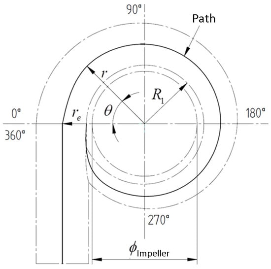
Figure 1.
Trajectory of the spiral case.
The radial distance r can be expressed as:
Simplifying further:
Taking the time derivative of this expression yields the velocity components:
Since , the radial velocity simplifies to:
where is the radial velocity and is the angular velocity. The total velocity vector is then given by:
Both the radial and tangential components of the velocity are constant. The radial velocity component is determined using Torricelli’s theorem, giving:
Given the orthogonality of the velocity components, the tangential velocity component is derived from the tangent function. To calculate this, the angle , obtained from the ratio of the inlet and outlet areas of the SC, is needed. The relationship is expressed as:
The total velocity is determined using the Pythagorean theorem:
3. Flow Analysis Using Potential Flow Theory
The use of potential flow theory is based on the physical observation that, for an ideal fluid (inviscid and incompressible), the flow can be assumed to be irrotational. Under these conditions, the velocity field can be fully described by a scalar potential. This formulation directly follows from the Euler equations when viscous effects are negligible and ensures that the continuity equation (mass conservation) is automatically satisfied, provided that the scale potential is harmonic. The assumption of irrotationality implies the absence of local sources or sinks in the fluid, thereby justifying the use of a potential function to represent the flow field. Therefore, the potential flow theory is applied to validate the fluid behavior within the spiral case. The flow is considered irrotational if:
In this case, the velocity field can be expressed as the gradient of a scalar potential function :
In two dimensions, the velocity components u and v are expressed as:
For incompressible flow, the continuity equation, in terms of the potential function , becomes:
This equation indicates that defines equipotential lines, with the Laplace equation being linear. As a result, the velocity field can be superposed as:
Since spirals are conveniently represented in polar coordinates, the Laplace equation in polar form becomes:
In polar coordinates, the radial and angular velocity components are given by:
Now that we have defined the equipotential lines, it is important to introduce the concepts of streamlines, or stream functions (). Streamlines are perpendicular to the equipotential lines and are tangent to the velocity vectors. This relationship can be described by the following equation:
When the stream function is constant, its derivative is zero, which implies:
The velocity components can be related to the stream function by:
For irrotational flow from the perspective of streamlines, the vorticity must satisfy the following condition:
Furthermore, the stream function must satisfy the Laplace equation:
The relationship between the potential function and the stream function is governed by the Cauchy–Riemann conditions, which describe how these two scalar fields are orthogonal and complementary in describing the irrotational, incompressible flow. These relationships hold in Cartesian and polar coordinate systems and provide a framework to deduce the velocity field from either potential or stream functions. As previously described, these functions satisfy the Laplace equation together to define a velocity field where streamlines and equipotential lines are mutually orthogonal. This dual representation simplifies inviscid flows’ analytical treatment and numerical modeling, particularly in geometries such as spiral casings.
To avoid redundancy, the explicit forms of these expressions are not repeated here, as they are already defined in earlier equations. Instead, the reader is referred to the fundamental relations previously presented for computing velocity components in terms of either or , depending on the coordinate system used.
Once these relationships are defined, it is important to note that the flow rate between two streamlines depends on the variation of the stream function between them. The continuity equation for the flow rate is expressed as:
This can be rewritten in terms of the stream function as:
The total flow rate between two streamlines, corresponding to and , is then:
Applying to the velocity equation, we confirm the irrotationality of the flow. This yields the following:
Additionally, differentiating the radial velocity with respect to and r results in:
Thus, we can confirm that the flow is irrotational, validating the use of potential flow theory in this analysis.
These theoretical derivations are consistent with the observed streamline behavior in the numerical simulations. As shown in Section 5, the vortex-free, irrotational velocity field aligns with the predictions of potential flow theory, supporting the validity of the Archimedean design without the need for vanes.
4. Computational Model and Code Development
A computational code was developed in MATLAB R2024b to generate the curves corresponding to each cross-section based on the mathematical model described earlier. These curves were subsequently used for digital modeling and simulation in CAD software PTC CREO v11.
The coordinates of each cross-sectional curve are calculated as follows:
The output was saved in IBL (I-Basic Component Language) format, ensuring compatibility with most CAD tools.
Here, represents the angle of the arc of the cross-section, refers to the radius of the spiral at a given angle , and denotes the radius of the cross-section at the same .
A user interface was developed using the GUIDE module in MATLAB. The interface facilitates data entry, visualization, and file saving. To perform the three-dimensional modeling of the spiral case (SC), the curves generated by the computational code were imported into PTC CREO v11 software. These curves were combined using the boundary blending tool to create surfaces. Caps were then added at both the inlet and outlet of the case. Once all surfaces were constructed, they were joined to form a solid, enabling final body operations, as shown in Figure 2. The spiral case designed for this work has an inlet diameter of 75 mm and an outlet diameter of 150 mm with a height of 30 mm.
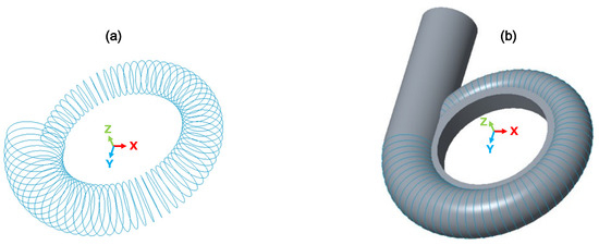
Figure 2.
Geometry generated in PTC CREO. (a) Imported curves. (b) Spiral case fluid volume.
The numerical solution for CFD problems is obtained by solving the Navier–Stokes equations with Reynolds averaging:
Mass conservation:
Momentum conservation:
Energy conservation:
where:
In the above equations, p represents pressure, is the fluid density, is the velocity vector, denotes the mass forces, represents the energy source term, is the turbulent stress tensor, h is the specific enthalpy, is the dynamic viscosity, is the thermal conductivity, and is the Kronecker delta.
4.1. Domain Discretization
A structured discretization was selected using the ICEM module of Ansys 2024R1 software to ensure accurate computational domain representation. Similar CFD studies in hydropower research, including those analyzing gravitational vortex turbines with various rotor configurations [42,43], have employed ANSYS 2024R1 CFX to evaluate performance under different flow conditions. The geometry was partitioned to achieve a higher number of control lines and ensure an accurate representation of the computational domain. The initial domain, shown in Figure 3a, was subdivided into 35 separate bodies, resulting in the configuration shown in Figure 3b. This process produced the discretized domain presented in Figure 3c.
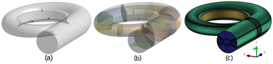
Figure 3.
Simulation domain. (a) Complete. (b) Partitioned. (c) Meshed.
To accurately capture the near-wall flow behavior, inflation layers were applied along the solid boundaries (walls of the SC) in the final mesh used for all CFD simulations. The inflation setup included 20 layers with a first layer thickness of 0.05112 mm and a growth rate of 1.1, ensuring sufficient resolution of the boundary layer without excessive element count. Including these layers significantly improves the accuracy of turbulence modeling near the wall, which is especially important when using the SST turbulence model. This refined mesh with inflation was used consistently across all simulations reported in this study.
The results of the GCI method for three different cell-count three-dimensional grids = 36,020,128 (finest grid), = 4,525,327 (medium grid), and = 71,527 (coarsest grid). The grid refinement ratios satisfy the ASME recommendation [44] regarding its lower limit value ( > 1.3) because = 1.9966 and = 3.9847. The CFD response variable was the gauge total pressure , whose numerical values, from finest to coarsest, were = 2194.25605 Pa, = 2165.8630 Pa and = 2060.80493 Pa. A monotonic convergence was achieved because the ratio of the difference between the response variables is positive ( = 3.7001) as well as the apparent order (p = 0.5747). This fact allowed the correct application of the GCI method. Finally, the mesh metrics for a mesh of 4.5 million elements reached a maximum aspect ratio of 20, while the performance of the quality and the 3 × 3 determinant exceeded the value of 0.4 for both variables.
The obtained apparent order p differs from the theoretical second-order advection scheme used in CFX (High Resolution, p = 2). This difference could be attributed to some shortcomings in the mesh quality, mesh refining, non-linearity of the solution, and turbulence modeling [45]. Despite this, these apparent orders are still acceptable for demonstrating mesh convergence [44].
The medium-to-fine and coarse-to-medium extrapolated values were both = 2252.4443 Pa. The approximate relative errors were , = 4.8506%. The extrapolated relative errors were and = 3.8439%. Moreover, the extrapolated values , give an asymptotic grid solution when h tends to zero, i.e., an infinitely refined grid. The extrapolated relative errors , compare the fine and medium grid solution concerning the extrapolated grid solution. Both the approximate and extrapolated relative errors are considered acceptable due to the low percentage error. Furthermore, the Grid Convergence Index (GCI) for the fine and medium grids were = 3.3148% and = 4.9969%, respectively. These GCI values fall within acceptable thresholds [46]. Lastly, we decided to use the medium grid because its GCI result is an acceptable value. At the same time, the cell count is maintained relatively low compared to the finest grid, allowing more efficient CFD simulations, and some previous studies of spiral chambers have employed values that are also below 5% as seen in [5].
Figure 4 shows the monotonic convergence of the response variable applying the GCI study for the three different grid cell counts , and . The y-axis is represented by the CFD response variable of gauge total pressure . The x-axis is defined by the grid cell representative size h. A value of h close to zero signifies a more refined grid. In this manner, while h tends to zero, the grid solution values tend to converge. The value corresponds to the Richardson Extrapolation when the grid size is infinitely refined, i.e., infinitely small grid cells. Finally, the characteristics grid size ranges from approximately 0.00303 to 0.02409. This allowed us to test a wide range of grid cell counts to prove the convergence of the obtained solutions.
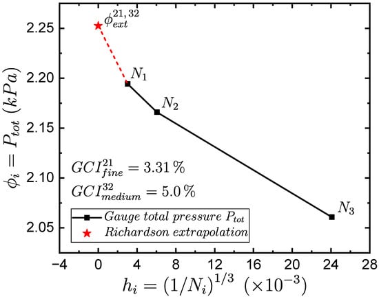
Figure 4.
Grid Converge Index (GCI) results.
4.2. Configuration of CFD Simulation
For this case, stationary single-phase simulations were conducted, with water selected as the working fluid. The SST (Shear Stress Transport) turbulence model was employed, combining the model in the central region of the domain with the model near the walls. This hybrid approach is particularly effective at capturing boundary layer phenomena, especially where flow transitions from laminar to turbulent. However, a highly refined mesh near the walls is required to resolve these transitions accurately. The SST model is generally more suited for incompressible flow, as it has limitations when applied to compressible flows. Additionally, gravity was applied along the negative Y-axis with a magnitude of 9.81 m/s2.
The boundary conditions were defined and applied to the regions shown in Figure 5, with specific values presented in Table 1. All simulations were carried out using the CFX module in Ansys software. Where the Reynolds number changes as a function of the inlet velocity and the values are 74,850, 112,275, and 149,700, for the cases of 1 m/s, 1.5 m/s, and 2 m/s, respectively.
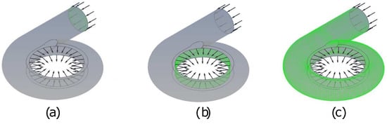
Figure 5.
Boundary conditions. (a) Inlet. (b) Opening. (c) Walls.

Table 1.
Boundary conditions.
The mesh independence study, which included fifteen analysis points, required 120 computational hours, with individual processing times ranging from 2 h to 9.7 h. The study also allowed for determining the standard deviation of the final results. The fluid dynamics simulations themselves required an additional 86 computational hours to complete.
The simulations performed range from 1 to 2 m/s, with a step of 0.5 m/s, in which the tangential and normal velocity of the fluid are measured at four angles of the exit periphery of the SC those angles are 0°, 90°, 180° and 270°. For each of these angles, the measurement is made at the central height of the SC exit which means that the Pitot tube was positioned 15 mm from the upper and lower surfaces of the SC exit region.
4.3. Experimental Setup
For the experimental setup, the model of the fiberglass spiral case was initially built. The components’ description is shown in Table 2, following the hydraulic and instrumentation diagram in Figure 6.
Table 2.
Components used in the experimental setup.
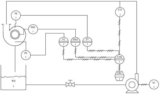
Figure 6.
Hydraulic and instrumentation diagram. Where WS is the water supply or iso tank, SC the speed controller, FIT the flow indicator transmitter, PE the primary pressure element, PDE primary differential pressure element (Pitot Tube), PT the pressure transmitter, PDIT the differential pressure indicator transmitter, UTR the multi-variable transmitter recorder (Data Acquisition System), and URC the multi-variable recorder controller (PC).
The complete experimental setup is shown in Figure 7, illustrating all the components used. Figure 8 shows the spatial positioning of the Pitot Tube in the exit region of the Spiral Case. In this figure, it is also possible to appreciate in detail the total and static pressure ports used by the Pitot tube to determine the flow velocities with differential pressure analysis.
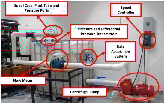
Figure 7.
Experimental setup.
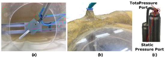
Figure 8.
Pitot Tube spatial positioning in the exit region of the Spiral Case. (a) Angular position control. (b) Vertical positioning control. (c) Total and Static pressure ports.
The direct differential pressure provided by the Pitot Tube and indirect velocity measurements were performed manually, positioning the Pitot Tube. While the total pressure port of the Pitot tube was aligned with the outflow velocity, which was corroborated by pressure measurements, since the highest total pressure level of the Pitot tube corresponds to the case where the pressure port is aligned with the outflow. This procedure was performed by changing the positioning angle of the Pitot tube by 90 degrees (0°, 90°, 180°, and 270°) to perform the measurements of the total and normal velocity components at the whole outlet region of the spiral case. The above, while the flow conditions were controlled using the variable speed drive of the centrifugal pump by regulating the frequency delivered by it, according to the flow reading provided by the flow meter, to obtain the inlet velocities of the fluid previously simulated. In addition, an experimental pressure measurement was also performed on the meridional plane of the spiral case at the angular positions of 0°, 90°, 180°, and 270° as was also proposed previously by [35]. These data were compared with those obtained numerically, as reported in the following section, to take into account the fundamental variables of this type of device, which are flow velocity and pressure.
5. Analysis of Numerical and Experimental Results
To analyze the fluid dynamic behavior of the spiral case, Figure 9a shows the velocity contour in the southern plane of the spiral case so that according to the color scale shown in the legend on the left side, the velocity of the different regions can be identified, which reaches a maximum value of 4.056 m/s in the exit region (202.8% of the inlet velocity). Such velocity behavior occurs because as the fluid moves through the spiral case, it experiences a progressive decrease in flow area, leading to a redistribution of the velocity components. The reduction of the flow cross-sectional area in the outlet region relative to the flow volume results in an increase in velocity in such a way as to comply with the mass conservation principle. This effect is a direct consequence of the geometrical properties of the Archimedes spiral, where the variation of the cross-sectional area of the spiral case promotes a nearly uniform velocity distribution in the meridional plane. Furthermore, the potential flow theory predicts fluid acceleration without significant rotational effects, which is corroborated by numerical and experimental results. The velocity vectors are also presented, allowing one to qualitatively identify a vortex free flow, validating the potential flow theory previously presented.
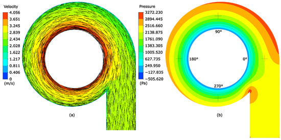
Figure 9.
Numerical results for 2 m/s inlet velocity. (a) Velocity vectors and contour. (b) Pressure contour.
The numerical velocity vectors shown in Figure 9a confirm the irrotational and vortex-free nature of the flow, as expected from the potential flow model. The smooth distribution of velocity magnitudes and directions, particularly at the outlet region, validates the flow mechanism proposed in Section 3 and demonstrates that the Archimedean geometry alone is sufficient to maintain uniform flow.
In the meridional plane, the velocity tends to be constant. A behavior similar to that achieved by [47] who, without using guide vanes, could obtain an output velocity of 187.5% of the input velocity. Or the results of [48] who reached in the output region 199.8% of the input speed, but using guide vanes. Although both authors did not develop an experimental analysis. Pressure contours shown in Figure 9b make physical sense since the highest pressures are found near the outer walls of the spiral case, in the region between 0° and 90°, since this is where the initial fluid directional change occurs, while the lowest magnitudes are associated with the outlet region, since there the fluid loses its confinement. These results agree with the work of [47,48]. On the other hand Ummar [32], also achieved numerical behaviors similar to those shown in Figure 9. However, when considering the experimental performance, the results obtained do not specifically present the performance of the spiral case, and they do not take into account the pressure heads in the turbomachine. The experimental results of the output velocity are divided into the total, radial, and tangential components, where each one of them is shown in Figure 10, Figure 11 and Figure 12, respectively, where the three input velocities analyzed are considered, and the numerical results obtained previously are added to facilitate the understanding of the numerical-experimental validation.
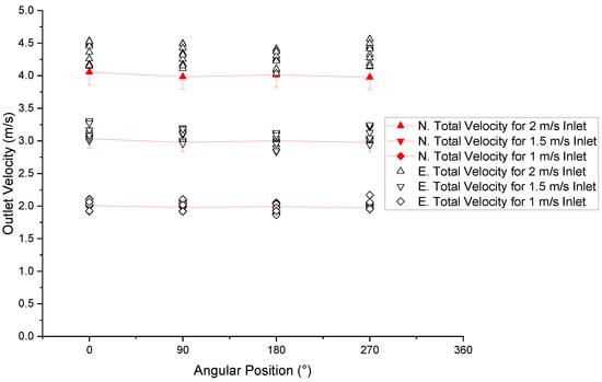
Figure 10.
Comparison of numerical and experimental results of total output velocity vs. angular position.
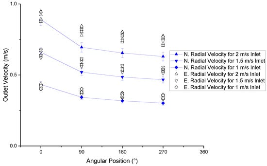
Figure 11.
Comparison of numerical and experimental results of radial output velocity vs. angular position.
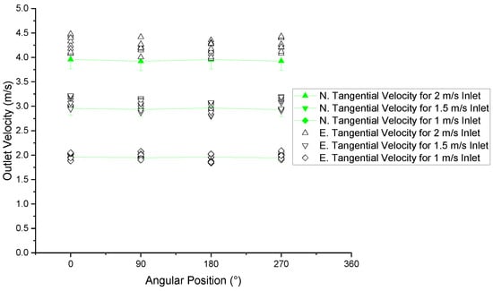
Figure 12.
Comparison of numerical and experimental results of tangential output velocity vs. angular position.
Analyzing Figure 10, it is possible to appreciate how, with the increase of the input speed, the error percentages between the numerical and experimental data of the total output speed also increase, with an average value of 3.859%, where the maximum error percentage is 8.497%, while the minimum is 0.512%. The experimental total velocity tends to be slightly higher than the numerical results, likely due to localized disturbances introduced by the Pitot Tube. Because this device, in turn, generates a partial reduction of the outlet area, which by mass conservation principle leads to an increase in velocity, which is more significant at the specific point of measurement, since it is where the flow is disturbed.
On the other hand, the analysis of the radial component of the velocity presented in Figure 11 shows a greater range of percentage error between the numerical and experimental data ranging from 15.166% to 1.494% with an average value of 9.995%. This is attributed to the difficulty of accurately capturing the radial flow using a Pitot tube aligned in multiple angular directions. On the other hand, as the radial component of the velocity is the one with the smallest magnitudes, it ends up being the most affected at the time of experimental measurements by the sensitivity of the measuring instruments.
Finally, when the tangential component of the velocity is analyzed using Figure 12, error percentages between 8.284% and 0.835% are found, with an average value of 3.824%. All of the above allows us to identify a high-reliability index of the results obtained since in these analyses it was found that for the average mesh, the error of the numerical data is 4.98%, and to this must be added the uncertainty associated with the measurement instruments previously reported in Table 2. For this reason, Table 3 is presented, where it is possible to appreciate the deviation of the velocity measurements taken in the exit region of the spiral case as a function of the input velocities evaluated. It should be noted that these experimental data correspond to those presented in Figure 10, Figure 11 and Figure 12. Table 3 is divided into the total, radial and tangential components of the velocity. Finally, by means of the last row, the percentage of error between the average values measured and their respective standard deviation was reported for the different conditions evaluated, reaching a maximum value of 3.94% and a minimum of 2.47% values consistent with those previously reported in Table 2.
Table 3.
Uncertainty of the velocity measurements made.
Table 4 shows how the numerical and experimental pressures decrease with decreasing inlet velocity, which is expected behavior if the principle of energy conservation is considered, since higher flow rates imply higher amounts of energy, behavior which in turn is confirmed by the reduction of the deviation of the experimental pressure results reported therein. The pressure distribution follows an expected decreasing trend as the fluid moves through the spiral case, consistent with the energy conservation principle. Higher pressures are observed near the inlet (0° position) due to the confined flow, while lower pressures are recorded at 270° due to expansion and flow acceleration towards the outlet.
Table 4.
Pressure analysis.
This trend is not only consistent across all three inlet velocities (1.0, 1.5, and 2.0 m/s), but also reflects the role of the Archimedean spiral geometry in gradually reducing the flow passage area, which facilitates the redistribution of pressure energy into kinetic energy. The pressure reduction observed across angular positions illustrates the conversion of hydraulic potential into motion, in accordance with Bernoulli’s equation for incompressible flow.
Moreover, the experimental data show that as the inlet velocity increases, the standard deviation in pressure measurements also increases—most notably at 180° and 270°—suggesting that higher velocities amplify localized flow instabilities or turbulence. This is consistent with the expectation that increased flow energy may cause more pronounced oscillations or deviations near the walls, particularly in regions of rapid expansion. Conversely, lower inlet velocities result in smoother pressure profiles and reduced deviation, indicating more stable flow conditions that align closely with the ideal assumptions of potential flow theory.
The discrepancies between numerical and experimental results, particularly at 180° and 270°, are primarily attributed to localized flow disturbances and the limitations of the Pitot tube placement in capturing exact static pressure variations. This is compounded by the finite resolution of the pressure sensors and the limited number of sampling points, which may not fully capture spatial gradients in rapidly evolving regions of the flow. Additionally, slight misalignments in the experimental setup or surface imperfections in the fabricated spiral case may cause localized deviation from theoretical predictions.
The average error of 11.089% is within an acceptable range for CFD-experiment comparison in similar studies [49]. In particular, for a complex geometry with three-dimensional flow features and without the aid of guide vanes to stabilize the incoming streamlines, such an error level is indicative of a strong correlation between simulated and observed behavior. The pressure fluctuations observed between 90° and 180° suggest slight variations in flow alignment within the case, which can be attributed to the geometric shrinkage of the Archimedean spiral. This geometric transition inherently alters the local curvature and sectional area, producing localized accelerations and decelerations that influence the pressure field. The numerical model is sensitive to these transitions, and the consistency of the pressure pattern with the theoretical expectations validates the capability of the CFD setup to capture flow evolution within this non-conventional configuration.
This behavior supports the theoretical predictions made in Section 3 regarding potential flow characteristics, confirming that the vaneless design maintains a stable pressure gradient throughout the system. Taken together, the findings in Table 4 underscore the potential of the Archimedean spiral casing to ensure smooth pressure reduction and energy conversion without relying on internal guide vanes—supporting its suitability for practical hydraulic applications that seek simpler and lower-maintenance geometries.
Another point to be considered in the analysis of the numerical and experimental results is the performance of the velocity measurements through a Pitot tube, because this device generates an obstruction to the flow in the exit region of the spiral case, which is why, for future work, it is recommended the incorporation of the PIV technique (Particle Image Velocimetry). Because this technique is not intrusive and it is likely that the results obtained are closer to the experimental ones.
6. Conclusions
This study presents a mathematical, numerical, and experimental analysis of a vaneless spiral case based on the Archimedean spiral, aiming to simplify the design while maintaining acceptable fluid dynamic performance. The numerical model, developed using potential flow theory and validated through CFD simulations, shows good agreement with the experimental results, with average velocity and pressure errors of 5.893% and 11.089%, respectively. The proposed design achieves a uniform velocity distribution at the outlet, with a velocity increase of up to 202.8% relative to the inlet. Although the current study does not include a complete numerical comparison with spiral cases that incorporate guide vanes, available literature suggests that similar designs with guide vanes report comparable outlet velocity gains, ranging between 187.5% and 199.8% of the inlet velocity. These results indicate that the proposed vaneless configuration can achieve competitive performance in fluid acceleration while offering significant simplification in geometry and internal flow management. By eliminating guide vanes, the proposed design reduces the number of internal components, which directly translates into lower manufacturing complexity, simplified maintenance procedures, and potentially lower operational costs. Although a detailed economic analysis is beyond this study’s scope, removing vane assemblies is expected to reduce fabrication time and misalignment-related maintenance issues, particularly in small to medium hydropower installations where cost sensitivity is high. These trade-offs support the claim that the performance of the vaneless spiral case is acceptable within its intended application context. However, it is important to acknowledge the assumptions and simplifications made in this study. The mathematical formulation assumes incompressible, inviscid, and irrotational flow based on potential flow theory, which excludes viscous effects and turbulence-driven phenomena. The CFD simulations use steady-state conditions and the SST turbulence model and do not account for surface roughness, structural deformation, or operational transients. These factors may influence the accuracy of the results in full-scale or highly turbulent environments. As such, while the current model effectively captures the primary flow behavior and provides valuable insight for design purposes, its generalizability to all operational scenarios is limited. Future research should focus on optimizing the spiral geometry to enhance flow uniformity, incorporating more advanced turbulence models such as LES or RSM to capture finer-scale effects, and validating the design across a broader range of operating conditions. A follow-up study should consider a detailed cost-performance analysis comparing vane and vaneless designs. Additionally, investigating the long-term structural behavior and cavitation risk in full-scale implementations will be crucial for assessing practical deployment. These efforts will support the advancement of efficient and accessible hydropower solutions and expand the applicability of simplified hydraulic designs.
Author Contributions
Conceptualization, D.H.Z.; Methodology, S.V.-G. and D.H.Z.; Software, S.V.-G.; Validation, S.V.-G. and O.D.M.-C.; Formal analysis, S.V.-G. and D.S.-V.; Investigation, D.S.-V.; Resources, D.H.Z.; Data curation, O.D.M.-C. and D.H.Z.; Writing—original draft, S.V.-G. and O.D.M.-C.; Writing—review & editing, D.S.-V.; Visualization, O.D.M.-C. and D.S.-V.; Supervision, D.H.Z. and D.S.-V. All authors have read and agreed to the published version of the manuscript.
Funding
This research received no external funding.
Data Availability Statement
The original contributions presented in the study are included in the article; further inquiries can be directed to the corresponding author.
Acknowledgments
The authors would like to express their gratitude for the support received from all academic institutions, as well as for the project P21104 (Fortalecimiento del grupo MATyER) at the Instituto Tecnológico Metropolitano. During the preparation of this work, the authors used Grammarly 1.112.1.0 and ChatGPT 4o to improve their writing and style. After using this tool, the authors reviewed and edited the content as needed and took full responsibility for the publication’s content.
Conflicts of Interest
The authors declare no conflicts of interest.
References
- Ardizzon, G.; Cavazzini, G.; Pavesi, G. A new generation of small hydro and pumped-hydro power plants: Advances and future challenges. Renew. Sustain. Energy Rev. 2014, 31, 746–761. [Google Scholar] [CrossRef]
- UPME. Plan de Expansión de Referencia Generación-Transmisión 2015–2029; Ministerio Minas y Energía: Bogotá, Colombia, 2016; 616p.
- Trivedi, C.; Cervantes, M.J.; Gandhi, B.K.; Ole, D.G. Experimental investigations of transient pressure variations in a high head model Francis turbine during start-up and shutdown. J. Hydrodyn. 2014, 26, 277–290. [Google Scholar] [CrossRef]
- Cervantes, M.J.; Sundström, J.; Shiraghaee, S.; Kjeldsen, M.; Wiborg, E.J. Extending the operational range of Francis turbines: A case study of a 200 MW prototype. Energy Convers. Manag. X 2024, 23, 100681. [Google Scholar] [CrossRef]
- Danieli, P.; Masi, M.; Lazzaretto, A.; Carraro, G. An engineering approach for the fast simulation of radial inflow turbines with vaneless spiral casing by single-channel CFD models. In An Engineering Approach for the Fast Simulation of Radial Inflow Turbines with Vaneless Spiral Casing by Single-Channel CFD Models; EDP Sciences: Les Ulis, France, 2021; Volume 312. [Google Scholar]
- Chen, X.; Lai, X.; Gou, Q.; Song, D. Effect of guide vane profile on the hydraulic performance of moderate low-specific-speed Francis turbine. J. Mech. Sci. Technol. 2023, 37, 1289–1300. [Google Scholar] [CrossRef]
- Yi, Y.; Wang, W.; Li, T.; Gao, Z.; Lu, L.; He, L. Optimization design and test verification of guide vanes for a fish-friendly Francis turbine. J. Phys. Conf. Ser. 2024, 2752, 012012. [Google Scholar] [CrossRef]
- Favre, L.; Chiarelli, M.; El Hayek, N.; Niederhüuser, E.L.; Donato, L. Design and performance evaluation of a substitution solution for spiral casing of pico-hydroelectric plants. IOP Conf. Ser. Earth Environ. Sci. 2019, 240, 042018. [Google Scholar] [CrossRef]
- Ghimire, A.; Dahal, D.; Kayastha, A.; Chitrakar, S.; Thapa, B.S.; Neopane, H.P. Design of Francis turbine for micro hydropower applications. J. Phys. Conf. Ser. 2020, 1608, 012019. [Google Scholar] [CrossRef]
- Koirala, R.; Neopane, H.P.; Shrestha, O.; Zhu, B.; Thapa, B. Selection of guide vane profile for erosion handling in Francis turbines. Renew. Energy 2017, 112, 328–336. [Google Scholar] [CrossRef]
- Joy, J.; Raisee, M.; Cervantes, M.J. A novel guide vane system design to mitigate rotating vortex rope in high head Francis model turbine. Int. J. Fluid Mach. Syst. 2022, 15, 188–209. [Google Scholar] [CrossRef]
- Koirala, R.; Thapa, B.; Neopane, H.P.; Zhu, B. A review on flow and sediment erosion in guide vanes of Francis turbines. Renew. Sustain. Energy Rev. 2017, 75, 1054–1065. [Google Scholar] [CrossRef]
- Cui, G.; Cao, Y.; Yan, Y.; Wang, W. Numerical study on high-fidelity flow field around vanes of a Francis turbine. Phys. Fluids 2024, 36, 045137. [Google Scholar] [CrossRef]
- Leguizamon-Perilla, A.; Rodriguez-Bernal, J.S.; Moralez-Cruz, L.; Farfán-Martinez, N.I.; Nieto-Londoño, C.; Vásquez, R.E.; Escudero-Atehortua, A. Digitalisation and modernisation of hydropower operating facilities to support the Colombian energy mix flexibility. Energies 2023, 16, 3161. [Google Scholar] [CrossRef]
- Paniagua-García, E.; Perafán-López, J.C.; Nieto-Londoño, C.; Vásquez, R.E.; Sierra-Pérez, J.; Taborda, E. Hydrokinetic resource assessment in Colombia’s Non-Interconnected Zones: Case study. Int. J. Thermofluids 2024, 22, 100675. [Google Scholar] [CrossRef]
- Davies, L.; Saygin, D. Distributed Renewable Energy in Colombia: Unlocking Private Investment for Non-Interconnected Zones; Organisation for Economic Co-Operation and Development—OECD: Paris, France, 2023. [Google Scholar] [CrossRef]
- Keck, H.; Sick, M. Thirty years of numerical flow simulation in hydraulic turbomachines. Acta Mech. 2008, 201, 211–229. [Google Scholar] [CrossRef]
- Keck, H.; Hass, W. Vorticity and blade circulation modeling in the calculation of quasi-three-dimensional cascade flows with finite elements. In Proceedings of the 3rd International Conference on Finite Elements in Flow Problems, Banff, AB, Canada, 10–13 June 1980. [Google Scholar]
- Tiwari, G.; Kumar, J.; Prasad, V.; Patel, V.K. Multi-fidelity CFD for obtaining the runner blade profile parameters of a Francis turbine for optimum hydrodynamic performance. Ocean Eng. 2024, 305, 117994. [Google Scholar] [CrossRef]
- Altintas, B.; Ayli, E.; Celebioglu, K.; Aradag, S.; Tascioglu, Y. Mitigating cavitation effects on Francis turbine performance: A two-phase flow analysis. Ocean Eng. 2025, 317, 120018. [Google Scholar] [CrossRef]
- Göde, E.; Cuénod, R.; Pestalozzi, J. Visualization of flow phenomena in a hydraulic turbine based on 3D flow computations. In Proceedings of the International Conference on Hydropower (Waterpower’89), Niagara Falls, NY, USA, 23–25 August 1989; ASCE: New York, NY, USA, 1989; pp. 1802–1811. [Google Scholar]
- Huang, X.; Ou, H.; Huang, H.; Wang, Z.; Wang, G. Flow-Induced Stress Analysis of a Large Francis Turbine Under Different Loads in a Wide Operation Range. Appl. Sci. 2024, 14, 11782. [Google Scholar] [CrossRef]
- Wang, J.; Liu, J.; Lu, Y.; Li, H.; Zhang, X. Machine learning-driven high-fidelity ensemble surrogate modeling of Francis turbine unit based on data-model interactive simulation. Eng. Appl. Artif. Intell. 2024, 133, 108385. [Google Scholar] [CrossRef]
- Masoodi, F.; Goyal, R. Simulation and validation of a Francis turbine load rejection procedure using OpenFOAM CFD code. IOP Conf. Ser. Earth Environ. Sci. 2024, 1411, 012064. [Google Scholar] [CrossRef]
- Pochylỳ, F.; Haluza, M.; Veselỳ, J. The Francis Pump Turbine With Stochastic Blades. Procedia Eng. 2012, 39, 68–75. [Google Scholar] [CrossRef]
- Fu, X.; Li, D.; Wang, H.; Zhang, G.; Li, Z.; Wei, X. Influence of the clearance flow on the load rejection process in a pump-turbine. Renew. Energy 2018, 127, 310–321. [Google Scholar] [CrossRef]
- Rezavand Hesari, A.; Gauthier, M.; Coulaud, M.; Maciel, Y.; Houde, S. Flow characteristics of a Francis turbine under deep part-load and various no-load conditions. Exp. Fluids 2024, 65, 166. [Google Scholar] [CrossRef]
- Zhang, S.; Zhang, X.; Luo, Y.; Gao, T.; Wang, Z. Preloading Clearance Effects on Hydrodynamic Characteristics of Preloading Spiral Case and Concrete in Pump Mode. Water 2024, 16, 3122. [Google Scholar] [CrossRef]
- Xiao, Y.x.; Wang, Z.w.; Zhang, J.; Luo, Y.y. Numerical predictions of pressure pulses in a Francis pump turbine with misaligned guide vanes. J. Hydrodyn. 2014, 26, 250–256. [Google Scholar] [CrossRef]
- Yan, X.; Kan, K.; Zheng, Y.; Chen, H.; Binama, M. Entropy Production Evaluation within a Prototype Pump-Turbine Operated in Pump Mode for a Wide Range of Flow Conditions. Processes 2022, 10, 2058. [Google Scholar] [CrossRef]
- Zhao, W.; Deng, J.; Jin, Z.; Xia, M.; Wang, G.; Wang, Z. A Comparative Analysis on the Vibrational Behavior of Two Low-Head Francis Turbine Units with Similar Design. Water 2025, 17, 113. [Google Scholar] [CrossRef]
- Umar, B.M.; Cao, J.; Wang, Z. Experimental and Cfd Simulation Validation Performance Analysis of Francis Turbine. IOP Conf. Ser. Earth Environ. Sci. 2022, 1037, 012003. [Google Scholar] [CrossRef]
- Liu, P.; Huang, X.; Yang, T.; Wang, Z. Flow-Induced Fatigue Damage of Large Francis Turbines Under Multiple Operating Loads. Appl. Sci. 2024, 14, 12003. [Google Scholar] [CrossRef]
- Ma, Y.; Pang, X.; Wang, Z.; Huang, D.; Liu, X.; Zeng, Y.; Yao, B.; Pang, J.; Gang, Y.; Hu, Y.; et al. Design and Validation of a Testing Device for Sediment-Induced Erosion Based on Similarity Theory. Water 2025, 17, 222. [Google Scholar] [CrossRef]
- Shrestha, U.; Choi, Y.D. Improvement of flow behavior in the spiral casing of Francis hydro turbine model by shape optimization. J. Mech. Sci. Technol. 2020, 34, 3647–3656. [Google Scholar] [CrossRef]
- Danieli, P.; Masi, M. Adaption of the single-channel approach to use the CFD code MULTALL as an effective tool in the preliminary design of radial inflow turbines with vaneless spiral casing. In Proceedings of the 15th European Conference on Turbomachinery Fluid Dynamics & Thermodynamics, Budapest, Hungary, 24–28 April 2023. [Google Scholar]
- Fuller, A.M.; Alexander, K.V. Exit-flow velocity survey of two single-tangential-inlet vaneless turbine volutes. Exp. Therm. Fluid Sci. 2011, 35, 48–59. [Google Scholar] [CrossRef]
- Pan, L.; Yang, M.; Murae, S.; Sato, W.; Kawakubo, T.; Yamagata, A.; Deng, K. Study on aerodynamic excitation of radial turbine blades with vaneless volute at low excitation order. J. Fluids Struct. 2021, 107, 103408. [Google Scholar] [CrossRef]
- Wang, L.; Wei, D. The optimum structural design for spiral case in hydraulic turbine. Procedia Eng. 2011, 15, 4874–4879. [Google Scholar] [CrossRef]
- Stojkovski, F.; Lazarevikj, M.; Markov, Z.; Iliev, I.; Dahlhaug, O.G. Constraints of parametrically defined guide vanes for a high-head francis turbine. Energies 2021, 14, 2667. [Google Scholar] [CrossRef]
- Liang, A.; Li, H.; Zhang, W.; Yao, Z.; Zhu, B.; Wang, F. Study on pressure fluctuation and rotating stall characteristics in the vaneless space of a pump-turbine in pump mode. J. Energy Storage 2024, 94, 112385. [Google Scholar] [CrossRef]
- Del Rio, J.A.S.; Sánchez, A.R.; Villa, D.S.; Quintana, E.C. Numerical Study of H-Darrieus Turbine as a Rotor for Gravitational Vortex Turbine. CFD Lett. 2022, 14, 1–11. [Google Scholar] [CrossRef]
- Sánchez, A.R.; Del Rio, J.A.S.; Quintana, E.C.; Sanín-Villa, D. Numerical comparison of Savonius turbine as a rotor for gravitational vortex turbine with standard rotor. J. Appl. Eng. Sci. 2023, 21, 204–211. [Google Scholar]
- Celik, I.B.; Ghia, U.; Roache, P.J.; Freitas, C.J. Procedure for estimation and reporting of uncertainty due to discretization in CFD applications. J. Fluids Eng.-Trans. ASME 2008, 130, 078001. [Google Scholar]
- Slater, J.W. Examining Spatial (Grid) Convergence. 2019. Available online: http://www.grc.nasa.gov/www/wind/valid/tutorial/spatconv.html (accessed on 12 December 2024).
- Almohammadi, K.; Ingham, D.; Ma, L.; Pourkashan, M. Computational fluid dynamics (CFD) mesh independency techniques for a straight blade vertical axis wind turbine. Energy 2013, 58, 483–493. [Google Scholar] [CrossRef]
- Gizem, O. Utilization of CFD Tools in the Design Process of a Francis Turbine. Ph.D. Thesis, Middle East Technical University, Ankara, Turkey, 2010. [Google Scholar]
- Augustson, T.M. Flow Conditions in Spiral Casing and the Influence of Various Bend Geometries. Master’s Thesis, Institutt for Energi- og Prosessteknikk, Trondheim, Norway, 2013. [Google Scholar]
- Trivedi, C.; Cervantes, M.J.; Dahlhaug, O.G. Experimental and numerical studies of a high-head Francis turbine: A review of the Francis-99 test case. Energies 2016, 9, 74. [Google Scholar] [CrossRef]
Disclaimer/Publisher’s Note: The statements, opinions and data contained in all publications are solely those of the individual author(s) and contributor(s) and not of MDPI and/or the editor(s). MDPI and/or the editor(s) disclaim responsibility for any injury to people or property resulting from any ideas, methods, instructions or products referred to in the content. |
© 2025 by the authors. Licensee MDPI, Basel, Switzerland. This article is an open access article distributed under the terms and conditions of the Creative Commons Attribution (CC BY) license (https://creativecommons.org/licenses/by/4.0/).