
Set-Valued Approximation—Revisited and Improved

Abstract
1. Introduction
- For , the boundaries of are surfaces in . We remark that the case has many practical applications as it amounts to reproducing a 3D object (the graph of F) from its parallel 2D cross-sections (the samples of F). A variety of methods devised for this case are in [1,5,6,7]. None of these methods claim an approximation error higher than .
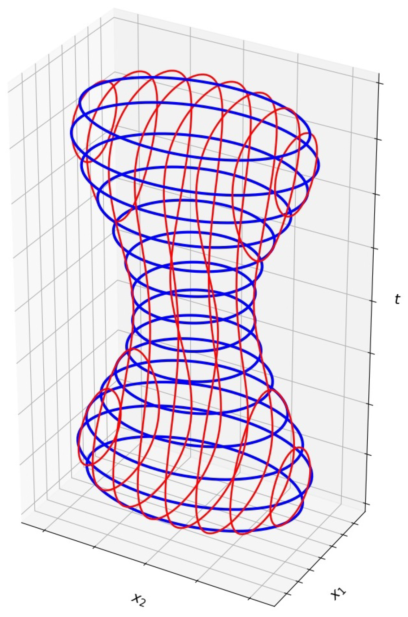
- For , the boundaries of the graph of F are 3D manifolds in , which are complicated to imagine. On the other hand, the evolution of F as a function of t is a familiar entity, which is the animation of the changing 3D sets in between the given sets. At each animation frame, we display the 2D boundary of the approximated 3D object . Based upon the method in [1], an efficient algorithm for solving this problem is presented in [2].
2. Preliminaries
2.1. Review of Multidimensional Reconstruction by Set-Valued Approximations
2.2. Approximating Piecewise-Smooth Functions
2.3. Spline Quasi-Interpolation Operators
3. Improving the DFI Method
3.1. The Signed-Distance Function
3.2. High-Order Approximation of Singular Signed-Distance Functions
- 1.
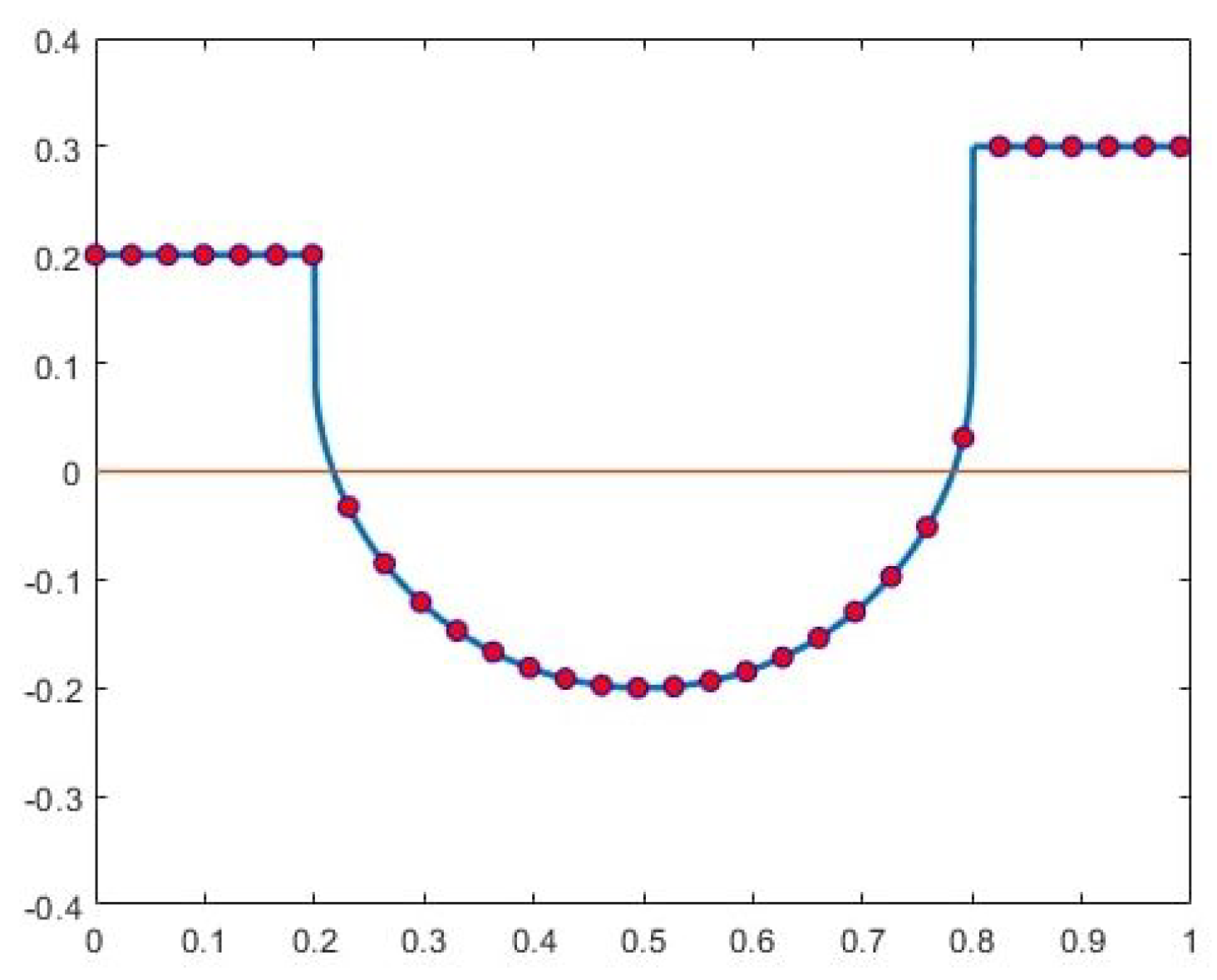
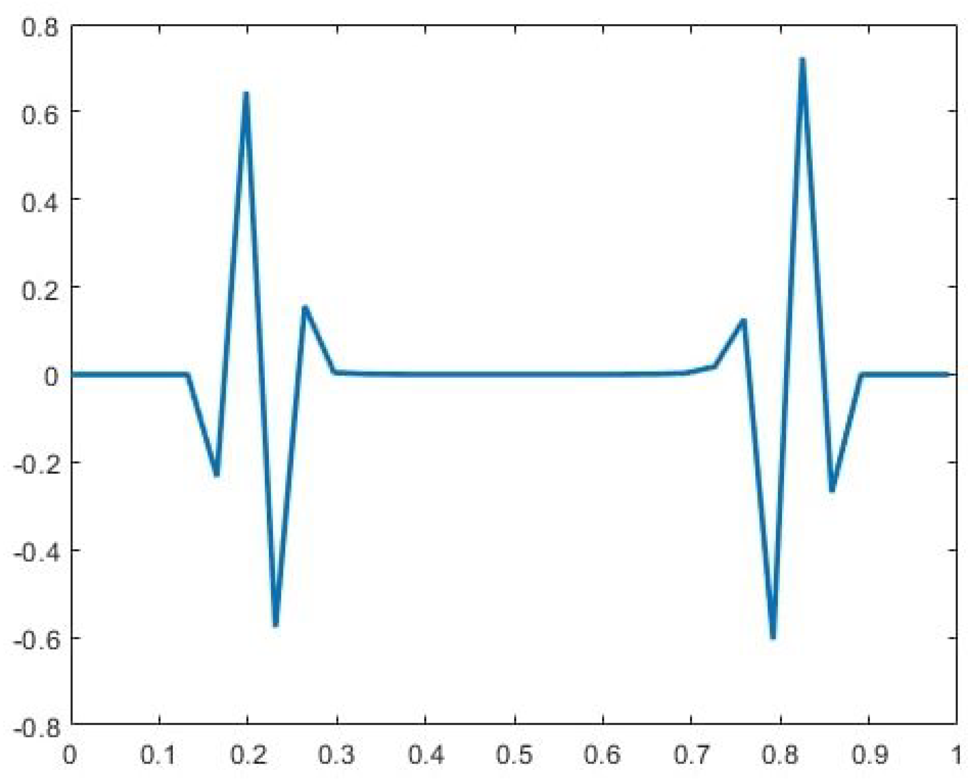
- Deriving the signature of the singularitiesWe begin by applying a p-degree quasi-interpolation operator (see Section 2.3) to the given data (represented by the circles in Figure 3). To facilitate this process, we extend the values to the left and right by padding with zero values.Next, we compute the errors in the quasi-interpolation approximation at the given data points:We recall that the quasi-interpolation operator is a local operator, utilizing only a finite number of data points for each t. It provides an approximation order to functions. Consequently, the errors remain small at points where the signed-distance function is smooth but become significantly larger near the singular points and . Additionally, large errors appear near the boundary points and . For our application, we focus on the neighborhood of the singular points and disregard the large errors near the boundaries. We refer to the values as ‘the signature of ’. For instance, the signature of the function in Figure 3 (with ) is illustrated in Figure 4.
- 2.
- Using the signature to identify singularity parametersThe next step, following [13], is to identify a singular function whose signature closely matches that of . As observed in Figure 4, for sufficiently small h, the effects of different singularities are well separated and can be analyzed independently.In our case, while the exact locations of the singularities are unknown, their type is known. To address the left singularity in the given example, we fit a singular function of the formThe unknown singularity location s along with the unknown coefficients are determined by performing minimization of the difference between the signature of and , i.e.,where the indices and specify the interval of high signature corresponding to the left singularity. The operator computes the error of the quasi-interpolation approximation at . The parameter q is chosen as to achieve the highest possible approximation order. We denote the resulting optimal parameters as , .As proved in [13], the resulting singularity parameters approximate the exact singularity parameters with a high order of accuracy. In particular, the singularity location satisfies as .
- 3.
- The ‘corrected approximation’ framework.We can now construct the desired approximation of with the above singularity information. This process is performed locally, relying upon the locality property of the quasi-interpolation operator .First, we apply to the smoothed data , whereThis yields the smooth-part approximation . Following [13], the final approximation is obtained by correcting the smooth-part approximation by reintroducing the singular component:Using the error estimates from [13], we obtain
- 4.
- Computational aspectsThe optimization problem in (10) is linear in the unknown coefficients but non-linear in the singularity location s. However, since is an approximation of one of the values where a tangent plane is tangent to , and given that there are only a finite number of such values, much of the computational effort involved in solving the nonlinear problem can be reduced. Specifically, once is well approximated for a particular point , the same approximation can be used for all points in a neighborhood of , significantly reducing the need for repeated nonlinear optimization.In general, the singularity exponent is also unknown. However, the assumption that is smooth implies that, in non-degenerate cases, the singularity exponent is expected to be . Nevertheless, other possible exponents, such as and , should also be considered.Remark 2(Approximating the tangency point ). The parameters obtained in the approximation can also be utilized to derive an estimate of the tangency point . Specifically, the value serves as an approximation of the distance between and . Additionally, recall that computing each distance involves determining the direction to the nearest point on the boundary. Let be the direction associated with , where is the closest point to s satisfying . Then, the approximation of is given byWhile the approximation achieves approximation order , the approximation of is of order .
3.3. The Improved DFI Approximation
4. Building Implicit Approximation of
4.1. Implicit Approximation of Smooth Curves and Hypersurfaces
4.2. Estimating the Distance of a Point from a Hypersurface
4.3. Distributing Points near
4.4. Completion of near Tangency Points
- In the first approach, according to Theorem 2, the approximation order is , where k is the smoothness index of the boundary.
- For the second approach, where is the degree of the polynomial used for the local approximation.
4.5. Building and Analyzing the Implicit Function Approximation
5. Summary
Funding
Data Availability Statement
Conflicts of Interest
References
- Levin, D. Multidimensional reconstruction by set-valued approximations. IMA J. Numer. Anal. 1986, 6, 173–184. [Google Scholar] [CrossRef]
- Cohen-Or, D.; Solomovic, A.; Levin, D. Three-dimensional distance field metamorphosis. ACM Trans. Graph. (TOG) 1998, 17, 116–141. [Google Scholar] [CrossRef]
- Dyn, N.; Levin, D.; Muzaffar, Q. Interpolation of set-valued functions. IMA J. Numer. Anal. 2024, drae031. [Google Scholar] [CrossRef]
- Dyn, N.; Farkhi, E.; Mokhov, A. Approximation of Set-Valued Functions: Adaptation of Classical Approximation Operators; Imperial College Press: London, UK, 2014. [Google Scholar]
- Barequet, G.; Shapiro, D.; Tal, A. Multilevel sensitive reconstruction of polyhedral surfaces from parallel slices. Vis. Comput. 2000, 16, 116–133. [Google Scholar] [CrossRef]
- Kels, S.; Dyn, N. Reconstruction of 3D objects from 2D cross-sections with the 4-point subdivision scheme adapted to sets. Comput. Graph. 2011, 35, 741–746. [Google Scholar] [CrossRef]
- Schumaker, L.L. Reconstruction of 3-D objects using splines. In Proceedings of the Curves and Surfaces in Computer Vision and Graphics, Santa Clara, CA, USA, 13–15 February 1990; Volume 1251. [Google Scholar]
- Dyn, N.; Levin, D. Approximation of Set-Valued Functions with images sets in Rd. arXiv 2025, arXiv:2501.14591. [Google Scholar]
- Amat, S.; Levin, D.; Ruiz-Alvárez, J.; Yáñez, D.F. Global and explicit approximation of piecewise-smooth two-dimensional functions from cell-average data. IMA J. Numer. Anal. 2023, 43, 2299–2319. [Google Scholar] [CrossRef]
- Amat, S.; Levin, D.; Ruiz-Álvarez, J. A two-stage approximation strategy for piecewise smooth functions in two and three dimensions. IMA J. Numer. Anal. 2022, 42, 3330–3359. [Google Scholar] [CrossRef]
- Levin, D. The approximation power of moving least-squares. Math. Comput. 1998, 67, 1517–1531. [Google Scholar] [CrossRef]
- Levin, D. Mesh-independent surface interpolation. In Geometric Modeling for Scientific Visualization; Springer: Berlin/Heidelberg, Germany, 2004. [Google Scholar]
- Lipman, Y.; Levin, D. Approximating piecewise-smooth functions. IMA J. Numer. Anal. 2010, 30, 1159–1183. [Google Scholar]
- Sober, B.; Levin, D. Manifold approximation by moving least-squares projection (MMLS). Constr. Approx. 2020, 52, 433–478. [Google Scholar]
- Dyn, N.; Farkhi, E.; Mokhov, A. Approximations of set-valued functions by metric linear operators. Constr. Approx. 2007, 25, 193–209. [Google Scholar] [CrossRef]
- Speleers, H. Hierarchical spline spaces: Quasi-interpolants and local approximation estimates. Adv. Comput. Math. 2017, 43, 235–255. [Google Scholar] [CrossRef]

Disclaimer/Publisher’s Note: The statements, opinions and data contained in all publications are solely those of the individual author(s) and contributor(s) and not of MDPI and/or the editor(s). MDPI and/or the editor(s) disclaim responsibility for any injury to people or property resulting from any ideas, methods, instructions or products referred to in the content. |
© 2025 by the author. Licensee MDPI, Basel, Switzerland. This article is an open access article distributed under the terms and conditions of the Creative Commons Attribution (CC BY) license (https://creativecommons.org/licenses/by/4.0/).
Share and Cite
Levin, D. Set-Valued Approximation—Revisited and Improved. Mathematics 2025, 13, 1194. https://doi.org/10.3390/math13071194
Levin D. Set-Valued Approximation—Revisited and Improved. Mathematics. 2025; 13(7):1194. https://doi.org/10.3390/math13071194
Chicago/Turabian StyleLevin, David. 2025. "Set-Valued Approximation—Revisited and Improved" Mathematics 13, no. 7: 1194. https://doi.org/10.3390/math13071194
APA StyleLevin, D. (2025). Set-Valued Approximation—Revisited and Improved. Mathematics, 13(7), 1194. https://doi.org/10.3390/math13071194