I-NeRV: A Single-Network Implicit Neural Representation for Efficient Video Inpainting

Abstract

Deep learning methods based on implicit neural representations offer an efficient and automated solution for video inpainting by leveraging the inherent characteristics of video data. However, the limited size of the video embedding (e.g., $16\times 2\times 4$) generated by the encoder restricts the available feature information for the decoder, which, in turn, constrains the model’s representational capacity and degrades inpainting performance. While implicit neural representations have shown promise for video inpainting, most of the existing research still revolves around image inpainting and does not fully account for the spatiotemporal continuity and relationships present in videos. This gap highlights the need for more advanced techniques capable of capturing and exploiting the spatiotemporal dynamics of video data to further improve inpainting results. To address this issue, we introduce I-NeRV, the first implicit neural-representation-based design specifically tailored for video inpainting. By embedding spatial features and modeling the spatiotemporal continuity between frames, I-NeRV significantly enhances inpainting performance, especially for videos with missing regions. To further boost the quality of inpainting, we propose an adaptive embedding size design and a weighted loss function. We also explore strategies for balancing model size and computational efficiency, such as fine-tuning the embedding size and customizing convolution kernels to accommodate various resource constraints. Extensive experiments on benchmark datasets demonstrate that our approach substantially outperforms state-of-the-art methods in video inpainting, achieving an average of 3.47 PSNR improvement in quality metrics.

1. Introduction

Video quality is a critical factor in providing a positive user experience, and any form of video corruption can significantly undermine perceived quality. Traditional video inpainting techniques, which frequently depend on complex algorithms and extensive manual interventions, can be inefficient and time-consuming. In contrast, deep-learning-based video inpainting offers a more automated and effective approach. Specifically, the implicit neural representation method treats the video as a neural network, enabling it to recover the original content from a corrupted version by automatically learning and inpainting based on extracted features. Moreover, utilizing large datasets for training further improves both accuracy and efficacy. As neural network modeling continues to advance, security considerations have received growing attention [1,2,3,4], with privacy-preserving methods and blockchain applications emerging as promising solutions for safeguarding video data. Additionally, implicit neural representation has attracted considerable interest for applications such as video compression [5,6,7], video reconstruction [8,9,10,11,12], and video synthesis [13,14,15,16].

The implicit neural representation NeRV [17] has drawn considerable attention for its compact network structure and efficient video processing capabilities, positioning it as one of the key frameworks in this rapidly evolving domain. In particular, researchers have leveraged NeRV’s versatile architecture to tackle challenging tasks where both speed and accuracy are paramount. Subsequent works, such as [15,17,18], have introduced refinements at various stages—including input design, encoder architecture, and decoder modifications—achieving notable performance gains in applications ranging from denoising to style transfer. Notably, HNeRV [19] excels in video compression by employing a highly compact embedding $(16\times 2\times 4)$. While this design significantly reduces the model size and is well-suited for compression tasks, the limited embedding scale constrains the feature capacity and ultimately impairs performance in more fine-grained tasks like video inpainting. In general, for a fixed network depth, larger embeddings carry richer feature information, which makes them more suitable for capturing detailed spatial and temporal structures crucial for high-quality inpainting.

Motivated by these insights, we propose the I-NeRV model, an image-level video neural representation framework specifically tailored for inpainting. Our experiments reveal that an embedding size of $(16\times 8\times 16)$ strikes an optimal balance between model complexity and performance, effectively capturing the necessary information for robust inpainting without excessively increasing computational overhead. To accommodate this larger embedding, we adjust the decoder structure so that deeper layers can efficiently process and reconstruct masked or corrupted regions. Additionally, we incorporate a random masking (RM) mechanism to partially occlude input video frames before they are fed into the encoder, compelling the network to learn more generalized representations and improving its resilience to diverse corruption patterns. Through extensive experiments on benchmark video datasets, we demonstrate that I-NeRV achieves state-of-the-art(SOTA) performance, reporting a remarkable $\mathbf{3}.\mathbf{47}$ peak signal-to-noise ratio(PSNR) improvement in video inpainting tasks over the previous leading methods.

• We develop a video neural representation network (I-NeRV) that performs efficient and automated video inpainting, surpassing SOTA methods and improving PSNR by $\mathbf{3}.\mathbf{47}$ on benchmark tasks.
• We propose a suitably large embedding scale and adapt decoder features accordingly, enabling richer feature information to be passed to the decoder and significantly enhancing inpainting effectiveness.
• We integrate a random mask mechanism into the encoder, wherein video frames are partially occluded before encoding. This design further improves feature extraction and makes the network robust to complex corruption patterns.

2. Related Work

2.1. Implicit Neural Representation of Video

Implicit neural representation is a novel signal representation method that approximates a mapping function by fitting a neural network. It has a strong modeling ability for different signals and is widely used in many video downstream tasks. In the early research into implicit neural representation of video, the pixels of video frames were usually encoded and decoded, which is called pixel-level coding and decoding neural networks. It trains the model to learn the mapping relationship [20,21] between the left side of a point and RGB of that point; this method has high training cost and slow coding and decoding speed. Chen et al. [17] put forward the neural representations for videos (NeRV) used to encode the indexes of video frames, which uses convolution and pixel shuffle to train the video and fit it into a neural network. This image-level neural representation greatly improves the encoding and decoding speed of the video. However, the above improvements are all based on position coding, and the correlation between the encoded embedding and the image content is weak. Therefore, Chen et al. proposed a content-adaptive encoder CNeRV [22], and the encoded embedding is content-related. Then, the author put forward another codec architecture, HNeRV [19], using the ConvNeXt [23] block to encode at the encoder end, which reduces the size of the encoded embedding and improves the video compression rate. It performs well for video compression. However, the small size of embedding limits the amount of feature information it carries and affects the effect of video inpainting. Kwan et al. [24] put forward HiNeRV in the pursuit of ultimate bit rate performance, which is the most competitive INR method in the field of video compression. However, its decoding method based on bilinear interpolation has bad performance in the field of video inpainting and video frame interpolation. In order to improve the effect of video inpainting, this paper designs a large-scale embedding to solve the problem of the lack of feature information, starting with the small-scale embedding of HNeRV.

2.2. Video Inpainting

For the task of video inpainting, many scholars have also conducted research from the perspective of pipelines or frameworks, for example, ProPainter proposed by Zhou et al. [25], AVID proposed by Zhang et al. [26], etc. All the above video inpainting methods require complex pipelines. In contrast, implicit neural representation only needs to train a neural network. This network maps the video content into points in high-dimensional space using an encoder and then reconstructs the video through a decoder. This method is simple and efficient and shows great potential in the field of video painting. Based on this, this paper constructs a network of implicit neural representations of video with a random mask, which includes a random mask module and an encoder subnet. After the video is input, it is processed by the random mask module and then enters the encoder subnet. Random masks can improve the ability of feature extraction. The encoder subnet is obtained by expanding the embedding scale of HNeRV and adjusting the feature scale of each layer of the encoder. The experiments show that I-NeRV in this paper uses a single network to improve the effect of video inpainting, avoid complex pipeline processing, simplify video inpainting, and improve the efficiency and performance of video inpainting.

3. Our Proposed Design

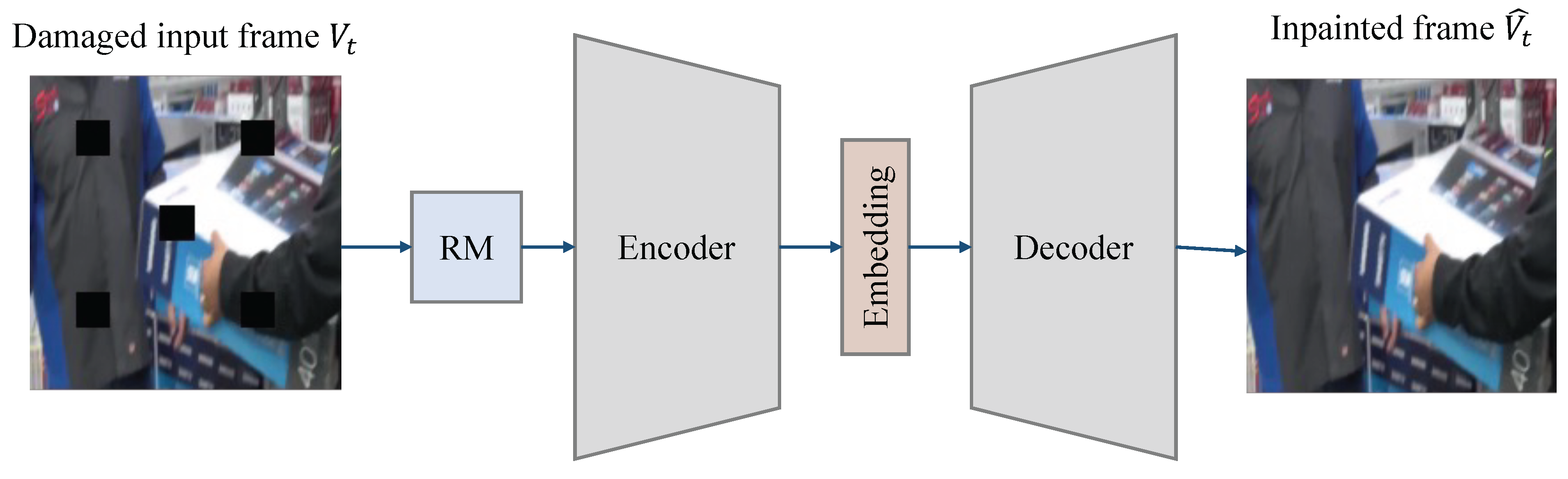
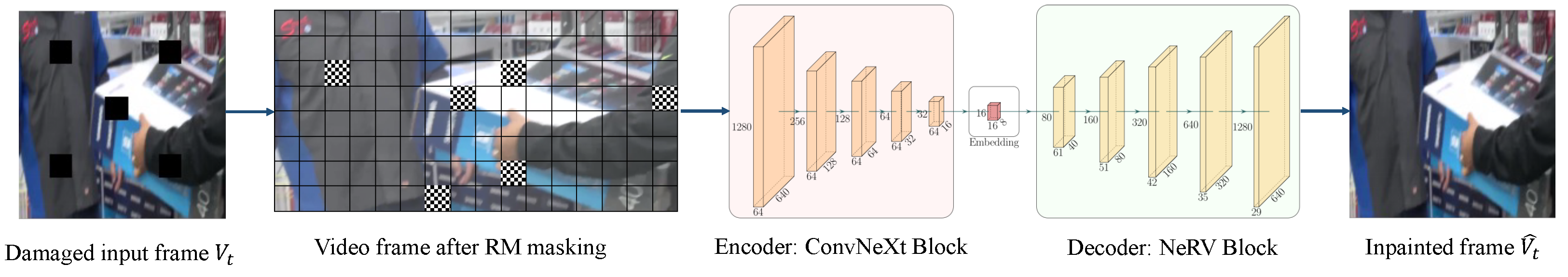
3.1. The Overall Architecture

As shown in Figure 1, our I-NeRV framework comprises a RM module and an encoder–decoder sub-network, where the encoder–decoder sub-network includes an encoder, an embedding layer, and a decoder. The input to the network is a video frame (potentially corrupted), and the output is the inpainted version of that frame. Specifically, during training, each video frame $v_t$ first passes through the RM module, which introduces partial occlusion into the input. This forces the model to learn more generalized representations, thereby improving the robustness and feature extraction capabilities. Subsequently, the masked frame is fed into the encoder, generating a feature vector (the embedding), which is then decoded to produce the inpainted frame $\widehat{v}t$. The training objective minimizes the difference between $\widehat{v}t$ and $v_t$, guiding the network to fill in missing regions more effectively.

In this process, the video as a whole is represented by the learned embeddings, and the decoder reconstructs the inpainted video from these embeddings. Of particular note, we adopt a significantly larger embedding scale ($16\times 8\times 16$) compared to the prior designs, retaining richer spatial and temporal details. While this expansion effectively enhances inpainting quality, it also necessitates structural adaptations in the decoder to handle the increased feature information more efficiently. For further clarity on the RM mechanism and the expanded embedding structure, we provide a detailed illustration in Figure 2.

3.2. Random Mask Module

The RM module divides the input video frame into N squares and then randomly selects n grids for masking (occlusion). Specifically, the input video frame is divided into N grids according to pixels, and then n grids are selected by using a random function, as shown in Equations  (1) and (2).

$$\mathrm{N}={\displaystyle \frac{\mathrm{H}\ast \mathrm{W}}{{\mathrm{a}}^2}}a\in (0,min(\mathrm{H},\mathrm{W}))$$

(1)

$$X_i=Random(\mathrm{N},\mathrm{n})i\in (1,2,\dots ,\mathrm{n})$$

(2)

In Equation (1), a is the side length of the grid, which is expressed by the number of pixels, and its value range is 0 and the minimum value of pixel height and width, and H and W are the height and width of pixels of the input video frame, respectively. In Equation (2), $X_i$ is one of the n grids randomly selected, the range of i is from 1 to n, and Random is a random function that can be selected as required or designed by yourself. Here, the most common random function is selected.

The video frames are randomly masked using six masks with side lengths of 80. The RM module masks the input video frame $v_t$ after dividing it into a number of grids of equal side lengths. The model will be forced to learn the spatial layout and pixel-to-pixel correspondence of the display of the video frame $v_t$, instead of understanding the video frame $v_t$ only as a vector representation lacking spatial dimensionality. Furthermore, unlike simply collapsing video frame $v_t$ into vectors, due to the continuity of the sequence of video frames passing through the $\mathrm{RM}$ module, the model will learn this continuity relationship between pixels.

3.3. Encoder Sub-Network

When the video is inpainted by using the implicit neural representation of the video, the features of the encoded $v_t$ video frame by the encoder are used as embedding, and an appropriate size is designed for embedding. Therefore, the embedding carries more feature information, to improve the effect of video inpainting. With the change in embedding size, the feature size of the encoder in the network needs to be adjusted accordingly, and the network scale should be balanced; that is, the scale of embedding and decoder should not be too large. Therefore, while changing the embedding size, it is required to coordinate the feature size of the decoder.

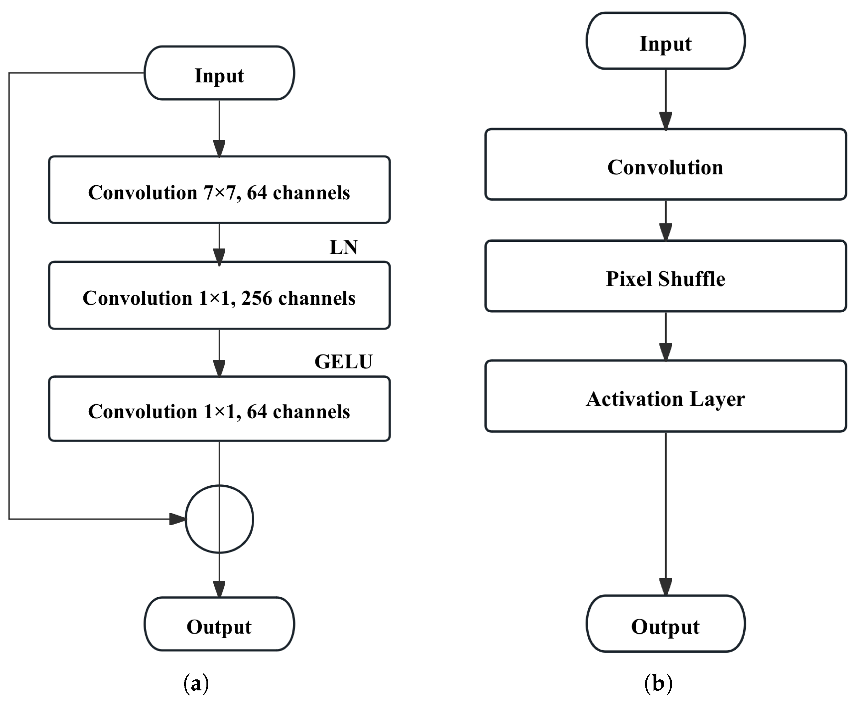
3.3.1. Encoder

The encoder uses the HNeRV structure for reference and adopts five coding layers, each of which contains a ConvNeXt [23] block, and  $v_t$ down-samples the video input frame 5 times. Each video input frame $v_t$ corresponds to an $f_t$ embedding. The structure of the ConvNeXt block is as shown in Figure 3a. After the first four down-samplings, the number of channels is increased to 64 after one $7\times 7$ convolution each time, and then layer normalization (LN) is conducted. The number of channels is then increased to four times after one $1\times 1$ convolution, and the number of channels is fixed at 64 after being activated by the Gaussian error linear unit (GELU) function and one $1\times 1$ convolution. It is worth noting that in the fifth sampling, the number of channels of the three convolutions is set to 16, 64, and 16 in order to obtain a more reasonable embedding size.

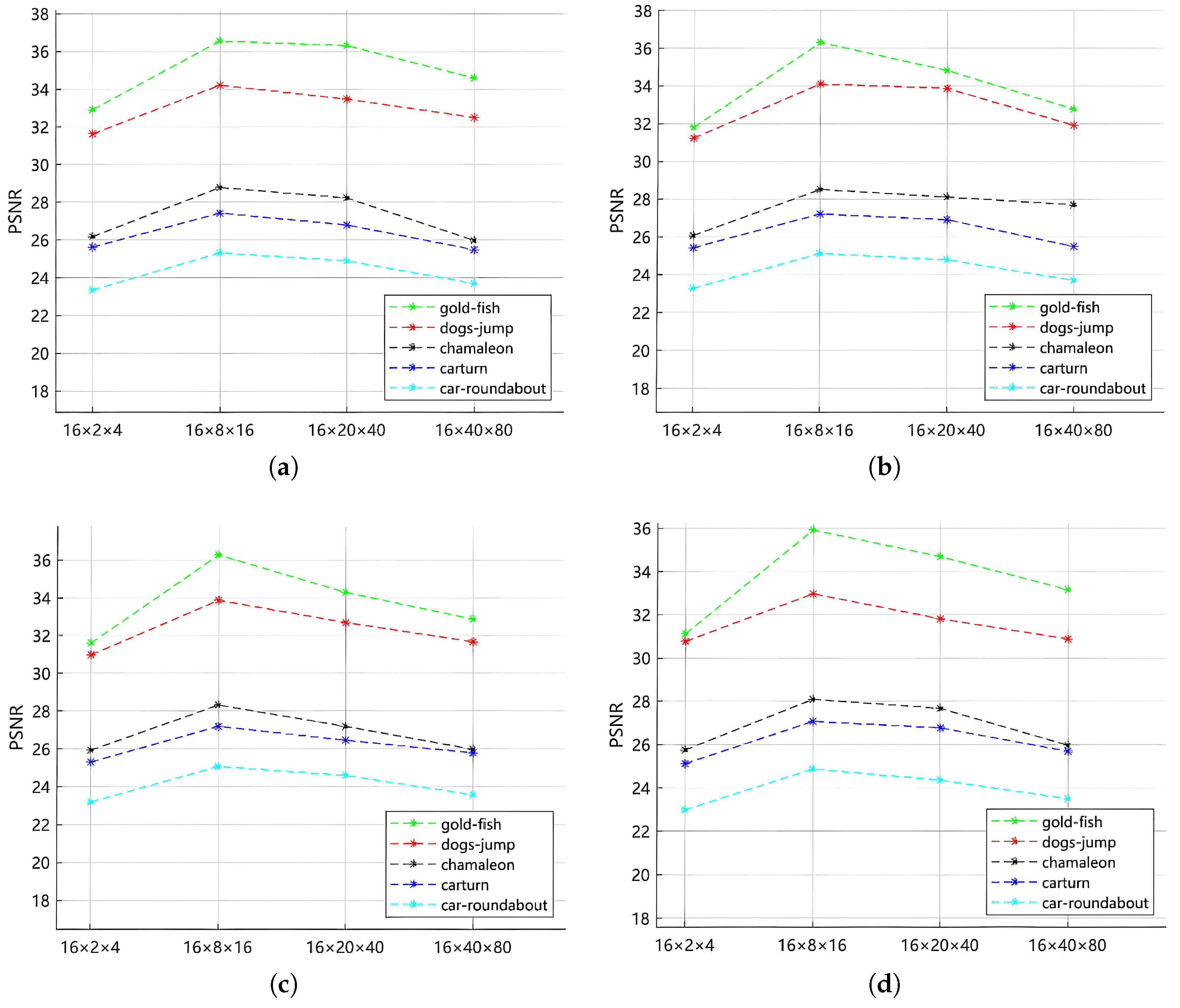
3.3.2. Embedding Size Design

Increasing the embedding size provides a straightforward method to enhance the feature representation capacity of the network. However, it is essential to balance the need for rich information flow with the risk of model redundancy. We systematically investigated several commonly used embedding sizes in neural video representation, including $16\times 2\times 4$, $16\times 8\times 16$, $16\times 20\times 40$, and $16\times 40\times 80$, while maintaining a fixed total model size of 1.5 million parameters. To ensure fair comparisons, we adjusted the convolution kernel sizes in the decoder accordingly. These kernel sizes were selected from the set $\{1, 3, 5, 7\}$ and applied in various sequences, allowing each embedding configuration to stay within the same parameter budget.

Performance was primarily evaluated using PSNR, which is a key metric in assessing video inpainting quality. As reported in

Table 1. PSNR values of 16 combinations of convolution kernel and embedding sizes.

Convolution Kernel Size	Embedding Size	PSNR
$\{1, 3, 3, 3, 3\}$	$16\times 2\times 4$	27.404
	$16\times 8\times 16$	30.144
	$16\times 20\times 40$	29.046
	$16\times 40\times 80$	27.962
$\{1, 5, 3, 3, 3\}$	$16\times 2\times 4$	27.94
	$16\times 8\times 16$	30.458
	$16\times 20\times 40$	29.942
	$16\times 40\times 80$	28.452
$\{1, 5, 5, 3, 3\}$	$16\times 2\times 4$	27.566
	$16\times 8\times 16$	30.25
	$16\times 20\times 40$	29.7
	$16\times 40\times 80$	28.292
$\{1, 7, 5, 3, 3\}$	$16\times 2\times 4$	27.15
	$16\times 8\times 16$	29.784
	$16\times 20\times 40$	29.06
	$16\times 40\times 80$	27.84

and Figure 4, the embedding configuration of $16\times 8\times 16$ combined with decoder kernel sizes of $1, 5, 3, 3, 3$ consistently delivered the best PSNR results across five benchmark video datasets. In practice, this kernel combination effectively captures both coarse structures and fine-grained details, while the selected embedding size provides a receptive field large enough to handle diverse motion patterns and texture variations. Although larger embeddings such as $16\times 20\times 40$ marginally increased feature richness, they offered limited performance improvement and introduced unnecessary redundancy. On the other hand, smaller embeddings like $16\times 2\times 4$ lacked the capacity to fully capture the spatiotemporal complexity of the input.

Taking these observations into account, we adopted the embedding size of $16\times 8\times 16$ along with decoder kernel sizes of $1, 5, 3, 3, 3$ in the final design. This configuration strikes an effective balance between representation power and computational efficiency, enabling robust video inpainting performance. Nevertheless, the findings also indicate that alternative combinations of embeddings and kernel sizes may be better suited for specific tasks, and future implementations can benefit from further exploration of these design choices.

3.3.3. Decoder

The decoder end consists of five decoding layers, and each decoding layer contains a NeRV block, which consists of a convolution layer, a pixel shuffle layer, and an activation layer, respectively. The structure of the NeRV block is shown in Figure 3b. Among them, the convolution layer mainly learns the parameters in the process of output frame ${\widehat{v}}_t$ reconstruction, and its channel number decreases proportionally, which is an important part of implicit neural representation. The pixel shuffle layer splices the parameters after convolution to carry out up-sampling, improve the vector size, and gradually reach the required resolution. An activation function is placed in the activation layer, and ReLU is used as the activation function in this paper. The embedding is decoded by the decoder and then output through the activation layer.

3.4. Loss Function

In network training, the loss function is very important and directly affects the effect of video inpainting. When selecting the loss function, it is required to weigh the advantages and disadvantages of different functions and consider the characteristics of specific application scenarios. For example, in real-time video communication, we may pay more attention to calculation speed, while in high-quality film production, we may pay more attention to image quality. We will pay more attention to the size of the video in video compression tasks and pay attention to the quality of the video itself in video inpainting and video frame interpolation tasks. In this paper, the mean squared error (MSE) loss function is adopted, as shown in Equation (3).

$$\mathrm{MSE}={\displaystyle \frac{1}{n}}\sum _{i=1}^n{\left({\widehat{Y}}_i-Y_i\right)}^2$$

(3)

MSE is the most intuitive loss function, which punishes the error by calculating the square of the difference between the predicted value ${\widehat{Y}}_i$ and the actual value $Y_i$. This square operation magnifies the influence of large errors, so the model will pay special attention to reducing these large prediction errors. MSE is the first choice in many optimization problems because its mathematical properties usually make the solution process simpler.

Unlike MSE, L1 loss gives equal weight to both small and large errors. It will not excessively punish large errors, which is particularly useful when dealing with outliers. L1 loss is often used to generate sparsity, for example, in feature selection or compressive sensing, as shown in Equation  (4).

$$\mathrm{L}1=\sum _{\mathrm{i}=1}^{\mathrm{n}}\left|{\widehat{\mathrm{Y}}}_{\mathrm{i}}-{\mathrm{Y}}_{\mathrm{i}}\right|$$

(4)

Structural similarity index measure (SSIM) is an evaluation indicator of video, and it can also be used as a loss function. It considers both the difference in pixel values and the structural information of images. SSIM assesses the change in image quality by simulating the working principle of the human visual system. See Equation (5) for details.

$$SSIM(\mathrm{x},\mathrm{y})={\displaystyle \frac{\left(2{\mu }_{\mathrm{x}}{\mu }_{\mathrm{y}}+{\mathrm{C}}_1\right)\left(2{\sigma }_{\mathrm{xy}}+{\mathrm{C}}_2\right)}{\left({\mu }_{\mathrm{x}}^2+{\mu }_{\mathrm{y}}^2+{\mathrm{C}}_1\right)\left({\sigma }_{\mathrm{x}}^2+{{\sigma }_{\mathrm{y}}}^2+C_2\right)}}$$

(5)

${\mu }_{\mathrm{x}}$ and ${\mu }_{\mathrm{y}}$ are the average brightness of images $\mathrm{X}$ and $\mathrm{Y}$, ${{\sigma }_{\mathrm{x}}}^2$ and ${{\sigma }_{\mathrm{y}}}^2$ are the variance of images $\mathrm{X}$ and $\mathrm{Y},{\sigma }_{\mathrm{xy}}$ is the covariance of images $\mathrm{X}$ and $\mathrm{Y}$, and ${\mathrm{C}}_1$ and ${\mathrm{C}}_2$ are small constants added to avoid the denominator being zero.

Through a large number of experiments, this paper proves that the performance of I-NeRV can be enhanced by using the weighted loss function, so the loss function used in this paper is shown in Equation (6).

$$\mathrm{Loss}=0.3\times \mathrm{L}1+0.7\times \mathrm{SSIM}$$

(6)

3.5. I-NeRV Video Inpainting Process

I-NeRV is a deep-learning-based implicit neural representation model designed for efficient video inpainting. The proposed method utilizes an encoder–decoder structure along with a random masking mechanism to improve feature extraction and enhance inpainting robustness. The structured pipeline of I-NeRV follows Algorithm 1.

The video inpainting process begins by iterating over each input frame $v_t$ (line 3). The frame first undergoes random masking, where the input video frame is divided into equal-sized grids, and a set of n random grids are selected and masked (lines 5–7). This process enhances the model’s robustness to complex corruption patterns. Next, the masked frame $v_t^{\prime }$ is encoded (line 8). The encoder extracts multi-scale feature representations using convolutional layers. These extracted features are then transformed into an embedding $e_t$ (line 9), which serves as a compact latent representation of the input frame. The embedding is then passed through the decoder to reconstruct the missing parts of the frame (line 10). The decoder applies deconvolutional layers to gradually refine and reconstruct the inpainted frame ${\widehat{v}}_t$. The final output is stored as part of the inpainted video sequence $\widehat{V}$ (line 11). By leveraging the implicit neural representation framework, I-NeRV efficiently maps video frames to a continuous latent space, significantly improving inpainting accuracy while reducing computational complexity. The combination of random masking, encoder-based feature extraction, and decoder-based reconstruction allows I-NeRV to achieve state-of-the-art performance in video inpainting.

Algorithm 1: I-NeRV video inpainting Process

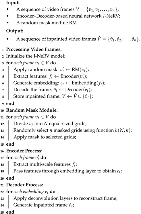4. Experiment

4.1. Experiment Data

The DAVIS [27] and UVG [28] datasets are both commonly used in the video field. However, the DAVIS dataset is more authoritative, providing over 100 dynamic and challenging video scenes. Most other video frame sequences are generally less than 100 frames long, making DAVIS more challenging for video inpainting and better for assessing the performance of video inpainting methods. However, there are only two or three hundred video frames in the UVG dataset. To better verify the efficiency of the video inpainting algorithm proposed in this paper, the DAVIS dataset was chosen. This dataset contains videos with two resolutions, 480p and 1080p, covering a variety of dynamic environments. We have selected some videos from it to ensure the coverage of different scenes from single target to multi-target complex interaction. Five data sets with 1080p resolution including gold-fish, dogs-jump, chameleon, car-turn, and car-roundabout are mainly selected. In the experiment, video frames are preprocessed into images with 640 × 1280 resolution and normalized to meet the input requirements.

4.2. Experiment Configuration

In the experiment, this paper sets the grid side length a to be 80 and the number n of randomly selected grids to be 6 in the random mask module. In the process of network training, the Adam optimizer is used, and a moderate initial learning rate of 0.001 and a dynamically adjusted learning rate attenuation mechanism are set. In addition, regularization techniques, such as weight attenuation and early stop strategy, are introduced to prevent the model from over-fitting. Two batches are processed in each training, and the model size is set to 1.5M. The coding step size of the encoder is set to $\{5, 2, 2, 2, 2\}$, and the sizes of the five-layer features after coding are 64 × 640 × 1280, 64 × 128 × 256, 64 × 64 × 128, 64 × 32 × 64, and 64 × 16 × 32, respectively. The decoding step size of the decoder is set to $\{5, 2, 2, 2, 2\}$, and the sizes of the five-layer features after decoding are 61 × 40 × 80, 51 × 80 × 160, 42 × 160 × 320, 35 × 320 × 640, and 29 × 640 × 1280, respectively.

4.3. Evaluation Indicator

PSNR is an important indicator to measure the effect of video coding and decoding, as shown in Equation (7).

$$\mathrm{PSNR}=10·{log}_{10}\left({\displaystyle \frac{{\mathrm{MAX}}^2}{\mathrm{MSE}}}\right)$$

(7)

MAX represents the maximum possible pixel value of the video, and MSE is the mean square error between the original video frame and the inpainted video frame. It assesses the loss of quality in the compression process by comparing the mean square error (MSE) between the original video frame and the inpainted video frame. The higher the PSNR, the smaller the visual difference between the inpainted video and the original video, and the closer the inpainted video is to the original video.

The multiscale structural similarity index (MSSSIM) is similar to SSIM with the addition of multiscale considerations to its base, and it evaluates the similarity of images at different resolutions. This approach is closer to the way the human visual system works, as the human eye naturally analyzes images at different scales when observing them. It is defined as in Equation (8).

$$MSSSIM(x,y)={\left[l_M(x,y)\right]}^{{\alpha }_M}\prod _{j=1}^M{\left[c_j(x,y)\right]}^{{\beta }_i}{\left[s_j(x,y)\right]}^{{\gamma }_j}$$

(8)

${\mathrm{l}}_{\mathrm{M}}$ is the luminance comparison on the largest scale M, $c_j(x,y)$ is the contrast comparison on scale j, $s_j(x,y)$ is the structural comparison on scale j, and ${\alpha }_M,{\beta }_i,{\gamma }_{\mathrm{j}}$ are the parameters used to adjust the weights of each component.

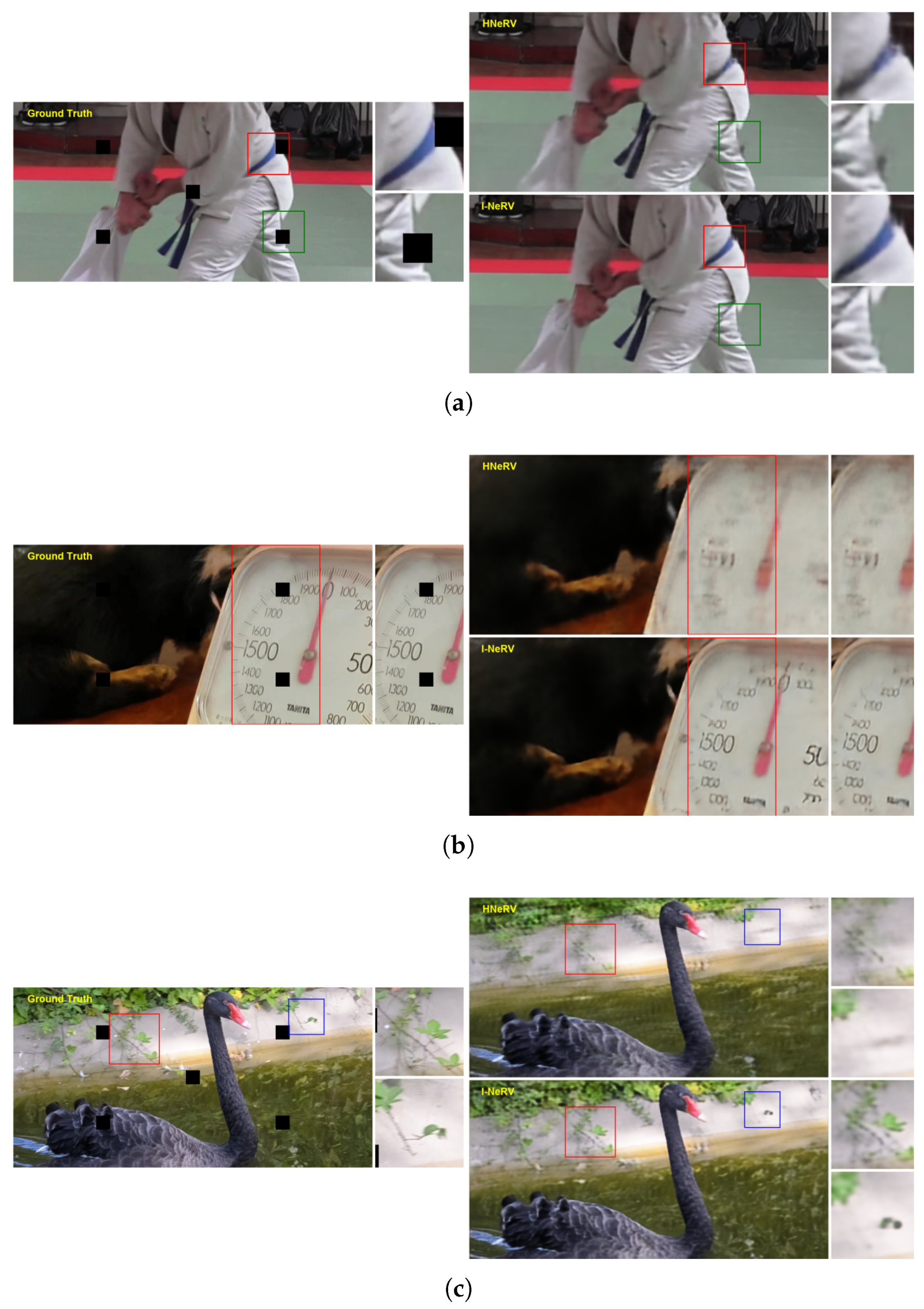
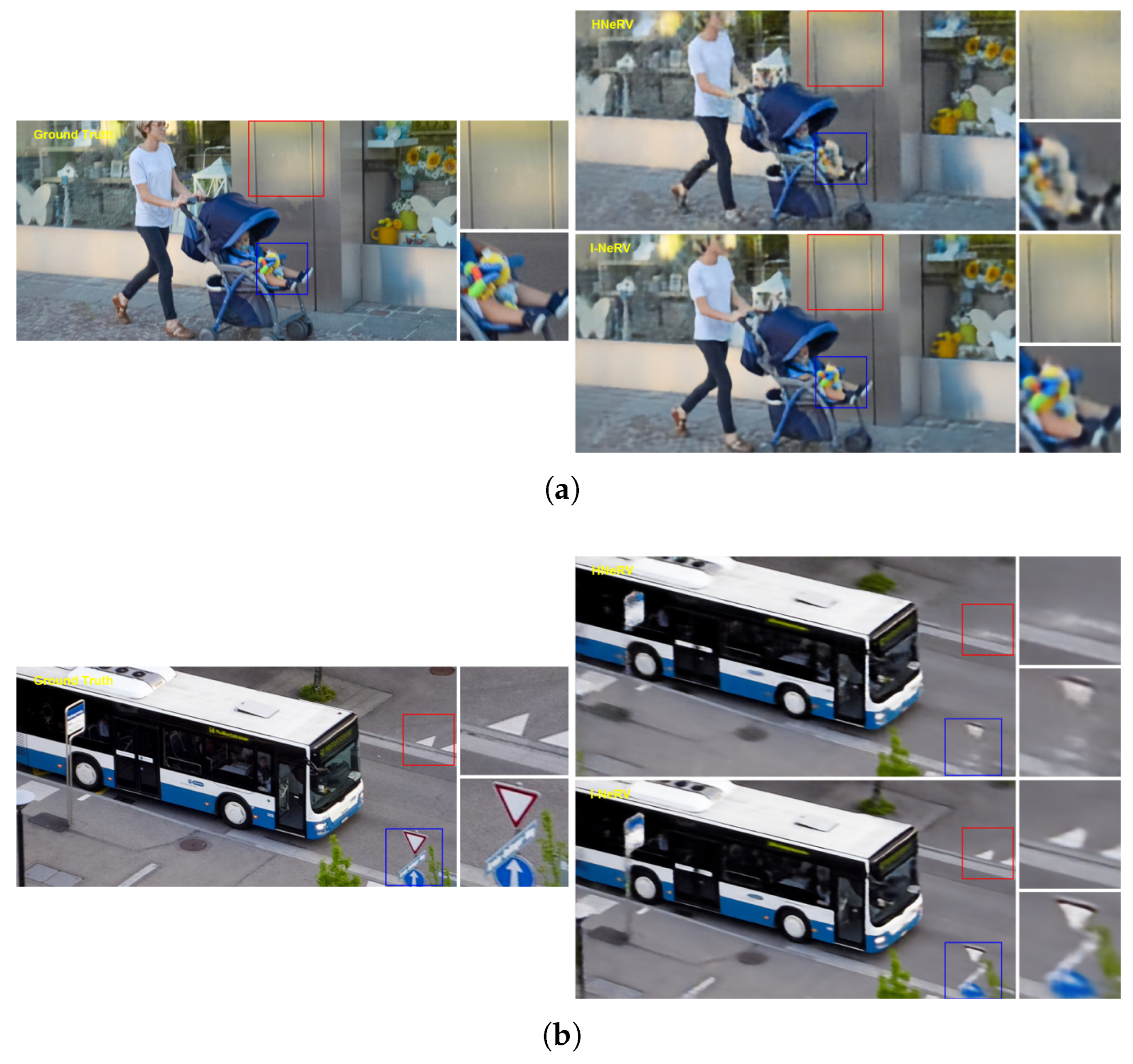
4.4. Experimental Result and Analysis

In this section, we conduct a comprehensive comparison between I-NeRV and four state-of-the-art video inpainting models: NeRV, PS-NeRV [18], HNeRV, and MNeRV [29]. To ensure a fair comparison, all models are constrained to a parameter budget of 1.5 M. The dataset images are uniformly cropped into video frames with the same resolution as the models’ input, maintaining consistent experimental settings. Figure 5 presents the evaluation results of PSNR and MSSSIM metrics across different training epochs on the judo dataset. It can be observed that I-NeRV consistently outperforms the baseline methods throughout the training process. Notably, at the early stage of training (e.g., 200 epochs), I-NeRV already surpasses all other models by a significant margin. As training progresses, the performance gap becomes more evident, particularly in MSSSIM, where I-NeRV maintains a stable advantage while other models plateau. These results highlight the superior learning efficiency and representation quality of I-NeRV under the same model capacity and data configuration. Additional quantitative results on other datasets (gold-fish, dogs-jump, chameleon, car-turn, and car-roundabout) are summarized in

Table 2. Comparative experiments on model inpainting.

Data Set	NeRV	PS-NeRV	HNeRV	MNeRV	I-NeRV
gold-fish	31.89	32.65	32.91	35.69	36.55 $(4.66\uparrow )$
dogs-jump	30.76	31.37	31.63	33.13	34.21 $(\mathbf{3}.\mathbf{45}\uparrow )$
chameleon	25.23	25.98	26.18	27.29	28.78 $(\mathbf{3}.\mathbf{55}\uparrow )$
car-turn	24.57	25.41	25.63	26.67	27.43 $(\mathbf{2}.\mathbf{86}\uparrow )$
car-roundabout	22.48	23.12	23.35	24.47	25.32 $(\mathbf{2}.\mathbf{84}\uparrow )$
		avg			$\mathbf{3}.\mathbf{47}\uparrow$

, where I-NeRV achieves an average PSNR gain of 3.47 dB and a +4.66 dB improvement on the gold-fish dataset compared to existing models.

In order to show the advantages of I-NeRV model intuitively, this paper uses I-NeRV and HNeRV to conduct comparative experiments on different data sets. For fair comparison, all models were trained for 300 rounds, and the model size was set to 3 M. In the video inpainting experiment, we selected an image from judo, dogs-scale, and blackswan for comparison before and after inpainting, and the result is shown in Figure 6. On the left is the video frame before inpainting, that is, the original image, also called Ground Truth, and the middle part shows the specific damaged parts in the original image. The upper right image shows the inpainting effect of the HNeRV model, and the lower right image shows the inpainting effect of the I-NeRV model. Among them, the part enclosed by the red frame, the green frame, or the blue frame is blurred or occluded in the original picture, and it is the effect of the corresponding part in the picture on the right. It can be clearly seen that on the judo data set, the blue belt position of the video frame is lost, and the color of HNeRV is distorted in the inpainting of this part, and I-NeRV is closer to the original picture; On the dogs-scale data set, in the video frame after HNeRV inpainting, the dial of the scale is blurred, and the numbers on the I-NeRV table are clearer; On the blackswan data set, HNeRV even has the directly missing objects, but I-NeRV does not have this problem. Three sets of pictures clearly show that I-NeRV has strong video inpainting ability. Compared with the benchmark model HNeRV, I-NeRV has obvious improvement in video inpainting and clearer effect in some details.

In addition, this paper conducts comparative experiments on the video frame interpolation performance of I-NeRV and HNeRV using the stroller and bus datasets. For fairness, both models followed the video frame interpolation processing pipeline of HNeRV. The interval frames were deleted, and the remaining video frames were trained into models to predict the intermediate interval frames, using the same parameter settings. Figure 7 shows the effect of video frame interpolation of I-NeRV and HNeRV. In the figure, the original picture is on the left, the details of the framed part are in the middle, the frame interpolation effect of HNeRV is on the upper right, and the frame interpolation effect of I-NeRV is on the lower right. By observing the red and blue frames, we can find that I-NeRV is better than HNeRV in the frame interpolation effect, which further proves that I-NeRV is also better than the baseline model HNeRV in video frame interpolation tasks.

4.5. Ablation Experiment

Random Mask Module and Embedding Ablation Experiment

Table 3. Ablation experiment of RM and embedding.

Data Set	RM Module	Embedding	HNeRV
gold-fish	×	×	$32.91/0.9293$
	√	×	$33.46/0.9431$
	√	√	36.55/0.9485
dogs-jump	×	×	31.63/0.9299
	√	×	$32.21/0.9473$
	√	√	34.21/0.9609
chameleon	×	×	26.18/0.9197
	√	×	26.84/0.9266
	√	√	28.78/0.9305
car-turn	×	×	$25.63/0.8645$
	√	×	25.97/0.8697
	√	√	27.43/0.8804
car-roundabout	×	×	$23.35/0.8771$
	√	×	$24.11/0.8826$
	√	√	25.32/0.8873

presents an ablation study designed to evaluate the individual and combined contributions of the random masking (RM) module and the enhanced embedding component to the performance of the video inpainting network. The first column lists the evaluated datasets, while the second and third columns indicate whether the RM module and embedding enhancements are included, respectively. A checkmark “√” denotes that the corresponding component is included in the model configuration, and a cross “×” indicates that it is not applied. The fourth column reports the performance of the model under each configuration using the baseline HNeRV framework, where the results are expressed in the format “PSNR/MSSSIM”. Specifically, the numerical value to the left of the slash represents the PSNR, and the value to the right corresponds to the MSSSIM.

The configuration in which both the RM module and the embedding enhancement are applied (i.e., both entries in the second and third columns are “√”) corresponds to our proposed method, I-NeRV. This full configuration consistently achieves the best performance across all datasets, as highlighted in bold in the table. These results demonstrate that both the RM module and the enhanced embedding design independently contribute to performance gains, and their combination leads to further improvements in video inpainting quality.

To determine the most suitable loss function for the model proposed in this paper, an ablation study of the loss function was conducted on the Judo dataset. This study explored the effect of different combinations of loss functions on the model’s video inpainting performance. The ablation results are shown in

Table 4. Ablation analysis of the loss function.

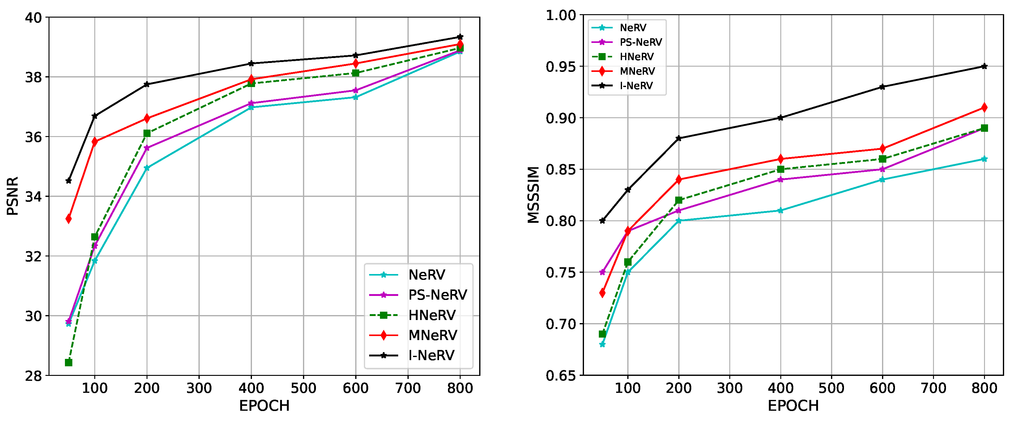
Loss Function	PSNR	MSSSIM
$\mathrm{L}1$	35.12	0.9622
$\mathrm{L}2$	34.08	0.9617
$\mathrm{SML}1$	34.08	0.9617
$0.3\times \mathrm{L}2+0.7\times \mathrm{S}$	35.66	0.9528
$0.5\times \mathrm{L}2+0.5\times \mathrm{S}$	35.49	0.9625
$0.5\times \mathrm{L}1+0.5\times \mathrm{S}$	36.64	0.9649
$0.7\times \mathrm{L}2+0.3\times \mathrm{S}$	36.17	0.9634
$0.7\times \mathrm{L}1+0.3\times \mathrm{S}$	36.33	0.9628
$0.7\times \mathrm{L}2+0.3\times \mathrm{L}1$	34.75	0.9619
$0.7\times \mathrm{L}1+0.3\times \mathrm{MS}$	36.18	0.9637
$0.3\times \mathrm{L}1+0.7\times \mathrm{MS}$	36.26	0.9639
$0.8\times \mathrm{L}1+0.2\times \mathrm{MS}$	36.07	0.9648
$0.3\times \mathrm{L}1+0.7\times \mathrm{S}$	36.67	0.9651

. Where “S” stands for the loss function for SSIM metrics, and “MS” stands for the loss function for MSSSIM metrics. It is found that it is more reasonable to set the loss function as L1 plus the SSIM indicator with a ratio of three to seven.

5. Conclusions

In this paper, we propose the I-NeRV model based on the image-level video neural representation method. It outperforms the baseline model in video inpainting and achieves a competitive level in video frame interpolation. It adds a random mask module in front of the encoder of the neural network, which improves the feature extraction ability of the network. Additionally, it expands the size of the embedding to carry more abundant feature information, which improves the effect of video inpainting. It provides an efficient solution for video inpainting. However, in the mask part, only the method of randomly selecting n grids needs to be further improved. In addition, in the encoding part of the video, only slight adjustments have been made to the step size, and research can be conducted on how to provide more effective encoders in the future. The convolutional method in the decoder part can also be further explored to obtain more accurate and efficient video inpainting results.

Additionally, we acknowledge that the current random masking strategy is relatively simplistic, relying only on uniformly sampled grids. In future work, we plan to explore more advanced masking strategies, such as semantic-aware or attention-guided masking, to better guide the network’s learning process. Moreover, although we applied step-size adjustments within the encoder, further architectural improvements such as content-adaptive encoding or multi-scale feature fusion may help to enhance the representational capacity of the model. The decoder component also presents opportunities for enhancement, particularly through the use of more expressive up-sampling techniques or generative-based decoding frameworks. Lastly, although the current study focuses on video inpainting, the proposed I-NeRV model also shows strong potential for broader video-related tasks such as compression, frame interpolation, and video synthesis. We intend to explore these directions in future work to further demonstrate the flexibility and generalizability of our framework.

References

- Guo, Y.; Xi, Y.; Wang, H.; Wang, M.; Wang, C.; Jia, X. FedEDB: Building a Federated and Encrypted Data Store Via Consortium Blockchains. IEEE Trans. Knowl. Data Eng. 2024, 36, 6210–6224. [Google Scholar]
- Wang, H.; Jiang, T.; Guo, Y.; Guo, F.; Bie, R.; Jia, X. Label Noise Correction for Federated Learning: A Secure, Efficient and Reliable Realization. In Proceedings of the 40th IEEE International Conference on Data Engineering (ICDE’24), Utrecht, The Netherlands, 13–16 May 2024. [Google Scholar]
- Bai, Z.; Wang, M.; Guo, F.; Guo, Y.; Cai, C.; Bie, R.; Jia, X. SecMdp: Towards Privacy-Preserving Multimodal Deep Learning in End-Edge-Cloud. In Proceedings of the 2024 IEEE 40th International Conference on Data Engineering (ICDE), Utrecht, The Netherlands, 13–16 May 2024; pp. 1659–1670. [Google Scholar]
- Guo, Y.; Zhao, Y.; Hou, S.; Wang, C.; Jia, X. Verifying in the Dark: Verifiable Machine Unlearning by Using Invisible Backdoor Triggers. IEEE Trans. Inf. Forensics Secur. 2024, 19, 708–721. [Google Scholar] [CrossRef]
- Zhang, Y.; Van Rozendaal, T.; Brehmer, J.; Nagel, M.; Cohen, T. Implicit neural video compression. arXiv 2021, arXiv:2112.11312. [Google Scholar]
- Dupont, E.; Loya, H.; Alizadeh, M.; Goliński, A.; Teh, Y.W.; Doucet, A. Coin++: Neural compression across modalities. arXiv 2022, arXiv:2201.12904. [Google Scholar]
- Dupont, E.; Goliński, A.; Alizadeh, M.; Teh, Y.W.; Doucet, A. Coin: Compression with implicit neural representations. arXiv 2021, arXiv:2103.03123. [Google Scholar]
- Xian, W.; Huang, J.B.; Kopf, J.; Kim, C. Space-time neural irradiance fields for free-viewpoint video. In Proceedings of the 2021 IEEE/CVF Conference on Computer Vision and Pattern Recognition, Nashville, TN, USA, 19–25 June 2021; pp. 9421–9431. [Google Scholar]
- Wang, P.; Liu, L.; Liu, Y.; Theobalt, C.; Komura, T.; Wang, W. Neus: Learning neural implicit surfaces by volume rendering for multi-view reconstruction. arXiv 2021, arXiv:2106.10689. [Google Scholar]
- Niemeyer, M.; Mescheder, L.; Oechsle, M.; Geiger, A. Differentiable volumetric rendering: Learning implicit 3D representations without 3D supervision. In Proceedings of the 2020 IEEE/CVF Conference on Computer Vision and Pattern Recognition, Seattle, WA, USA, 14–19 June 2020; pp. 3504–3515. [Google Scholar]
- Littwin, G.; Wolf, L. Deep meta functionals for shape representation. In Proceedings of the 2019 IEEE/CVF International Conference on Computer Vision, Seoul, Republic of Korea, 27–28 October 2019; pp. 1824–1833. [Google Scholar]
- Li, Z.; Niklaus, S.; Snavely, N.; Wang, O. Neural scene flow fields for space-time view synthesis of dynamic scenes. In Proceedings of the 2021 IEEE/CVF Conference on Computer Vision and Pattern Recognition, Nashville, TN, USA, 19–25 June 2021; pp. 6498–6508. [Google Scholar]
- Yu, A.; Ye, V.; Tancik, M.; Kanazawa, A. pixelNeRF: Neural radiance fields from one or few images. In Proceedings of the 2021 IEEE/CVF Conference on Computer Vision and Pattern Recognition, Nashville, TN, USA, 19–25 June 2021; pp. 4578–4587. [Google Scholar]
- Mildenhall, B.; Srinivasan, P.P.; Tancik, M.; Barron, J.T.; Ramamoorthi, R.; Ng, R. NeRF: Representing scenes as neural radiance fields for view synthesis. Commun. ACM 2021, 65, 99–106. [Google Scholar]
- Tancik, M.; Casser, V.; Yan, X.; Pradhan, S.; Mildenhall, B.; Srinivasan, P.P.; Barron, J.T.; Kretzschmar, H. Block-NeRF: Scalable large scene neural view synthesis. In Proceedings of the 2022 IEEE/CVF Conference on Computer Vision and Pattern Recognition, New Orleans, LA, USA, 19–20 June 2022; pp. 8248–8258. [Google Scholar]
- Barron, J.T.; Mildenhall, B.; Tancik, M.; Hedman, P.; Martin-Brualla, R.; Srinivasan, P.P. Mip-NeRF: A multiscale representation for anti-aliasing neural radiance fields. In Proceedings of the 2021 IEEE/CVF International Conference on Computer Vision, Montreal, QC, Canada, 10–17 October 2021; pp. 5855–5864. [Google Scholar]
- Chen, H.; He, B.; Wang, H.; Ren, Y.; Lim, S.N.; Shrivastava, A. NeRV: Neural representations for videos. Adv. Neural Inf. Process. Syst. 2021, 34, 21557–21568. [Google Scholar]
- Bai, Y.; Dong, C.; Wang, C.; Yuan, C. Ps-NeRV: Patch-wise stylized neural representations for videos. In Proceedings of the 2023 IEEE International Conference on Image Processing (ICIP), Kuala Lumpur, Malaysia, 8–11 October 2023; pp. 41–45. [Google Scholar]
- Chen, H.; Gwilliam, M.; Lim, S.N.; Shrivastava, A. HNeRV: A hybrid neural representation for videos. In Proceedings of the 2023 IEEE/CVF Conference on Computer Vision and Pattern Recognition, Vancouver, BC, Canada, 17–24 June 2023; pp. 10270–10279. [Google Scholar]
- Kim, S.; Yu, S.; Lee, J.; Shin, J. Scalable neural video representations with learnable positional features. Adv. Neural Inf. Process. Syst. 2022, 35, 12718–12731. [Google Scholar]
- Bauer, M.; Dupont, E.; Brock, A.; Rosenbaum, D.; Schwarz, J.R.; Kim, H. Spatial functa: Scaling functa to imagenet classification and generation. arXiv 2023, arXiv:2302.03130. [Google Scholar]
- Chen, H.; Gwilliam, M.; He, B.; Lim, S.N.; Shrivastava, A. CNeRV: Content-adaptive neural representation for visual data. arXiv 2022, arXiv:2211.10421. [Google Scholar]
- Woo, S.; Debnath, S.; Hu, R.; Chen, X.; Liu, Z.; Kweon, I.S.; Xie, S. Convnext v2: Co-designing and scaling convnets with masked autoencoders. In Proceedings of the 2023 IEEE/CVF Conference on Computer Vision and Pattern Recognition, Vancouver, BC, Canada, 17–24 June 2023; pp. 16133–16142. [Google Scholar]
- Kwan, H.M.; Gao, G.; Zhang, F.; Gower, A.; Bull, D. HiNeRV: Video Compression with Hierarchical Encoding-based Neural Representation. Adv. Neural Inf. Process. Syst. 2024, 36, 72692–72704. [Google Scholar]
- Zhou, S.; Li, C.; Chan, K.C.; Loy, C.C. ProPainter: Improving propagation and transformer for video inpainting. In Proceedings of the 2023 IEEE/CVF International Conference on Computer Vision, Paris, France, 2–6 October 2023; pp. 10477–10486. [Google Scholar]
- Zhang, Z.; Wu, B.; Wang, X.; Luo, Y.; Zhang, L.; Zhao, Y.; Vajda, P.; Metaxas, D.; Yu, L. AVID: Any-Length Video Inpainting with Diffusion Model. In Proceedings of the 2024 IEEE/CVF Conference on Computer Vision and Pattern Recognition, Seattle, WA, USA, 16–22 June 2024; pp. 7162–7172. [Google Scholar]
- Wang, H.; Gan, W.; Hu, S.; Lin, J.Y.; Jin, L.; Song, L.; Wang, P.; Katsavounidis, I.; Aaron, A.; Kuo, C.C.J. MCL-JCV: A JND-based H.264/AVC video quality assessment dataset. In Proceedings of the 2016 IEEE International Conference on Image Processing (ICIP), Phoenix, AZ, USA, 25–28 September 2016; pp. 1509–1513. [Google Scholar]
- Mercat, A.; Viitanen, M.; Vanne, J. UVG dataset: 50/120fps 4K sequences for video codec analysis and development. In Proceedings of the MMSys ’20: 11th ACM Multimedia Systems Conference, Istanbul, Turkey, 8–11 June 2020; pp. 297–302. [Google Scholar]
- Chang, Q.; Yu, H.; Fu, S.; Zeng, Z.; Chen, C. MNeRV: A Multilayer Neural Representation for Videos. arXiv 2024, arXiv:2407.07347. [Google Scholar]