Study of Impact of Moment Information in Demand Forecasting on Distributionally Robust Fulfillment Rate Improvement Algorithm

Abstract

Front distribution centers are extensively employed in E-commerce distribution networks to shorten the delivery time, thereby stimulating customers’ purchase intentions and enhancing customer loyalty. When a customer places an order, the designated front distribution center quickly processes it to ensure prompt delivery. If the front distribution center is out of stock, the order will be fulfilled by its corresponding regional distribution center, which will result in a longer delivery time. Once the regional distribution center is also out of stock, a lost sale occurs. This paper improves a distributionally robust allocation model aimed at enhancing the fulfillment rates of front distribution centers while also preserving the overall fulfillment rate within the region. We reformulate this distributionally robust allocation model into an equivalent mixed-integer linear programming model and develop a corresponding approximation algorithm. Through numerical experiments, we comprehensively reveal the impact of moment information in demand forecasting on the distributionally robust fulfillment rate improvement algorithm by discovering how demand forecasting influences the allocation rule and how forecasted variance influences the fulfillment rates at fixed or changing inventory levels.

1. Introduction

Fast delivery is a critical factor for E-commerce platforms, as it significantly boosts customers’ purchasing intentions and fosters customer loyalty. To achieve shorter delivery time, many E-commerce platforms (such as Tmall, Shopee, and Amazon [1]) widely employ front distribution centers within their distribution networks. These front distribution centers are strategically located near major cities and receive goods from upstream regional distribution centers. Front distribution centers can either store inventory or fulfill customer orders in their respective cities. By comparison, a regional distribution center supports multiple front distribution centers within a region, while also directly serving areas without front distribution center coverage. For front-distribution-center-covered regions, customer orders are fulfilled by the assigned front distribution center to ensure fast delivery, but shortages at the front distribution center necessitate fulfillment by the regional distribution center, which increases delivery time. If both the front distribution center and the corresponding regional distribution center are out of stock, a lost sale occurs. Additionally, trans-shipments between front distribution centers and reverse logistics from front distribution centers to the regional distribution center are typically prohibited. This structure requires careful planning to balance inventory levels between the regional distribution center and front distribution centers, ensuring high fulfillment rates at both the local and regional levels despite demand uncertainty. In this study, we ameliorate a distributionally robust allocation model to achieve this balance.

Notably, the regional front distribution system has not received enough attention in prior research. Reference [2] examines inventory management for E-commerce retailers with a diverse product range during a limited selling period, while ref. [3] explores order fulfillment in omnichannel retailing, where physical stores are used to deliver online orders. Similarly, ref. [4] develops Lagrangian policies for inventory control in multi-warehouse systems. However, these studies focus on single-stage problems related to either fulfillment or replenishment. In contrast, our work pays attention to a two-stage allocation problem, emphasizing local fulfillment rates.

The literature on inventory allocation between regional distribution centers and front distribution centers is also deficient. References [5,6] assume that the front distribution centers can fulfill orders from other front-distribution-center-covered regions, which is rarely allowed in practice, to simplify their models. These studies also rely on known demand distributions, a condition rarely met in real-world scenarios. Reference [7] studies single-stage inventory allocation without considering regional distribution centers or fulfillment rates, while ref. [8] focuses on assortment decisions rather than allocation quantities. However, our research incorporates demand uncertainty and employs distributionally robust optimization to address the allocation problem.

Distributionally robust optimization has become a popular approach for handling uncertainty in optimization problems when only partial information about the probability distribution is available. Distributionally robust optimization can be regarded as a complementary approach provided by robust optimization and stochastic optimization. It adopts the worst-case approach in robust optimization and the probability information utility in stochastic optimization. Distributionally robust optimization aims to find an optimal solution that can perform well even in the worst case over an ambiguity set whose elements are possible distributions. This distributionally ambiguous set helps to overcome the difficulty of estimating an underlying distribution and the error derived by naive reliance on a single probabilistic model in stochastic optimization, as well as the conservativeness of ignoring statistical information in robust optimization [9]. For example, ref. [10] defines ambiguity sets using generalized moment conditions, while ref. [11] proposes efficient approximations for distributionally robust optimization problems using moment-based ambiguity sets. Reference [12] develops confidence regions for mean and covariance estimations to model distributional uncertainty, ref. [13] reformulates distributionally robust optimization problems into scalable conic programs, and ref. [14] transforms a distributionally robust reward–risk ratio optimization model into a nonlinear semi-infinite programming problem. Moreover, the scheme in [15] for the robust optimization of sums of piecewise linear functions over a polyhedral uncertainty set gives rise to two tractable models that, respectively, take the shape of a linear program and a semidefinite program. In addition, the objective functions in the aforementioned literature are piecewise linear, the sum of several minimum terms, or a single linear fraction. However, our objective function has an additional maximum term that cannot be handled directly. To solve this bottleneck, our study applies a methodology introduced by [16] to reformulate a distributionally robust allocation problem into an equivalent mixed-integer linear programming model and improves the corresponding approximation algorithms as well.

In [16], the research explores a new sales-driven perspective within E-commerce distribution networks, aiming to improve front distribution center fulfillment rates while also ensuring a high overall fulfillment rate across the entire region. To achieve this, the research proposes a distributionally robust allocation model that strikes a balance between inventory allocated to each front distribution center and the inventory retained at the regional distribution center, with the dual objective of improving local front distribution center performance while maintaining regional fulfillment efficiency. Since existing methods in the literature fall short of effectively addressing the problem, this research introduces a penalty term that quantifies unmet demand caused by over-allocation. This research constructs a moment-based distributionally robust optimization model to mitigate the risks of inaccurate predictions and reformulate the distributionally robust optimization model into a mixed-integer second-order conic programming model.

Our research has further expanded upon the model established in [16] by taking into account the situation where the variance and mean of demand forecasting are correlated. We reformulate this distributionally robust allocation model into an equivalent mixed-integer linear programming model and develop a corresponding approximation algorithm. Through numerical experiments, we comprehensively reveal the impact of moment information in demand forecasting on the distributionally robust fulfillment rate improvement algorithm. We divide the numerical experiments into two parts, discovering two principles: how demand forecasting influences the allocation rule and how forecasted variance influences the fulfillment rates. In detail, the first part contains three subexperiments, individually revealing the impact of forecasted mean, variance, and bound on the allocation rule. And the second part consists of two subexperiments, revealing how forecasted variance influences the fulfillment rates at fixed or changing inventory levels.

It is worth mentioning that our research departs from traditional allocation studies by prioritizing front distribution center fulfillment rates over cost savings. This shift is driven by two key factors. First, the cost difference between fulfilling orders via a front distribution center versus a regional distribution center is often negligible, as regional-distribution-center-based fulfillment involves transferring goods to the front distribution center before final delivery. Thus, cost considerations are less relevant in our model compared to fulfillment rate optimization. Second, from the business perspective, E-commerce platforms aim to gain a competitive edge through fast delivery, which enhances customer satisfaction, increases purchasing intent, and builds loyalty. While existing studies focus on cost minimization, such as [17,18], who examine cost-sharing strategies among firms, or [19,20], who optimize fulfillment policies to minimize shipping costs, our work is sales-oriented. Additionally, our study does not address replenishment policies, which are extensively discussed in the prior literature. For example, refs. [21,22,23,24] allow various replenishment strategies and refs. [25,26,27] permit trans-shipments between front distribution centers or reverse logistics, which increase network flexibility. However, such assumptions are not valid in the E-commerce networks that we study, where replenishment depends solely on regional distribution center inventory levels. This restriction shifts the focus of our research to allocation decisions rather than replenishment strategies. Furthermore, regional distribution center replenishment is often managed by third-party suppliers, making it outside the scope of this research. For clarity, the distinctions between this research and existing studies are summarized through a comparative analysis in

Table 1. Comparative analysis of the literature.

	Front Distribution Center	Inventory Allocation Balance	Fulfillment Rate Improvement	Allocation Direction † Permitted
Jasin and Sinha (2015) [19]	✓	✓		2
Bebitoğlu (2016) [7]	✓	✓		2
Lei et al. (2018) [2]	✓	✓		2
Ding and Kaminsky (2020) [25]	✓	✓		1, 2, 3
Dai et al. (2021) [5]	✓	✓	✓	1, 2, 3
Drent and Arts (2021) [26]	✓	✓		1, 2, 3
Hwang et al. (2021) [20]		✓
Chen et al. (2022) [18]		✓
Liu et al. (2022) [17]		✓
Miao et al. (2022) [4]	✓	✓		1, 2
Shen et al. (2022) [27]	✓	✓		1, 2
Das et al. (2023) [3]	✓			1
DeValve et al. (2023) [6]	✓	✓	✓	1, 2
Li et al. (2023) [8]		✓
This Research	✓	✓	✓	1

^† Allocation Direction 1: Regional Distribution Center to Front Distribution Centers. Allocation Direction 2: Front Distribution Centers to Front Distribution Centers. Allocation Direction 3: Front Distribution Centers to Regional Distribution Center.

below.

Specifically, as can be seen from Table 1, refs. [5,6] operate within nearly the same research scope as this research. But refs. [5,6] both assume that the front distribution centers can fulfill orders from other front-distribution-center-covered regions, which is rarely allowed in practice. Such an assumption actually simplifies their model. Futhermore, these studies also rely on known demand distributions, a condition rarely met in real-world scenarios. Therefore, compared with [5,6], this research makes significant contributions and improvements, primarily by relaxing assumptions in these two aspects.

Other related research areas, such as confirming front distribution center locations (e.g., [28,29]), reducing order splits (e.g., [30,31,32]), and optimizing delivery routes (e.g., [33,34,35]), are also beyond the scope of our work. Instead, our study uniquely focuses on determining optimal allocation quantities tofront distribution centers within a two-stage regional–front distribution network under demand uncertainty, with the ultimate goal of improving fulfillment rates and discovering the impact of moment information in demand forecasting on the algorithm.

The remainder of this paper is structured as follows. Section 2 introduces the framework of the distributionally robust optimization model. This section also details its transformation into the equivalent mixed-integer linear programming model. Section 3 presents the results of our numerical experiments. These results reveal the impact of moment information in demand forecasting on the distributionally robust fulfillment rate improvement algorithm. Finally, Section 4 concludes.

2. Model and Algorithm

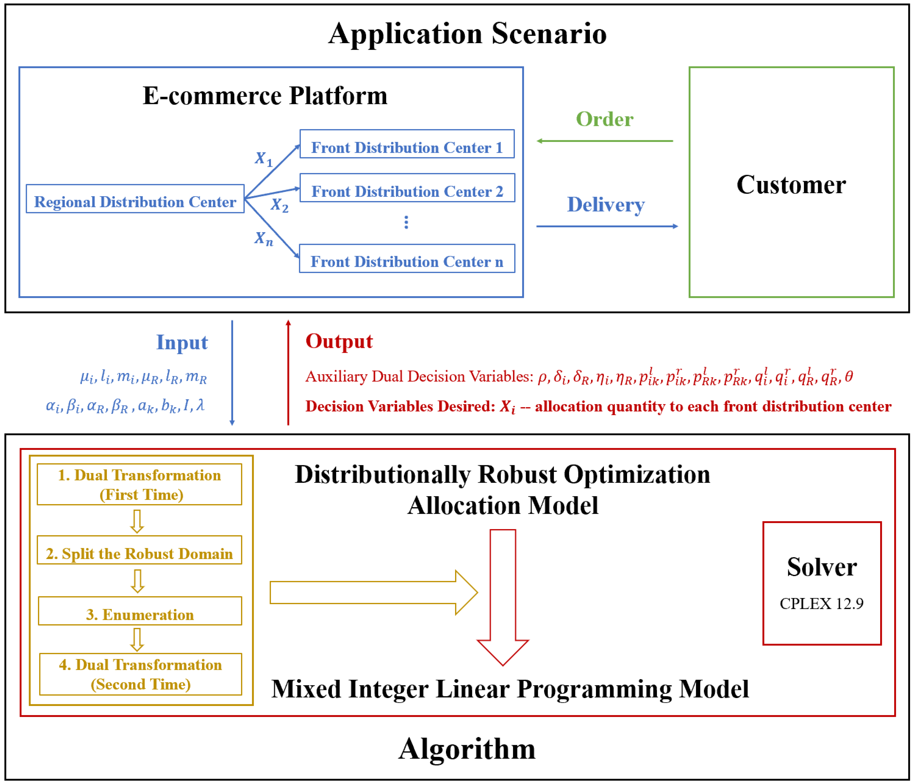
This study focuses on an E-commerce platform distribution network that is structured into distinct regions, with each region containing one regional distribution center and several front distribution centers. As outlined earlier, customer orders are primarily fulfilled by the designated front distribution centers to ensure rapid delivery. However, if the front distribution center runs out of stock, the upstream regional distribution center takes over fulfillment, leading to longer delivery times. If neither the front distribution center nor the regional distribution center can fulfill the order, a lost sale occurs. Additionally, trans-shipments between front distribution centers and reverse logistics from front distribution centers back to the regional distribution center are prohibited. Outside the areas served by front distribution centers, the regional distribution center also handles orders directly for the uncovered portions of the region. The key challenge lies in maximizing front distribution center fulfillment rates to support sales-driven objectives while maintaining a high overall fulfillment rate across the region.

2.1. Basic Model

In order to address the challenge mentioned above, we first establish the deterministic basic model by clarifying the notation and parameter settings, the decision variable, the objective function, and the constraints.

2.1.1. Notation and Parameter Settings

Now, we begin by introducing the notation and parameter settings in this paper.

A.

Notation

Four fundamental notations are as follows:

• Set of merchandises: $\mathcal{W}=1,\dots ,w$, where $w\in \mathcal{W}$ represents the wth merchandise;
• Set of regions: $\mathcal{J}=1,\dots ,J$, where $j\in \mathcal{J}$ represents the jth region;
• Set of front distribution centers: $\mathcal{N}=1,\dots ,N$, where $i\in \mathcal{N}$ represents the ith front distribution center;
• R represents the regional distribution center.

B.

Parameter Settings

Under these notations, we set two parameters as follows:

• Demand vector of merchandise w in region j: ${\mathit{d}}_j^w=(d_{1j}^w,\dots ,d_{Nj}^w,d_{Rj}^w)$, where $d_{ij}^w$ represents the demand of merchandise w in the zone covered by the ith front distribution center in region j and $d_{Rj}^w$ represents the demand of merchandise w in the zone directly served by the regional distribution center in region j;
• Total initial inventory available of merchandise w in region j: $I_j^w$, which is the sum of inventory of merchandise w held at the regional distribution center and the front distribution centers in region j.

Without any loss of generality, we can assume the initial inventory levels in front distribution centers as 0, so that the total initial inventory $I_j^w$ is just equal to the initial inventory of merchandise w held at the regional distribution center in region j.

2.1.2. Decision Variable

Next, we clarify the decision variable of our problem:

• Allocation quantity vector of merchandise w in region j: ${\mathit{X}}_j^w=(X_{1j}^w,\dots ,X_{Nj}^w$), where $X_{ij}^w$ represents the amount of merchandise w allocated to the ith front distribution center in region j.

Actually, we want to decide the inventory levels of merchandise w in the front distribution centers after allocation. However, due to the assumption that the initial inventory levels in the front distribution centers are all 0, the inventory levels of merchandise w in the front distribution centers after allocation are equivalent to the allocation quantities.

2.1.3. Objective Function

We can formulate the basic model as a maximization problem, so our focus now shifts to constructing the objective function. The objective function that we aim to maximize can be established as the following order fulfillment function to meet our requirements:

• Order fulfillment function: ${\sum }_{j\in \mathcal{J}}{\sum }_{w\in \mathcal{W}}{\mathsf{\Gamma }}_j^w({\mathit{X}}_j^w;{\mathit{d}}_j^w,I_j^w)$, where the decision variable is ${\mathit{X}}_j^w$ and the parameters are ${\mathit{d}}_j^w$ and $I_j^w$.

That is to say, the model is

$$\underset{{\mathit{X}}_j^w}{max}\sum _{j\in \mathcal{J}}\sum _{w\in \mathcal{W}}{\mathsf{\Gamma }}_j^w({\mathit{X}}_j^w;{\mathit{d}}_j^w,I_j^w)$$

(1)

This order fulfillment function comprehensively reflects the status of order fulfillment of all merchandises in all regions, and the specific components of the order fulfillment function will be elaborated in detail in the next several parts.

A.

Order Fulfillment Calculation

For a given merchandise w in a specific region j, we can calculate the following types of order fulfillment quantities:

• Orders fulfilled by front distribution center i: ${\mathsf{\Gamma }}_{ij}^w=min(d_{ij}^w,X_{ij}^w)$;
• Orders fulfilled by all front distribution centers: ${\mathsf{\Gamma }}_{Fj}^w={\sum }_{i\in \mathcal{N}}{\mathsf{\Gamma }}_{ij}^w={\sum }_{i\in \mathcal{N}}min(d_{ij}^w,X_{ij}^w)$;
• Orders fulfilled by the regional distribution center:
  ${\mathsf{\Gamma }}_{Rj}^w=min(I_j^w-{\sum }_{i\in \mathcal{N}}{X}_{ij}^w,{\sum }_{i\in \mathcal{N}}max(d_{ij}^w-X_{ij}^w,0)+d_{Rj}^w)$, where the first part $I_j^w-{\sum }_{i\in \mathcal{N}}{X}_{ij}^w$ represents the inventory left in the regional distribution center after allocation and the second part ${\sum }_{i\in \mathcal{N}}max(d_{ij}^w-X_{ij}^w,0)+d_{Rj}^w$ represents the orders needed to be fulfilled by the regional distribution center;
• Orders fulfilled altogether: ${\mathsf{\Gamma }}_{Aj}^w={\mathsf{\Gamma }}_{Fj}^w+{\mathsf{\Gamma }}_{Rj}^w={\sum }_{i\in \mathcal{N}}{\mathsf{\Gamma }}_{ij}^w+{\mathsf{\Gamma }}_{Rj}^w$
  $={\sum }_{i\in \mathcal{N}}min(d_{ij}^w,X_{ij}^w)+min(I_j^w-{\sum }_{i\in \mathcal{N}}{X}_{ij}^w,{\sum }_{i\in \mathcal{N}}max(d_{ij}^w-X_{ij}^w,0)+d_{Rj}^w)$.

B.

Lost Sales Calculation

However, excessively allocating inventories to downstream front distribution centers may cause inventory shortage in the regional distribution center, which will eventually incur lost sales in the region. For a given merchandise w in a specific region j, the lost sales can be calculated as follows:

• Orders could be fulfilled if there is no allocation: ${\mathsf{\Gamma }}_{Cj}^w=min(I_j^w,{\sum }_{i\in \mathcal{N}}{d}_{ij}^w+d_{Rj}^w)$;
• Orders actually fulfilled: ${\mathsf{\Gamma }}_{Aj}^w={\mathsf{\Gamma }}_{Fj}^w+{\mathsf{\Gamma }}_{Rj}^w={\sum }_{i\in \mathcal{N}}{\mathsf{\Gamma }}_{ij}^w+{\mathsf{\Gamma }}_{Rj}^w$, which has been derived in the previous part;
• Lost sales caused by allocation: ${\Delta }_j^w={\mathsf{\Gamma }}_{Cj}^w-{\mathsf{\Gamma }}_{Aj}^w={\mathsf{\Gamma }}_{Cj}^w-{\mathsf{\Gamma }}_{Fj}^w-{\mathsf{\Gamma }}_{Rj}^w={\mathsf{\Gamma }}_{Cj}^w-{\sum }_{i\in \mathcal{N}}{\mathsf{\Gamma }}_{ij}^w-{\mathsf{\Gamma }}_{Rj}^w$, which is the gap between the quantity of orders could be fulfilled if there is no allocation and the quantity of orders actually fulfilled.

C.

Balance Coefficient Setting

After we have calculated the quantity of orders fulfilled by front distribution centers and the lost sales caused by allocation, we now introduce a balance coefficient to align with the goal of improving front distribution centers’ fulfillment rates while also maintaining the region’s overall fulfillment rate:

• Balance coefficient: $\lambda$, which can be adjusted according to the specific requirements of the platform.

The choice of $\lambda$ depends on whether the platform prefers to increase the front distribution center fulfillment rate as much as possible or needs to control the loss caused by excessive allocation within a certain extent.

Eventually, through the above calculations of order fulfillment and lost sales and the setting of balance coefficient, our objective function can be derived as follows:

$$\begin{array}{cc}\hfill \sum _{j\in \mathcal{J}}\sum _{w\in \mathcal{W}}{\mathsf{\Gamma }}_j^w({\mathit{X}}_j^w;{\mathit{d}}_j^w,I_j^w)& =\sum _{j\in \mathcal{J}}\sum _{w\in \mathcal{W}}({\mathsf{\Gamma }}_{Fj}^w-\lambda ·{\Delta }_j^w)\hfill \end{array}$$

(2)

$$\begin{array}{cc}\hfill & =\sum _{j\in \mathcal{J}}\sum _{w\in \mathcal{W}}\sum _{i\in \mathcal{N}}{\mathsf{\Gamma }}_{ij}^w-\lambda \sum _{j\in \mathcal{J}}\sum _{w\in \mathcal{W}}({\mathsf{\Gamma }}_{Cj}^w-\sum _{i\in \mathcal{N}}{\mathsf{\Gamma }}_{ij}^w-{\mathsf{\Gamma }}_{Rj}^w)\hfill \end{array}$$

(3)

$$\begin{array}{cc}\hfill & =(1+\lambda )\sum _{j\in \mathcal{J}}\sum _{w\in \mathcal{W}}\sum _{i\in \mathcal{N}}{\mathsf{\Gamma }}_{ij}^w-\lambda \sum _{j\in \mathcal{J}}\sum _{w\in \mathcal{W}}({\mathsf{\Gamma }}_{Cj}^w-{\mathsf{\Gamma }}_{Rj}^w)\hfill \end{array}$$

(4)

where ${\mathsf{\Gamma }}_{ij}^w=min(d_{ij}^w,X_{ij}^w)$, ${\mathsf{\Gamma }}_{Rj}^w=min(I_j^w-{\sum }_{i\in \mathcal{N}}{X}_{ij}^w,{\sum }_{i\in \mathcal{N}}max(d_{ij}^w-X_{ij}^w,0)+d_{Rj}^w)$ and ${\mathsf{\Gamma }}_{Cj}^w=min(I_j^w,{\sum }_{i\in \mathcal{N}}{d}_{ij}^w+d_{Rj}^w)$.

2.1.4. Constraints

In our basic model, there are two constraints:

• Total inventory constraint: ${\sum }_{i\in \mathcal{N}}{X}_{ij}^w\le I_j^w,\forall j\in \mathcal{J},w\in \mathcal{W}$;
• Integer constraint: $X_{ij}^w\in {\mathbb{Z}}_{+},{\rho }_{ij}^w\in \{0,1\},\forall i\in \mathcal{N},j\in \mathcal{J},w\in \mathcal{W}$.

2.2. Distributionally Robust Optimization

It is not difficult to find that determining the optimal allocation in the above basic model necessitates some knowledge of demand distributions, while accurately predicting the true demand distributions usually faces huge challenges. Therefore, we apply the method of distributionally robust optimization to tackle such difficulty.

2.2.1. Objective Function

In the case of distributionally robust optimization, due to the uncertainty of demand, the objective function should be modified to the following form:

$$\underset{({\mathbb{P}}_j^w,j\in \mathcal{J},w\in \mathcal{W})\in \mathcal{G}}{min}{\mathbb{E}}_{{\mathbb{P}}_j^w}\left[\sum _{j\in \mathcal{J}}\sum _{w\in \mathcal{W}}{\mathsf{\Gamma }}_j^w({\mathit{X}}_j^w;{\mathit{d}}_j^w,I_j^w)\right]$$

(5)

where $\mathcal{G}$ is the ambiguity set, ${\mathbb{P}}_j^w$ is the probability measure on the probability space of random variables $d_{ij}^w,i\in \mathcal{N}$, and $d_{Rj}^w$ is in demand vector ${\mathit{d}}_j^w$.

That is to say, the modified distributionally robust optimization model is

$$\underset{{\mathit{X}}_j^w}{max}\underset{({\mathbb{P}}_j^w,j\in \mathcal{J},w\in \mathcal{W})\in \mathcal{G}}{min}{\mathbb{E}}_{{\mathbb{P}}_j^w}\left[\sum _{j\in \mathcal{J}}\sum _{w\in \mathcal{W}}{\mathsf{\Gamma }}_j^w({\mathit{X}}_j^w;{\mathit{d}}_j^w,I_j^w)\right]$$

(6)

2.2.2. Ambiguity Set

Naturally, according to the modified objective function shown above, the next step is to construct an appropriate ambiguity set $\mathcal{G}$ for random variables $d_{ij}^w,i\in \mathcal{N}$, and $d_{Rj}^w$ in demand vector ${\mathit{d}}_j^w$. The ambiguity set $\mathcal{G}$ can be constructed as follows:

$$\mathcal{G}=\left\{{\mathbb{P}}_j^w\in \mathcal{P}\left|\begin{array}{c}{\mathit{d}}_j^w\sim {\mathbb{P}}_j^w\\ d_{ij}^w\in W_{d_{ij}^w}=[l_{ij}^w,m_{ij}^w],d_{Rj}^w\in W_{d_{Rj}^w}=[l_{Rj}^w,m_{Rj}^w]\\ {\mathbb{E}}_{{\mathbb{P}}_j^w}\left[d_{ij}^w\right]={\mu }_{ij}^w,{\mathbb{E}}_{{\mathbb{P}}_j^w}\left[d_{Rj}^w\right]={\mu }_{Rj}^w\\ {\mathbb{E}}_{{\mathbb{P}}_j^w}[\underset{k}{max}(a_k|d_{ij}^w-{\mu }_{ij}^w|+b_k)]\le {({\alpha }_{ij}^w{\mu }_i+{\beta }_{ij}^w)}^2\\ {\mathbb{E}}_{{\mathbb{P}}_j^w}[\underset{k}{max}(a_k|d_{Rj}^w-{\mu }_{Rj}^w|+b_k)]\le {({\alpha }_{Rj}^w{\mu }_{Rj}^w+{\beta }_{Rj}^w)}^2\\ k\in \{1,\dots ,K\},i\in \mathcal{N},j\in \mathcal{J},w\in \mathcal{W}\end{array}\right.\right\}$$

where $\mathcal{P}$ is the set of probability measures ${\mathbb{P}}_j^w$; ${\mu }_{ij}^w$, $l_{ij}^w$, and $m_{ij}^w$ are the forecasted mean, lower bound, and upper bound of the demand of merchandise w in the ith-front-distribution-center-covered region in region j; ${\mu }_{Rj}^w$, $l_{Rj}^w$, and $m_{Rj}^w$ are the forecasted mean, lower bound, and upper bound of the demand of merchandise w in the regional-distribution-center-directly-covered region in region j; and ${\alpha }_{ij}^w$, ${\beta }_{ij}^w$, ${\alpha }_{Rj}^w$, ${\beta }_{Rj}^w$,$a_k$, and $b_k$ are given parameters.

The forecasted mean, lower bound, and upper bound of demand are obtained from historical sales data mainly using the AutoRegressive Integrated Moving-Average Model. (AutoRegressive Integrated Moving-Average Model is a widely used statistical model for time-series analysis and forecasting. The fundamental idea behind it is to model the time series as a combination of its past values and past forecast errors, in order to capture patterns and trends in the historical data [36]). Additionally, through the analysis of historical sales data, we discover that there is a certain correlation between the mean and variance of the sales volume, so we introduce the parameters ${\alpha }_{ij}^w$, ${\beta }_{ij}^w$, ${\alpha }_{Rj}^w$, and ${\beta }_{Rj}^w$ to reflect this correlation, and these parameters are also determined by the historical sales data. Since we want to reveal the impact of moment information in demand forecasting on the distributionally robust fulfillment rate improvement algorithm, this helps us to discover how demand forecasting influences the allocation rule and how forecasted variance influences the fulfillment rates at fixed or changing inventory levels.

Another point is that we use $\mathbb{E}[{max}_k(a_k|d-\mu |+b_k)]\le {(\alpha \mu +\beta )}^2,k\in \{1,\dots ,K\}$, as an approximation of $\mathbb{E}\left[{(d-\mu )}^2\right]\le {(\alpha \mu +\beta )}^2$ to describe the volatility of the mean value of the forecast demand. From a theoretical perspective, this signifies that we use ${max}_k(a_k|x|+b_k),k\in \{1,\dots ,K\}$, the maximum of a series of linear functions, to approximate ${|x|}^2$, the quadratic function, where $a_k$ and $b_k$ represent the slope and intercept of the kth approximating linear function.

2.2.3. Distributionally Robust Optimization Model

Now, we can combine the modified objective function, the moment-based ambiguity set, and all the other constraints to formulate the complete distributionally robust optimization model as follows:

$$\underset{{\mathit{X}}_j^w}{max}\underset{({\mathbb{P}}_j^w,j\in \mathcal{J},w\in \mathcal{W})\in \mathcal{G}}{min}{\mathbb{E}}_{{\mathbb{P}}_j^w}\left[\sum _{j\in \mathcal{J}}\sum _{w\in \mathcal{W}}{\mathsf{\Gamma }}_j^w({\mathit{X}}_j^w;{\mathit{d}}_j^w,I_j^w)\right]$$

(7)

s.t.

$$\mathcal{G}=\left\{{\mathbb{P}}_j^w\in \mathcal{P}\left|\begin{array}{c}{\mathit{d}}_j^w\sim {\mathbb{P}}_j^w\\ d_{ij}^w\in W_{d_{ij}^w}=[l_{ij}^w,m_{ij}^w],d_{Rj}^w\in W_{d_{Rj}^w}=[l_{Rj}^w,m_{Rj}^w]\\ {\mathbb{E}}_{{\mathbb{P}}_j^w}\left[d_{ij}^w\right]={\mu }_{ij}^w,{\mathbb{E}}_{{\mathbb{P}}_j^w}\left[d_{Rj}^w\right]={\mu }_{Rj}^w\\ {\mathbb{E}}_{{\mathbb{P}}_j^w}[\underset{k}{max}(a_k|d_{ij}^w-{\mu }_{ij}^w|+b_k)]\le {({\alpha }_{ij}^w{\mu }_i+{\beta }_{ij}^w)}^2\\ {\mathbb{E}}_{{\mathbb{P}}_j^w}[\underset{k}{max}(a_k|d_{Rj}^w-{\mu }_{Rj}^w|+b_k)]\le {({\alpha }_{Rj}^w{\mu }_{Rj}^w+{\beta }_{Rj}^w)}^2\\ k\in \{1,\dots ,K\},i\in \mathcal{N},j\in \mathcal{J},w\in \mathcal{W}\end{array}\right.\right\}$$

$$\begin{array}{cc}\hfill \sum _{j\in \mathcal{J}}\sum _{w\in \mathcal{W}}{\mathsf{\Gamma }}_j^w({\mathit{X}}_j^w;{\mathit{d}}_j^w,I_j^w)& =(1+\lambda )\sum _{j\in \mathcal{J}}\sum _{w\in \mathcal{W}}\sum _{i\in \mathcal{N}}{\mathsf{\Gamma }}_{ij}^w-\lambda \sum _{j\in \mathcal{J}}\sum _{w\in \mathcal{W}}({\mathsf{\Gamma }}_{Cj}^w-{\mathsf{\Gamma }}_{Rj}^w)\hfill \end{array}$$

(8)

$$\begin{array}{cc}\hfill {\mathsf{\Gamma }}_{ij}^w& =min(d_{ij}^w,X_{ij}^w)\hfill \end{array}$$

(9)

$$\begin{array}{cc}\hfill {\mathsf{\Gamma }}_{Rj}^w& =min(I_j^w-\sum _{i\in \mathcal{N}}{X}_{ij}^w,\sum _{i\in \mathcal{N}}max(d_{ij}^w-X_{ij}^w,0)+d_{Rj}^w)\hfill \end{array}$$

(10)

$$\begin{array}{cc}\hfill {\mathsf{\Gamma }}_{Cj}^w& =min(I_j^w,\sum _{i\in \mathcal{N}}{d}_{ij}^w+d_{Rj}^w)\hfill \end{array}$$

(11)

$$\begin{array}{cc}\hfill \sum _{i\in \mathcal{N}}{X}_{ij}^w& \le I_j^w,\forall j\in \mathcal{J},w\in \mathcal{W}\hfill \end{array}$$

(12)

$$\begin{array}{cc}\hfill X_{ij}^w\in {\mathbb{Z}}_{+},{\rho }_{ij}^w& \in \{0,1\},\forall i\in \mathcal{N},j\in \mathcal{J},w\in \mathcal{W}\hfill \end{array}$$

(13)

2.3. Transformation and Approximation

After establishing the distributionally robust optimization model by clarifying the modified objective function with the moment-based ambiguity set, we now focus on how to transform the model into a solvable algorithm.

Upon examining the model, we can find that the basic module in our problem is a 1-N two-echelon distribution network with a single product, i.e., one regional distribution center allocating inventories of one product to N front distribution centers. Therefore, the following transformation and approximation of the distributionally robust optimization model are based on this basic module (in short, we can set j and w aside for now and keep only i and R as notations in the subsequent derivations). We first express Problem (5) together with the constraint of the ambiguity set in an integral form, and subsequently perform a dual transformation. In detail, set the dual variables of constraints (1) $\int dF=1$, (2) $\int {max}_k(a_k|d_i-{\mu }_i|+b_k)dF\le {({\alpha }_i{\mu }_i+{\beta }_i)}^2,\forall i\in \mathcal{N}$, (3) $\int {max}_k(a_k|d_R-{\mu }_R|+b_k)dF\le {({\alpha }_R{\mu }_R+{\beta }_R)}^2$, (4) $\int d_{i}dF={\mu }_i,\forall i\in \mathcal{N}$ and (5) $\int d_{R}dF={\mu }_R$ as $\rho$, ${\delta }_i$, ${\delta }_R$, ${\eta }_i$, and ${\eta }_R$, respectively. Then, we have Theorem 1.

Theorem 1. 

The dual problem under a given allocation $\mathit{X}$ is

$$\begin{array}{c} \hspace{1em}\hspace{1em}\underset{\rho ,{\delta }_i,{\delta }_R,{\eta }_i,{\eta }_R}{max}\rho +\sum _{i\in \mathcal{N}}{\mu }_i{\eta }_i+{\mu }_R{\eta }_R+\sum _{i\in \mathcal{N}}{({\alpha }_i{\mu }_i+{\beta }_i)}^2{\delta }_i+{({\alpha }_R{\mu }_R+{\beta }_R)}^2{\delta }_R\hfill \\ s.t.\hspace{1em}\rho +\sum _i{d}_i{\eta }_i+d_R{\eta }_R+\sum _i\underset{k}{max}(a_k|d_i-{\mu }_i|+b_k){\delta }_i+\underset{k}{max}(a_k|d_R-{\mu }_R|+b_k){\delta }_R\hfill \\ \hspace{1em}\hspace{1em}\hspace{1em}\le \mathsf{\Gamma }(\mathit{X},\mathit{d},I)=(1+\lambda )\sum _{i\in \mathcal{N}}{\mathsf{\Gamma }}_i-\lambda ({\mathsf{\Gamma }}_C-{\mathsf{\Gamma }}_R)=(1+\lambda )\sum _{i\in \mathcal{N}}{\mathsf{\Gamma }}_i+\lambda {\mathsf{\Gamma }}_R-\lambda {\mathsf{\Gamma }}_C,\hfill \end{array}$$

(14)

$$\begin{array}{c}\forall \mathit{d}\in [\mathit{l},\mathit{m}]=[l_1,m_1]\times \dots \times [l_N,m_N]\times [l_R,m_R]\hfill \end{array}$$

(15)

$$\begin{array}{c}\rho \in \mathbb{R},{\delta }_R\le 0,{\eta }_R\in \mathbb{R},{\delta }_i\le 0,{\eta }_i\in \mathbb{R},\forall i\in \mathcal{N}.\hfill \end{array}$$

(16)

Naturally, now we focus on transforming Inequality (15) into a solvable problem. In the previous literature such as [37], they broadly deal with a sum of a series of minimum terms on one side of the inequality. However, due to the existence of the term $-\lambda {\mathsf{\Gamma }}_C$, which is a minus minimum term since ${\mathsf{\Gamma }}_C=min(I,{\sum }_{i\in \mathcal{N}}{d}_i+d_R)$, their method is no longer applicable. To tackle this issue, we follow the method developed by [16], which divides the domain of demand vector $\mathit{d}$ into several sub-domains and constructs equivalent constraints for each sub-domain. In detail, we divide the domain $\mathcal{A}=[\mathit{l},\mathit{m}]$ into two sub-domains ${\mathcal{A}}_1=\{\mathit{d}|{\sum }_{i\in \mathcal{N}}{d}_i+d_R\ge I\}\cap \mathcal{A}$ and ${\mathcal{A}}_2=\{\mathit{d}|{\sum }_{i\in \mathcal{N}}{d}_i+d_R\le I\}\cap \mathcal{A}$ such that $\mathcal{A}={\mathcal{A}}_1\cup {\mathcal{A}}_2$. Then, we present the derivation process of one sub-constraint as an example, noting that the derivation methods for the remaining sub-constraints are analogous. As in [16], we define such a symbol vector ${\mathit{Y}}^{\mathit{e}}=(Y_1^{\mathit{e}},\dots ,Y_N^{\mathit{e}})$, where $\mathit{e}\in {\left\{0,1\right\}}^N$ such that $Y_i^{\mathit{e}}$ represents $d_i$ if $e_i=1$ and represents $X_i$ if $e_i=0$. To elaborate further, ${\sum }_{i\in \mathcal{N}}{\mathsf{\Gamma }}_i={\sum }_{i\in \mathcal{N}}min(d_i,X_i)={min}_{\mathit{e}\in {\{0,1\}}^N}\left\{{\sum }_{i\in \mathcal{N}}{Y}_i^{\mathit{e}}\right\}$. Hence, with the condition $I+{\sum }_{i\in \mathcal{N}}{\mathsf{\Gamma }}_i\le {\sum }_{i\in \mathcal{N}}{d}_i+d_R+{\sum }_{i\in \mathcal{N}}{X}_i$ and ${\sum }_{i\in \mathcal{N}}{d}_i+d_R\ge I$, one sub-constraint is

$$\begin{array}{cc}\hfill \rho +\sum _i{d}_i{\eta }_i+d_R{\eta }_R+\sum _i\underset{k}{max}& (a_k|d_i-{\mu }_i|+b_k){\delta }_i+\underset{k}{max}(a_k|d_R-{\mu }_R|+b_k){\delta }_R\hfill \end{array}$$

$$\begin{array}{cc}\hfill & \le (\lambda +1)\sum _{i\in \mathcal{N}}{\mathsf{\Gamma }}_i-\lambda \sum _{i\in \mathcal{N}}{X}_i,\forall \mathit{d}\in {\mathcal{A}}_1\hfill \end{array}$$

(17)

$$\begin{array}{cc}\hfill & =(\lambda +1)\sum _{i\in \mathcal{N}}{Y}_i^{\mathit{e}}-\lambda \sum _{i\in \mathcal{N}}{X}_i,\forall \mathit{d}\in {\mathcal{A}}_1,\mathit{e}\in {\{0,1\}}^N.\hfill \end{array}$$

(18)

According to our research on the distribution network structures of major E-commerce platforms, the number of front distribution centers in each region is not large in reality (usually 1 to 3), so we can enumerate $\mathit{e}\in {\{0,1\}}^N$ and reformulate the constraints for each $\mathit{e}$. For instance, when $N=3$ and $\mathit{e}=(1,0,0)$, one enumeration of Sub-Constraint (18) as follows:

$$\begin{array}{cc}\hfill \rho & +d_1{\eta }_1+d_2{\eta }_2+d_3{\eta }_3+d_R{\eta }_R+\underset{k}{max}(a_k|d_1-{\mu }_1|+b_k){\delta }_1\hfill \\ \hfill & +\underset{k}{max}(a_k|d_2-{\mu }_2|+b_k){\delta }_2+\underset{k}{max}(a_k|d_3-{\mu }_3|+b_k){\delta }_3+\underset{k}{max}(a_k|d_R-{\mu }_R|+b_k){\delta }_R\hfill \\ \hfill & \le (\lambda +1)(d_1+X_2+X_3)-\lambda (X_1+X_2+X_3)=(\lambda +1)d_1-\lambda X_1+X_2+X_3,\forall \mathit{d}\in {\mathcal{A}}_1.\hfill \end{array}$$

(19)

Since the demand parameters $d_1,d_2,d_3,d_R$ and the allocaiton quantities $X_1,X_2,X_3$ as decision variables are both integers while all the other parameters and decision variables are continuous, naturally, the enumeration case in (19) can be viewed as a mixed-integer problem. Then, we place the variables with remaining constraints on the left side of the inequality as $z_l=d_1{\eta }_1+d_2{\eta }_2+d_3{\eta }_3+d_R{\eta }_R+{max}_k(a_k|d_1-{\mu }_1|+b_k){\delta }_1+{max}_k(a_k|d_2-{\mu }_2|+b_k){\delta }_2+{max}_k(a_k|d_3-{\mu }_3|+b_k){\delta }_3+{max}_k(a_k|d_R-{\mu }_R|+b_k){\delta }_R$ and the rest on the right side as $z_r=\rho -\lambda X_1+X_2+X_3$. To always ensure the condition that $z_l\le z_r$, we need to maximize $z_l$ by maximizing $d_1({\eta }_1-\lambda -1)+d_2{\eta }_2+d_3{\eta }_3+d_R{\eta }_R+v_1{\delta }_1+v_2{\delta }_2+v_3{\delta }_3+v_R{\delta }_R$, where $v_i\ge {max}_k(a_k|d_i-{\mu }_i|+b_k)$, $v_R\ge {max}_k(a_k|d_R-{\mu }_R|+b_k)$, $l_i\le d_i\le m_i$, $l_R\le d_R\le m_R$ and ${\sum }_{i\in \mathcal{N}}{d}_i+d_R\ge I$. Then, an equivalent dual problem can be achieved as follows.

Theorem 2. 

The equivalent dual problem is

$$\begin{array}{cc}\hfill & min{z}_d=\sum _i\left[m_i{q}_i^l-l_i{q}_i^r+\sum _k\left[(a_k{\mu }_i-b_k)p_{ik}^l-(a_k{\mu }_i+b_k)p_{ik}^r\right]\right]\hfill \end{array}$$

$$\begin{array}{cc}\hfill & +m_R{q}_R^l-l_R{q}_R^r+\sum _k\left[(a_k{\mu }_R-b_k)p_{Rk}^l-(a_k{\mu }_R+b_k)p_{Rk}^r\right]-I·\theta \hfill \end{array}$$

(20)

$$\begin{array}{cc}\hfill s.t.& q_1^l-q_1^r+\sum _k(a_k{p}_{1k}^l-a_k{p}_{1k}^r)-\theta ={\eta }_1-\lambda -1\hfill \end{array}$$

(21)

$$\begin{array}{cc}\hfill & q_2^l-q_2^r+\sum _k(a_k{p}_{2k}^l-a_k{p}_{2k}^r)-\theta ={\eta }_2\hfill \end{array}$$

(22)

$$\begin{array}{cc}\hfill & q_3^l-q_3^r+\sum _k(a_k{p}_{3k}^l-a_k{p}_{3k}^r)-\theta ={\eta }_3\hfill \end{array}$$

(23)

$$\begin{array}{cc}\hfill & q_R^l-q_R^r+\sum _k(a_k{p}_{Rk}^l-a_k{p}_{Rk}^r)-\theta ={\eta }_R\hfill \end{array}$$

(24)

$$\begin{array}{cc}\hfill & \sum _k(-p_{Rk}^l-p_{Rk}^r)={\delta }_R\hfill \end{array}$$

(25)

$$\begin{array}{cc}\hfill & \sum _k(-p_{ik}^l-p_{ik}^r)={\delta }_i,\forall i\in \left\{1,2,3\right\}\hfill \end{array}$$

(26)

$$\begin{array}{cc}\hfill & q_R^l\ge 0,q_R^r\ge 0,\theta \ge 0,q_i^l\ge 0,q_i^r\ge 0,\forall i\in \left\{1,2,3\right\}\hfill \end{array}$$

(27)

$$\begin{array}{cc}\hfill & p_{Rk}^l\ge 0,p_{Rk}^r\ge 0,p_{ik}^l\ge 0,p_{ik}^r\ge 0,\forall k\in \{1,\dots ,K\},i\in \left\{1,2,3\right\}\hfill \end{array}$$

(28)

Proof. 

The original maximization problem is

$$\begin{array}{cc}\hfill & max{z}_l=d_1({\eta }_1-\lambda -1)+d_2{\eta }_2+d_3{\eta }_3+d_R{\eta }_R+v_1{\delta }_1+v_2{\delta }_2+v_3{\delta }_3+v_R{\delta }_R\hfill \end{array}$$

$$\begin{array}{cc}\hfill \mathrm{s}.\mathrm{t}.& v_i\ge a_k(d_i-{\mu }_i)+b_k,\forall i\in \left\{1,2,3\right\},k\in \{1,\dots ,K\}\hfill \end{array}$$

(29)

$$\begin{array}{cc}\hfill & v_i\ge -a_k(d_i-{\mu }_i)+b_k,\forall i\in \left\{1,2,3\right\},k\in \{1,\dots ,K\}\hfill \end{array}$$

(30)

$$\begin{array}{cc}\hfill & v_R\ge a_k(d_R-{\mu }_R)+b_k,k\in \{1,\dots ,K\}\hfill \end{array}$$

(31)

$$\begin{array}{cc}\hfill & v_R\ge -a_k(d_R-{\mu }_R)+b_k,k\in \{1,\dots ,K\}\hfill \end{array}$$

(32)

$$\begin{array}{cc}\hfill & l_i\le d_i,\forall i\in \left\{1,2,3\right\}\hfill \end{array}$$

(33)

$$\begin{array}{cc}\hfill & d_i\le m_i,\forall i\in \left\{1,2,3\right\}\hfill \end{array}$$

(34)

$$\begin{array}{cc}\hfill & l_R\le d_R\hfill \end{array}$$

(35)

$$\begin{array}{cc}\hfill & d_R\le m_R\hfill \end{array}$$

(36)

$$\begin{array}{cc}\hfill & \sum _{i\in \mathcal{N}}{d}_i+d_R\ge I\hfill \end{array}$$

(37)

Now, we perform the dual transformation by setting the following series of dual variables corresponding to the constraints in the original maximization problem:

• Set $p_{ik}^l$ as the dual variables of the constraints $v_i\ge a_k(d_i-{\mu }_i)+b_k,\forall i\in \left\{1,2,3\right\},k\in \{1,\dots ,K\}$;
• Set $p_{ik}^r$ as the dual variables of the constraints $v_i\ge -a_k(d_i-{\mu }_i)+b_k,\forall i\in \left\{1,2,3\right\},k\in \{1,\dots ,K\}$;
• Set $p_{Rk}^l$ as the dual variables of the constraints $v_R\ge a_k(d_R-{\mu }_R)+b_k,k\in \{1,\dots ,K\}$;
• Set $p_{Rk}^r$ as the dual variables of the constraints $v_R\ge -a_k(d_R-{\mu }_R)+b_k,k\in \{1,\dots ,K\}$;
• Set $q_i^l$ as the dual variables of the constraints $l_i\le d_i,\forall i\in \left\{1,2,3\right\}$;
• Set $q_i^r$ as the dual variables of the constraints $d_i\le m_i,\forall i\in \left\{1,2,3\right\}$;
• Set $q_R^l$ as the dual variable of the constraint $l_R\le d_R$;
• Set $q_R^r$ as the dual variable of the constraint $d_R\le m_R$;
• Set $\theta$ as the dual variable of the constraint ${\sum }_{i\in \mathcal{N}}{d}_i+d_R\ge I$.

Then, we can obtain the equivalent dual minimization problem with dual constraints of the dual variables as shown in Theorem 2. □

In Theorem 2, $p_{ik}^l,p_{ik}^r,p_{Rk}^l,p_{Rk}^r,q_i^l,q_i^r,q_R^l,q_R^r,\theta ,{\eta }_i,{\eta }_R,{\delta }_i,{\delta }_R$ are all decision variables, while $m_i,l_i,{\mu }_i,m_R,l_R,{\mu }_R,a_k,b_k,I,\lambda$ are given parameters. Then, we can find that the objective function and Constraints (21)–(28) are all linear combinations of the decision variables and given parameters. So, together with the constraint $z_d\le z_r$ and Constraints (21)–(28), we can obtain a mixed-integer linear programming model for the sub-constraint (18). Accordingly, we can also construct a robust counterpart for every constraint generated from the original distributionally robust optimization model, similar to Sub-Constraint (18), and eventually obtain a complete mixed-integer linear programming model. In Appendix A, we provide a complete mixed-integer linear programming model for the case with $N=3$.

2.4. Algorithm

Now, we introduce the details of the distributionally robust allocation algorithm as the flow chart shown in Figure 1.

Detailedly, we should input the forecasted mean, lower bound, and upper bound of demand in the ith-front-distribution-center-covered region and the directly regional-distribution-center-covered region ${\mu }_i,l_i,m_i,{\mu }_R,l_R,m_R$, the given parameters related to the correlation with the mean and variance ${\alpha }_i,{\beta }_i,{\alpha }_R,{\beta }_R$, the slope and intercept of the kth approximating linear function $a_k,b_k$, the total available inventory I, and the balance coefficient $\lambda$ as the input parameters. Then, we directly solve this mixed-integer linear programming model in Python 3.8 with CPLEX 12.9 as the solver (IBM ILOG CPLEX Optimization Studio, CPLEX in short, is an optimization software package which can efficiently solve mixed-integer programming problems. The principle behind CPLEX for solving mixed-integer linear programming problems is primarily based on the Branch and Bound method, combined with efficient linear programming solvers and various optimization techniques [38]). Finally, we can obtain the optimal solution solved by CPLEX, where ${\eta }_i,{\eta }_R,{\delta }_i,{\delta }_R,p_{ik}^l,p_{ik}^r,p_{Rk}^l,p_{Rk}^r,q_i^l,q_i^r,q_R^l,q_R^r,\theta$ are the auxiliary dual decision variables and $X_i,i\in \mathcal{N}$ are the allocation quantities to each front distribution center that we desire to know.

3. Numerical Experiment

In this section, we comprehensively discover the influences of moment information in demand forecasting on the distributionally robust fulfillment rate improvement algorithm by successively answering the following two vital questions: 1. How does demand forecasting influence the allocation rule? 2. How does forecasted variance influence the fulfillment rates?

3.1. Experiments on Synthetic Data

We first carry out three single-stage allocation experiments altogether to reveal the influences of three parameters, consisting of the forecasted mean, variance, and bounds (including the lower bound and the upper bound) of demand in each front-distribution-center-covered region on the allocation quantity to each front distribution center under different total available inventory conditions, aiming to reflect the corresponding optimal allocation rule under different circumstances. In this group of experiments, we do not have to care about the demand in the directly regional-distribution-center-covered region, so we can just directly set $\lambda =0$. And, in general, the allocation quantity to each front distribution center increases with the total available inventory, naturally.

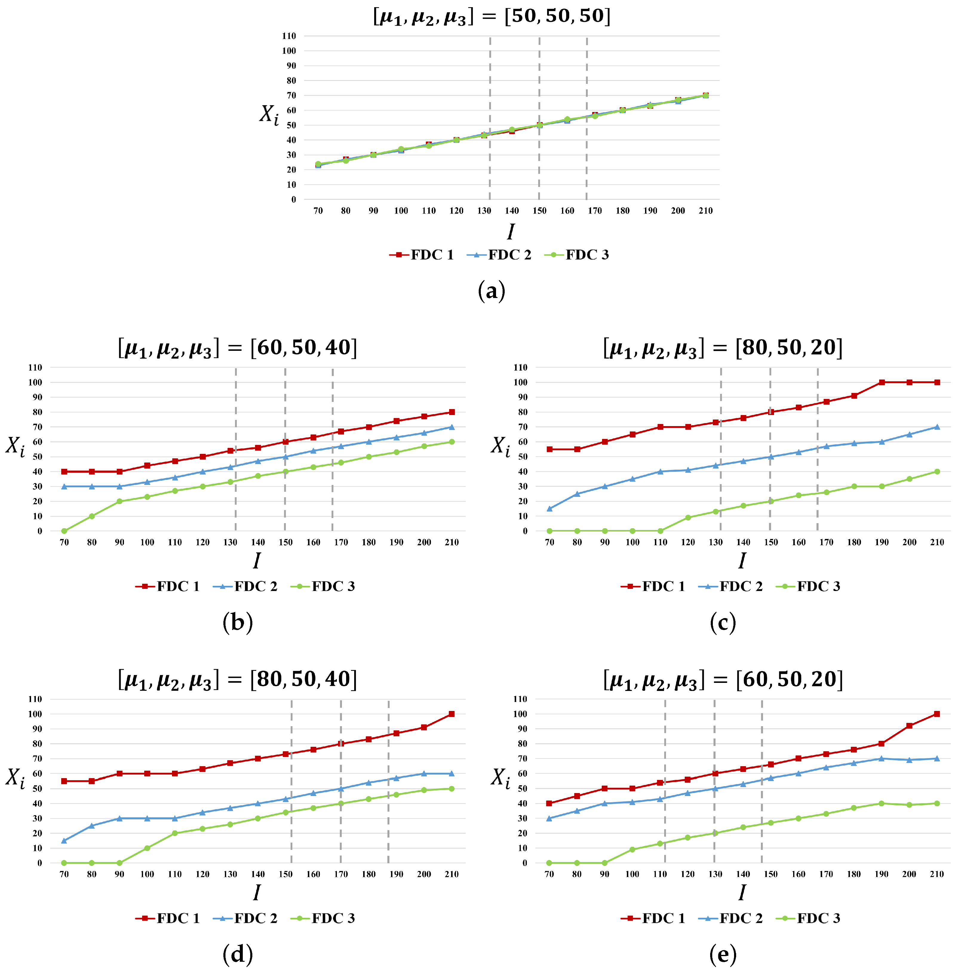
3.1.1. Experiment 1: Impact of Forecasted Mean on the Allocation Rule

In this experiment, we reveal the impact of forecasted mean of demand in each front-distribution-center-covered region on the allocation quantity to each front distribution center under different total available inventory conditions. The parameter setting of this experiment is shown in

Table 2. Parameter setting of Experiment 1.

	${\sigma }_i^2$					$l_i$				$m_i$
FDC 1 †
FDC 2	25					0				100
FDC 3
$\lambda =0$
	${\mu }_i$
FDC 1	50			60		80				80		60
FDC 2	50			50		50				50		50
FDC 3	50			40		20				40		20
I
70	80	90	100	110	120	130	140	150	160	170	180	190	200	210

† FDC: Front Distribution Center.

.

From Figure 2 (the three gray dotted lines in the figure from left to right, respectively, indicate $I=\widehat{\mu }-2\widehat{\sigma }$, $I=\widehat{\mu }$, and $I=\widehat{\mu }+2\widehat{\sigma }$, where $\widehat{\mu }={\sum }_{i=1}^3{\mu }_i$ and $\widehat{\sigma }=\sqrt{{\displaystyle \frac{1}{3}}{\sum }_{i=1}^3{\sigma }_i^2}$), we can find that when the total available inventory is sufficient: the allocation quantity to each front distribution center is almost directly proportional to the forecasted mean of demand in each front-distribution-center-covered region. However, when the total available inventory is insufficient, all the available inventory will first be allocated to the region with larger forecasted demand. Moreover, through observation and calculation, it can be found that, when total available inventory is less than ${\sum }_{i=1}^3{\mu }_i-4\sqrt{{\displaystyle \frac{1}{3}}{\sum }_{i=1}^3{\sigma }_i^2}$, the allocation quantity to the region with the smallest forecasted demand is zero. The reason is that, when the variances of these three regions’ forecasted demand are equal, the one with the smallest mean will have the largest volatility, which means the largest risk of unsalable commodities. Therefore, higher priority will be given to the region with the larger forecasted mean of demand in order to ensure the basic sales volume, as much as possible.

3.1.2. Experiment 2: Impact of Forecasted Variance on the Allocation Rule

In this experiment, we reveal the impact of the variance of the forecasted demand in each front-distribution-center-covered region on the allocation quantity to each front distribution center under different total available inventory conditions. The parameter setting of this experiment is shown in

Table 3. Parameter setting of Experiment 2.

	${\mu }_i$					$l_i$				$m_i$
FDC 1 †
FDC 2	50					0				100
FDC 3
$\lambda =0$
	${\sigma }_i^2$
FDC 1	25			100		400				400		400
FDC 2	25			25		25				100		100
FDC 3	25			1		1				1		25
I
70	80	90	100	110	120	130	140	150	160	170	180	190	200	210

† FDC: Front Distribution Center.

.

We have two observations from Figure 3. The first observation is that the allocation curve of front distribution center with a larger forecasted variance of demand in its covered region has a steeper slope. And, when the total available inventory is exactly equal to the sum of forecasted means of demand in each front-distribution-center-covered region, the allocation quantities to these front distribution centers are equal. The second observation is that, when the total available inventory is insufficient, higher priority will be given to the region with the smaller forecasted variance of demand so as to ensure the basic sales volume with less uncertainty, thereby stablizing the future sales. When the total available inventory is sufficient, higher priority will be delivered to the region with the larger forecasted variance of demand so as to capture the risk.

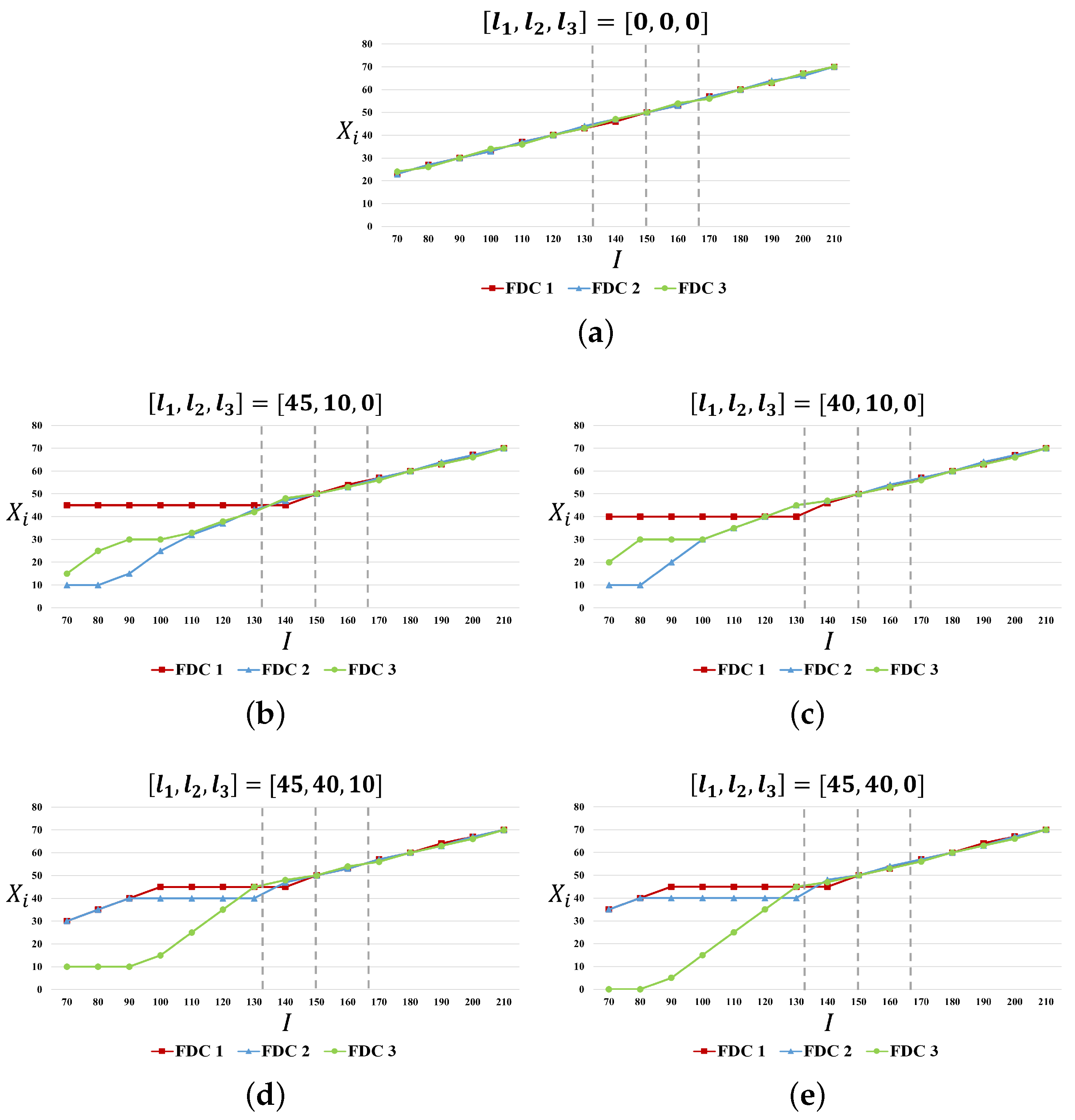
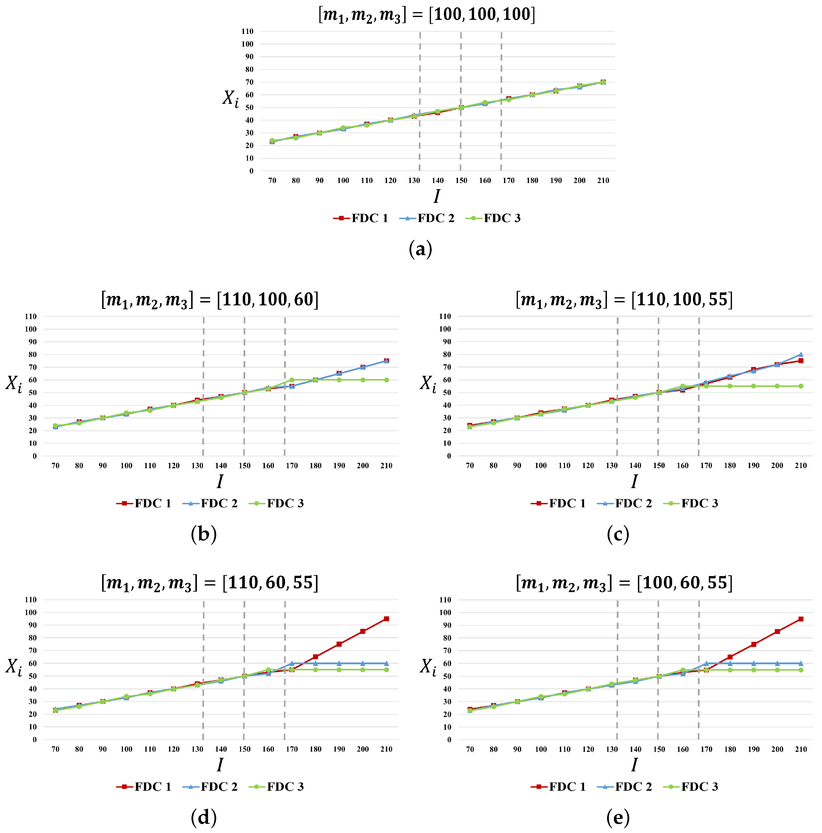
3.1.3. Experiment 3: Impact of Forecasted Bound on the Allocation Rule

In this experiment, we reveal the impact of the forecasted lower bound and upper bound of demand in each front-distribution-center-covered region on the allocation quantity to each front distribution center under different total available inventory conditions. Parameter settings of Experiment 3.a (Impact of Forecasted Lower Bound on the Allocation Rule) and Experiment 3.b (Impact of Forecasted Upper Bound on the Allocation Rule) are shown in

Table 4. Parameter setting of Experiment 3.a (impact of forecasted lower bound on the allocation rule).

	${\mu }_i$					${\sigma }_i^2$				$m_i$
FDC 1 †
FDC 2	50					25				100
FDC 3
$\lambda =0$
	$l_i$
FDC 1	0			45		40				45		45
FDC 2	0			10		10				40		40
FDC 3	0			0		0				10		0
I
70	80	90	100	110	120	130	140	150	160	170	180	190	200	210

† FDC: Front Distribution Center.

and

Table 5. Parameter setting of Experiment 3.b (impact of forecasted upper bound on the allocation rule).

	${\mu }_i$					${\sigma }_i^2$				$l_i$
FDC 1 †
FDC 2	50					25				0
FDC 3
$\lambda =0$
	$m_i$
FDC 1	100			110		110				110		100
FDC 2	100			100		100				60		60
FDC 3	100			60		55				55		55
I
70	80	90	100	110	120	130	140	150	160	170	180	190	200	210

† FDC: Front Distribution Center.

.

From Figure 4, we can find that, when the total available inventory is sufficient, the allocation quantity to each front distribution center is nearly the same. When the total available inventory is insufficient, there will be two situations. For the case where the lower bound is large enough (e.g., 40 or 45), higher priority will first be given to the region with the larger forecasted lower bound because, when the lower bound is tighter, the uncertainty will become smaller so as to ensure the basic sales volume and thereby stablize the sales in the future. For the case where the lower bound is small enough (e.g., 0 or 10), higher priority will first be given to the region with the forecasted lower bound to prepare for the potential high demand in the future because, if the same amounts of demands have been generated in the smallest interval (e.g., [lower bound, lower bound + 5]) in two regions with different lower bounds, due to the same overall forecasted mean and variance of demands in these two regions, the region with the smaller overall forecasted lower bound will have more chances to obtain higher demands in the future. In other words, the larger deviation between lower bound and mean brings larger risk, which will make the front distribution center in that region more likely to meet the potential high demand in the future. This discrepancy may even cause a phenomenon in which the allocation quantity to the region with the smallest lower bound overtakes the allocation quantity to the region with the largest lower bound when the total available inventory is very close to the sum of the forecasted means of demand in the three regions.

Under different total available inventory conditions, no matter whether the total available inventory is sufficient or insufficient, the impact of the forecasted upper bound of demand in each front-distribution-center-covered region on the allocation quantity to each front distribution center is similar to the impact of the forecasted lower bound, which has been already been thoroughly discussed in the last paragraph and thus will not be reiterated here. For details, please refer to Figure 5.

3.1.4. Experiment 4: Impact of Forecasted Variance on the Fulfillment Rates at a Fixed Inventory Level

In this experiment, we further investigate the impact of forecasted variance on fulfillment rates, including the front distribution center fulfillment rate and overall fulfillment rate. Here, we also use a network with one regional distribution center and three front distribution centers as the test environment. The parameters are given in

Table 6. Parameter setting of Experiment 4.

	Parameters
	$N=3,\lambda =1$
Algorithm 1
FDCs †	${\mu }_i\in \{0,5,\dots ,95,100\}$	$l_i=0$	$m_i=200$
	${\sigma }_i^2={({\alpha }_i{\mu }_i+{\beta }_i)}^2$	${\alpha }_i=0.2$	${\beta }_i=0$	$i=1,2,3$
RDC	${\mu }_R\in \{0,5,\dots ,95,100\}$	${\sigma }_R^2=100$	$l_R=0$	$m_R=200$
Algorithm 2
FDCs	${\mu }_i\in \{0,5,\dots ,95,100\}$	${\sigma }_i^2=100$	$l_i=0$	$m_i=200$	$i=1,2,3$
RDC	${\mu }_R\in \{0,5,\dots ,95,100\}$	${\sigma }_R^2=100$	$l_R=0$	$m_R=200$
Total Inventory	$I={\mu }_1+{\mu }_2+{\mu }_3+{\mu }_R+3({\sigma }_1+{\sigma }_2+{\sigma }_3+{\sigma }_R)$

† FDC: Front Distribution Center.

. In detail, we introduce two algorithms to reveal the impact of forecasted variance on fulfillment rates. The two algorithms are consistent in the forecasted mean, lower bound, and upper bound of demand in each front-distribution-center-covered region and the directly regional-distribution-center-covered region. The difference between the two algorithms mainly lies in that the forecasted variance of demand in each front-distribution-center-covered region is correlated to the forecasted mean as ${\sigma }_i^2={({\alpha }_i{\mu }_i+{\beta }_i)}^2$ in Algorithm 1, while the forecasted variance of demand remains constant at 100 in Algorithm 2 in order to reveal the impact of forecasted variance on fulfillment rates. For other parameters, we set the balance coefficient $\lambda =1$ and the total inventory level $I={\mu }_1+{\mu }_2+{\mu }_3+{\mu }_R+3({\sigma }_1+{\sigma }_2+{\sigma }_3+{\sigma }_R)$. This experiment is conducted in Python 3.8 with CPLEX 12.9 as the solver and run on a desktop featuring Intel Core i5-10210U CPU @ 1.6 GHz 2.11 GHz with 16 GB of RAM. In terms of specific steps, we input ${\mu }_i,{\alpha }_i,{\beta }_i,l_i,m_i,{\mu }_R,{\sigma }_R,l_R,m_R,\lambda ,I$ as shown in Table 6 to compute the optimal solution when testing Algorithm 1. However, when testing Algorithm 2, the input parameters are ${\mu }_i,{\sigma }_i,l_i,m_i,{\mu }_R,{\sigma }_R,l_R,m_R,\lambda ,I$, where the difference between the two algorithms mainly lies in that the forecasted variance of demand in each front-distribution-center-covered region is correlated to the forecasted mean in Algorithm 1 while the forecasted variance of demand remains constant in Algorithm 2. Under this configuration, the computational time to produce the optimal solution is 23.07 s on average. By contrast, the computational time of the frequently used SAA algorithm is 81.43 s on average, which is much larger (Sample Average Approximation algorithm—SAA algorithm for short—is a common approach for solving stochastic optimization problems that approximates the expected value in the objective function by using the average of a finite set of samples; by doing so, it transforms the stochastic optimization problem into a deterministic one that can be solved using standard optimization techniques [39]). At each inventory level, after solving the model, we randomly generate 1000-sample demand data from a Gaussian distribution (i.e., $d_R\sim N({\mu }_R,{\sigma }_R^2)$, $d_i\sim N({\mu }_i,{\sigma }_i^2)$, $i\in \mathcal{N}$). Finally, we subtract the fulfillment rates obtained in Algorithm 1 from the value obtained in Algorithm 2 to obtain the comparison result, as shown in Figure 6.

From Figure 6, we can discover that the front distribution center fulfillment rate under Algorithm 1 is lower and the overall fulfillment rate is higher than the ones under Algorithm 2 when the forecasted mean is relatively small. However, the results are exactly the opposite when the forecasted mean is relatively large. This phenomenon is caused by the following reason. When the forecasted mean is relatively small, the forecasted variance in Algorithm 1 is smaller than the one in Algorithm 2 since the forecasted variance of demand in each front-distribution-center-covered region is correlated to the forecasted mean as ${\sigma }_i^2={({\alpha }_i{\mu }_i+{\beta }_i)}^2$ in Algorithm 1 while it remains constant at 100 in Algorithm 2. The smaller forecasted variance of demand leads to fewer goods being allocated to the front distribution centers, eventually resulting in a lower front distribution center fulfillment rate and a higher overall fulfillment rate, and vice versa.

3.2. Experiment on Real Industry Data

Experiment 5: Impact of Forecasted Variance on the Fulfillment Rates at Different Inventory Levels.

In this experiment, our experimental data are based on the open-source dataset provided by Shanshu Operations (available at https://www.coap.online/competitions/1, accessed on 1 September 2024), which includes 18 DC regions, 77 different subcategories of products, and more than 880,000 historical sales data entries. We select four regions (DC 002, DC 004, DC 006, and DC 010) as our experimental area, where DC 002, DC 004, and DC 006 are the front distribution centers and DC 010 is the regional distribution center. Then, we compile the monthly sales data and choose the month with the highest sales volume (June 2020) and the lowest sales volume (March 2020) as the experimental time periods. For parameters, we conduct demand forecasting based on the historical sales data and set the balance coefficient $\lambda =1$. We still introduce two algorithms to reveal the impact of forecasted variance on fulfillment rates. The two algorithms are also consistent in the forecasted mean, lower bound, and upper bound of demand in each front-distribution-center-covered region and the directly regional-distribution-center-covered region. The difference between the two algorithms lies in that the forecasted variance of demand in each front-distribution-center-covered region and the directly regional-distribution-center-covered region is correlated to the forecasted mean as ${\sigma }_i^2={({\alpha }_i{\mu }_i+{\beta }_i)}^2$ and ${\sigma }_R^2={({\alpha }_R{\mu }_R+{\beta }_R)}^2$ in Algorithm 1, while it is set as a constant from historical sales data in Algorithm 2. For comparison, we subtract the fulfillment rates obtained in Algorithm 1 from the value obtained in Algorithm 2 to obtain the result in Figure 7.

Figure 7 shows the comparison of fulfillment rates under two algorithms at different inventory levels for March and June. Regardless of whether it is a high-sales month or a low-sales month, when the total inventory level in the entire region is relatively low, Algorithm 1 allocates fewer goods to the front distribution centers and correspondingly retains more inventory at the regional distribution center. This ensures that the overall fulfillment rate for the region is maintained at the necessary level, albeit at the cost of somewhat temporarily reducing the front distribution center fulfillment rate. Conversely, as the platform continues to replenish inventory to the region, causing the total inventory level in the entire region to gradually become relatively high, Algorithm 1 allocates more goods to the front distribution centers, thereby improving the front distribution center fulfillment rate. Moreover, such phenomena and the degree of variation are more pronounced in the low-sales month, rather than the high-sales month.

4. Discussion

The following discussion is based on the results data obtained by the numerical experiments introduced in the previous section.

4.1. Results

4.1.1. Impact of Forecasted Mean on the Allocation Rule

When the total available inventory is relatively insufficient ($I\le \widehat{\mu }-(n-1)\widehat{\sigma }={\displaystyle \frac{1}{n}}{\sum }_{i=1}^n{\mu }_i-(n-1)\sqrt{{\displaystyle \frac{1}{n}}{\sum }_{i=1}^n{\sigma }_i^2}$), the region with the smallest mean will have the largest volatility, which means the largest risk of unsalable commodities. Therefore, higher priority will be given to the region with larger forecasted mean of demand in order to ensure the basic sales volume as far as possible.

When the total available inventory is sufficient ($I\ge \widehat{\mu }-(n-1)\widehat{\sigma }={\displaystyle \frac{1}{n}}{\sum }_{i=1}^n{\mu }_i-(n-1)\sqrt{{\displaystyle \frac{1}{n}}{\sum }_{i=1}^n{\sigma }_i^2}$), the allocation quantity to each front distribution center is almost directly proportional to the forecasted mean of demand in each region.

4.1.2. Impact of Forecasted Variance on the Allocation Rule

When the total available inventory is insufficient ($I\le \widehat{\mu }={\displaystyle \frac{1}{n}}{\sum }_{i=1}^n{\mu }_i$), higher priority will be given to the region with the smaller forecasted variance of demand so as to ensure the basic sales volume with less uncertainty, thereby stablizing the future sales.

When the total available inventory is sufficient ($I\ge \widehat{\mu }={\displaystyle \frac{1}{n}}{\sum }_{i=1}^n{\mu }_i$), higher priority will be delivered to the region with the larger forecasted variance of demand so as to capture the risk.

4.1.3. Impact of Forecasted Bound on the Allocation Rule

When the total available inventory is insufficient ($I\le \widehat{\mu }-(n-1)\widehat{\sigma }={\displaystyle \frac{1}{n}}{\sum }_{i=1}^n{\mu }_i-(n-1)\sqrt{{\displaystyle \frac{1}{n}}{\sum }_{i=1}^n{\sigma }_i^2}$), there will be two situations. For the case in which the lower bound is large enough, higher priority will first be given to the region with larger forecasted lower bound because, when the lower bound is tighter, the uncertainty will become smaller so as to ensure the basic sales volume and thereby stablize the sales in the future. For the case in which the lower bound is small enough, higher priority will first be given to the region with smaller forecasted lower bound to prepare for the potential high demand in the future.

When the total available inventory is sufficient ($I\ge \widehat{\mu }={\displaystyle \frac{1}{n}}{\sum }_{i=1}^n{\mu }_i$), the allocation quantity to each front distribution center is nearly the same.

4.1.4. Impact of Forecasted Variance on the Fulfillment Rates at a Fixed Inventory Level

When the forecasted mean is relatively small, the smaller forecasted variance of demand leads to fewer goods being allocated to the front distribution centers, eventually resulting in a lower front distribution center fulfillment rate and a higher overall fulfillment rate, and vice versa.

4.1.5. Impact of Forecasted Variance on the Fulfillment Rates at Different Inventory Levels

When the total inventory level in the entire region is relatively low, fewer goods will be allocated to the front distribution centers, correspondingly retaining more inventory at the regional distribution center. This ensures that the overall fulfillment rate for the region is maintained at the necessary level, albeit at the cost of somewhat temporarily reducing the front distribution center fulfillment rate.

When the total inventory level in the entire region gradually become relatively high as the platform continues to replenish inventory to the region, more goods will be allocated to the front distribution centers, thereby improving the front distribution center fulfillment rate.

4.2. Limitation

However, the limitation of the algorithm lies in its inability to account for the correlations between different products. If one wishes to apply this algorithm under the situation where products are correlated, the case will be transformed into a semidefinite programming problem, which will require cooperation with some corresponding heuristic algorithms.

4.3. Extension

As an extension of this study, future studies could focus on how to apply the model and the correspoding algorithm from this study to the practical allocation and logistics networks in real-world supply chain scenarios to verify the robustness of our method in both daily sales and large-scale sales events. Moreover, the quantitative findings demonstrates that demand characteristics (such as the correlation between mean and variance) significantly influence allocation rules. This necessitates that E-commerce platforms establish reasonable product demand profiling systems. For instance, based on historical data clustering analysis, stock-keeping units can be categorized into stable (low variance), fluctuating (high variance), and seasonal (periodic variance) types, among others, with differentiated inventory strategies formulated accordingly. For example, for products with a positive correlation between mean and variance (such as new products), an aggressive forward stocking strategy should be adopted, while, for products with a negative correlation (such as end-of-life products), a conservative delayed replenishment strategy is more appropriate.

5. Conclusions

In this study, we improve a distributionally robust allocation model aimed at increasing front distribution centers’ fulfillment rates while also ensuring that the overall fulfillment rate for the region remains stable. Our approach incorporates a balance coefficient to achieve harmony between the front distribution center fulfillment rate and the regional fulfillment rate. To address demand uncertainty, we apply a moment-based distributionally robust optimization model. Then we reformulate this model into an equivalent mixed-integer linear programming model by segmenting the robust domain. Through numerical experiments and discussion, we comprehensively reveal the impact of moment information (including the mean, the variance, the lower bound, and the upper bound) in demand forecasting on the distributionally robust fulfillment rate improvement algorithm by discovering how demand forecasting influences the allocation rule and how forecasted variance influences the fulfillment rates at fixed or changing inventory levels. When the total available inventory is insufficient, higher priority will be given to the region with the smaller volatility of forecasted demand in order to ensure the basic sales volume as far as possible. In comparison, as the total available inventory gradually becomes sufficient, higher priority will be delivered to the region with the larger volatility of forecasted demand so as to prepare for the potential high demand in the future and thereby seize the opportunity to increase sales. As an extension of the present work, future studies could focus on two aspects. In terms of theoretical extensions, future studies could pay attention to the algorithm in situations where products are correlated. This case would be transformed into a semidefinite programming problem, which would require collaboration with corresponding heuristic algorithms. In terms of practical applications, future studies could concentrate on how to apply the algorithm developed in this study to real-world supply chain scenarios, such as allocation and logistics networks, to verify the robustness of the algorithm in both daily sales and large-scale sales events.

References

1. Lai, G.; Liu, H.; Xiao, W.; Zhao, X. “Fulfilled by amazon”: A strategic perspective of competition at the e-commerce platform. Manuf. Serv. Oper. Manag. 2022, 24, 1406–1420. [Google Scholar] [CrossRef]
2. Lei, Y.; Jasin, S.; Sinha, A. Joint dynamic pricing and order fulfillment for e-commerce retailers. Manuf. Serv. Oper. Manag. 2018, 20, 269–284. [Google Scholar] [CrossRef]
3. Das, S.; Ravi, R.; Sridhar, S. Order fulfillment under pick failure in omnichannel ship-from-store programs. Manuf. Serv. Oper. Manag. 2023, 25, 508–523. [Google Scholar] [CrossRef]
4. Miao, S.; Jasin, S.; Chao, X. Asymptotically optimal Lagrangian policies for multi-warehouse, multi-store systems with lost sales. Oper. Res. 2022, 70, 141–159. [Google Scholar] [CrossRef]
5. Dai, B.; Chen, H.; Li, Y.; Zhang, Y.; Wang, X.; Deng, Y. Inventory replenishment planning of a distribution system with storage capacity constraints and multi-channel order fulfilment. Omega 2021, 102, 102356. [Google Scholar] [CrossRef]
6. DeValve, L.; Wei, Y.; Wu, D.; Yuan, R. Understanding the value of fulfillment flexibility in an online retailing environment. Manuf. Serv. Oper. Manag. 2023, 25, 391–408. [Google Scholar] [CrossRef]
7. Bebitoğlu, B. Multi-Location Assortment Optimization Under Capacity Constraints. Ph.D. Thesis, Bilkent Universitesi, Ankara, Turkey, 2016. [Google Scholar]
8. Li, X.; Lin, H.; Liu, F. Shall We Only Store Popular Products? Warehouse Assortment Selection for E-Companies. Available online: https://ssrn.com/abstract=4212027 (accessed on 7 September 2022).
9. Lin, F.; Fang, X.; Gao, Z. Distributionally robust optimization: A review on theory and applications. Numer. Algebr. Control. Optim. 2022, 12, 159–212. [Google Scholar] [CrossRef]
10. Liu, Y.; Pichler, A.; Xu, H. Discrete approximation and quantification in distributionally robust optimization. Math. Oper. Res. 2019, 44, 19–37. [Google Scholar] [CrossRef]
11. Cheramin, M.; Cheng, J.; Jiang, R.; Pan, K. Computationally efficient approximations for distributionally robust optimization under moment and Wasserstein ambiguity. INFORMS J. Comput. 2022, 34, 1768–1794. [Google Scholar] [CrossRef]
12. Delage, E.; Ye, Y. Distributionally robust optimization under moment uncertainty with application to data-driven problems. Oper. Res. 2010, 58, 595–612. [Google Scholar] [CrossRef]
13. Hanasusanto, G.A.; Kuhn, D. Conic programming reformulations of two-stage distributionally robust linear programs over Wasserstein balls. Oper. Res. 2018, 66, 849–869. [Google Scholar] [CrossRef]
14. Liu, Y.; Meskarian, R.; Xu, H. Distributionally robust reward-risk ratio optimization with moment constraints. SIAM J. Optim. 2017, 27, 957–985. [Google Scholar]
15. Ardestani-Jaafari, A.; Delage, E. Robust optimization of sums of piecewise linear functions with application to inventory problems. Oper. Res. 2016, 64, 474–494. [Google Scholar]
16. Feng, H.; Feng, M.; Wang, Q.; Jin, Q.; Zhang, Y.; Cao, L.; Hao, X. Improving Front Distribution Center Fulfillment Rates: A Distributionally Robust Approach. Available online: https://ssrn.com/abstract=5054555 (accessed on 26 June 2024).
17. Liu, H.; Yu, Y.; Benjaafar, S.; Wang, H. Price-directed cost sharing and demand allocation among service providers with multiple demand sources and multiple facilities. Manuf. Serv. Oper. Manag. 2022, 24, 647–663. [Google Scholar]
18. Chen, Y.; Marković, N.; Ryzhov, I.O.; Schonfeld, P. Data-driven robust resource allocation with monotonic cost functions. Oper. Res. 2022, 70, 73–94. [Google Scholar]
19. Jasin, S.; Sinha, A. An LP-based correlated rounding scheme for multi-item e-commerce order fulfillment. Oper. Res. 2015, 63, 1336–1351. [Google Scholar]
20. Hwang, D.; Jaillet, P.; Manshadi, V. Online resource allocation under partially predictable demand. Oper. Res. 2021, 69, 895–915. [Google Scholar]
21. Angelus, A. A multiechelon inventory problem with secondary market sales. Manag. Sci. 2011, 57, 2145–2162. [Google Scholar] [CrossRef]
22. Klosterhalfen, S.T.; Minner, S.; Willems, S.P. Strategic safety stock placement in supply networks with static dual supply. Manuf. Serv. Oper. Manag. 2014, 16, 204–219. [Google Scholar]
23. Shang, K.H.; Tao, Z.; Zhou, S.X. Optimizing reorder intervals for two-echelon distribution systems with stochastic demand. Oper. Res. 2015, 63, 458–475. [Google Scholar]
24. Zhu, H.; Chen, Y.; Hu, M.; Yang, Y. Technical Note–A Simple Heuristic Policy for Stochastic Distribution Inventory Systems with Fixed Shipment Costs. Oper. Res. 2021, 69, 1651–1659. [Google Scholar] [CrossRef]
25. Ding, S.; Kaminsky, P.M. Centralized and decentralized warehouse logistics collaboration. Manuf. Serv. Oper. Manag. 2020, 22, 812–831. [Google Scholar] [CrossRef]
26. Drent, M.; Arts, J. Expediting in two-echelon spare parts inventory systems. Manuf. Serv. Oper. Manag. 2021, 23, 1431–1448. [Google Scholar] [CrossRef]
27. Shen, X.; Yu, Y.; Song, J.-S. Optimal policies for a multi-echelon inventory problem with service time target and expediting. Manuf. Serv. Oper. Manag. 2022, 24, 2310–2327. [Google Scholar] [CrossRef]
28. Zhen, L.; Wang, W.; Zhuge, D. Optimizing locations and scales of distribution centers under uncertainty. IEEE Trans. Syst. Man Cybern. Syst. 2016, 47, 2908–2919. [Google Scholar] [CrossRef]
29. Huang, J.; Shi, X. Solving the location problem of front distribution center for omni-channel retailing. Complex Intell. Syst. 2023, 9, 2237–2248. [Google Scholar] [CrossRef]
30. Shi, Y. Solving Inventory Assortment Problem by Utilizing Product Embedding. 2018. Available online: https://medium.com/jd-technology-blog/solving-inventory-assortment-problem-by-utilizing-product-embedding-807f992cb35a (accessed on 3 December 2018).
31. Axsäter, S. A new decision rule for lateral transshipments in inventory systems. Manag. Sci. 2003, 49, 1168–1179. [Google Scholar] [CrossRef]
32. Xu, P.J.; Allgor, R.; Graves, S.C. Benefits of reevaluating real-time order fulfillment decisions. Manuf. Serv. Oper. Manag. 2009, 11, 340–355. [Google Scholar] [CrossRef]
33. Govindan, K.; Jafarian, A.; Khodaverdi, R.; Devika, K. Two-echelon multiple-vehicle location-routing problem with time windows for optimization of sustainable supply chain network of perishable food. Int. J. Prod. Econ. 2014, 152, 9–28. [Google Scholar] [CrossRef]
34. Nagy, G.; Wassan, N.A.; Speranza, M.G.; Archetti, C. The vehicle routing problem with divisible deliveries and pickups. Transp. Sci. 2015, 49, 271–294. [Google Scholar] [CrossRef]
35. Franceschetti, A.; Honhon, D.; Laporte, G.; Van Woensel, T. A shortest-path algorithm for the departure time and speed optimization problem. Transp. Sci. 2018, 52, 756–768. [Google Scholar] [CrossRef]
36. Valipour, M.; Banihabib, M.E.; Behbahani, S.M.R. Parameters estimate of autoregressive moving average and autoregressive integrated moving average models and compare their ability for inflow forecasting. J. Math. Stat. 2012, 8, 330–338. [Google Scholar]
37. Natarajan, K.; Sim, M.; Uichanco, J. Tractable robust expected utility and risk models for portfolio optimization. Math. Financ. 2010, 20, 695–731. [Google Scholar]
38. Nickel, S.; Steinhardt, C.; Schlenker, H.; Burkart, W. Decision Optimization with IBM ILOG CPLEX Optimization Studio; Springer: Berlin/Heidelberg, Germany, 2022. [Google Scholar]
39. Kim, S.; Pasupathy, R.; Henderson, S.G. A guide to sample average approximation. In Handbook of Simulation Optimization; Springer: Berlin/Heidelberg, Germany, 2015; pp. 207–243. [Google Scholar]
Figure 1. Flow chart of the distributionally robust allocation algorithm.
Mathematics 13 01172 g001
Figure 2. Comparisons of allocation quantities to front distribution centers under different forecasted means. (a) Allocation quantities under [ μ 1 , μ 2 , μ 3 ] = [ 50 , 50 , 50 ] ; (b) Allocation quantities under [ μ 1 , μ 2 , μ 3 ] = [ 60 , 50 , 40 ] ; (c) Allocation quantities under [ μ 1 , μ 2 , μ 3 ] = [ 80 , 50 , 20 ] ; (d) Allocation quantities under [ μ 1 , μ 2 , μ 3 ] = [ 80 , 50 , 40 ] ; (e) Allocation quantities under [ μ 1 , μ 2 , μ 3 ] = [ 60 , 50 , 20 ] . (FDC: Front Distribution Center, X i : Allocation Quantity, I: Total Available Inventory, μ i : Forecasted Mean).
Mathematics 13 01172 g002
Figure 3. Comparisons of allocation quantities to front distribution centers under different forecasted variances. (a) Allocation quantities under [ σ 1 2 , σ 2 2 , σ 3 2 ] = [ 25 , 25 , 25 ] ; (b) Allocation quantities under [ σ 1 2 , σ 2 2 , σ 3 2 ] = [ 100 , 25 , 1 ] ; (c) Allocation quantities under [ σ 1 2 , σ 2 2 , σ 3 2 ] = [ 400 , 25 , 1 ] ; (d) Allocation quantities under [ σ 1 2 , σ 2 2 , σ 3 2 ] = [ 400 , 100 , 1 ] ; (e) Allocation quantities under [ σ 1 2 , σ 2 2 , σ 3 2 ] = [ 400 , 100 , 25 ] . (FDC: Front Distribution Center, X i : Allocation Quantity, I: Total Available Inventory, σ i 2 : Forecasted Variance).
Mathematics 13 01172 g003
Figure 4. Comparisons of allocation quantities to front distribution centers under different forecasted lower bounds. (a) Allocation quantities under [ l 1 , l 2 , l 3 ] = [ 0 , 0 , 0 ] ; (b) Allocation quantities under [ l 1 , l 2 , l 3 ] = [ 45 , 10 , 0 ] ; (c) Allocation quantities under [ l 1 , l 2 , l 3 ] = [ 40 , 10 , 0 ] ; (d) Allocation quantities under [ l 1 , l 2 , l 3 ] = [ 45 , 40 , 10 ] ; (e) Allocation quantities under [ l 1 , l 2 , l 3 ] = [ 45 , 40 , 0 ] . (FDC: Front Distribution Center, X i : Allocation Quantity, I: Total Available Inventory, l i : Forecasted Lower Bound).
Mathematics 13 01172 g004
Figure 5. Comparisons of allocation quantities to front distribution centers under different forecasted upper bounds. (a) Allocation quantities under [ m 1 , m 2 , m 3 ] = [ 100 , 100 , 100 ] ; (b) Allocation quantities under [ m 1 , m 2 , m 3 ] = [ 110 , 100 , 60 ] ; (c) Allocation quantities under [ m 1 , m 2 , m 3 ] = [ 110 , 100 , 55 ] ; (d) Allocation quantities under [ m 1 , m 2 , m 3 ] = [ 110 , 60 , 55 ] ; (e) Allocation quantities under [ m 1 , m 2 , m 3 ] = [ 100 , 60 , 55 ] . (FDC: Front Distribution Center, X i : Allocation Quantity, I: Total Available Inventory, m i : Forecasted Upper Bound).
Mathematics 13 01172 g005
Figure 6. Comparison of fulfillment rates under two algorithms at fixed inventory levels. (FDC: Front Distribution Center, I: Total Available Inventory).
Mathematics 13 01172 g006
Figure 7. Comparison of fulfillment rates under two algorithms at different inventory levels. (FDC: Front Distribution Center).
Mathematics 13 01172 g007