
Integrated Neural Network for Ordering Optimization with Intertemporal-Dependent Demand and External Features


Abstract
1. Introduction
2. Literature Review
3. Methodology
3.1. Problem Description
3.2. Custom Hybrid Neural Network
3.2.1. Custom Newsvendor Loss Function
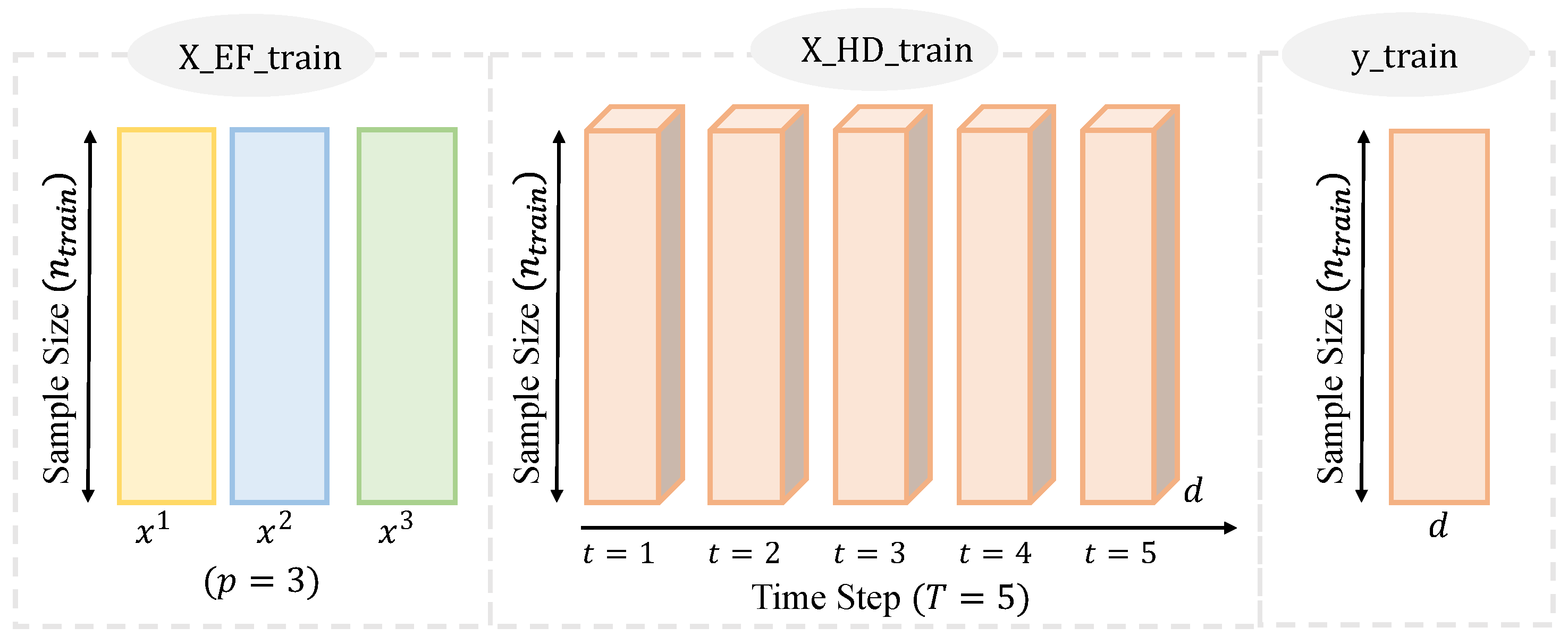
3.2.2. Hybrid Neural Network Structure
3.2.3. Performance Metrics
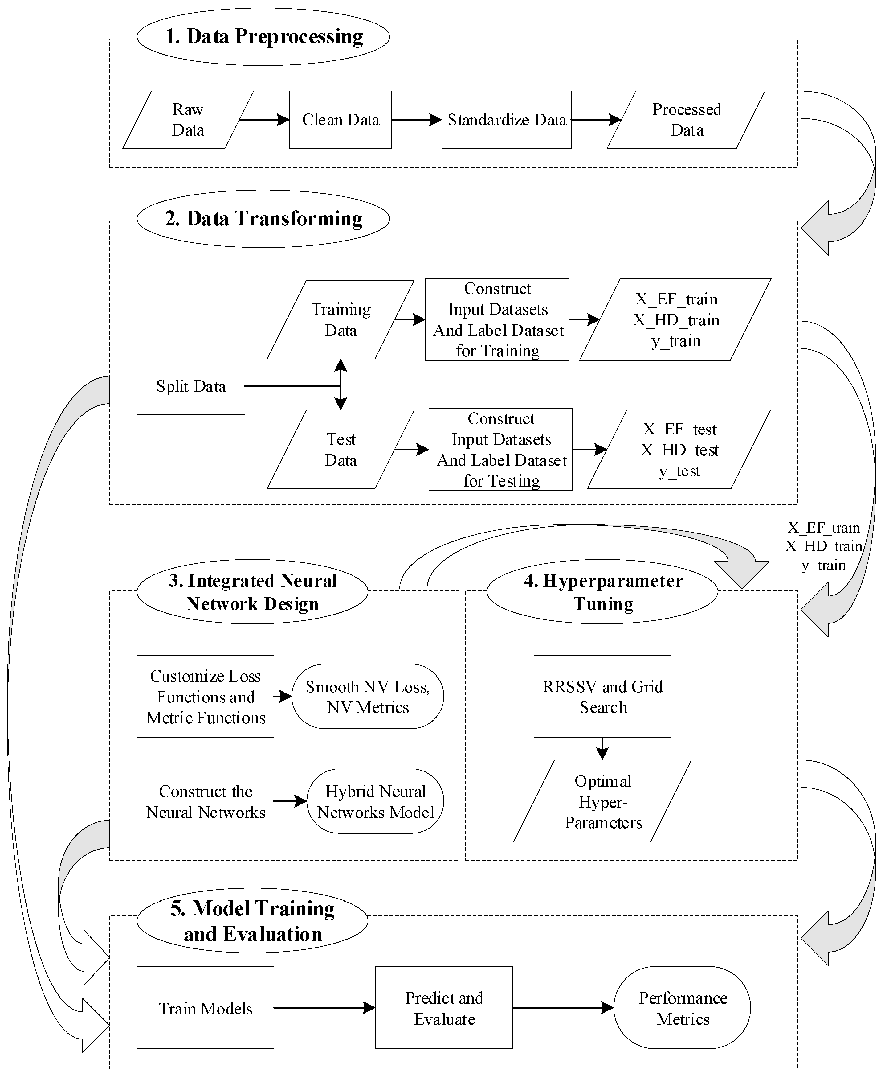
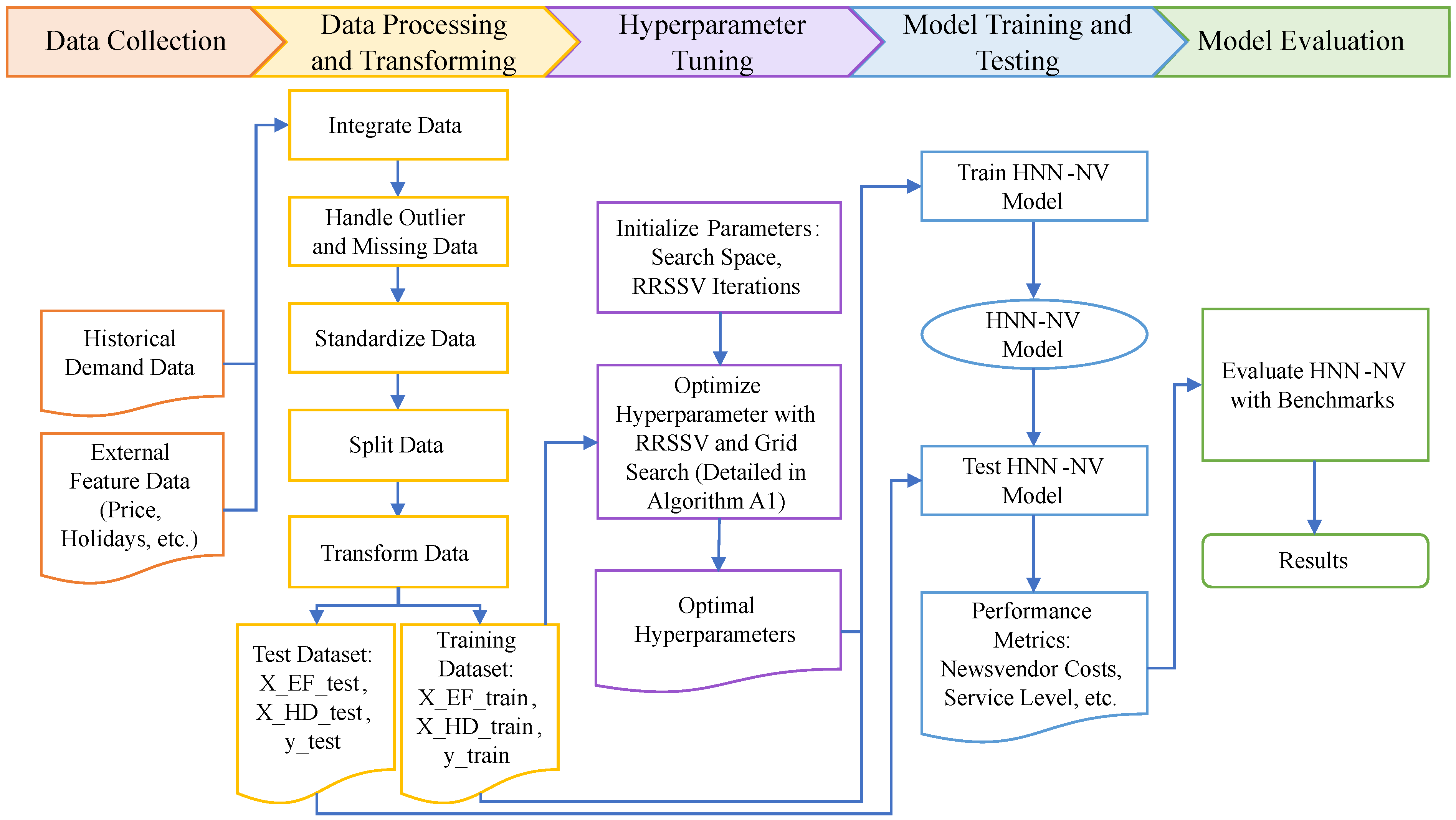
3.3. Integrated Newsvendor Framework
- The entire training dataset, consisting of , is randomly partitioned into the training and validation set K times (e.g., five times). These partitions are denoted as for the training sets and for the validation sets, where .
- For each combination of the hyperparameters within the specified search space, the following occurs:
- (a)
- For each of the K random split datasets, the model is trained on the respective training set, , and the average newsvendor cost is computed as the evaluation metric on the validation set, .
- (b)
- The average performance metric across the K splits is then calculated.
- The hyperparameter combination that yields the lowest average evaluation metric across the K splits is selected as the optimal set of hyperparameters.
4. Case Study: Order Quantity Optimization of Vegetables
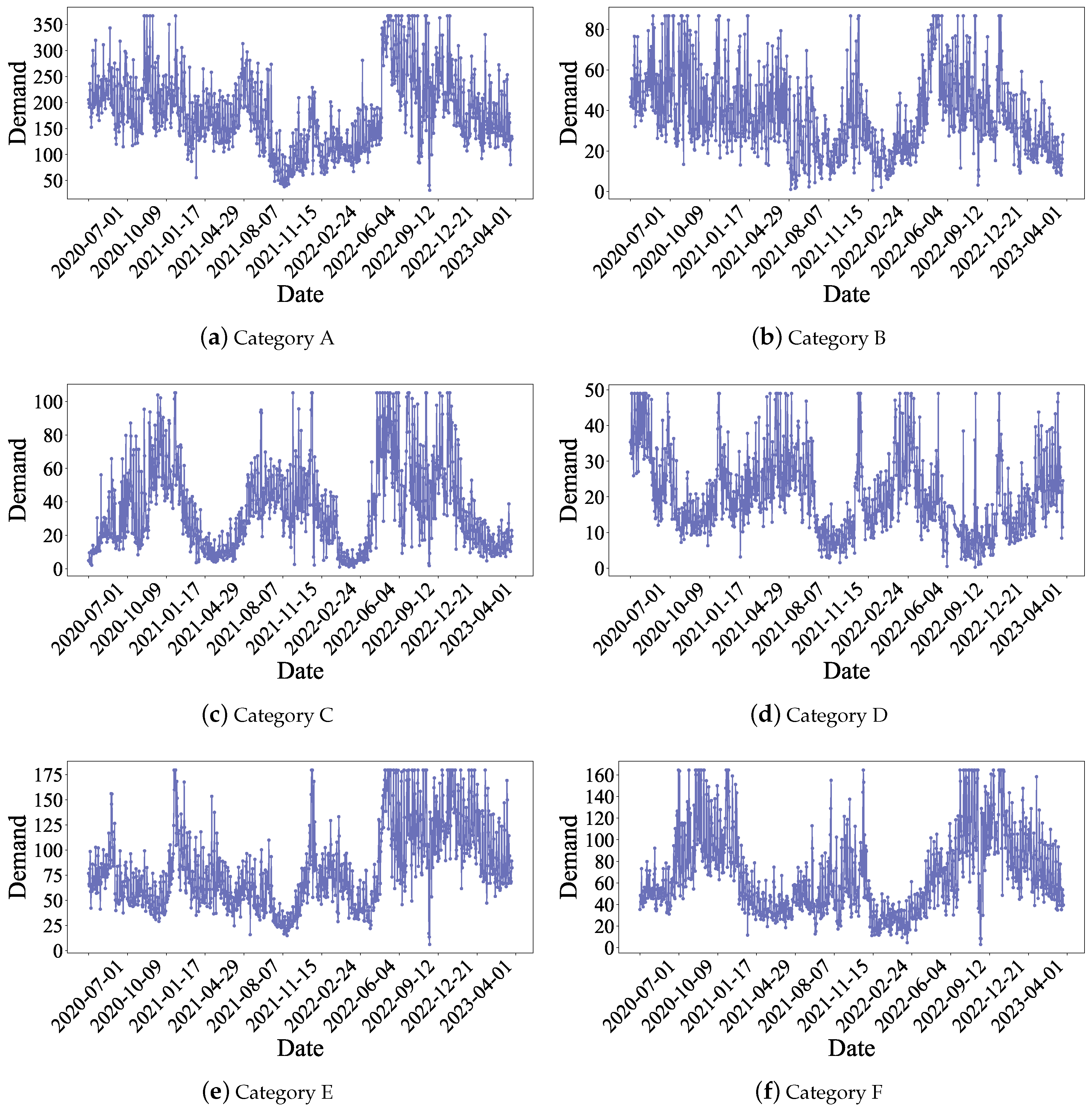
4.1. Data
4.2. Benchmark Methods
4.3. Experimental Setup and Hyperparameter Optimization
5. Results and Discussion
5.1. Results
5.2. Discussion
6. Conclusions
Author Contributions
Funding
Data Availability Statement
Conflicts of Interest
Appendix A. Supplementary Material for Case Study
Appendix A.1. Hyperparameter Tuning for HNN-NV
| Algorithm A1 Hyperparameter optimization with RRSSV and grid search for HNN-NV | ||
| Input: X_EF_train: Input dataset for Input_EF layer | ||
| 1: | X_HD_train: Input dataset for Input_HD layer | |
| 2: | y_train: Label dataset | |
| 3: | α: Cost coefficient in Equation (5) | |
| 4: | K: RRSSV iterations | |
| 5: | ρ: Ratio of validation set | |
| 6: | : Search space for hyperparameters | |
| 7: | : Initial hyperparameter configuration | |
| Output: : Optimal hyperparameter configuration | ||
| 8: | : Minimal average validation cost | |
| 9: | // Define hyperparameter space | |
| 10: | // B: Batch size; : Number of units in LSTM_layer; | |
| 11: | // : Number of units in Dense_layer_EF; : Number of units in Dense_layer | |
| 12: | ||
| 13: | // Initialize optimal records | |
| 14: | , | |
| 15: | // Grid search loop | |
| 16: | for all do | |
| 17: | ▹ Current parameter configuration | |
| 18: | ▹ Cost record set | |
| 19: | // RRSSV iteration | |
| 20: | for k = 1 to K do | |
| 21: | , , , (, , ) | |
| ← GenerateSplit(, , , , k) | ||
| 22: | ← TrainValidate(, , , , | |
| , , , ) | ▹ Model training & validation | |
| 23: | ▹ Cost record | |
| 24: | ← Mean() | ▹ Compute mean cost |
| 25: | if then | |
| 26: | ||
| 27: | ||
| Key Function Specifications: | ||
| - GenerateSplit: Generates random training/validation split | ||
| - TrainValidate: Performs the following operations: | ||
| 1. Build the integrated Neural Network network: | ||
| • LSTM_layer: units | ||
| • Dense_layer_EF: units | ||
| • Dense_layer: units | ||
| • Loss function: Equation (5) | ||
| 2. Train in train set (, , ) with batch size b for a maximum of 500 iterations or early stopping with no loss improvement | ||
| 3. Compute newsvendor cost C in validation set (, , ) with Equation (7) | ||
Appendix A.2. Comparative Results with Traditional Neural Network-Based Method

| α | HNN-NV | NN-NV | ||
|---|---|---|---|---|
| Mean (SEM) | Mean (SEM) | ΔNVC | t-Test p-Value | |
| 0.3 | 42.54 (1.76) | 67.97 (2.56) | 25.43 | 0.000 **** |
| 0.4 | 47.96 (2.06) | 79.72 (3.18) | 31.77 | 0.000 **** |
| 0.5 | 49.24 (2.22) | 88.84 (3.89) | 39.6 | 0.000 **** |
| 0.6 | 49.97 (2.34) | 91.29 (4.17) | 41.32 | 0.000 **** |
| 0.7 | 46.63 (2.29) | 89.09 (4.38) | 42.46 | 0.000 **** |
| 0.8 | 39.35 (1.73) | 76.46 (4.21) | 37.11 | 0.000 **** |
References
- Zipkin, P.H. Foundations of Inventory Management; Irwin/McGraw-Hill: New York, NY, USA, 2000. [Google Scholar]
- Porteus, E.L. Foundations of Stochastic Inventory Theory; Stanford University Press: Redwood City, CA, USA, 2002. [Google Scholar]
- Scarf, H.E. A min-max solution of an inventory problem. In Studies in the Mathematical Theory of Inventory and Production; Arrow, K.J., Karlin, S., Scarf, H.E., Eds.; Stanford University Press: Redwood City, CA, USA, 1958; pp. 201–209. [Google Scholar]
- Ban, G.Y.; Rudin, C. The big data newsvendor: Practical insights from machine learning. Oper. Res. 2019, 67, 90–108. [Google Scholar] [CrossRef]
- Huber, J.; Müller, S.; Fleischmann, M.; Stuckenschmidt, H. A data-driven newsvendor problem: From data to decision. Eur. J. Oper. Res. 2019, 278, 904–915. [Google Scholar] [CrossRef]
- Oroojlooyjadid, A.; Snyder, L.V.; Takáč, M. Applying deep learning to the newsvendor problem. IISE Trans. 2020, 52, 444–463. [Google Scholar]
- Besbes, O.; Mouchtaki, O. How big should your data really be? Data-driven newsvendor: Learning one sample at a time. Manag. Sci. 2023, 69, 5848–5865. [Google Scholar] [CrossRef]
- Ren, K.; Bidkhori, H.; Shen, Z.J.M. Data-driven inventory policy: Learning from sequentially observed non-stationary data. Omega 2024, 123, 102942. [Google Scholar] [CrossRef]
- Qi, M.; Shen, Z.J.M.; Zheng, Z. Learning newsvendor problems with intertemporal dependence and moderate non-stationarities. Prod. Oper. Manag. 2024, 33, 1196–1213. [Google Scholar]
- Qi, M.; Shi, Y.; Qi, Y.; Ma, C.; Yuan, R.; Wu, D.; Shen, Z.J.M. A practical end-to-end inventory management model with deep learning. Manag. Sci. 2023, 69, 759–773. [Google Scholar] [CrossRef]
- Bertsimas, D.; Kallus, N. From Predictive to Prescriptive Analytics. Manag. Sci. 2020, 66, 1025–1044. [Google Scholar] [CrossRef]
- Hochreiter, S.; Schmidhuber, J. Long short-term memory. Neural Comput. 1997, 9, 1735–1780. [Google Scholar] [CrossRef]
- Wang, Y.; Shen, Y.; Mao, S.; Chen, X.; Zou, H. LASSO and LSTM integrated temporal model for short-term solar intensity forecasting. IEEE Internet Things J. 2018, 6, 2933–2944. [Google Scholar] [CrossRef]
- Kim, M.; Lee, J.; Lee, C.; Jeong, J. Framework of 2D KDE and LSTM-based forecasting for cost effective inventory management in smart manufacturing. Appl. Sci. 2022, 12, 2380. [Google Scholar] [CrossRef]
- Ping, H.; Li, Z.; Shen, X.; Sun, H. Optimization of vegetable restocking and pricing strategies for innovating supermarket operations utilizing a combination of ARIMA, LSTM, and FP-growth algorithms. Mathematics 2024, 12, 1054. [Google Scholar] [CrossRef]
- Punia, S.; Nikolopoulos, K.; Singh, S.P.; Madaan, J.K.; Litsiou, K. Deep learning with long-short-term memory networks and random forests for demand forecasting in multi-channel retail. Int. J. Prod. Res. 2020, 58, 4964–4979. [Google Scholar]
- Qin, Y.; Wang, R.; Vakharia, A.J.; Chen, Y.; Seref, M.M.H. The newsvendor problem: Review and directions for future research. Eur. J. Oper. Res. 2011, 213, 361–374. [Google Scholar]
- DeYong, G.D. The price-setting newsvendor: Review and extensions. Int. J. Prod. Res. 2020, 58, 1776–1804. [Google Scholar]
- Levi, R.; Roundy, R.O.; Shmoys, D.B. Provably near-optimal sampling-based policies for stochastic inventory control models. Math. Oper. Res. 2007, 32, 821–839. [Google Scholar]
- Levi, R.; Perakis, G.; Uichanco, J. The data-driven newsvendor problem: New bounds and insights. Oper. Res. 2015, 63, 1294–1306. [Google Scholar] [CrossRef]
- Lin, M.; Huh, W.T.; Krishnan, H.; Uichanco, J. Technical note—Data-driven newsvendor problem: Performance of the sample average approximation. Oper. Res. 2022, 70, 1996–2012. [Google Scholar]
- Beutel, A.L.; Minner, S. Safety stock planning under causal demand forecasting. Int. J. Prod. Econ. 2012, 140, 637–645. [Google Scholar]
- Zhang, Y.; Gao, J. Assessing the performance of deep learning algorithms for newsvendor problem. In Proceedings of the Neural Information Processing: 24th International Conference (ICONIP), Guangzhou, China, 14–18 November 2017; Part I 24. pp. 912–921. [Google Scholar]
- Trapero, J.R.; Cardós, M.; Kourentzes, N. Empirical safety stock estimation based on kernel and GARCH models. Omega 2019, 84, 199–211. [Google Scholar]
- Alwan, L.C.; Xu, M.; Yao, D.Q.; Yue, X. The dynamic newsvendor model with correlated demand. Decis. Sci. 2016, 47, 11–30. [Google Scholar] [CrossRef]
- Carrizosa, E.; Olivares-Nadal, A.V.; Ramírez-Cobo, P. Robust newsvendor problem with autoregressive demand. Comput. Oper. Res. 2016, 68, 123–133. [Google Scholar]
- Lugosi, G.; Markakis, M.G.; Neu, G. On the hardness of learning from censored and nonstationary demand. INFORMS J. Optim. 2024, 6, 63–83. [Google Scholar] [CrossRef]
- Kilic, O.A.; Tarim, S.A. A simple heuristic for computing non-stationary inventory policies based on function approximation. Eur. J. Oper. Res. 2024, 316, 899–905. [Google Scholar]
- Cao, Y.; Shen, Z.J.M. Quantile forecasting and data-driven inventory management under nonstationary demand. Oper. Res. Lett. 2019, 47, 465–472. [Google Scholar] [CrossRef]
- Dehaybe, H.; Catanzaro, D.; Chevalier, P. Deep Reinforcement Learning for inventory optimization with non-stationary uncertain demand. Eur. J. Oper. Res. 2024, 314, 433–445. [Google Scholar]
- Choi, T.M.; Wen, X.; Sun, X.; Chung, S.H. The mean-variance approach for global supply chain risk analysis with air logistics in the blockchain technology era. Transp. Res. Part E: Logist. Transp. Rev. 2019, 127, 178–191. [Google Scholar]
- Loureiro, A.L.D.; Miguéis, V.L.; da Silva, L.F.M. Exploring the use of deep neural networks for sales forecasting in fashion retail. Decis. Support Syst. 2018, 114, 81–93. [Google Scholar]
- Cao, W.; Liu, H.; Zhang, X.; Zeng, Y. Residential load forecasting based on long short-term memory, considering temporal local attention. Sustainability 2024, 16, 11252. [Google Scholar] [CrossRef]
- Abbasimehr, H.; Shabani, M.; Yousefi, M. An optimized model using LSTM network for demand forecasting. Comput. Ind. Eng. 2020, 43, 106435. [Google Scholar] [CrossRef]
- Niu, T.; Zhang, H.; Yan, X.; Miao, Q. Intricate supply chain demand forecasting based on graph convolution network. Sustainability 2024, 16, 9608. [Google Scholar] [CrossRef]
- Nasseri, M.; Falatouri, T.; Brandtner, P.; Darbanian, F. Applying machine learning in retail demand prediction—A comparison of tree-based ensembles and long short-term memory-based deep learning. Appl. Sci. 2023, 13, 11112. [Google Scholar] [CrossRef]
- Hurtado-Mora, H.A.; García-Ruiz, A.H.; Pichardo-Ramírez, R.; González-del-Ángel, L.J.; HerreraBarajas, L.A. Sales forecasting with LSTM, custom loss function, and hyperparameter optimization: A case study. Appl. Sci. 2024, 14, 9957. [Google Scholar] [CrossRef]
- Koenker, R.; Bassett, G., Jr. Regression quantiles. Econometrica 1978, 46, 33–50. [Google Scholar] [CrossRef]
- Robbins, H.; Monro, S. A stochastic approximation method. Ann. Math. Stat. 1951, 22, 400–407. [Google Scholar]
- Cannon, A.J. Quantile regression neural networks: Implementation in R and application to precipitation downscaling. Comput. Geosci. 2011, 37, 1277–1284. [Google Scholar]
- Chen, C. A finite smoothing algorithm for quantile regression. J. Comput. Graph. Stat. 2007, 16, 136–164. [Google Scholar]
- Goltsos, T.E.; Syntetos, A.A.; Glock, C.H.; Ioannou, G. Inventory-forecasting: Mind the gap. Eur. J. Oper. Res. 2022, 299, 397–419. [Google Scholar]


| External Feature | Description |
|---|---|
| Maximum price in the group by date and vegetable category | |
| Minimum price in the group by date and vegetable category | |
| Weighted average price in the group by date and vegetable category | |
| Percentage of discount promotions within the group by date and vegetable category | |
| Holiday |
| Date | d | d (Scaled) | |||||
|---|---|---|---|---|---|---|---|
| 2020-07-01 | 205.39 | 0.5191 | 0.0989 | 0.6596 | 0.5962 | 0.1356 | 0 |
| 2020-07-02 | 198.35 | 0.4981 | 0.0989 | 0.1277 | 0.5714 | 0.1516 | 0 |
| 2020-07-03 | 190.77 | 0.4755 | 0.0989 | 0.7447 | 0.5974 | 0.0604 | 0 |
| 2020-07-04 | 236.58 | 0.6121 | 0.0989 | 0.7447 | 0.6505 | 0.0108 | 0 |
| 2020-07-05 | 223.91 | 0.5743 | 0.0555 | 0.8298 | 0.5620 | 0.0223 | 0 |
| 2020-07-06 | 195.73 | 0.4903 | 0.0989 | 0.8298 | 0.6434 | 0.0675 | 0 |
| 2020-07-07 | 172.06 | 0.4197 | 0.0989 | 0.7234 | 0.6399 | 0.1185 | 0 |
| 2020-07-08 | 152.57 | 0.3616 | 0.1162 | 0.8298 | 0.6600 | 0.1459 | 0 |
| 2020-07-09 | 187.45 | 0.4656 | 0.1162 | 0.0426 | 0.6116 | 0.0048 | 0 |
| 2020-07-10 | 179.84 | 0.4429 | 0.1162 | 0.6596 | 0.5891 | 0.2413 | 0 |
| HNN-NV | HNN-SEO | HNN-MSE | LSTM-NV | |
|---|---|---|---|---|
| 0.3 | 18.68% | 16.38% | 0.00% | 12.41% |
| 0.4 | 9.62% | 4.86% | 2.33% | 0.00% |
| 0.5 | 10.16% | 2.88% | 6.33% | 0.00% |
| 0.6 | 12.73% | 8.32% | 11.18% | 0.00% |
| 0.7 | 9.68% | 5.75% | 2.42% | 0.00% |
| 0.8 | 21.14% | 17.69% | 0.00% | 10.90% |
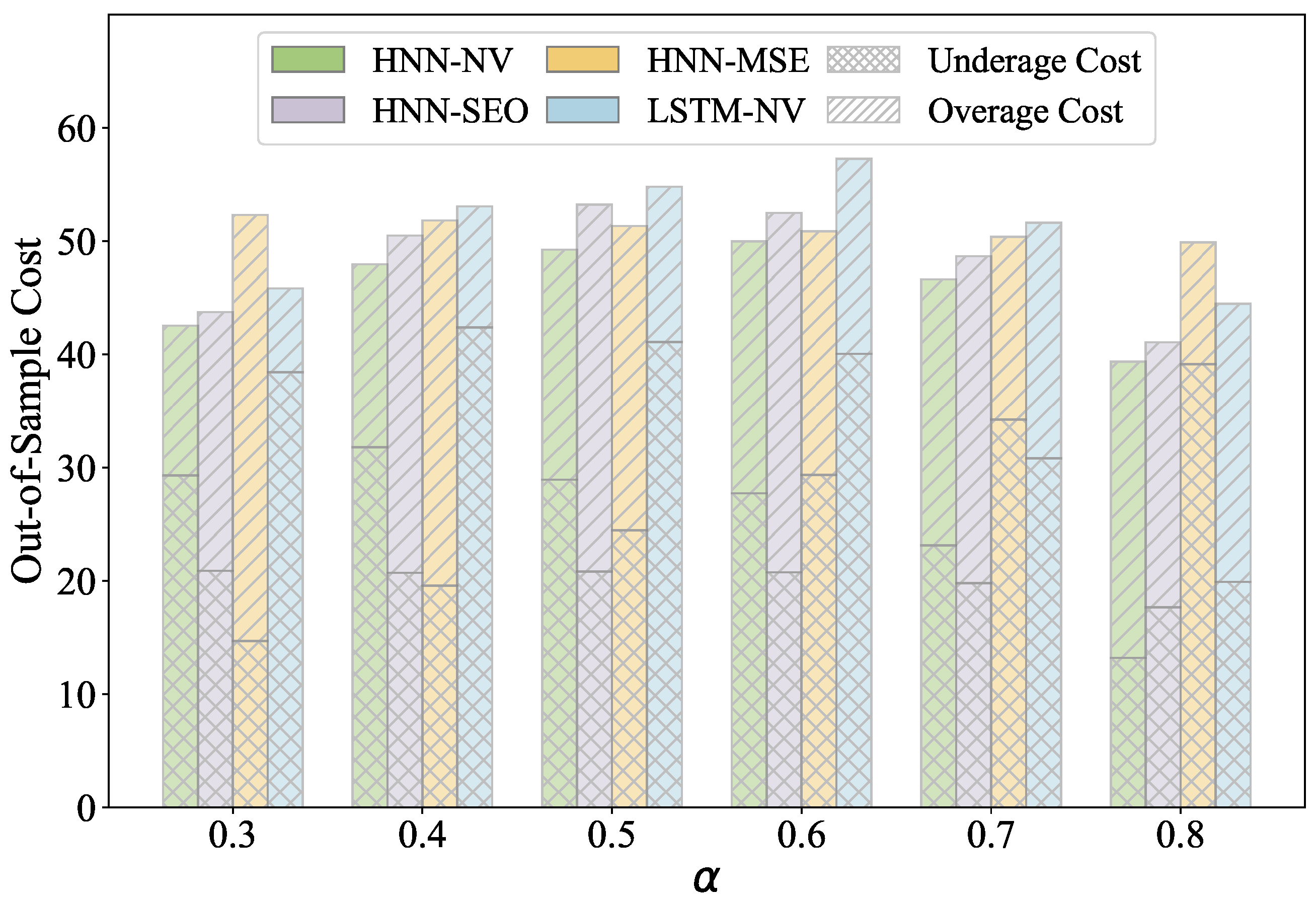
| α | HNN-NV | HNN-SEO | HNN-MSE | LSTM-NV | ||||||
|---|---|---|---|---|---|---|---|---|---|---|
| Mean (SEM) | Mean (SEM) | ΔNVC | t-Test p-Value | Mean (SEM) | ΔNVC | t-Test p-Value | Mean (SEM) | ΔNVC | t-Test p-Value | |
| 0.3 | 42.54 (1.76) | 43.74 (1.89) | 1.20 | 0.296 | 52.31 (2.22) | 9.77 | 0.000 **** | 45.82 (1.95) | 3.28 | 0.002 *** |
| 0.4 | 47.96 (2.06) | 50.48 (2.00) | 2.53 | 0.054 * | 51.83 (2.02) | 3.87 | 0.008 *** | 53.06 (2.4) | 5.11 | 0.000 **** |
| 0.5 | 49.24 (2.22) | 53.23 (2.02) | 3.99 | 0.000 **** | 51.34 (2.08) | 2.1 | 0.001 *** | 54.81 (2.65) | 5.57 | 0.000 **** |
| 0.6 | 49.97 (2.34) | 52.5 (2.01) | 2.52 | 0.008 *** | 50.86 (2.4) | 0.89 | 0.031 ** | 57.27 (2.87) | 7.29 | 0.000 **** |
| 0.7 | 46.63 (2.29) | 48.66 (2.01) | 2.03 | 0.008 *** | 50.38 (2.88) | 3.75 | 0.001 *** | 51.63 (2.58) | 5 | 0.000 **** |
| 0.8 | 39.35 (1.73) | 41.07 (1.98) | 1.72 | 0.018 ** | 49.89 (3.45) | 10.55 | 0.000 **** | 44.46 (2.00) | 5.11 | 0.000 **** |
| TSL 1 (α) | HNN-NV | HNN-SEO | HNN-MSE | LSTM-NV | ||||
|---|---|---|---|---|---|---|---|---|
| RSL 2 | ΔSL 3 | RSL | ΔSL | RSL | ΔSL | RSL | ΔSL | |
| 0.3 | 0.32 | 0.02 | 0.42 | 0.12 | 0.60 | 0.30 | 0.25 | −0.05 |
| 0.4 | 0.39 | −0.01 | 0.55 | 0.15 | 0.60 | 0.20 | 0.37 | −0.03 |
| 0.5 | 0.52 | 0.02 | 0.64 | 0.14 | 0.60 | 0.10 | 0.45 | −0.05 |
| 0.6 | 0.61 | 0.01 | 0.71 | 0.11 | 0.60 | 0.00 | 0.55 | −0.05 |
| 0.7 | 0.71 | 0.01 | 0.75 | 0.05 | 0.60 | −0.10 | 0.68 | −0.02 |
| 0.8 | 0.84 | 0.04 | 0.80 | 0.00 | 0.60 | −0.20 | 0.78 | −0.02 |
Disclaimer/Publisher’s Note: The statements, opinions and data contained in all publications are solely those of the individual author(s) and contributor(s) and not of MDPI and/or the editor(s). MDPI and/or the editor(s) disclaim responsibility for any injury to people or property resulting from any ideas, methods, instructions or products referred to in the content. |
© 2025 by the authors. Licensee MDPI, Basel, Switzerland. This article is an open access article distributed under the terms and conditions of the Creative Commons Attribution (CC BY) license (https://creativecommons.org/licenses/by/4.0/).
Share and Cite
Chen, M.; Fu, K. Integrated Neural Network for Ordering Optimization with Intertemporal-Dependent Demand and External Features. Mathematics 2025, 13, 1149. https://doi.org/10.3390/math13071149
Chen M, Fu K. Integrated Neural Network for Ordering Optimization with Intertemporal-Dependent Demand and External Features. Mathematics. 2025; 13(7):1149. https://doi.org/10.3390/math13071149
Chicago/Turabian StyleChen, Minxia, and Ke Fu. 2025. "Integrated Neural Network for Ordering Optimization with Intertemporal-Dependent Demand and External Features" Mathematics 13, no. 7: 1149. https://doi.org/10.3390/math13071149
APA StyleChen, M., & Fu, K. (2025). Integrated Neural Network for Ordering Optimization with Intertemporal-Dependent Demand and External Features. Mathematics, 13(7), 1149. https://doi.org/10.3390/math13071149