1. Introduction
Inflation forecasting plays a crucial role in making wise financial decisions. Nominal phrases are often used in debt, employment, tenancy, and sales contracts. For this reason, politicians, corporations, and families need to be able to foresee inflation. Furthermore, inflation projections are a critical instrument that central banks use to direct their monetary policy actions, shape inflation expectations, and advance economic stability in general. This approach helps the central bank while enabling people and companies to make better financial decisions [
1,
2,
3,
4,
5].
In the past, numerous researchers projected the inflation rate through various forecasting models. For example, the study discussed in [
6] analyzed how machineearning (ML) techniques enhanced inflation predictions in Brazil. By examining a comprehensive dataset and utilizing 50 distinct forecasting methods, the research showed that ML techniques often outperformed traditional econometric models the regarding mean-squared error. Furthermore, the findings emphasized the existence of nonlinearities in inflation dynamics, indicating that these methods were beneficial for macroeconomic forecasts in Brazil. Likewise, the research outlined in [
7] investigated the influence of investor attention on comprehending and predicting inflation, using methods such as Granger causality tests, vector autoregression models, inear models, and various statistical indicators. The results suggested that investor attention was a Granger cause of inflation and negatively impacted it. Models that included investor attention demonstrated superior forecasting performance compared to standard benchmark models. Moreover, the paper indicated that investor attention influenced inflation through its effect on inflation expectations, underscoring its importance within macroeconomic studies.
Conversely, the research described in [
8] ooked into machineearning in conjunction with traditional forecasting techniques for predicting inflation in developing countries. It evaluated whether machineearning methods were more effective than conventional approaches, noting that Random Forest and Gradient Boosting emerged as the top-performing models. The study also found that including foreign exchange reserves improved the predictive accuracy of both models. However, the work presented in [
9] utilized 730,000 news articles to construct a sentiment index for US inflation forecasting via algorithmic scoring. This index outperformed a simple random walk and surpassed other benchmarks, particularly for shorter forecasting horizons, achieving a 30% reduction in root mean squared errors. In a different study [
10], the authors explored the application of ML models to forecast inflation rates using a dataset consisting of 132 monthly observations from 2012 to 2022. The random forest model excelled over other models and outperformed traditional econometric methods. Nonlinear ML models, such as artificial neural networks, produced superior results due to the unpredictability and interactions among variables. The research highlighted the benefits of employing ML models for inflation forecasting and provided insights into relevant covariates that could improve policy decisions. Similarly, the investigation in [
11] focused on predicting inflation in China, employing ML models that utilized an extensive array of monthly macroeconomic and financial indicators. These models exceeded the performance of standard time series and principal component regression methods, particularly during periods of substantial inflation volatility and times when the CPI and PPI diverged. Additionally, the study revealed that prices, stock market trends, and money credit were crucial factors for forecasting inflation in China. Nonetheless, the research presented in [
12] forecasted UK CPI inflation metrics by analyzing monthly detailed item data spanning two decades. Ridge regression and shrinkage techniques achieved strong results for overall inflation predictions. However, the addition of macroeconomic indicators did not improve forecasting accuracy. Non-parametric machineearning techniques yielded poor forecast results, and their ability to adjust to varying signals might have resulted in increased variance, negatively impacting prediction quality.
The application of Big Data approaches has gained more attention due to recent breakthroughs in macroeconomic data collection. Accurate analysis may be accomplished when we efficiently extract and condense vital information from extensive and intricate datasets, simplifying the procedure to concentrate on the most pertinent elements. However, the performance varies according to the estimating technique and the data dimension. Due to redundant variables, dimensional reduction failures result in subpar output after a significant study by [
13] on predicting using the diffusion index (DI). The standard method for analyzing data for predictive modeling is thought to be factor models. Ref. [
14] demonstrated that factor models provide good forecasts as compared with currently available methods, such as bagging, pretest techniques, empirical Bayes, autoregressive forecasts, and Bayesian model averaging. It has been concluded that the DI is a valuable method for reducing the regression dimension. Still, increasing the performance without making many deviations to the prediction model is difficult. Factor models have been used aot recently for forecasting purposes, especially the ones mentioned [
15,
16,
17,
18,
19].
Apart from the DI approach, sparse regression is another important instrument used in forecasting and dimension reduction, prevalent in statistics or econometrics [
20]. The methods for sparse regression aim to preserve the essential features while driving the coefficients of the unimportant features to zero. The advantage of these instruments is their capacity to surmount the “curse of dimensionality”, which is a prevalent obstacle in time series data related to macroeconomics that spans extended periods. Moreover, forecasts produced by these statistical instruments have been essential in establishing beneficial monetary policies [
21,
22,
23,
24].
There are various examples of penalized regression referred to as shrinkage methods and it includes the Least Absolute Shrinkage and Selection Operator (Lasso) of [
25], the Smoothly Clipped Absolute Deviation (SCAD) of [
26], the Elastic Net (Enet) of [
27], the adaptive Lasso of [
28], the Adaptive Enet of [
29], the Minimax Concave Penalty (MCP) of [
30], and the regression with an Elastic SCAD (E-SCAD) of [
31].
These methodologies and sparse modeling have gained popularity due to their effectiveness in managing extensive macroeconomic datasets. This approach is a compelling and noteworthy alternative to factor models, as shown by [
32,
33,
34,
35,
36]. However, economic research has recently witnessed significant attention towards utilizing Big Data environments and machineearning techniques [
37]. Ref. [
38] suggested using penalized regression techniques for macroeconomic forecasting, but ref. [
14,
39,
40] argued in favor of factor-based models. Additionally, Autometrics has been proposed as an effective approach by [
41]. However, Big Data can be distinguished by [
42], specifically in three categories. This includes Fat Big Data, Huge Big Data, and Tall Big Data, which are discussed as follows:
The first category is Fat Big Data: In this, the number of covariates (large P) is greater than the number of observations (N).
The second category is Tall Big Data: The number of covariates is considerablyower than the number of observations (N).
The third category is Huge Big Data: In this category, the number of covariates (such asarge P) usually exceeds the number of observations (high N), where P and N are the number of covariates and observations, respectively.
However, the major three categories of Big data can be explained as depicted in
Figure 1.
The earlier research focused on independent component analysis, PCA, and sparse principal component analysis to formulate factor-based models. Past studies also analyzed classical methods (Autometrics) for time series forecasting [
41,
42,
43,
44]. Other than this, there has been no study where the predictive power of the factor model based on PLS was analyzed against ML or Autometrics. Other studies have considered penalization techniquesike ridge regression, adaptiveasso, elastic net, and non-negative garrote. Other than this, no other study has used the modern version of the penalized technique for analyzing and forecasting various macroeconomic variables.
This paper fills the gaps by performing advanced methodologies for analyzing Big Data to empirically expand theiterature on macroeconomic forecasting. The recent study merely talks about Fat Big Data. Considering the dimension reduction approaches, a factor-based approach has been used to determine the effect of these aspects on various macroeconomic forecasting. For that purpose, factor-based models were constructed using PCA and PLS. Furthermore, a detailed analysis was conducted on the final form of the classical approach and modified forms of penalization techniques, namely E-SCAD and MCP. We comprehensively analyzed the analytical abilities of various factor models, classical approaches, and penalized regression. Our core focus was to conduct a comparative study of the Univariate and Multivariate models. In addition, the automatic and penalized regression tools are used against the recently developed factor models in the multivariate cases. The comparison is built using empirical application to the macroeconomic dataset. The study aims to provide an improved tool to assist practitioners and policymakers using Fat Big Data.
Another important tool in the study is inflation forecasting for directing monetary policy actions and fostering economic stability, which is the driving force behind this article. The focus area of the study was to have a better analysis regarding inflation forecast in Pakistan, a crucial element. Influencing economic results by examining univariate and multivariate models. Policymakers must comprehend the intricate interactions between economic sectors and predictive variables to control inflationary pressures properly. This study offers important insights for macroeconomic academics, practitioners, and policymakers through in-depth analysis and model comparison. The ultimate objective is to promote well-informed decision-making processes in monetary policy and economic development and to further the development of forecasting techniques.
The remaining article is organized as follows:
Section 2 thoroughly deliberates the univariate and multivariate forecasting models.
Section 3 gives empirical findings and other discussions. Conclusions are provided in
Section 4.
3. Results
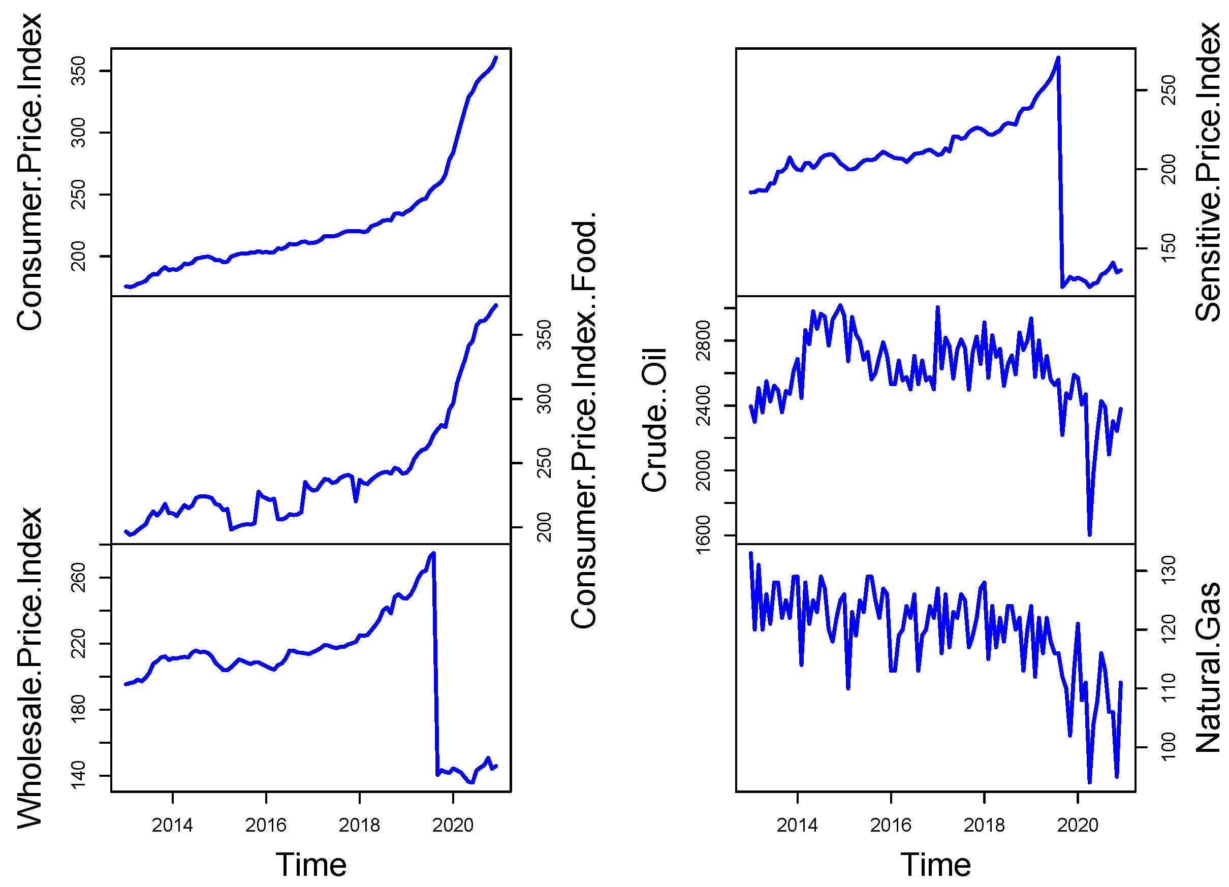
The principal macroeconomic time series dual sets for Pakistan are analyzed in this paper. The dataset includes 79 combined and de-combined variables gathered monthly between 2013 and 2020. The dataset consists of various economic sectors related to Pakistan’s economy, such as the Consumer Price Index (CPI), the Wholesale Price Index (WPI), CPI (Food), Crude Oil, SPI, Natural gas prices, the external sector, real estate, another financial and monetary sector, and the fiscal part, etc. The graphical representation of these variables can be seen in
Figure 3. For instance, CPI experienced a sudden rise near 2020, which indicates significant price increases, also known as inflation. The price of consumer goods experienced an expanding trend that abruptly increased due to an economic event during the pandemic. Throughout the graph, the costs of goods and services consistently increase until they reach their peak.
However, the WPI experienced a strong upward movement in the year 2020, which resulted in a significant price reduction. The wholesale price index displays a major downturn following 2020 that suggests market equilibrium is taking place because supply chains are disrupted and demand is unbalanced. Market changes and unpredictable eventsike global crises create economic instabilities that immediately affect prices. On the other hand, the CPI (Food) price index shows a similar upward movement to the CPI while experiencing a significant increase in 2020. A steep rise in food prices occurred, which might stem from supply chain disruptions and agricultural disturbances generated by international events. The rising food prices demonstrates how fundamental items respond strongly to external economic factors in the global market. In contrast, minimal fluctuations exist within the crude oil plot, presenting an elevated point during 2020, followed by an immediate decline. Oil market prices underwent significant changes because of reduced global needs due to COVID-19, OPEC actions, and political conflict between nations. Oil market sensitivity causes abrupt fluctuations in crude oil prices resulting from external disturbances and supply–demand mismatch.
The sensitive price index shows sudden price rises in 2020, and other measurement tools are similar to its behavior. The quick price increases monitored critical goods and services during the worldwide crisis because these products showed higher sensitivity to inflationary forces. The index stabilizes following this surge, suggesting either price recovery or standardization of these prices. Meanwhile, natural gas prices show regular price shifts, which reached a prominentow point during 2020. The downward trend in gas prices appears because of pandemic-related demand decline, changes in energy consumption, and disrupted supply networks. Natural gas prices react in a volatile manner that matches the overall economic fluctuations observed throughout various businesses. Thus, the State Bank of Pakistan has assessed all this valuable information and considered all these 79 models to model and forecast one month ahead of inflation in Pakistan. Before an empirical study, all variables are converted to make them stationary. For every non-negative time series, theogarithmic transformation is often applied [
14]. To guarantee the stationarity of the variables, we used the Augmented Dickey-Fuller (ADF) test. The findings revealed that some of the variables were not stationary at their initialevel, as shown by
p-values above 0.05. To attain stationarity, we used first differencing on these variables, and after transformation, the ADF test
p-values fell below 0.05, indicating that stationarity was attained. These conversions are necessary because non-stationary data can result in poor model performance and unreliable estimates. By rectifying stationarity, we made sure that the relationship between the variables was properly captured in the following analysis.
Due to the figure’s size restriction, we cannot display the correlation matrix to assess the multicollinearity between the explanatory variables before modeling. Nonetheless, the correlation matrix displayed a substantial pairwiseink in the set of variables. Additionally, as previously mentioned, the dataset in question is a time series, even though this is rather evident. Since time series data are known to exhibit autocorrelation, autocorrelation problems are moreikely to arise in these datasets.
Figure 4 shows the monthly inflation series plotted against time. Two halves of the dataset have been divided to increase the accuracy of the out-of-sample forecast. The data for the study spans January 2013 to February 2019. And from March 2019 to December 2020 with inflation series estimation to evaluate the models’ multi-step forward post-sample prediction accuracy.
The choice to divide the data into periods before and after 2019 is based on the substantial changes in inflation patterns caused by the COVID-19 epidemic.
Figure 3 demonstrates a significant change in inflationary tendencies following 2019, which can be attributed to the severe economic disruptions induced by the epidemic. Segmentation is essential to ensure the robustness and accuracy of our study since it enables us to consider the unique economic conditions and inflationary patterns that define these two periods.
First, to determine the best model for each time series, this work calculated two accuracy metrics: the mean absolute error (MAE) and the root mean squared error (RMSE). The results of these accuracy measures are presented in
Table 1 and
Table 2.
Table 1 summarizes the accuracy mean metrics for the considered univariate methods, including AR, ARMA, NPAR, and NNA.
Table 1 shows that the AR model produced the highest forecast accuracy mean errors, outperforming all other competitors. The RMSE and the MAE values for the AR model are 0.0192 and 0.0150, respectively. The ARMA model is the second-best model, with an RMSE of 0.0192 and an MAE of 0.0151. However,
Table 2 shows the forecasting experiments conducted using several multivariate forecasting methodologies for inflation’s primary macroeconomic variable of interest. Theoss functions, or RMSE and MAE, are used to gauge forecast accuracy. Compared to alternative methods, the RMSE and MAEinked with the PLS-based factor model (shown by PLS (FM)) areower. Stated otherwise, it may be concluded that PLS (FM) outperforms its competing alternatives in the sample forecast. PLS has a better predictive capacity than its rivals when multicollinearity and autocorrelation are present. On the other hand, Autometrics generates a decent forecast, but it falls short of what PLS (FM) offers. Thus, based on the findings of
Table 1 and
Table 2, the PLS (FM) model shows superior forecasting compared to univariate and other considered multivariate models.
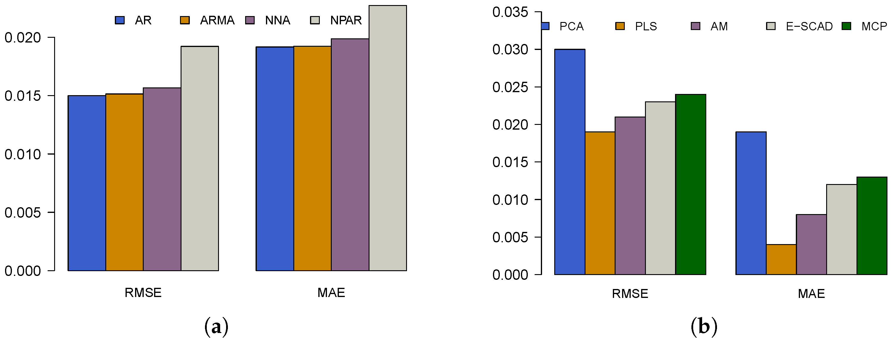
Visualization is another powerful tool for communicating the idea of the greatest technique among a group of techniques, in addition to numbers. Hence, a graphical representation of the RMSE and MAE values for all considered univariate and multivariate forecasting models is plotted in
Figure 5. In
Figure 5a, the bar plot compares accuracy measures for univariate models, including AR, ARMA, NNA, and NNAR. Theeft side of the plot represents RMSE, while the right side shows MAE. The RMSE values appear relatively similar across models, with minor variations. However, in the MAE comparison, the NPR model exhibits a noticeably higher value, suggesting that it has theeast accurate forecasts among the univariate models. The AR and ARMA models seem to haveower error values, implying better performance in this context. On the other hand, in
Figure 5b, the bar plot extends the comparison to multivariate models, including PCA, PLS, AM, E-SCAD, and MCP. The RMSE values vary significantly, with the PCA model exhibiting the highest RMSE, indicating theeast accurate predictions. Conversely, E-SCAD and MCP models display relativelyower RMSE values, suggesting superior performance. The MAE values further confirm this trend, where E-SCAD and MCP again showower error values, while PCA and AM have higher errors, indicatingess accurate predictions. Therefore, again based on graphical assessment (
Figure 5), the PLS (FM) model shows superior forecasting compared to univariate and other considered multivariate models.
This empirical analysis used accuracy mean errorsike RMSE and MAE to determine how well univariate and multivariate forecasting models performed. Then, this work conducted an equal forecasting test (the DM test) on each forecasting model pair to determine which model produced superior performance indicators (RMSE and MAE) results. The DM test results are in
Table 3 for univariate models and
Table 4 for multivariate models. In the DM test, the null hypothesis is that the row and column forecasting models have the same forecasting ability. In contrast, according to the alternative hypothesis, the column forecasting model is more accurate than the row forecasting model. Aower
p-value indicates a notable difference in the forecasting capabilities of two models, while a higher
p-value suggests that the models yield similar results.
Table 3 displays the
p-values for the univariate models (AR, ARMA, NNA, and NPAR). The diagonal entries are zero since a model is compared to itself. The NPAR model shows
p-values of 0.00 when compared to all other models, signifying that it differs significantly from all others, ikely demonstrating the poorest performance. Meanwhile, AR, ARMA, and NNA show relatively high
p-values when compared to one another (for example, AR vs. ARMA = 0.78, AR vs. NNA = 0.91), indicating that their forecasting performances are statistically comparable. This illustrates that the AR, ARMA, and NNA models do not exhibit significant variations in forecasting accuracy, whereas NPAR is notably different. On the other side,
Table 4 expands this analysis to include multivariate models, such as PCA (FM), PLS (FM), Autometrics, E-SCAD, and MCP. The results showcase greater variability among these models. For example, PCA (FM) records veryow
p-values in comparison to PLS (FM) (0.14), Autometrics (0.04), E-SCAD (0.03), and MCP (0.10), indicating that PCA differs significantly from these models. Conversely, PLS (FM) shows high
p-values against Autometrics (0.54), E-SCAD (0.62), and MCP (0.74), suggesting that these models exhibit similar forecasting effectiveness. Notably, the MCP model has significantlyow
p-values against E-SCAD (0.16), Autometrics (0.16), and PCA (0.10), highlighting some significant performance differences. In summary,
Table 3 and
Table 4 underscore important distinctions in model performance. For univariate models, NPAR is noticeably different from the others, while AR, ARMA, and NNA reflect comparable accuracy. PCA (FM) displays the most pronounced differences among multivariate models, whereas PLS (FM), Autometrics, and E-SCAD demonstrate relatively similar performanceevels. The results from the DM test offer valuable insights for selecting models that possess significantly better forecasting accuracy.
In addition to the above tabulated analysis, the DM test results (
p-values) have been plotted in
Figure 6.
Figure 6 displaysevel plots that illustrate the outcomes of the DM test concerning
p-values across various models. These tests are typically employed to assess the accuracy of forecasts between rival predictive models. In
Figure 6a, the heatmap depicts
p-values for univariate models. The x-axis and y-axis represent an array of univariate models, such as AR, ARMA, NNA, and NNR. The color gradient demonstrates the
p-values, where blue shades indicateower
p-values (reflecting significant differences in forecasting accuracy), and yellow or beige shades signify higher
p-values (indicatingess significant differences or comparable performance among models). Darker blue areas imply that specific models significantly surpass others in forecasting ability. Conversely,
Figure 6b broadens this investigation to multivariate models, which include PCA, PLS, AM, E-SCAD, and MCP. The heatmap again portrays the
p-values for model comparisons, utilizing a similar color scheme. Green and yellow areas suggest elevated
p-values, pointing towards closer performance between models, while blue zones indicateower
p-values, suggesting significant variances. The differences in color intensity imply that some models achieve considerably better performance than others while some display similar forecasting capabilities. Therefore, these figures offer a visual depiction of the results from model comparisons, aiding in identifying statistically significant variances in predictive performance. The darker blue areas emphasize where models exhibit the most disparity, while theighter yellow and green regions reflect similar forecasting effectiveness.
The difference in the models’ accuracy is not substantial, but in the forecastingiterature, even minor gains in forecasting performance are considered substantial contributions. Furthermore, it is important to note that PCA is an unsupervised model, while the other models being compared are supervised. This distinction in approach could be the reason for PCA’s underperformance in relation to the others, as it fails to use the target variable duringearning, in contrast to the supervised models, which are geared to optimize towards forecasting accuracy.
Multi-step-ahead inflation is a helpful tool for policymakers in any country in the modern world. It enables companies to analyze and readjust their various production schedules, improveogistics, and allocate resources effectively, aiding in operational planning. Various econometric tools, time series analysis, and other economic models help businesses to forecast easily. Multi-step-ahead forecasts help determine a business’s expected sales goals, inventoryevels, and profitability. When trends deviate from the roadmap, companies can take necessary actions to refocus and achieve their goals. Strategic decisions can be made based on what is and is not working.
4. Discussion
This section discusses the forecasting results in the context of model complexity and regularization, trade-offs between RMSE and MAE, practical implications for forecasting, and model selection issues.
Model Complexity and Regularization: The variations in RMSE and MAE between models capture the trade-offs between model complexity and regularization. The relatively straightforward structure of PLS (FM)—concentrating onatent components—allows it to strike a balance between the need for flexibility and the capacity to generalize well to new data. Conversely, models such as E-SCAD and MCP, which impose regularization, seem too strict for the current problem, resulting in underfitting and increased error values. Regularization can make the model more interpretable and decrease variance, but, as in this case, it can also negatively affect the model’s capacity to fit the data well when the true structure of the data is more intricate.
Trade-offs Between RMSE and MAE: The RMSE and MAE metrics give two complementary perspectives on model performance. RMSE puts more weight onarger errors because of its squaring of differences, whereas MAE gives a simpler average error metric. PLS (FM) models excel on both metrics, indicating that they not only reducearge outliers (RMSE) but also make stable and consistent predictions (MAE). On the other hand, MCP and E-SCAD have quitearge error values on both measures, suggesting that their rigid structures are preventing them from both minimizing big errors and repeatedly predicting correctly.
Practical Implications to Forecasting: In an actual forecasting context, PLS (FM) would be the ideal model with itsow RMSE and MAE, particularly in tasks with high-dimensional data and intricate variable interrelationships. PCA (FM), though optimal iness complicated datasets, would potentially perform worse under more complex scenarios; hence, ess desirable when complicated patterns need to be represented. The moderate accuracy of Autometrics indicates that it might be beneficial where model flexibility and automatic variable selection are important but may require additional tuning for some datasets.
Model Selection Issues: The trade-offs between these models emphasize the need to select a model depending on the particular forecasting task, data available, and interpretability required. Although PLS (FM) performs well in this instance, future research needs to consider the model’s scalability and its sensitivity to varying data structures. In addition, cross-validation or further testing on other datasets may yield more information regarding the robustness and generalizability of these models.
One of the major benefits of our results is that, within the Big Data context, PLS (FM) tends to be overlooked in favor of computationallyess intensive approaches. However, our findings contradict the general belief that PLS (FM) is not as effective forarge data applications, proving that it can outperform other models in multi-step-ahead forecasting even with the size of the dataset. Although techniques such as random forests or neural networks are generally favored for high-dimensional data because of their scalability, PLS (FM) has proved to be outstanding even witharge datasets. This pinpoints that PLS is able to capture intricate relationships in the data without compromising accuracy. The feature matrix (FM) methodology employed by PLS enables it to manage high-dimensionality well by concentrating on the most important parts of the data and enhancing predictive precision. In contrast to other models, e.g., PCA (FM) and Autometrics, that performed poorly witharge datasets, PLS (FM) continued to perform well, demonstrating that it can handle the demands of Big Data without overfitting or underfitting. PLS (FM) also offers a good trade-off between computational simplicity and forecasting precision, which is an important plus in practical applications. It also facilitates higher interpretability, making it possible for users to grasp the interconnection between economic variables and the target variable. Transparency is important for decision making because it offers actionable insights. Our research proves that PLS (FM) is not only scalable for Big Data but also an efficient and dependable forecasting tool that can surpass more advanced models with a highevel of interpretability. Our research further brings toight that even in recent inflation forecasting research, PLS (FM) has not been given the due attention it deserves, despite its evident benefits [
60,
61]. Most recent inflation forecasting research prefers new machineearning techniques over theikely potential of PLS (FM). Our findings show that PLS (FM) is not only scalable to Big Data but also a sound and efficient forecasting model that can outperform sophisticated models while still being highly interpretable.
To summarize and infer the findings, this research has important implications for improving the accuracy of inflation forecasting. By showing that multivariate models outperform univariate benchmarks, this study offers policymakers more accurate forecasting instruments that take into account a wider range of economic indicators. This can enable central banks to forecast inflation trends better and make proactive monetary policy changes. Secondly, the application of factor models from the study to deal with high-dimensional data enhances the capture of meaningful economic signals while eliminating noise and increasing forecast accuracy. The advancements support inflation targeting with reduced uncertainty in policy choice. The study also points to how Big Data-based forecasting methods can provide early warning indicators for inflation pressures, allowing timely actions to ensure economic stability.


 ,
, 


