Abstract
Maintaining stable prices is one of the goals of monetary policy makers. Since its formation, inflation has been a key issue and priority for every Pakistani government; it is a fundamental macroeconomic variable that plays a significant role in a nation’s economic progress and development. This research investigates the predictive capabilities of different univariate and multivariate models. The study considers autoregressive models, autoregressive neural networks, autoregressive moving average models, and other nonparametric autoregressive models within the univariate category. In contrast, the multivariate models include factor models that utilize Minimax Concave Penalty, Elastic-Smoothly Clipped Absolute Deviation, Principal Component Analysis, and Partial Least Squares. We conducted an empirical analysis using a well-established macroeconomic dataset from Pakistan. This dataset covers the period from January 2013 to December 2020 and consists of 79 variables recorded at that frequency. To evaluate the forecasting accuracy of the models for multiple steps ahead in the post-sample period, an analysis was performed using data extracted from January 2013 to February 2019 for model estimation and then another set from March 2019 to December 2020. The predictability of the univariate models following the sample period is compared with that of the multivariate models using statistical accuracy measurements, specifically root mean square error and mean absolute error. Additionally, the Diebold–Mariano test has been employed to evaluate the accuracy of the average errors statistically. The results indicated that the factor approach based on Partial Least Squares delivers significantly more effective outcomes than its competing methods.
Keywords:
fat big data; inflation forecasting; univariate and multivariate time series forecasting models; multi-step ahead forecasting; financial time series analysis; decision making MSC:
68T07; 68T09; 03H10; 37N40; 62P20; 91G15; 91G30
1. Introduction
Inflation forecasting plays a crucial role in making wise financial decisions. Nominal phrases are often used in debt, employment, tenancy, and sales contracts. For this reason, politicians, corporations, and families need to be able to foresee inflation. Furthermore, inflation projections are a critical instrument that central banks use to direct their monetary policy actions, shape inflation expectations, and advance economic stability in general. This approach helps the central bank while enabling people and companies to make better financial decisions [1,2,3,4,5].
In the past, numerous researchers projected the inflation rate through various forecasting models. For example, the study discussed in [6] analyzed how machineearning (ML) techniques enhanced inflation predictions in Brazil. By examining a comprehensive dataset and utilizing 50 distinct forecasting methods, the research showed that ML techniques often outperformed traditional econometric models the regarding mean-squared error. Furthermore, the findings emphasized the existence of nonlinearities in inflation dynamics, indicating that these methods were beneficial for macroeconomic forecasts in Brazil. Likewise, the research outlined in [7] investigated the influence of investor attention on comprehending and predicting inflation, using methods such as Granger causality tests, vector autoregression models, inear models, and various statistical indicators. The results suggested that investor attention was a Granger cause of inflation and negatively impacted it. Models that included investor attention demonstrated superior forecasting performance compared to standard benchmark models. Moreover, the paper indicated that investor attention influenced inflation through its effect on inflation expectations, underscoring its importance within macroeconomic studies.
Conversely, the research described in [8] ooked into machineearning in conjunction with traditional forecasting techniques for predicting inflation in developing countries. It evaluated whether machineearning methods were more effective than conventional approaches, noting that Random Forest and Gradient Boosting emerged as the top-performing models. The study also found that including foreign exchange reserves improved the predictive accuracy of both models. However, the work presented in [9] utilized 730,000 news articles to construct a sentiment index for US inflation forecasting via algorithmic scoring. This index outperformed a simple random walk and surpassed other benchmarks, particularly for shorter forecasting horizons, achieving a 30% reduction in root mean squared errors. In a different study [10], the authors explored the application of ML models to forecast inflation rates using a dataset consisting of 132 monthly observations from 2012 to 2022. The random forest model excelled over other models and outperformed traditional econometric methods. Nonlinear ML models, such as artificial neural networks, produced superior results due to the unpredictability and interactions among variables. The research highlighted the benefits of employing ML models for inflation forecasting and provided insights into relevant covariates that could improve policy decisions. Similarly, the investigation in [11] focused on predicting inflation in China, employing ML models that utilized an extensive array of monthly macroeconomic and financial indicators. These models exceeded the performance of standard time series and principal component regression methods, particularly during periods of substantial inflation volatility and times when the CPI and PPI diverged. Additionally, the study revealed that prices, stock market trends, and money credit were crucial factors for forecasting inflation in China. Nonetheless, the research presented in [12] forecasted UK CPI inflation metrics by analyzing monthly detailed item data spanning two decades. Ridge regression and shrinkage techniques achieved strong results for overall inflation predictions. However, the addition of macroeconomic indicators did not improve forecasting accuracy. Non-parametric machineearning techniques yielded poor forecast results, and their ability to adjust to varying signals might have resulted in increased variance, negatively impacting prediction quality.
The application of Big Data approaches has gained more attention due to recent breakthroughs in macroeconomic data collection. Accurate analysis may be accomplished when we efficiently extract and condense vital information from extensive and intricate datasets, simplifying the procedure to concentrate on the most pertinent elements. However, the performance varies according to the estimating technique and the data dimension. Due to redundant variables, dimensional reduction failures result in subpar output after a significant study by [13] on predicting using the diffusion index (DI). The standard method for analyzing data for predictive modeling is thought to be factor models. Ref. [14] demonstrated that factor models provide good forecasts as compared with currently available methods, such as bagging, pretest techniques, empirical Bayes, autoregressive forecasts, and Bayesian model averaging. It has been concluded that the DI is a valuable method for reducing the regression dimension. Still, increasing the performance without making many deviations to the prediction model is difficult. Factor models have been used aot recently for forecasting purposes, especially the ones mentioned [15,16,17,18,19].
Apart from the DI approach, sparse regression is another important instrument used in forecasting and dimension reduction, prevalent in statistics or econometrics [20]. The methods for sparse regression aim to preserve the essential features while driving the coefficients of the unimportant features to zero. The advantage of these instruments is their capacity to surmount the “curse of dimensionality”, which is a prevalent obstacle in time series data related to macroeconomics that spans extended periods. Moreover, forecasts produced by these statistical instruments have been essential in establishing beneficial monetary policies [21,22,23,24].
There are various examples of penalized regression referred to as shrinkage methods and it includes the Least Absolute Shrinkage and Selection Operator (Lasso) of [25], the Smoothly Clipped Absolute Deviation (SCAD) of [26], the Elastic Net (Enet) of [27], the adaptive Lasso of [28], the Adaptive Enet of [29], the Minimax Concave Penalty (MCP) of [30], and the regression with an Elastic SCAD (E-SCAD) of [31].
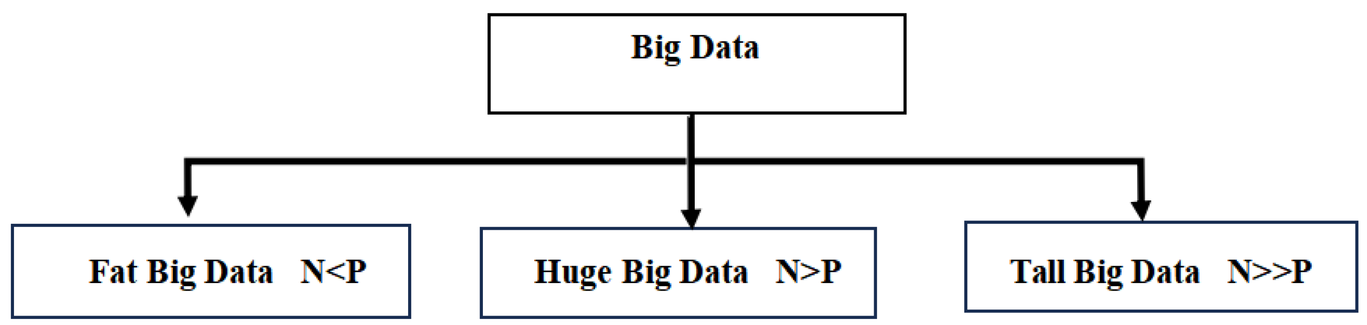
These methodologies and sparse modeling have gained popularity due to their effectiveness in managing extensive macroeconomic datasets. This approach is a compelling and noteworthy alternative to factor models, as shown by [32,33,34,35,36]. However, economic research has recently witnessed significant attention towards utilizing Big Data environments and machineearning techniques [37]. Ref. [38] suggested using penalized regression techniques for macroeconomic forecasting, but ref. [14,39,40] argued in favor of factor-based models. Additionally, Autometrics has been proposed as an effective approach by [41]. However, Big Data can be distinguished by [42], specifically in three categories. This includes Fat Big Data, Huge Big Data, and Tall Big Data, which are discussed as follows:
- The first category is Fat Big Data: In this, the number of covariates (large P) is greater than the number of observations (N).
- The second category is Tall Big Data: The number of covariates is considerablyower than the number of observations (N).
- The third category is Huge Big Data: In this category, the number of covariates (such asarge P) usually exceeds the number of observations (high N), where P and N are the number of covariates and observations, respectively.
However, the major three categories of Big data can be explained as depicted in Figure 1.
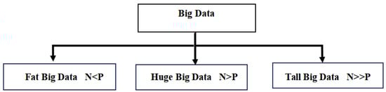
Figure 1.
Categorization of Big Data.
The earlier research focused on independent component analysis, PCA, and sparse principal component analysis to formulate factor-based models. Past studies also analyzed classical methods (Autometrics) for time series forecasting [41,42,43,44]. Other than this, there has been no study where the predictive power of the factor model based on PLS was analyzed against ML or Autometrics. Other studies have considered penalization techniquesike ridge regression, adaptiveasso, elastic net, and non-negative garrote. Other than this, no other study has used the modern version of the penalized technique for analyzing and forecasting various macroeconomic variables.
This paper fills the gaps by performing advanced methodologies for analyzing Big Data to empirically expand theiterature on macroeconomic forecasting. The recent study merely talks about Fat Big Data. Considering the dimension reduction approaches, a factor-based approach has been used to determine the effect of these aspects on various macroeconomic forecasting. For that purpose, factor-based models were constructed using PCA and PLS. Furthermore, a detailed analysis was conducted on the final form of the classical approach and modified forms of penalization techniques, namely E-SCAD and MCP. We comprehensively analyzed the analytical abilities of various factor models, classical approaches, and penalized regression. Our core focus was to conduct a comparative study of the Univariate and Multivariate models. In addition, the automatic and penalized regression tools are used against the recently developed factor models in the multivariate cases. The comparison is built using empirical application to the macroeconomic dataset. The study aims to provide an improved tool to assist practitioners and policymakers using Fat Big Data.
Another important tool in the study is inflation forecasting for directing monetary policy actions and fostering economic stability, which is the driving force behind this article. The focus area of the study was to have a better analysis regarding inflation forecast in Pakistan, a crucial element. Influencing economic results by examining univariate and multivariate models. Policymakers must comprehend the intricate interactions between economic sectors and predictive variables to control inflationary pressures properly. This study offers important insights for macroeconomic academics, practitioners, and policymakers through in-depth analysis and model comparison. The ultimate objective is to promote well-informed decision-making processes in monetary policy and economic development and to further the development of forecasting techniques.
2. Forecasting Models
The present research employs both univariate and multivariate models to predict inflation, with the former being the benchmark to test forecasting performance. However, inflation is driven by several economic variables, and thus, multivariate models are better positioned to capture the intricate relationships and enhance the precision of predictions. With the presence of Big Data, where there are more features than observations, multivariate models utilize other economic indicators to give more accurate and policy-relevant predictions.
Univariate and multivariate models are the two techniques used in this paper. This work considers the autoregressive model, autoregressive neural network, autoregressive moving average model, and non-parametric autoregressive models in univariate circumstances. On the other hand, multivariate models include factor models based on Minimax Concave Penalty, Elastic-Smoothly Clipped Absolute Deviation, Principal Component Analysis, and Partial Least Squares. The ensuing subsections contain more information on these models.
2.1. Univariate Models
This section discusses four univariate models: autoregressive, autoregressive moving average, autoregressive neural network model, and nonparametric autoregressive. The subsections that follow discuss these models in detail.
2.1.1. Autoregressive Model
In time series analysis, ainear autoregressive (AR) process is used to describe ainear combination of the n past (lags) values of a given variable, denoted as [45]. The AR process can be represented as follows:
In this equation, is a constant term (intercept), and (where ) represents the unknown parameters (slope coefficients) of the underlying AR process, respectively. The term represents the disturbance in the process.
To determine the appropriate AR process for a given time series, various criteria are used in theiterature [46]. In this case, after examining the series residuals, autocorrelation function, and partial autocorrelation function, it was found that an AR(3) process was the best fit for the data. In addition, AR (3) means that this model utilized its past threeags.
2.1.2. Nonparametric Autoregressive Model
While analyzing an additive nonparametric model, the relation between and various past values (lags) is nonlinear and is represented as an additive model:
Cubic regression splines reflect the smoothing function , which tells about the relationship between and prior (lags) values [47]. Similar to the parametric form, three delays are utilized when estimating NPAR.
2.1.3. Autoregressive Moving Average Model
The Autoregressive Moving Average (ARMA) model can be seen as one of the most important statistical tools that predicts a response variable based on its previous nags, with errors included [48]. The formula for the ARMA model can be expressed as follows:
In this mathematical equation, represents the intercept (constant), and represents the set of unknown coefficients of the AR process, represents the unknown coefficients of the MA process. Furthermore, is normally distributed. The correlograms, especially the partial and autocorrelation functions, are used to calculate the ARMA model order. In this scenario, we fitted an ARMA (3, 1) model to each series. In addition, an ARMA (3,1) model represents that this model incorporates its three previousag values, with an errorag included.
2.1.4. Neural Networks Autoregression Model
The Neural Networks Autoregression Model (NNA) is a robust computing framework that can model a broad spectrum of nonlinear issues. In contrast to other nonlinear models, NNAR can approximate a wide variety of functions with high accuracy, which is its main advantage. NNA’s concurrent processing of data information is the foundation of efficiency. The statistical modeling procedure does not give any information about the model’s geometry; rather, data attributes play an essential role in constructing node (network) models.
The multilayer perceptron, featuring hiddenayers, stands out as a widely employed artificial neural network extensively used to model time series data and make forecasts. The model consists of threeayers of fundamental processing unitsinked by interconnected circular connections. The subsequent equation elucidates how the outputs are connected () and the inputs ():
In Formula (4), (j = 0, 1, 2, …, n; k = 1, 2, …, z) and (j = 0, 1, 2, …, z) are the model unknown parameters, also calledinear weights. Here, “n” indicates theength of the input nodes, while “z” represents theength of the concealed nodes.
2.2. Multivariate Models
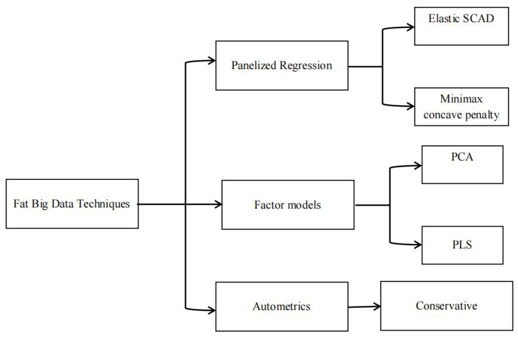
In addition to the univariate theory, we now address the theory of multivariate tools, which considers the impact of other associated (i.e., endogenous) factors on CPI in Pakistan. The CPI model for Pakistan is constructed by considering a vast number of covariates, most of which have been determined by economic theories and theiterature. Figure 2 is a graphical representation of the multivariate models used for analyzing the Fat Big Dataset.
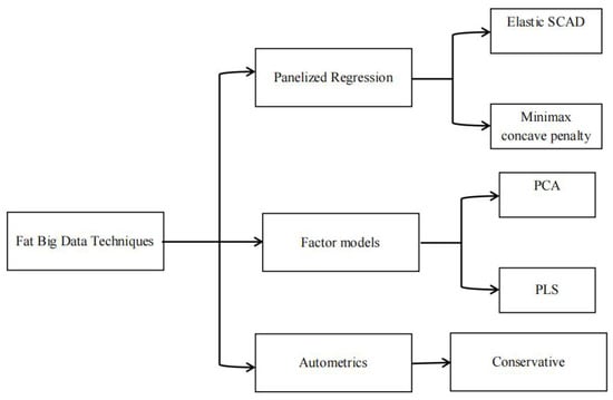
Figure 2.
Schematic representation of Fat Big Data methods [49].
2.2.1. Factor Models
Stock and Watson’s factor models, as presented in their work in [28,39,40], stand out as widely adopted techniques in macroeconomic forecasting, especially when dealing with many variables. The reason behind studying the factor model is to remove all hidden factors from the set and then analyze the data with a specific number of factors as covariates for modeling purposes. Suppose is a particular covariate.
In the above formula, the term ; , , is a vector of size ‘s’ common factors. However, is a vector of size ‘s’ factoroadings, and denotes the idiosyncratic random term.
PCA-Based Factor Model
Analysis of a factor-based model involves two steps: Initially the atent factors are extracted as principal components using all covariates by minimizing the term . In another part, the h-period out-of-sample forecast is formulated by running the principal component regression mentioned.
In the above equation, the term , the dimension of estimated coefficients is ‘s’, which can be extracted from and . A comprehensive discussion on the factors approach is provided in [13,35,40]. This mechanism is most commonly utilized in past factor analysis studies because PCs are mainly distilled by singular value decomposition [13,50,51,52].
The factor approach can provide a very good prediction if the common factors are influenced by omissions of various factors that are common [53]. Similarly, it has been [54] discussed that PCA utilizes factor structure for Z and hardly describes the response variable. Another important observation was that irrespective of the variable to be forecasted, if response variables are ignored, factor distillation will provide an accurate result.
PLS-Based Factor Model
This research considers another method that is an alternative popular approach to PCA, which is the so-called partialeast squares (PLS) regression proposed by [55]. This approach is quite good when the data is tooarge and can be an alternative to factor models designed on PCA. PLS yields various independent components by using the existing association amid covariates. PLS is effective when the number of covariates is mucharger than the various number of data points (N) and there exists multicollinearity amongst covariates.
The mathematical form of the PLS is expressed as follows:
In Equation (7), the is a vector of covariates of size observed at time is a vector of coefficients with a dimension , and is a random error. To achieve a k-period ahead of the sample forecast, we may utilize the equation given below.
2.2.2. Panelized Regression and Classical Approach
Various other methods of penalized regressionike MCP and E-SCAD, and classical method (Autometrics) are also considered in place of factor model.
Panelized Regression Methods
Various parameters of the penalized regression model are estimated by optimizing the given objective function as follows:
Minimax Concave Penalty (MCP): MCP was initially developed by [30] and corresponds to a family unit of regression with a penalty term . The chances that the MCP Penalty considers the particular model is 1. Regarding Lq-loss, the MCP estimator oracle properties provided ℵ and provide good conditions in a high dimensional setting [56]. Results are quite fruitful findings regarding variable selection, estimation, and forecasting [57].
Elastic Smoothly Clipped Absolute Deviation: Smoothly clipped absolute deviation (SCAD) was modified by adding penalty; this technique is also called elastic SCAD (E-SCAD). The E-SCAD gains a new characteristic in that the penalty function drives the inclusion or exclusion of a highly associated group having covariates [31]. Mathematically, the penalty function of E-SCAD is given as follows:
2.2.3. Classical Approach
Autometrics is a popular statistical approach designed in case of huge data [42]. Normally, the Autometrics algorithm mainly includes five steps. Initially, the model was formulatedinearly in the first step, and all covariates were included. In econometrics, such a designed model is known as the General Unrestricted Model (GUM). The next step provides us with the estimates of unknown parameters and tests them for statistical significance. The fourth step analyzed the search process and tree path search. In the next step, the model is estimated for future predictions. The end result obtained is a forecasting model using Autometrics on the GUM:
For model analysis, the moderate strategy, another named super-conservative, has been considered in a previous research paper. The results are based on a 1 percent significanceevel. Put differently, the significance of the estimated coefficients is based on a 1 percent significanceevel.
2.3. Performance Measures
Researchers have employed graphical analysis, a statistical test, and a variety of accuracy mean error metrics to analyze the performance of the univariate and multivariate time series models. To achieve this, the mean absolute error (MAE) and root mean square error (RMSE), two accuracy mean error measures for model evaluation, were applied in the current research work. These measures were obtained from the following mathematical formulas:
In the above-mentioned equations, represents the observed values, and represents the predicted values.
In addition to the above accuracy mean error measures, we utilized the Diebold and Mariano (DM) test to measure the significance of variations in predicting capabilities among models [58]. This is a commonly applied test for comparing the predictability of various models [59]. Thus, for the DM test, we considered two forecasts, and , available for the time series for . However, and are the related forecast errors. Let us define theoss allied with forecast error as , where the absoluteoss at time t is . Theoss differential between Forecast 1 and Forecast 2 for time t is thus . The null hypothesis of identical prediction accuracy for two forecasts is . Theoss differential must be stable in covariance for the DM test to be valid.
The DM test for equal prediction accuracy under these assumptions is as follows:
In this case, represents the sample meanoss differential, and is a consistent standard error estimate of .
3. Results
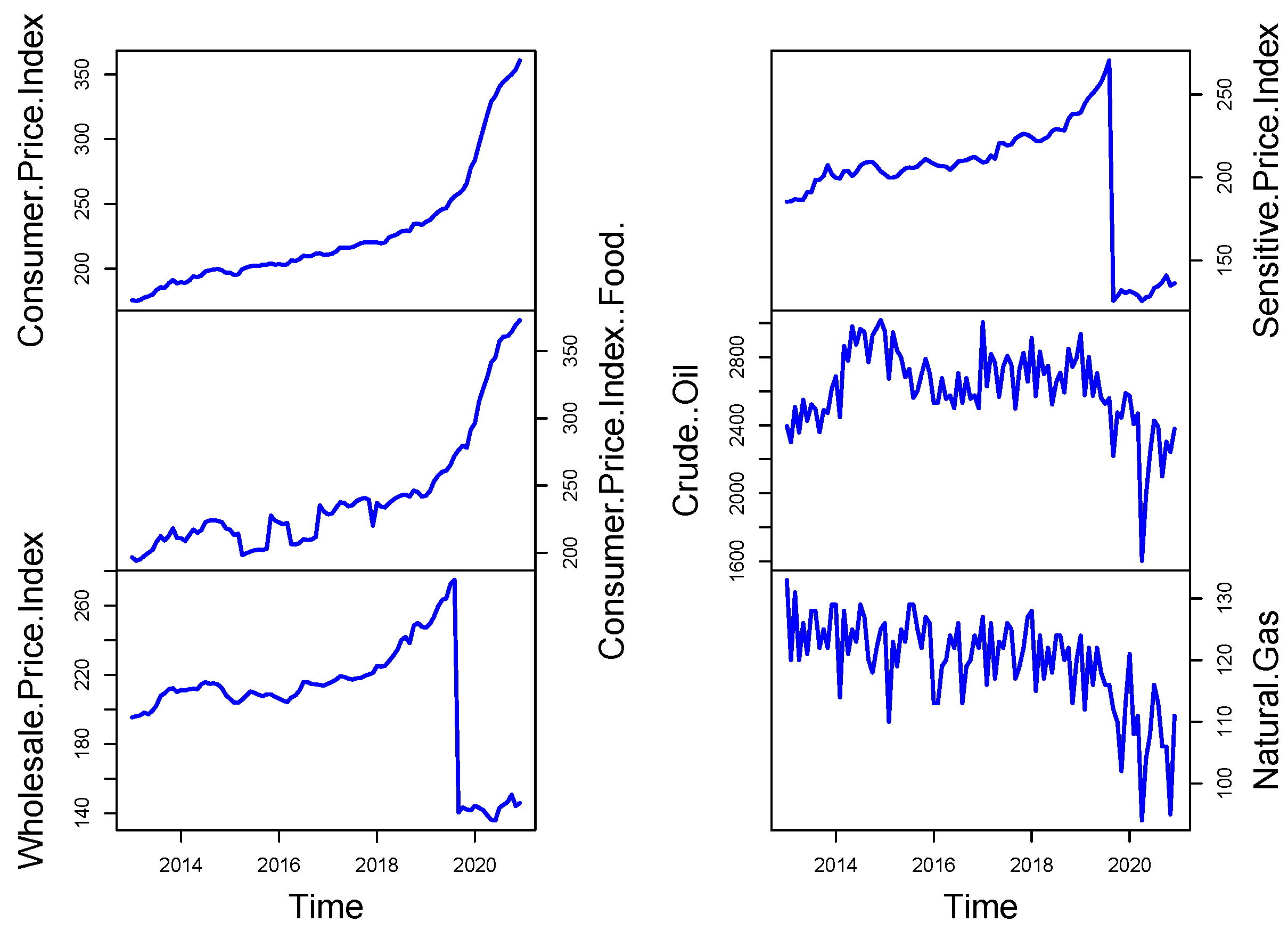
The principal macroeconomic time series dual sets for Pakistan are analyzed in this paper. The dataset includes 79 combined and de-combined variables gathered monthly between 2013 and 2020. The dataset consists of various economic sectors related to Pakistan’s economy, such as the Consumer Price Index (CPI), the Wholesale Price Index (WPI), CPI (Food), Crude Oil, SPI, Natural gas prices, the external sector, real estate, another financial and monetary sector, and the fiscal part, etc. The graphical representation of these variables can be seen in Figure 3. For instance, CPI experienced a sudden rise near 2020, which indicates significant price increases, also known as inflation. The price of consumer goods experienced an expanding trend that abruptly increased due to an economic event during the pandemic. Throughout the graph, the costs of goods and services consistently increase until they reach their peak.
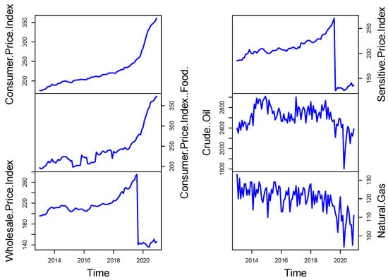
Figure 3.
The monthly time series of eight different important variables from January 2013 to December 2020.
However, the WPI experienced a strong upward movement in the year 2020, which resulted in a significant price reduction. The wholesale price index displays a major downturn following 2020 that suggests market equilibrium is taking place because supply chains are disrupted and demand is unbalanced. Market changes and unpredictable eventsike global crises create economic instabilities that immediately affect prices. On the other hand, the CPI (Food) price index shows a similar upward movement to the CPI while experiencing a significant increase in 2020. A steep rise in food prices occurred, which might stem from supply chain disruptions and agricultural disturbances generated by international events. The rising food prices demonstrates how fundamental items respond strongly to external economic factors in the global market. In contrast, minimal fluctuations exist within the crude oil plot, presenting an elevated point during 2020, followed by an immediate decline. Oil market prices underwent significant changes because of reduced global needs due to COVID-19, OPEC actions, and political conflict between nations. Oil market sensitivity causes abrupt fluctuations in crude oil prices resulting from external disturbances and supply–demand mismatch.
The sensitive price index shows sudden price rises in 2020, and other measurement tools are similar to its behavior. The quick price increases monitored critical goods and services during the worldwide crisis because these products showed higher sensitivity to inflationary forces. The index stabilizes following this surge, suggesting either price recovery or standardization of these prices. Meanwhile, natural gas prices show regular price shifts, which reached a prominentow point during 2020. The downward trend in gas prices appears because of pandemic-related demand decline, changes in energy consumption, and disrupted supply networks. Natural gas prices react in a volatile manner that matches the overall economic fluctuations observed throughout various businesses. Thus, the State Bank of Pakistan has assessed all this valuable information and considered all these 79 models to model and forecast one month ahead of inflation in Pakistan. Before an empirical study, all variables are converted to make them stationary. For every non-negative time series, theogarithmic transformation is often applied [14]. To guarantee the stationarity of the variables, we used the Augmented Dickey-Fuller (ADF) test. The findings revealed that some of the variables were not stationary at their initialevel, as shown by p-values above 0.05. To attain stationarity, we used first differencing on these variables, and after transformation, the ADF test p-values fell below 0.05, indicating that stationarity was attained. These conversions are necessary because non-stationary data can result in poor model performance and unreliable estimates. By rectifying stationarity, we made sure that the relationship between the variables was properly captured in the following analysis.
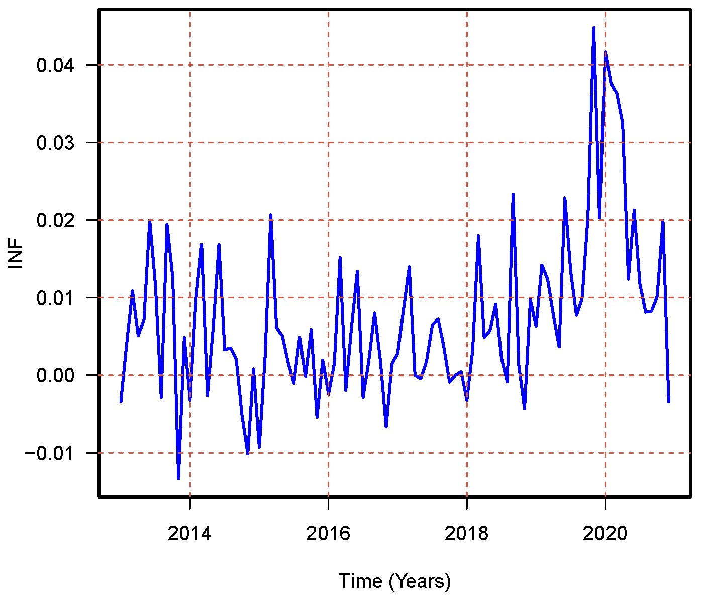
Due to the figure’s size restriction, we cannot display the correlation matrix to assess the multicollinearity between the explanatory variables before modeling. Nonetheless, the correlation matrix displayed a substantial pairwiseink in the set of variables. Additionally, as previously mentioned, the dataset in question is a time series, even though this is rather evident. Since time series data are known to exhibit autocorrelation, autocorrelation problems are moreikely to arise in these datasets. Figure 4 shows the monthly inflation series plotted against time. Two halves of the dataset have been divided to increase the accuracy of the out-of-sample forecast. The data for the study spans January 2013 to February 2019. And from March 2019 to December 2020 with inflation series estimation to evaluate the models’ multi-step forward post-sample prediction accuracy.

Figure 4.
The monthly inflation time series from January-2013 to December-2020.
The choice to divide the data into periods before and after 2019 is based on the substantial changes in inflation patterns caused by the COVID-19 epidemic. Figure 3 demonstrates a significant change in inflationary tendencies following 2019, which can be attributed to the severe economic disruptions induced by the epidemic. Segmentation is essential to ensure the robustness and accuracy of our study since it enables us to consider the unique economic conditions and inflationary patterns that define these two periods.
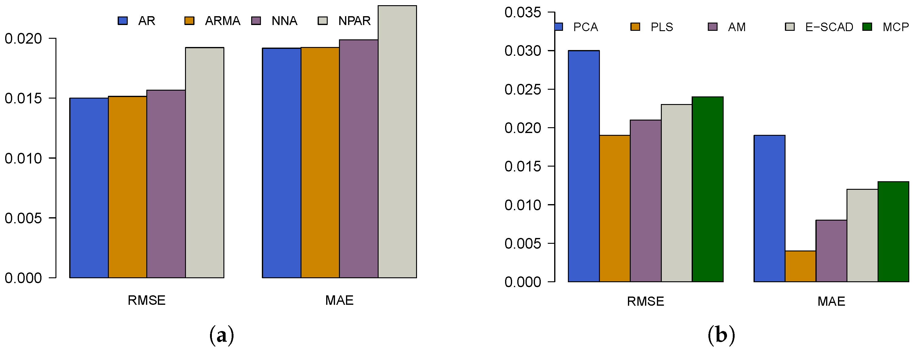
First, to determine the best model for each time series, this work calculated two accuracy metrics: the mean absolute error (MAE) and the root mean squared error (RMSE). The results of these accuracy measures are presented in Table 1 and Table 2. Table 1 summarizes the accuracy mean metrics for the considered univariate methods, including AR, ARMA, NPAR, and NNA. Table 1 shows that the AR model produced the highest forecast accuracy mean errors, outperforming all other competitors. The RMSE and the MAE values for the AR model are 0.0192 and 0.0150, respectively. The ARMA model is the second-best model, with an RMSE of 0.0192 and an MAE of 0.0151. However, Table 2 shows the forecasting experiments conducted using several multivariate forecasting methodologies for inflation’s primary macroeconomic variable of interest. Theoss functions, or RMSE and MAE, are used to gauge forecast accuracy. Compared to alternative methods, the RMSE and MAEinked with the PLS-based factor model (shown by PLS (FM)) areower. Stated otherwise, it may be concluded that PLS (FM) outperforms its competing alternatives in the sample forecast. PLS has a better predictive capacity than its rivals when multicollinearity and autocorrelation are present. On the other hand, Autometrics generates a decent forecast, but it falls short of what PLS (FM) offers. Thus, based on the findings of Table 1 and Table 2, the PLS (FM) model shows superior forecasting compared to univariate and other considered multivariate models.

Table 1.
Univariate models accuracy measures: multi-steps-ahead out-of-sample forecast for all considered univariate models.
Table 2.
Multivariate models accuracy measures: multi-steps-ahead out-of-sample forecast for all considered multivariate models.
Visualization is another powerful tool for communicating the idea of the greatest technique among a group of techniques, in addition to numbers. Hence, a graphical representation of the RMSE and MAE values for all considered univariate and multivariate forecasting models is plotted in Figure 5. In Figure 5a, the bar plot compares accuracy measures for univariate models, including AR, ARMA, NNA, and NNAR. Theeft side of the plot represents RMSE, while the right side shows MAE. The RMSE values appear relatively similar across models, with minor variations. However, in the MAE comparison, the NPR model exhibits a noticeably higher value, suggesting that it has theeast accurate forecasts among the univariate models. The AR and ARMA models seem to haveower error values, implying better performance in this context. On the other hand, in Figure 5b, the bar plot extends the comparison to multivariate models, including PCA, PLS, AM, E-SCAD, and MCP. The RMSE values vary significantly, with the PCA model exhibiting the highest RMSE, indicating theeast accurate predictions. Conversely, E-SCAD and MCP models display relativelyower RMSE values, suggesting superior performance. The MAE values further confirm this trend, where E-SCAD and MCP again showower error values, while PCA and AM have higher errors, indicatingess accurate predictions. Therefore, again based on graphical assessment (Figure 5), the PLS (FM) model shows superior forecasting compared to univariate and other considered multivariate models.
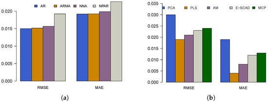
Figure 5.
Performance metrics plots: multi-step ahead accuracy measures for all considered univariate models (a) and multivariate models (b).
This empirical analysis used accuracy mean errorsike RMSE and MAE to determine how well univariate and multivariate forecasting models performed. Then, this work conducted an equal forecasting test (the DM test) on each forecasting model pair to determine which model produced superior performance indicators (RMSE and MAE) results. The DM test results are in Table 3 for univariate models and Table 4 for multivariate models. In the DM test, the null hypothesis is that the row and column forecasting models have the same forecasting ability. In contrast, according to the alternative hypothesis, the column forecasting model is more accurate than the row forecasting model. Aower p-value indicates a notable difference in the forecasting capabilities of two models, while a higher p-value suggests that the models yield similar results.
Table 3.
Diebold and Mariano test findings (p-values) for univariate models.
Table 4.
Diebold and Mariano test findings (p-values) for multivariate models.
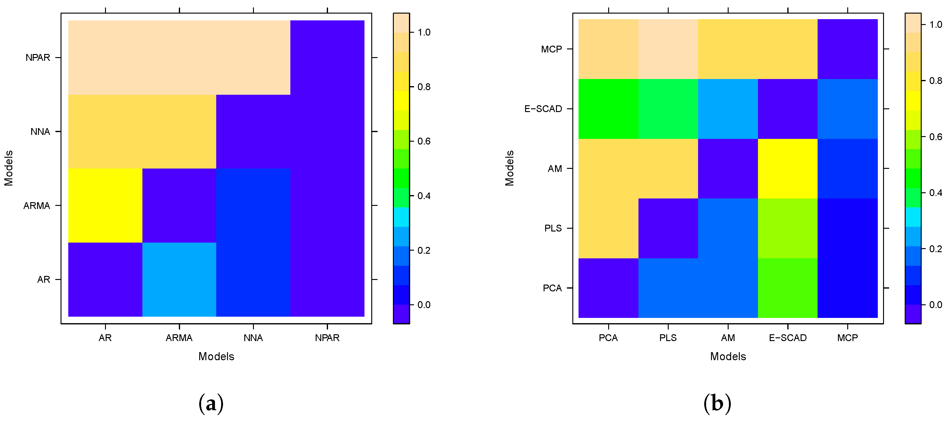
Table 3 displays the p-values for the univariate models (AR, ARMA, NNA, and NPAR). The diagonal entries are zero since a model is compared to itself. The NPAR model shows p-values of 0.00 when compared to all other models, signifying that it differs significantly from all others, ikely demonstrating the poorest performance. Meanwhile, AR, ARMA, and NNA show relatively high p-values when compared to one another (for example, AR vs. ARMA = 0.78, AR vs. NNA = 0.91), indicating that their forecasting performances are statistically comparable. This illustrates that the AR, ARMA, and NNA models do not exhibit significant variations in forecasting accuracy, whereas NPAR is notably different. On the other side, Table 4 expands this analysis to include multivariate models, such as PCA (FM), PLS (FM), Autometrics, E-SCAD, and MCP. The results showcase greater variability among these models. For example, PCA (FM) records veryow p-values in comparison to PLS (FM) (0.14), Autometrics (0.04), E-SCAD (0.03), and MCP (0.10), indicating that PCA differs significantly from these models. Conversely, PLS (FM) shows high p-values against Autometrics (0.54), E-SCAD (0.62), and MCP (0.74), suggesting that these models exhibit similar forecasting effectiveness. Notably, the MCP model has significantlyow p-values against E-SCAD (0.16), Autometrics (0.16), and PCA (0.10), highlighting some significant performance differences. In summary, Table 3 and Table 4 underscore important distinctions in model performance. For univariate models, NPAR is noticeably different from the others, while AR, ARMA, and NNA reflect comparable accuracy. PCA (FM) displays the most pronounced differences among multivariate models, whereas PLS (FM), Autometrics, and E-SCAD demonstrate relatively similar performanceevels. The results from the DM test offer valuable insights for selecting models that possess significantly better forecasting accuracy.
In addition to the above tabulated analysis, the DM test results (p-values) have been plotted in Figure 6. Figure 6 displaysevel plots that illustrate the outcomes of the DM test concerning p-values across various models. These tests are typically employed to assess the accuracy of forecasts between rival predictive models. In Figure 6a, the heatmap depicts p-values for univariate models. The x-axis and y-axis represent an array of univariate models, such as AR, ARMA, NNA, and NNR. The color gradient demonstrates the p-values, where blue shades indicateower p-values (reflecting significant differences in forecasting accuracy), and yellow or beige shades signify higher p-values (indicatingess significant differences or comparable performance among models). Darker blue areas imply that specific models significantly surpass others in forecasting ability. Conversely, Figure 6b broadens this investigation to multivariate models, which include PCA, PLS, AM, E-SCAD, and MCP. The heatmap again portrays the p-values for model comparisons, utilizing a similar color scheme. Green and yellow areas suggest elevated p-values, pointing towards closer performance between models, while blue zones indicateower p-values, suggesting significant variances. The differences in color intensity imply that some models achieve considerably better performance than others while some display similar forecasting capabilities. Therefore, these figures offer a visual depiction of the results from model comparisons, aiding in identifying statistically significant variances in predictive performance. The darker blue areas emphasize where models exhibit the most disparity, while theighter yellow and green regions reflect similar forecasting effectiveness.
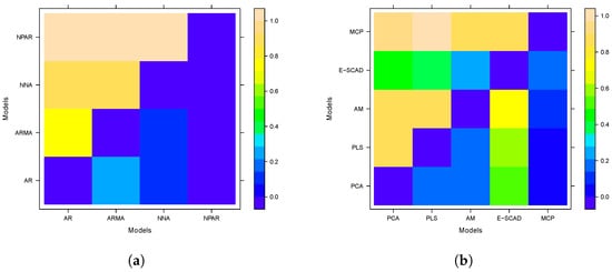
Figure 6.
Level plot: The Diebold and Mariano test findings (p-values) for all considered univariate models (a) and multivariate models (b).
The difference in the models’ accuracy is not substantial, but in the forecastingiterature, even minor gains in forecasting performance are considered substantial contributions. Furthermore, it is important to note that PCA is an unsupervised model, while the other models being compared are supervised. This distinction in approach could be the reason for PCA’s underperformance in relation to the others, as it fails to use the target variable duringearning, in contrast to the supervised models, which are geared to optimize towards forecasting accuracy.
Multi-step-ahead inflation is a helpful tool for policymakers in any country in the modern world. It enables companies to analyze and readjust their various production schedules, improveogistics, and allocate resources effectively, aiding in operational planning. Various econometric tools, time series analysis, and other economic models help businesses to forecast easily. Multi-step-ahead forecasts help determine a business’s expected sales goals, inventoryevels, and profitability. When trends deviate from the roadmap, companies can take necessary actions to refocus and achieve their goals. Strategic decisions can be made based on what is and is not working.
4. Discussion
This section discusses the forecasting results in the context of model complexity and regularization, trade-offs between RMSE and MAE, practical implications for forecasting, and model selection issues.
Model Complexity and Regularization: The variations in RMSE and MAE between models capture the trade-offs between model complexity and regularization. The relatively straightforward structure of PLS (FM)—concentrating onatent components—allows it to strike a balance between the need for flexibility and the capacity to generalize well to new data. Conversely, models such as E-SCAD and MCP, which impose regularization, seem too strict for the current problem, resulting in underfitting and increased error values. Regularization can make the model more interpretable and decrease variance, but, as in this case, it can also negatively affect the model’s capacity to fit the data well when the true structure of the data is more intricate.
Trade-offs Between RMSE and MAE: The RMSE and MAE metrics give two complementary perspectives on model performance. RMSE puts more weight onarger errors because of its squaring of differences, whereas MAE gives a simpler average error metric. PLS (FM) models excel on both metrics, indicating that they not only reducearge outliers (RMSE) but also make stable and consistent predictions (MAE). On the other hand, MCP and E-SCAD have quitearge error values on both measures, suggesting that their rigid structures are preventing them from both minimizing big errors and repeatedly predicting correctly.
Practical Implications to Forecasting: In an actual forecasting context, PLS (FM) would be the ideal model with itsow RMSE and MAE, particularly in tasks with high-dimensional data and intricate variable interrelationships. PCA (FM), though optimal iness complicated datasets, would potentially perform worse under more complex scenarios; hence, ess desirable when complicated patterns need to be represented. The moderate accuracy of Autometrics indicates that it might be beneficial where model flexibility and automatic variable selection are important but may require additional tuning for some datasets.
Model Selection Issues: The trade-offs between these models emphasize the need to select a model depending on the particular forecasting task, data available, and interpretability required. Although PLS (FM) performs well in this instance, future research needs to consider the model’s scalability and its sensitivity to varying data structures. In addition, cross-validation or further testing on other datasets may yield more information regarding the robustness and generalizability of these models.
One of the major benefits of our results is that, within the Big Data context, PLS (FM) tends to be overlooked in favor of computationallyess intensive approaches. However, our findings contradict the general belief that PLS (FM) is not as effective forarge data applications, proving that it can outperform other models in multi-step-ahead forecasting even with the size of the dataset. Although techniques such as random forests or neural networks are generally favored for high-dimensional data because of their scalability, PLS (FM) has proved to be outstanding even witharge datasets. This pinpoints that PLS is able to capture intricate relationships in the data without compromising accuracy. The feature matrix (FM) methodology employed by PLS enables it to manage high-dimensionality well by concentrating on the most important parts of the data and enhancing predictive precision. In contrast to other models, e.g., PCA (FM) and Autometrics, that performed poorly witharge datasets, PLS (FM) continued to perform well, demonstrating that it can handle the demands of Big Data without overfitting or underfitting. PLS (FM) also offers a good trade-off between computational simplicity and forecasting precision, which is an important plus in practical applications. It also facilitates higher interpretability, making it possible for users to grasp the interconnection between economic variables and the target variable. Transparency is important for decision making because it offers actionable insights. Our research proves that PLS (FM) is not only scalable for Big Data but also an efficient and dependable forecasting tool that can surpass more advanced models with a highevel of interpretability. Our research further brings toight that even in recent inflation forecasting research, PLS (FM) has not been given the due attention it deserves, despite its evident benefits [60,61]. Most recent inflation forecasting research prefers new machineearning techniques over theikely potential of PLS (FM). Our findings show that PLS (FM) is not only scalable to Big Data but also a sound and efficient forecasting model that can outperform sophisticated models while still being highly interpretable.
To summarize and infer the findings, this research has important implications for improving the accuracy of inflation forecasting. By showing that multivariate models outperform univariate benchmarks, this study offers policymakers more accurate forecasting instruments that take into account a wider range of economic indicators. This can enable central banks to forecast inflation trends better and make proactive monetary policy changes. Secondly, the application of factor models from the study to deal with high-dimensional data enhances the capture of meaningful economic signals while eliminating noise and increasing forecast accuracy. The advancements support inflation targeting with reduced uncertainty in policy choice. The study also points to how Big Data-based forecasting methods can provide early warning indicators for inflation pressures, allowing timely actions to ensure economic stability.
5. Concluding Remarks
Stabilizing prices is one of the objectives of monetary policymakers. Inflation has remained the main manifesto and concern of any Pakistani government since independence; it is one of the essential macro variables to be considered for a country’s economic development and growth. Our main aim is to know the most popular model with respect to time series forecasting, such as the factor model, that is performed against classical and shrinkage methods. The study was carried out on Pakistan’s macroeconomic data. The dataset entails 79-time series that were tracked with a monthly frequency and cover a time period starting from January 2013 to December 2020. This vast dataset has been obtained directly from our main source i.e., State Bank of Pakistan. The data considered for the study covers a time period from January 2013 to February 2019 and from March 2019 to December 2020. The study aims to estimate models’ multi-step-ahead out-of-sample predictive performance. RMSE and MAE have been employed to examine and compare the prediction accuracy of factor models in 359 in contrast to Autometrics and ML techniques in the post-sample analysis. For policy analysis, achieving an accurate inflation forecast is challenging in a data-rich environment. This study can help policymakers, who are expected to anticipate future economic developments and account for the minimum advance. The results of this study support those of [43], highlighting the conclusions’ reliability and consistency in various situations. This alignment reinforces the robustness of the identified relationships, contributing to a comprehensive understanding of the phenomenon.
From a policy point of view, the results of this paper identify a key role for multivariate models in enhancing inflation forecasting accuracy, an essential ingredient in central banks’ response in monetary policy formulation. The paper illustrates that historic univariate approaches are good benchmarks but haveimited capability to identify the nuanced relationships driving the dynamics of inflation. In addition to using various economic measures, the multivariate models offer more precise and robust forecasts, enabling policymakers to make informed choices that stabilize inflation and maintain economic stability. The findings highlight the importance of central banks embracing sophisticated forecasting methods in order to forecast inflationary developments effectively and take proactive measures accordingly. Finally, this research promotes evidence-based policymaking by providing insights into the best choice of model for inflation forecasting.
In the future, researchers can improve forecasting accuracy by employing a hybrid strategy that integrates dimension-reduction techniques with machineearning models instead of depending on individual models. This integrated approach enables more effective handling of data with aarge number of dimensions and can reveal intricate patterns, resulting in more precise and reliable forecasts. By focusing on the advantages of dimension reduction and machineearning, researchers may create models that are more accurate and capable of handling the complexities of real-world data.
Author Contributions
Conceptualization, methodology, and software, F.K. and H.I.; validation, F.K., H.I., A.A.A. and P.C.R.; formal analysis, H.I.; investigation, H.I., F.K. and P.C.R.; resources, A.A.A., J.A. and P.C.R.; data curation, H.I. and F.K.; writing—original draft preparation, F.K., H.I. and P.C.R.; writing—review and editing, F.K., H.I., A.A.A., P.C.R. and J.A.; visualization, J.A., P.C.R. and H.I.; supervision, P.C.R. and H.I.; project administration, H.I., J.A. and P.C.R.; funding acquisition, A.A.A., J.A. and P.C.R. All authors have read and agreed to the published version of the manuscript.
Funding
This research received no external funding.
Data Availability Statement
The data used in this study are available at https://www.sbp.org.pk/index.html (accessed on 20 January 2023).
Conflicts of Interest
The authors declare no conflicts of interest.
References
- Medeiros, M.C.; Vasconcelos, G.F.; Veiga, A.; Zilberman, E. Forecasting inflation in a data-rich environment: The benefits of machineearning methods. J. Bus. Econ. Stat. 2021, 39, 98–119. [Google Scholar]
- Bilgil, H. New Grey Forecasting Model with Its Application and Computer Code. AIMS Math. 2021, 6, 1497–1514. [Google Scholar] [CrossRef]
- Chen, Q.; Han, Y.; Huang, Y.; Jiang, G.J. Jump Risk Implicit in Options Market. J. Financ. Econom. 2025, 23, nbaf002. [Google Scholar] [CrossRef]
- He, Q.; Xia, P.; Hu, C.; Li, B. Public information, actual intervention and inflation expectations. Transform. Bus. Econ. 2022, 21, 644–666. [Google Scholar]
- Zhou, Z.; Zhou, X.; Qi, H.; Li, N.; Mi, C. Near miss prediction in commercial aviation through a combined model of grey neural network. Expert Syst. Appl. 2024, 255, 124690. [Google Scholar] [CrossRef]
- Araujo, G.S.; Gaglianone, W.P. Machineearning methods for inflation forecasting in Brazil: New contenders versus classical models. Latin Am. J. Cent. Bank. 2023, 4, 100087. [Google Scholar] [CrossRef]
- Zhu, P.; Zhou, Q.; Zhang, Y. Investor attention and consumer price index inflation rate: Evidence from the United States. Humanit. Soc. Sci. Commun. 2024, 11, 541. [Google Scholar]
- Mirza, N.; Rizvi, S.K.A.; Naqvi, B.; Umar, M. Inflation prediction in emerging economies: Machineearning and FX reserves integration for enhanced forecasting. Int. Rev. Financ. Anal. 2024, 94, 103238. [Google Scholar] [CrossRef]
- Eugster, P.; Uhl, M.W. Forecasting inflation using sentiment. Econ. Lett. 2024, 236, 111575. [Google Scholar] [CrossRef]
- Das, P.K.; Das, P.K. Forecasting and Analyzing Predictors of Inflation Rate: Using Machine Learning Approach. J. Quant. Econ. 2024, 22, 493–517. [Google Scholar] [CrossRef]
- Huang, N.; Qi, Y.; Xia, J. China’s inflation forecasting in a data-rich environment: Based on machineearning algorithms. Appl. Econ. 2024, 1–26. [Google Scholar] [CrossRef]
- Joseph, A.; Potjagailo, G.; Chakraborty, C.; Kapetanios, G. Forecasting UK inflation bottom up. Int. J. Forecast. 2024, 40, 1521–1538. [Google Scholar] [CrossRef]
- Stock, J.H.; Watson, M.W. Macroeconomic forecasting using diffusion indexes. J. Bus. Econ. Stat. 2002, 20, 147–162. [Google Scholar]
- Stock, J.H.; Watson, M.W. Generalized shrinkage methods for forecasting using many predictors. J. Bus. Econ. Stat. 2012, 30, 481–493. [Google Scholar]
- Bai, J.; Liao, Y. Efficient estimation of approximate factor models via penalized maximumikelihood. J. Econom. 2016, 191, 1–18. [Google Scholar]
- Fan, J.; Li, R. Statistical challenges with high dimensionality: Feature selection in knowledge discovery. arXiv 2006, arXiv:math/0602133. [Google Scholar]
- Chang, X.; Gao, H.; LI, W. Discontinuous Distribution of Test Statistics Around Significance Thresholds in Empirical Accounting Studies. J. Account. Res. 2025, 63, 165–206. [Google Scholar] [CrossRef]
- Jin, H.; Tian, S.; Hu, J.; Zhu, L.; Zhang, S. Robust ratio-typed test forocation change under strong mixing heavy-tailed time series model. Commun. Stat.—Theory Methods 2025, 1–24. [Google Scholar] [CrossRef]
- Fan, J.; Liao, Y.; Wang, W. Projected principal component analysis in factor models. Ann. Stat. 2016, 44, 219. [Google Scholar]
- Shi, Q.; Sun, Y.; Saanouni, T. On the growth of Sobolev norms for Hartree equation. J. Evol. Equ. 2025, 25, 13. [Google Scholar] [CrossRef]
- Bernanke, B.S.; Boivin, J.; Eliasz, P. Measuring the effects of monetary policy: A factor-augmented vector autoregressive (favar) approach. Q. J. Econ. 2005, 120, 387–422. [Google Scholar]
- Syed, A.A.S.; Lee, K.H. Macroeconomic forecasting for Pakistan in a data-rich environment. Appl. Econ. 2021, 53, 1077–1091. [Google Scholar] [CrossRef]
- Öztürk, Z.; Bilgil, H.; Erdinç, Ü. An optimized continuous fractional grey model for forecasting of the time dependent real world cases. Hacet. J. Math. Stat. 2022, 51, 308–326. [Google Scholar] [CrossRef]
- Liu, K.; Luo, J.; Faridi, M.Z.; Nazar, R.; Ali, S. Green shoots in uncertain times: Decoding the asymmetric nexus between monetary policy uncertainty and renewable energy. Energy Environ. 2025, 0958305X241310198. [Google Scholar] [CrossRef]
- Tibshirani, R. Regression shrinkage and selection via theasso. J. R. Stat. Soc. Ser. (Methodol.) 1996, 58, 267–288. [Google Scholar] [CrossRef]
- Fan, J.; Li, R. Variable selection via nonconcave penalizedikelihood and its oracle properties. J. Am. Stat. Assoc. 2001, 96, 1348–1360. [Google Scholar] [CrossRef]
- Zou, H.; Hastie, T. Regularization and variable selection via the elastic net. J. R. Stat. Soc. Ser. (Statistical Methodol.) 2005, 67, 301–320. [Google Scholar] [CrossRef]
- Zou, H. The adaptiveasso and its oracle properties. J. Am. Stat. Assoc. 2006, 101, 1418–1429. [Google Scholar] [CrossRef]
- Zou, H.; Zhang, H.H. On the adaptive elastic-net with a diverging number of parameters. Ann. Stat. 2009, 37, 1733. [Google Scholar] [CrossRef]
- Zhang, C.-H. Nearly unbiased variable selection under minimax concave penalty. Ann. Statist. 2010, 38, 894–942. [Google Scholar] [CrossRef]
- Zeng, L.; Xie, J. Group variable selection via scad-l2. Statistics 2014, 48, 49–66. [Google Scholar]
- Castle, J.L.; Clements, M.P.; Hendry, D.F. Forecasting by factors, by variables, by both or neither? J. Econom. 2013, 177, 305–319. [Google Scholar]
- Luciani, M. Forecasting with approximate dynamic factor models: The role of nonpervasive shocks. Int. J. Forecast. 2014, 30, 20–29. [Google Scholar]
- Iftikhar, H.; Zafar, A.; Turpo-Chaparro, J.E.; Canas Rodrigues, P.; López-Gonzales, J.L. Forecasting day-ahead Brent crude oil prices using hybrid combinations of time series models. Mathematics 2023, 11, 3548. [Google Scholar] [CrossRef]
- Kim, H.H.; Swanson, N.R. Mining big data using parsimonious factor, machineearning, variable selection and shrinkage methods. Int. J. Forecast. 2018, 34, 339–354. [Google Scholar]
- Erdinç, Ü.; Bilgil, H. Analyzing coal consumption in china: Forecasting with the ecfgm(1, 1) model and a perspective on the future. Turk. J. Forecast. 2024, 8, 45–53. [Google Scholar]
- Maehashi, K.; Shintani, M. Macroeconomic forecasting using factor models and machineearning: An application to japan. J. Jpn. Int. Econ. 2020, 58, 101104. [Google Scholar]
- Kim, H.H.; Swanson, N.R. Forecasting financial and macroeconomic variables using data reduction methods: New empirical evidence. J. Econom. 2014, 178, 352–367. [Google Scholar]
- Stock, J.H.; Watson, M.W. Forecasting inflation. J. Monet. Econ. 1999, 44, 293–335. [Google Scholar]
- Stock, J.H.; Watson, M.W. Forecasting using principal components from aarge number of predictors. J. Am. Stat. Assoc. 2002, 97, 1167–1179. [Google Scholar]
- Castle, J.L.; Doornik, J.A.; Hendry, D.F. Modelling non-stationary big data. Int. J. Forecast. 2021, 37, 1556–1575. [Google Scholar]
- Doornik, J.A.; Hendry, D.F. Statistical model selection with big data. Cogent Econ. Financ. 2015, 3, 1045216. [Google Scholar]
- Khan, F.; Urooj, A.; Khan, S.A.; Alsubie, A.; Almaspoor, Z.; Muhammadullah, S. Comparing the forecast performance of advanced statistical and machineearning techniques using huge big data: Evidence from Monte Carlo experiments. Complexity 2021, 2021, 6117513. [Google Scholar]
- Luo, J.; Zhuo, W.; Xu, B. A Deep Neural Network-Based Assistive Decision Method for Financial Risk Prediction in Carbon Trading Market. J. Circuits, Syst. Comput. 2023, 33, 2450153. [Google Scholar] [CrossRef]
- Iftikhar, H.; Khan, M.; Turpo-Chaparro, J.E.; Rodrigues, P.C.; López-Gonzales, J.L. Forecasting stock prices using a novel filtering-combination technique: Application to the Pakistan stock exchange. AIMS Math. 2024, 9, 3264–3288. [Google Scholar]
- Gonzales, S.M.; Iftikhar, H.; López-Gonzales, J.L. Analysis and forecasting of electricity prices using an improved time series ensemble approach: An application to the Peruvian electricity market. AIMS Math. 2024, 9, 21952–21971. [Google Scholar]
- Iftikhar, H.; Khan, F.; Torres Armas, E.A.; Rodrigues, P.C.; López-Gonzales, J.L. A novel hybrid framework for forecasting stock indices based on the nonlinear time series models. Comput. Stat. 2025, 1–24. [Google Scholar] [CrossRef]
- Qureshi, M.; Iftikhar, H.; Rodrigues, P.C.; Rehman, M.Z.; Salar, S.A. Statistical modeling to improve time series forecasting using machineearning, time series, and hybrid models: A case study of bitcoin price forecasting. Mathematics 2024, 12, 3666. [Google Scholar]
- Khan, F.; Albalawi, O. Analysis of Fat Big Data Using Factor Models and Penalization Techniques: A Monte Carlo Simulation and Application. Axioms 2024, 13, 418. [Google Scholar] [CrossRef]
- Bai, J.; Ng, S. Confidence intervals for diffusion index forecasts and inference for factor-augmented regressions. Econometrica 2006, 74, 1133–1150. [Google Scholar]
- Bai, J.; Ng, S. Determining the number of factors in approximate factor models. Econometrica 2002, 70, 191–221. [Google Scholar] [CrossRef]
- Xu, A.; Wang, W.; Zhu, Y. Does smart city pilot policy reduce CO2 emissions from industrial firms? Insights from China. J. Innov. Knowl. 2023, 8, 100367. [Google Scholar] [CrossRef]
- Boivin, J.; Ng, S. Are more data always better for factor analysis? J. Econom. 2006, 132, 169–194. [Google Scholar] [CrossRef]
- Tu, Y.; Lee, T.-H. Forecasting using supervised factor models. J. Manag. Sci. Eng. 2019, 4, 12–27. [Google Scholar] [CrossRef]
- Wold, H. Soft Modeling: The Basic Design and Some Extensions. In Systems Under Indirect Observation: Part II; Jöreskog, K.G., Wold, H., Eds.; Amsterdam: North-Holland, The Netherlands, 1982; pp. 1–54. [Google Scholar]
- Wang, Y.; Fan, Q.; Zhu, L. Variable selection and estimation using a continuous approximation to the 0 penalty. Ann. Inst. Stat. Math. 2018, 70, 191–214. [Google Scholar] [CrossRef]
- Li, N.; Yang, H. Nonnegative estimation and variable selection under minimax concave penalty for sparse high-dimensionalinear regression models. Stat. Pap. 2021, 62, 661–680. [Google Scholar] [CrossRef]
- Diebold, F.X. Comparing predictive accuracy, twenty yearsater: A personal perspective on the use and abuse of Diebold-Mariano tests. J. Bus. Econ. Stat. 2015, 33, 1. [Google Scholar] [CrossRef]
- Carbo-Bustinza, N.; Iftikhar, H.; Belmonte, M.; Cabello-Torres, R.J.; De La Cruz, A.R.H.; Lopez-Gonzales, J.L. Short-term forecasting of ozone concentration in metropolitan Lima using hybrid combinations of time series models. Appl. Sci. 2023, 13, 10514. [Google Scholar] [CrossRef]
- Naghi, A.A.; O’Neill, E.; Danielova Zaharieva, M. The benefits of forecasting inflation with machineearning: New evidence. J. Appl. Econom. 2024, 39, 1321–1331. [Google Scholar] [CrossRef]
- Liu, Y.; Pan, R.; Xu, R. Mending the Crystal Ball: Enhanced Inflation Forecasts with Machine Learning; IMF Working Paper No. 2024/206; International Monetary Fund: Washington, DC, USA, 2024. [Google Scholar]
Disclaimer/Publisher’s Note: The statements, opinions and data contained in all publications are solely those of the individual author(s) and contributor(s) and not of MDPI and/or the editor(s). MDPI and/or the editor(s) disclaim responsibility for any injury to people or property resulting from any ideas, methods, instructions or products referred to in the content. |
© 2025 by the authors. Licensee MDPI, Basel, Switzerland. This article is an open access article distributed under the terms and conditions of the Creative Commons Attribution (CC BY) license (https://creativecommons.org/licenses/by/4.0/).