Enhancing Border Learning for Better Image Denoising

Abstract

Deep neural networks for image denoising typically follow an encoder–decoder model, with convolutional (Conv) layers as essential components. Conv layers apply zero padding at the borders of input data to maintain consistent output dimensions. However, zero padding introduces ring-like artifacts at the borders of output images, referred to as border effects, which negatively impact the network’s ability to learn effective features. In traditional methods, these border effects, associated with convolutional/deconvolutional operations, have been mitigated using patch-based techniques. Inspired by this observation, patch-wise denoising algorithms were explored to derive a CNN architecture that avoids border effects. Specifically, we extend the patch-wise autoencoder to learn image mappings through patch extraction and patch-averaging operations, demonstrating that the patch-wise autoencoder is equivalent to a specific convolutional neural network (CNN) architecture, resulting in a novel residual block. This new residual block includes a mask that enhances the CNN’s ability to learn border features and eliminates border artifacts, referred to as the Border-Enhanced Residual Block (BERBlock). By stacking BERBlocks, we constructed a U-Net denoiser (BERUNet). Experiments on public datasets demonstrate that the proposed BERUNet achieves outstanding performance. The proposed network architecture is built on rigorous mathematical derivations, making its working mechanism highly interpretable. The code and all pretrained models are publicly available.

1. Introduction

For the denoising task, the objective is to estimate a clean image of the same size from a noisy input. Encoder–decoder models have been effectively utilized in deep learning to achieve this goal, including fully convolutional networks (FCNs) [1,2,3], U-Net [4,5,6], non-local neural networks (NLNNs) [7,8,9,10], and Transformers [11,12,13]. These architectures serve as fundamental components in more complex deep neural networks (DNNs) such as unfolding networks [14,15,16], generative adversarial networks (GANs) [17,18,19], and diffusion models [20,21,22]. Despite the continuous emergence of increasingly complex DNNs, convolution (Conv) layers remain fundamental, as they can be stacked to form encoders and decoders in FCNs and U-Net, enhance local feature representations in NLNNs and Transformers, and facilitate data transformations across different processing stages in more sophisticated DNNs.

The mathematical formula for convolution is given by $\mathit{y}=\mathit{k}⊛\mathit{x}$, where $\mathit{x}$ represents the input image, $\mathit{k}$ is the convolution kernel, and $\mathit{y}$ denotes the convolution result. Since the essence of image convolution is the weighted sum of pixels within a sliding window, it can be represented in an equivalent matrix form $y_i=\mathit{K}{\mathit{P}}_i\mathit{x}$, where ${\mathit{P}}_i$ refers to the i-th convolution window extracted from the image $\mathit{x}$, $\mathit{K}$ represents the convolution kernel in matrix form, and $y_i$ is the output for that window. However, as shown in the formula, the weighted sum of the elements within each window of $\mathit{x}$ results in a single element $y_i$, which causes the size of $\mathit{y}$ to be smaller than that of $\mathit{x}$. A common practice is to pad the borders of the data with zeros before convolution.

Zero padding in convolution is crucial for deep convolutional neural networks (CNN). On one hand, zero padding ensures that the data size remains unchanged during the forward pass of the network, facilitating the design of deeper network architectures and significantly enhancing the network’s ability to represent denoising features [23,24]. On the other hand, convolutions with zero padding are mathematically equivalent to deconvolutions (TConv) with data cropping [25], which explains why convolutions can function as decoders (this will be discussed in Section 3.4).

However, zero padding has been observed to introduce border effects in CNNs [26]. As shown on the left side of Figure 1, zero padding adds irrelevant information to the convolution window ${\mathit{P}}_i\mathit{x}$ at the image borders and requires specific convolution kernels [27]. CNNs tend to learn convolutional weights that represent image features, which do not handle the border features introduced by zero padding very well [28]. This leads to circular artifacts at the image borders in the outputs of consecutive Conv layers. Figure 1 illustrates this issue, showing the feature map output from the third scale, fourth residual block of DRUNet [4] when denoising the ‘house’ image.

In fact, this border effect has also been observed in traditional methods based on convolution/deconvolution [29]. Meanwhile, traditional patch-based methods have been validated in practice to avoid this border effect [30]. This is because patches are extracted from the image in an overlapping manner and then averaged to reconstruct the image. Each patch is encoded and decoded independently, and data padding does not affect the normal image texture. This property has been utilized in inpainting tasks [31]. The latest algorithm-unfolded DNNs, such as DKSVD [32] and LIDIA [33], have explicitly incorporated patch extraction and patch-averaging layers into their architectures, but the handcrafted patch denoisers do not fully leverage the advantages of patch-based DNNs.

The autoencoder model more suitable for patch denoising in deep learning caught our attention. With the help of patch extraction and patch averaging, the patch-wise autoencoder can be directly learned from the image, forming a feedforward neural network block for image mapping. In the model derivation, the proposed block has a similar structure to the basic residual block in CNNs, but it enhances the learning of border features, thus it is named the Border-Enhanced Residual Block (BERBlock). We further construct a U-Net-based denoiser using BERBlock as an instance for discussion, named BERUNet.

In this study, quantitative metrics including parameter size, giga floating-point operations per second (GFLOPs), peak GPU memory, and average inference time are used to evaluate the computational overhead of BERBlock and BERUNet. To verify the theoretical properties of BERBlock, we introduce paired t-tests, feature maps, average accuracy maps, and relative accuracy maps. The final denoising performance of BERUNet is rigorously assessed using quantitative peak signal-to-noise ratio (PSNR), structural similarity index map (SSIM), and qualitative visual comparisons. The calculation method for feature maps can be found in [34], while the methods for average accuracy maps and relative accuracy maps are detailed in Section 4.2.2 and Section 4.2.3, respectively. Other metrics are implemented using publicly available computing packages for Python (version 3.8), including fvcore (0.1.5), NumPy (1.22.3), OpenCV (4.6.0), and PyTorch (1.12.0). Extensive ablation studies and multi-candidate tests are conducted to compare various models, ensuring a comprehensive evaluation of the proposed method against competing approaches.

Specifically, this paper includes the following contributions:

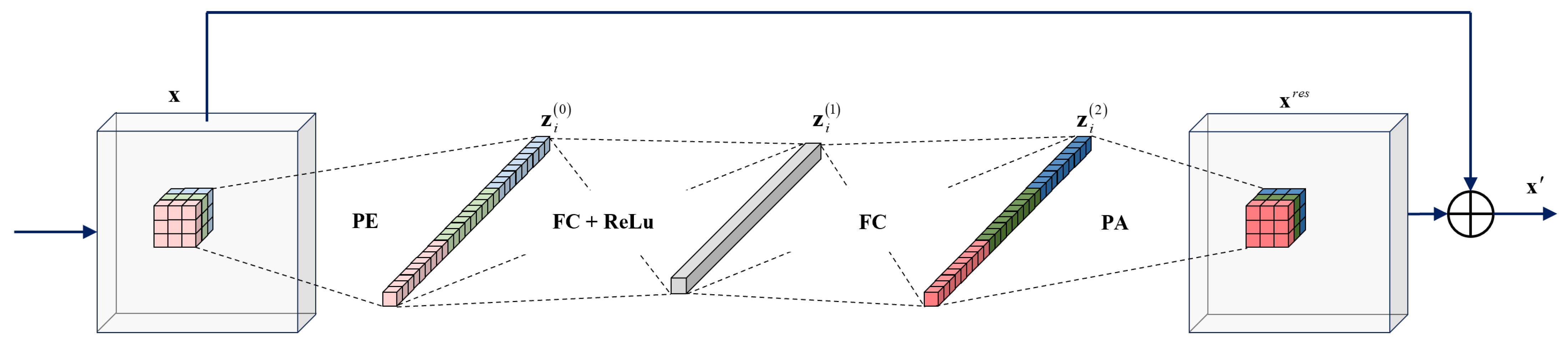
• The patch-wise autoencoder model is extended into a novel residual block to learn image mappings. This block is designed with a specific CNN configuration for efficient computation, demonstrating superior performance in peak GPU memory usage and average inference time.
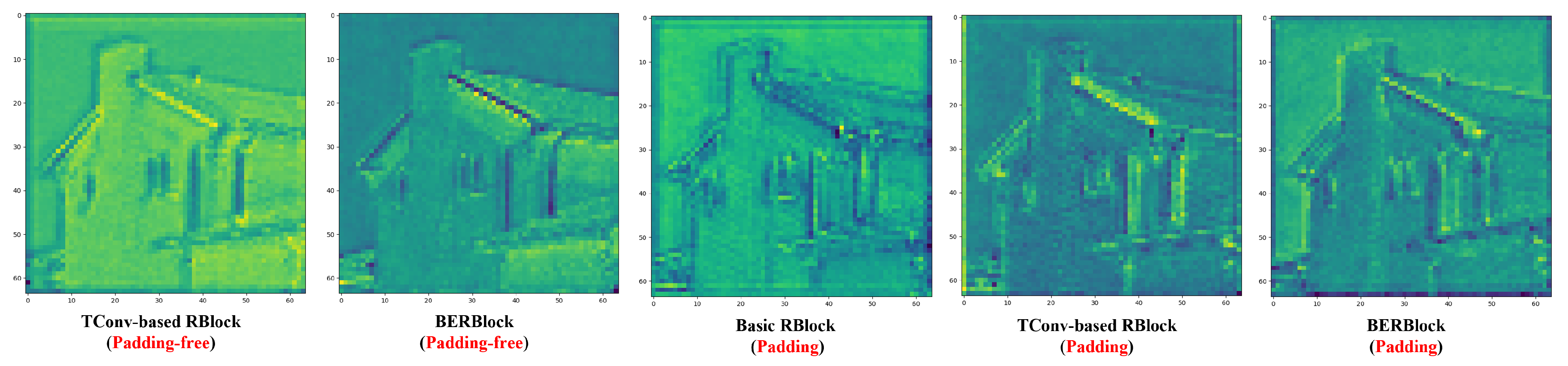
• Compared to the basic residual block, the proposed residual block enhances the learning of border features, effectively eliminating high-frequency artifacts in feature maps propagated within the CNN. This improves the accuracy of high-frequency texture restoration in denoised results.
• Extensive comparisons with 19 state-of-the-art DNN-based methods on benchmark datasets Set12, BSD68, Kodak24, McMaster, Urban100, and SIDD across different noise removal tasks demonstrate that the proposed residual block enables U-Net-based denoisers to achieve outstanding performance in terms of PSNR, SSIM, visual quality, and average inference time.

2. Related Work

To design the Border-Enhanced Residual Block (BERBlock) and develop the denoising method (BERUNet) based on it, this chapter provides the foundational theory and related work essential for our approach.

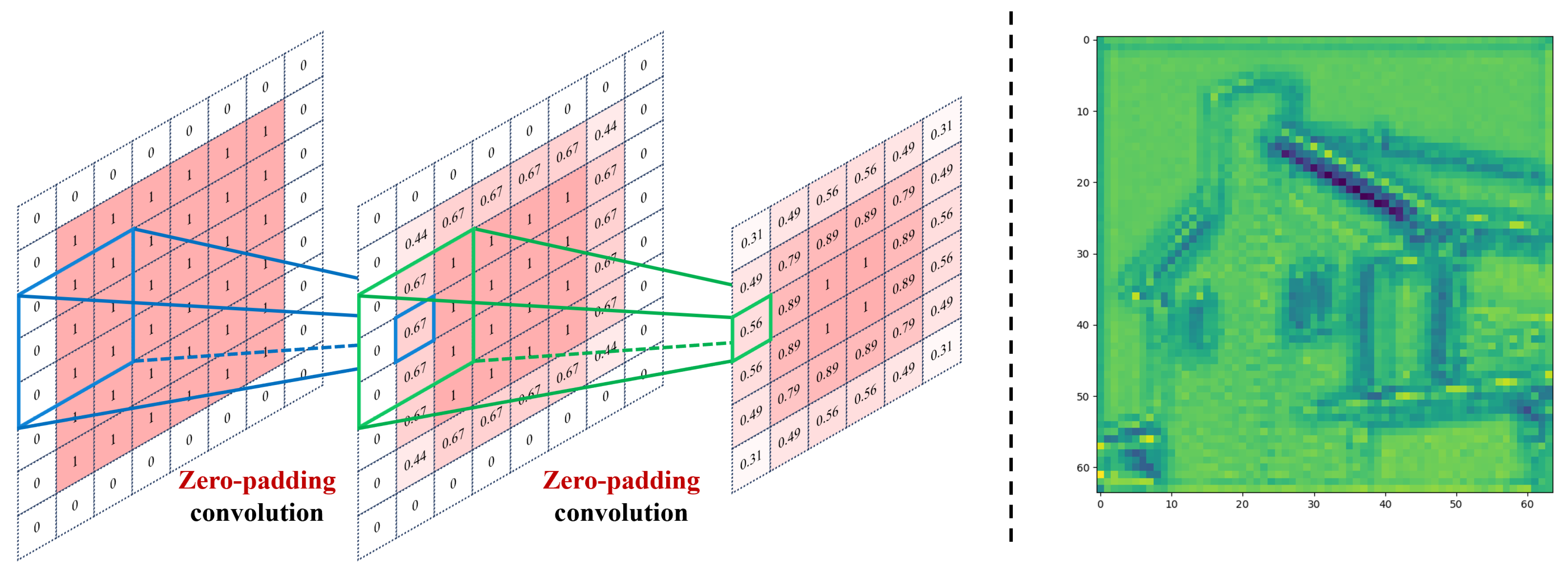
2.1. Solution to the Border Effect in CNNs

Zero-padding convolution is widely used in DNN-based denoisers, stemming from AlexNet [35] and VGG [36], where zero padding was employed to maintain feature map dimensions during the forward pass. However, in recent years, zero padding has been observed to introduce bias in image borders, reducing the generalizability and robustness of the model [27,28]. To address this issue, cyclic, replicate, reflection, and dynamic padding have been proposed as alternatives to zero padding [34,37,38] or special convolution methods have been designed to attempt to learn accurate parameters from padded data [39,40,41].

These methods all add complex operations to the CNN model, which not only reduces the computational efficiency of the CNN but also undermines the algorithmic interpretability of CNNs in solving application tasks. Therefore, they cannot replace zero-padding convolution.

2.2. Patch-Wise Denoiser Learned from Whole Images

In traditional denoising methods, patch-based algorithms do not exhibit border effects and achieve better denoising performance than convolution-based methods, such as the well-known BM3D [42], EPLL [30], KSVD [43], WMMN [44], and NCSR [45]. These patch-based algorithms have also inspired improvements in DNNs. On one hand, traditional patch-based algorithms have been expanded into end-to-end DNNs, leading to models like NLRN [7], CSCNet [46], DCT2Net [47], DKSVD [32], and LIDIA [33]. On the other hand, by defining patch data within DNNs, architectures such as Graph Convolutional Networks (GCN) [48] and Transformers [49] have been successfully applied to image denoising. Unlike traditional methods, patch-based DNNs learn patch-wise denoisers from the whole image in an end-to-end manner, resulting in a significant performance boost.

In these patch-based DNNs, DKSVD and LIDIA explicitly define patch extraction and patch-averaging layers instead of using Conv layers, which helps avoid the border effects. However, DKSVD and LIDIA use traditional algorithms as patch denoisers, which limits their denoising performance.

2.3. Autoencoders for Image Patch Denoising

The concept of an autoencoder was initially introduced by Rumelhart [50] as a neural network designed to extract data features, consisting of an encoder and a decoder. It typically comprises an input layer, one or more hidden layers, and an output layer, making it a typical multilayer perceptron (MLP) [51]. In 2008, Vincent et al. [52] proposed the Denoising Autoencoder (DAE), aiming to learn robust representations to reconstruct clean data from noisy input. In 2012, Burger et al. [53] demonstrated that MLP could function as a patch-wise denoiser, and in the same year, Xie et al. [54] introduced SSDA, the first DAE trained to denoise image patches. With the continued development of autoencoder theory [55,56], various autoencoder-based denoisers such as AMC-SSDA [57], LLNet [58], GSAE [59], and SNA [60] have been successively proposed.

These autoencoder-based denoisers are trained on small-sized images or patches, and cannot match the performance of end-to-end networks in large-sized image tasks. However, if the autoencoder is used as the patch-wise denoiser in KSVD, it can directly handle large-sized image tasks as part of an end-to-end network. Additionally, the matrix operations on patches are equivalent to a new CNN block, which can alleviate the border effects of consecutive convolutions.

3. Methodology

In this chapter, we introduce a novel convolution-based residual block, referred to as BERBlock, which is derived from a patch-wise autoencoder. A comparative analysis is presented between the conventional basic residual block and the proposed BERBlock. Additionally, we describe the integration of BERBlock into a U-Net-based network for image denoising, which we name BERUNet.

3.1. Learn Patch-Wise Mapping by Residual Autoencoder

Compared to noisy image patches, the features of clean image patches exhibit greater sparsity. As a result, sparse learning has been proposed for image patch denoising, typically involving two steps: extracting sparse features by encoder and reconstructing clean image patches by decoder. Among the sparse feature learning algorithms, autoencoders have garnered attention due to their use of the backpropagation algorithm to train neural networks with specific architectures.

An autoencoder is a self-supervised neural network designed to learn latent representations from the training data ${\mathit{z}}^{gt}$ or its corrupted form, with the objective of reconstructing the ${\mathit{z}}^{gt}$. In its simplest form, given a d-dimensional input vector ${\mathit{z}}^{in}$, a fully connected mapping extracts its $d^{\prime }$-dimensional hidden representation ${\mathit{z}}^{hid}=\mathcal{R}\left({\mathit{W}}^{\left(1\right)}{\mathit{z}}^{in}+{\mathit{b}}^{\left(1\right)}\right)$, where ${\mathit{W}}^{\left(1\right)}\in {\mathbb{R}}^{d^{\prime }\times d}$, ${\mathit{b}}^{\left(1\right)}\in {\mathbb{R}}^{d^{\prime }}$, and $\mathcal{R}$ is a nonlinear activation function, typically ReLU, referred to as the encoder. Another fully connected mapping is used to reconstruct the output from the hidden layer ${\mathit{z}}^{out}={\mathit{W}}^{\left(2\right)}{\mathit{z}}^{hid}+{\mathit{b}}^{\left(2\right)}$, where ${\mathit{z}}^{out}$ is consistent with the dimension of ${\mathit{z}}^{in}$, ${\mathit{W}}^{\left(2\right)}\in {\mathbb{R}}^{d\times d^{\prime }}$, and ${\mathit{b}}^{\left(2\right)}\in {\mathbb{R}}^d$, known as the decoder. Therefore, an autoencoder maps the input to the output via

$$\begin{array}{c}\hfill {\mathit{z}}^{out}={\mathcal{F}}_{\mathit{W},\mathit{b}}\left({\mathit{z}}^{in}\right)={\mathit{W}}^{\left(2\right)}\mathcal{R}\left({\mathit{W}}^{\left(1\right)}{\mathit{z}}^{in}+{\mathit{b}}^{\left(1\right)}\right)+{\mathit{b}}^{\left(2\right)}.\end{array}$$

(1)

Inspired by residual networks, Tran et al. [61] proposed the residual autoencoder (RAE) and trained the autoencoder within a DNN. In the RAE, the output ${\mathit{z}}^{out}$ of the autoencoder is expected to approximate $\Delta \mathit{z}=\mathit{z}-{\mathit{z}}^{in}$, resulting in the following mathematical mapping:

$$\begin{array}{c}\hfill \begin{array}{ccc}{\mathit{z}}^{\prime }={\mathcal{H}}_{\mathit{W},\mathit{b}}\left({\mathit{z}}^{in}\right)={\mathcal{F}}_{\mathit{W},\mathit{b}}\left({\mathit{z}}^{in}\right)+{\mathit{z}}^{in}& s.t.& {\mathit{z}}^{\prime }\to {\mathit{z}}^{gt}\end{array}.\end{array}$$

(2)

In this paper, Equation (2) is used to learn the mapping from noisy patches to clean patches, serving as the patch-wise denoiser for the DNN.

3.2. From Patch-Wise Autoencoder to Image-Wise Mapping

In existing research, the parameters of the autoencoder model are learned from a patch dataset, which limits the model’s ability to capture the correlation between adjacent patches, since each patch is treated independently. In contrast, although convolution is essentially a weighted sum of pixels within a window, CNNs directly learn convolutional weights from the image, enabling them to better capture the correlation between adjacent windows.

We note that Scetbon et al. [32] proposed DKSVD, which explicitly defines a patch extraction layer and a patch-averaging layer within the DNN, successfully undertaking end-to-end learning of the Iterative Shrinkage Thresholding Algorithm (ISTA) [62] for filtering patches from the image. Inspired by DKSVD, in this paper, we use the patch extraction layer and patch-averaging layers to learn the autoencoder-based mapping for patches.

The patch extraction process can be written in the following matrix form:

$$\begin{array}{c}\hfill {\mathit{z}}_i=\mathcal{P}\left(\mathit{x}\right)={\mathit{P}}_i\mathit{x},\end{array}$$

(3)

where $\mathit{x}$ represents a tensor that represents the image or feature map, ${\mathit{z}}_i$ denotes the i-th patch, and ${\mathit{P}}_i$ represents the operation matrix for extracting ${\mathit{z}}_i$ from the tensor $\mathit{x}$. In contrast, reconstructing the patches back into the image can be written as

$$\begin{array}{c}\hfill \mathit{x}={\mathcal{P}}^{-1}\left({\mathit{z}}_i\right)={\left({\sum }_i{\mathit{P}}_i^{\mathrm{T}}{\mathit{P}}_i\right)}^{-1}\left({\sum }_i{\mathit{P}}_i^{\mathrm{T}}{\mathit{z}}_i\right).\end{array}$$

(4)

Zoran et al. [30] found that when patches are extracted with overlap using Equation (3), the overlapping regions between adjacent patches introduce correlations that can enhance the denoising performance of the patch-wise denoiser. In this context, in Equation (4), the operation ${\sum }_i{\mathit{P}}_i^{\mathrm{T}}{\mathit{z}}_i$ accumulates the patches, while ${\sum }_i{\mathit{P}}_i^{\mathrm{T}}{\mathit{P}}_i$ normalizes the accumulated pixels by the accumulated weights. Therefore, in this work, following the definition in [32], we refer to Equation (4) as patch averaging.

By incorporating the patch-wise mapping model described in Equation (2) into Equations (3) and (4), we can establish the following mapping from the input image $\mathit{x}$ to the output image ${\mathit{x}}^{\prime }$:

$$\begin{array}{cc}\hfill {\mathit{x}}^{\prime }=& \hfill {\mathcal{P}}^{-1}\left({\mathcal{H}}_{\mathit{W},\mathit{b}}\left(\mathcal{P}\left(\mathit{x}\right)\right)\right)={\mathcal{P}}^{-1}\left({\mathcal{F}}_{\mathit{W},\mathit{b}}\left(\mathcal{P}\left(\mathit{x}\right)\right)+\mathcal{P}\left(\mathit{x}\right)\right)={\mathcal{P}}^{-1}\left({\mathcal{F}}_{\mathit{W},\mathit{b}}\left(\mathcal{P}\left(\mathit{x}\right)\right)\right)+\mathit{x}.\hfill \end{array}$$

(5)

Equation (5) represents residual learning for the image-wise mapping, and this formulation can be realized by feedforward neural networks. To construct the feedforward network, Equation (5) is first decomposed into the following subfunctions:

$$\begin{array}{cc}\hfill {\mathit{z}}_i^{\left(0\right)}=& \hfill {\mathit{P}}_i\mathit{x},\hfill \end{array}$$

(6a)

$$\begin{array}{cc}\hfill {\mathit{z}}_i^{\left(1\right)}=& \hfill \mathcal{R}\left({\mathit{w}}^{\left(1\right)}{\mathit{z}}_i^{\left(0\right)}+{\mathit{b}}^{\left(1\right)}\right),\hfill \end{array}$$

(6b)

$$\begin{array}{cc}\hfill {\mathit{z}}_i^{\left(2\right)}=& \hfill {\mathit{W}}^{\left(2\right)}{\mathit{z}}_i^{\left(1\right)}+{\mathit{b}}^{\left(2\right)},\hfill \end{array}$$

(6c)

$$\begin{array}{cc}\hfill {\mathit{x}}^{res}=& \hfill {\left({\sum }_i{\mathit{P}}_i^{\mathrm{T}}{\mathit{P}}_i\right)}^{-1}\left({\sum }_i{\mathit{P}}_i^{\mathrm{T}}{\mathit{z}}_i^{\left(2\right)}\right),\hfill \end{array}$$

(6d)

$$\begin{array}{cc}\hfill {\mathit{x}}^{\prime }=& \hfill \mathit{x}+{\mathit{x}}^{res}.\hfill \end{array}$$

(6e)

where Equation (6a) represents a patch extraction (PE) layer in the network, Equation (6b) represents a fully connected (FC) layer with a ReLU activation function, Equation (6c) represents another FC layer, Equation (6d) represents a patch-averaging (PA) layer, and Equation (6e) represents a residual layer. These layers are stacked sequentially to form a feedforward network, as shown in Figure 2.

Figure 2 illustrates the explicit structure of Equation (5) in the neural network. The first FC layer, with the ReLU activation function, serves as the encoder for patch-wise mapping, where ${\mathit{W}}^{\left(1\right)}$ and ${\mathit{b}}^{\left(1\right)}$ are its learnable parameters. The second FC layer acts as the decoder for the patch-wise mapping, and ${\mathit{W}}^{\left(2\right)}$ and ${\mathit{b}}^{\left(2\right)}$ are its learnable parameters. With the help of the sub-network in Figure 2, the parameters of the patch-wise mapping are learned end-to-end from the image.

3.3. Accelerate Patch-Wise Autoencoder by Conv and TConv Layers

Although the PE layer, FC layer, and PA layer shown in Figure 2 are matrix operations that can be parallelized on the GPU and theoretically have high computational efficiency, in practical engineering, we observed that the patch matrices consume a large amount of GPU memory, and considerable time is spent on memory allocation and data read/write operations (see explicit BERBlock in

Table 1. Computational cost of different residual blocks for $64\times 256\times 256$ input data.

Block Structure	Explicit BERBlock		Implicit BERBlock		Basic RBlock		TConv-Based RBlock
Padding/Cropping	✓	×	✓	×	✓	×	✓	×
Parameter size (K)	73.856		73.856		73.856		73.856
GFLOPs	4.832	4.757	4.832	4.757	4.832	-	4.832	4.757
Peak GPU memory (MB)	501.286	494.715	84.782	84.713	64.282	-	64.282	64.281
Average inference time (ms)	3.495	3.364	0.840	0.850	0.664	-	0.667	0.666

). Additionally, efficient computation libraries such as cuDNN cannot be fully leveraged. To improve the computational efficiency of Equation (5) during both training and inference, we transform the patch-wise matrix operations into convolution and deconvolution operations, which are more efficiently implemented using Conv and TConv layers.

First, we combine the formulas of the PE layer and the first FC layer, and the resulting formula is as follows:

$$\begin{array}{c}\hfill {\mathit{z}}_i^{\left(1\right)}=\mathcal{R}\left({\mathit{W}}^{\left(1\right)}{\mathit{P}}_i\mathit{x}+{\mathit{b}}^{\left(1\right)}\right).\end{array}$$

(7)

Equation (7) includes patch-wise feature extraction ${\mathit{W}}^{\left(1\right)}{\mathit{P}}_i\mathit{x}+{\mathit{b}}^{\left(1\right)}$ and the activation function $\mathcal{R}$. ${\mathit{W}}^{\left(1\right)}{\mathit{P}}_i\mathit{x}$ also represents a weighted sum of the window pixels, which is mathematically equivalent to the matrix form of convolution. According to [63], we can replace the parallel computation of the PE and the first FC layer with a faster Conv layer in CNNs.

Similarly, by combining the computation formulas of the second FC layer and the PA layer, the resulting equation can be expressed as follows:

$$\begin{array}{c}\hfill {\mathit{x}}^{\prime }={\left({\sum }_i{\mathit{P}}_i^{\mathrm{T}}{\mathit{P}}_i\right)}^{-1}\left[{\sum }_i{\mathit{P}}_i^{\mathrm{T}}\left({\mathit{W}}^{\left(2\right)}{\mathit{z}}_i^{\left(1\right)}+{\mathit{b}}^{\left(2\right)}\right)\right],\end{array}$$

(8)

where ${\mathit{b}}^{\left(2\right)}$ represents the bias applied to the reconstructed patches. Assuming that the same bias is applied to the patch vectors from each channel, while the biases between channels differ, the biases for all channels are concatenated into ${\mathit{b}}^{\prime }$. In this case, Equation (8) is equivalent to the following form:

$$\begin{array}{c}\hfill {\mathit{x}}^{\prime }={\left({\sum }_i{\mathit{P}}_i^{\mathrm{T}}{\mathit{P}}_i\right)}^{-1}\left({\sum }_i{\mathit{P}}_i^{\mathrm{T}}{\mathit{W}}^{\left(2\right)}{\mathit{z}}_i^{\left(1\right)}\right)+{\mathit{b}}^{\prime },\end{array}$$

(9)

The right side of Equation (9) can be split into three terms: ${\left({\sum }_i{\mathit{P}}_i^{\mathrm{T}}{\mathit{P}}_i\right)}^{-1}$, ${\sum }_i{\mathit{P}}_i^{\mathrm{T}}{\mathit{W}}^{\left(2\right)}{\mathit{z}}_i^{\left(1\right)}$ and a learnable bias ${\mathit{b}}^{\prime }$. ${\sum }_i{\mathit{P}}_i^{\mathrm{T}}{\mathit{W}}^{\left(2\right)}{\mathit{z}}_i^{\left(1\right)}$ is used to recover local pixels from the features and reassemble them into the image based on their positions, which is consistent with the definition of a TConv layer without bias in CNNs [64]. Meanwhile, ${\left({\sum }_i{\mathit{P}}_i^{\mathrm{T}}{\mathit{P}}_i\right)}^{-1}$ generates a mask for each pixel, indicating the weights removed from each pixel in the image. This suggests that the second FC layer and the PA layer can be accelerated using TConv layers, simple mask multiplication, and bias addition.

Therefore, the explicit structure shown in Figure 2 is equivalent to a faster implicit structure shown in Figure 3. The implicit structure consists of a Conv layer with ReLU, a TConv layer, a mask layer, a bias layer, and a residual layer. On one hand, this avoids the large GPU memory consumption caused by patch matrices; on the other hand, it enables faster computation using existing tools.

The mask layer in Figure 3 is crucial for our network. From a mathematical perspective, it is derived from the PA layer and computed using ${\left({\sum }_i{\mathit{P}}_i^{\mathrm{T}}{\mathit{P}}_i\right)}^{-1}$, ensuring that the weights of the Conv and TConv layers can be interpreted as the weights for patch-wise autoencoder. From a data perspective, the values at the borders of the mask are higher, which compensates for the attenuated border information during the forward pass and emphasizes the border gradients during the backward pass. This improves the residual block’s ability to learn border features. Therefore, the subnetworks in Figure 2 and Figure 3 are named Border-Enhanced Residual Blocks, abbreviated as BERBlock. Figure 2 illustrates the explicit BERBlock, while Figure 3 illustrates the implicit BERBlock.

Table 1 presents the computational cost of the implicit BERBlock, where the number of hidden layer channels in the residual modules is set to 64, matching the input data dimensionality. The average inference time is measured by executing each residual block 1000 times on a Titan V GPU and computing the mean. It can be observed that, compared to the unoptimized explicit BERBlock, although the number of parameters and computational cost (GFLOPs) per block remain unchanged, GPU memory consumption is reduced by $83.09\%$, and computational speed is improved by $3.16\times$. The computational cost of the implicit BERBlock is close to that of the efficient basic residual blocks (basic RBlock and TConv-based RBlock, which will be introduced in the next section). For convenience, BERBlock will hereafter refer to the implicit BERBlock in Figure 3.

It is worth noting that directly using ${\left({\sum }_i{\mathit{P}}_i^{\mathrm{T}}{\mathit{P}}_i\right)}^{-1}$ as the mask will scale the gradients during backpropagation, causing the DNN stacked with BERBlocks to fail in training. Therefore, in practice, we compute the mask using $\alpha {\left({\sum }_i{\mathit{P}}_i^{\mathrm{T}}{\mathit{P}}_i\right)}^{-1}$, where $\alpha$ is a scaling factor and $\alpha$ is set to the average of ${\sum }_i{\mathit{P}}_i^{\mathrm{T}}{\mathit{P}}_i$. In the derivation of BERBlock shown in Equation (5), scaling the mask by a factor of $\alpha$ is equivalent to proportionally shrinking the network parameters $\mathit{W}$ and $\mathit{b}$.

3.4. The Relationship and Difference with the Basic Residual Block

The Conv and TConv layers make BERBlock a typical CNN block, enabling us to leverage techniques that have been extensively validated in CNNs to enhance the performance of BERBlock. Below, we first discuss the relationship between BERBlock and the basic residual block (RBlock).

Returning to the basic RBlock proposed by He et al. [65], shown in Figure 4a, it consists of two Conv layers with ReLU activation and a shortcut connection. Each Conv layer uses a $3\times 3$ kernel. To ensure that the data dimensions remain unchanged before and after convolution, zero padding with a width of 1 is applied to the borders of the input data in all Conv layers.

The basic RBlock and BERBlock may seem to differ significantly. Therefore, we begin by analyzing the basic RBlock. The matrix form of the convolution window mentioned in the introduction, $y_i=\mathit{K}{\mathit{P}}_i\mathit{x}$, can be expanded as follows:

$$\begin{array}{c}\hfill y_i={\sum }_j{k}_j{x}_{i,j}=k_1{x}_{i,1}+k_2{x}_{i,2}+...,\end{array}$$

(10)

Here, $x_{i,j}$ represents the j-th element in the window ${\mathit{P}}_i$ and $k_j$ denotes the j-th element of the convolution kernel $\mathit{K}$. As described in [64], Equation (10) can also be expressed as the summation of overlapping elements in adjacent windows from the deconvolution output, indicating that convolution and deconvolution are mathematically equivalent. Therefore, deconvolution is referred to as transposed convolution (TConv) in CNNs.

The equivalence of convolution and deconvolution based on Equation (10) does not take image borders into account. Shi et al. [25] discovered that applying zero padding to the input of a Conv layer is effectively equivalent to cropping the output of a TConv layer by the same width. Based on this, we replace the second Conv layer in the RBlock with an equivalent TConv layer, resulting in the residual block shown in Figure 4b. This equivalent TConv layer has a $3\times 3$ kernel size and performs cropping with a width of 1 on the output data borders. Therefore, the basic RBlock can be interpreted as an encoder–decoder model based on deconvolutional networks, as proposed in [66].

Therefore, using the TConv-based RBlock as a bridge provides a better perspective on the relationship and differences between BERBlock and the basic RBlock. This reveals the following two notable differences between them:

• The mask layer in BERBlock enhances the learning of border features in the image;
• The basic RBlock uses data padding/cropping to preserve the size of the hidden layers.

In theory, data padding and cropping are unnecessary for the TConv-based RBlock and the proposed BERBlock, and using valid convolutions can avoid the border bias described in [26,34]. However, Al-Saggaf et al. [67] experimentally verified that padding data in Conv layers benefits CNNs by ensuring that each layer of the network passes sufficient image information, improving the training accuracy of the network parameters. Inspired by this, we believe that applying zero padding to the input data and cropping the output data can similarly enhance the performance of BERBlock, with the distinction that the mask layer in BERBlock helps mitigate the border effect. Related experiments will be presented in Section 4.1.3 and Section 4.2.

3.5. Network Architectures for Image Denoising

As discussed in the previous section, BERBlock can be viewed as an alternative to the basic residual block, used in state-of-the-art DNNs. To provide instances for discussion, we describe a U-Net-based model with BERBlock for image denoising, named BERUNet, as follows.

U-Net is an effective and efficient image mapping model, and studies such as [68] have demonstrated that stacking multiple RBlocks in U-Net can improve modeling accuracy. Zhang et al. [4] proposed DRUNet, which employs a U-Net model with stacked residual blocks for image denoising, achieving impressive performance. In this paper, we adopt the primary architecture of DRUNet and replace its residual modules with the BERBlock proposed in this work, referred to as BERUNet, as shown in Figure 5. It is important to note that the focus of this work is to validate the BERBlock, rather than designing a new denoising network architecture. U-Net, with its simplicity, flexibility, and advanced performance, offers a fair comparison between the proposed BERBlock and the existing basic RBlock, making it the most suitable choice for this purpose.

BERUNet concatenates the noise level map and noisy image as input and uses U-Net to estimate the noise in the image. The primary architecture of BERUNet consists of a U-Net with four scales. At the beginning and end of the U-Net, $3\times 3$ Conv and $3\times 3$ TConv layers are used, respectively. Inspired by Restormer [69] and SUNet [70], each downsampling operation between different scales is implemented using a $3\times 3$ Conv with PixelUnshuffle, while each upsampling operation is performed using PixelShuffle with $3\times 3$ TConv, which helps mitigate checkerboard artifacts. The downscaling and upscaling operations split the U-Net into seven modules, each consisting of T consecutive BERBlocks. The first three modules serve as encoders, the last three modules function as decoders, and the middle module acts as the bottleneck of the U-Net. An identity skip connection is introduced between modules at the same scale. The kernel size of all Conv and TConv layers in the BERBlocks is $3\times 3$ (this will be discussed in Section 4.1.4). The number of channels for the input and output data of each residual module from the first to the fourth scale are 64, 128, 256, and 512, respectively, and the number of hidden channels in each BERBlock is consistent with the input/output data channels. Apart from the residual blocks, no activation functions are applied after the Conv layers.

Since all other layers are linear operations, the denoising capability of BERUNet can be attributed entirely to the BERBlock. This enables a direct analysis of the performance of BERBlock by observing the behavior of BERUNet. It is worth noting that, compared to the original DRUNet, BERUNet introduces subtle optimizations in upsampling operations, downsampling operations, and identity skip connections. For implementation details, please refer to the code provided in this paper.

4. Experiments and Discussion

In this chapter, we will train the proposed BERUNet, beginning with a discussion of the characteristics exhibited by BERBlock, and then examining the denoising performance of BERUNet. The code and pretrained models of BERUNet can be found at https://github.com/Xin-Ge/BERUNet-denoiser (accessed on 24 March 2025).

4.1. Implementation Details

This section presents the training and testing details of BERUNet, along with ablation experiments on the selection of training and architectural hyperparameters.

4.1.1. Preparation of Data and Metrics for Experiments

In this study, we constructed a large training dataset consisting of 400 BSD images [71], 4744 Waterloo Exploration Database (WED) images [72], 900 DIV2K images [72], and 2750 Flickr2K images [73] to train BERUNet for synthetic noise removal and to analyze the characteristics of BERBlock. Additionally, we used 320 SIDD-Medium images [74] to further train BERUNet for real-world noise removal.

For performance evaluation, we utilized five large image datasets: Set12, BSD68 [75], Kodak24 [76], McMaster [77], Urban100 [78], and SIDD validation data. Among these, Set12, BSD68, and Urban100 were used to validate the removal of grayscale synthetic noise, while the color versions of BSD68 (CBSD68), Kodak24, McMaster, and Urban100 were used to validate the removal of color synthetic noise. SIDD was used to validate the removal of real-world noise. These datasets represent the mainstream benchmarks in current denoising research. The use of multiple test sets helps mitigate the bias associated with relying on a single test set.

Grayscale synthetic noisy images are used in ablation experiments to analyze the hyperparameter settings of the BERUNet architecture and training, as well as to validate the effectiveness of BERBlock in enhancing U-Net denoising performance. Grayscale synthetic noisy images, color synthetic noisy images, and real-world noisy images are employed for extensive comparisons between BERUNet and state-of-the-art denoising methods. The synthetic noisy images are obtained by adding additive i.i.d. Gaussian noise with variances $\sigma =15,25,50$ to the original images in the test set, following the experimental settings of [1,14]. For reproducibility, the noise was generated using the “random” function with a seed of 0. To accommodate images of varying sizes for processing by the U-Net architecture, noisy images were padded to a suitable size using the ‘circular’ mode, and the final results were obtained by cropping the outputs from the network.

Standard PSNR and SSIM metrics are employed for the quantitative evaluation of denoised image quality in both ablation studies and comparisons across multiple methods, while visual comparisons are used for the qualitative assessment of denoising performance. PSNR measures the pixel-wise similarity between the denoised image and the ground truth, whereas SSIM evaluates the structural similarity in terms of texture and spatial information. Higher PSNR and SSIM values indicate better denoising performance. To analyze the impact of BERBlock on denoising results, paired t-tests, feature maps, average accuracy maps, and relative accuracy maps are utilized for both quantitative and qualitative validation, with specific calculation methods detailed in Section 4.2. Additionally, the average inference time metric is introduced for the quantitative evaluation of computational efficiency in comparing BERUNet with other methods, with specific hardware conditions detailed in Section 4.3.4.

4.1.2. Setting of Parameters for Training BERUNet

The training setup of BERUNet is inspired by successful methods such as DRUNet, DCDicL [14], and Restormer. Sub-images of size $256\times 256$ are randomly cropped from pairs of noisy and ground truth images for training. During the training of models for synthetic noise, noisy images are generated by adding additive i.i.d. Gaussian noise with a standard deviation $\sigma$ to the ground truth images from the training dataset. To accommodate a wide range of noise levels, the noise level $\sigma$ is randomly sampled from the range $[0,50]$. The Adam optimizer [79] is employed for updating the network parameters. The batch size is set to 16, and the model is trained for $7.5\times {10}^5$ iterations. The learning rate starts at $1\times {10}^{-4}$ and decays by a factor of $0.5$ every $1.25\times {10}^5$ iterations. This configuration is sufficient for the network to converge.

The training and testing code for BERUNet was implemented in a PyTorch 1.12.0 environment with CUDA 11.6 support and Python 3.8. In this study, two versions of BERUNet were primarily trained: a shallower version ($T=4$) and a deeper version ($T=8$). Training each shallower version on a single Nvidia RTX 4090 GPU takes approximately four days, while training each deeper version requires around eight days. The shallower BERUNet, inspired by DRUNet, is used in ablation experiments to determine the optimal hyperparameters (see

Table 2. The denoising results of BERUNet under different initialization methods and loss functions. Red indicates the highest value.

Parameter	Loss	Metrics	Set12			BSD68			Urban100
Initialization	Function		$\mathit{\sigma }=\mathit{15}$	$\mathit{\sigma }=\mathit{25}$	$\mathit{\sigma }=\mathit{50}$	$\mathit{\sigma }=\mathit{15}$	$\mathit{\sigma }=\mathit{25}$	$\mathit{\sigma }=\mathit{50}$	$\mathit{\sigma }=\mathit{15}$	$\mathit{\sigma }=\mathit{25}$	$\mathit{\sigma }=\mathit{50}$
Orthogonal	L2	PSNR (dB) SSIM (%)	33.293 91.078	30.994 87.448	27.965 81.087	31.919 89.550	29.495 83.816	26.616 73.996	33.499 93.832	31.179 90.919	28.049 84.932
Kaiming	L2	PSNR (dB) SSIM (%)	33.297 91.068	30.994 87.438	27.969 81.104	31.919 89.511	29.496 83.760	26.617 73.932	33.495 93.819	31.174 90.907	28.046 84.948
Xavier	L2	PSNR (dB) SSIM (%)	33.297 91.090	30.995 87.452	27.972 81.116	31.919 89.539	29.495 83.793	26.619 73.958	33.498 93.830	31.179 90.920	28.054 84.962
Xavier	L1	PSNR (dB) SSIM (%)	33.266 90.990	30.953 87.338	27.910 80.982	31.901 89.477	29.466 83.681	26.577 73.814	33.466 93.786	31.121 90.837	27.959 84.818

and Section 4.1.3) and analyze the impact of BERBlock on denoising performance (see Section 4.2). Meanwhile, the deeper BERUNet is employed for comparisons with state-of-the-art methods on grayscale synthetic noise, color synthetic noise, and real-world noise (See Section 4.3). The choice of T will be discussed in Section 4.1.4.

Since BERUNet is derived from an autoencoder in a convolutional form, it is important to note that autoencoders and CNN-based denoisers typically employ different weight initialization methods and loss functions. Specifically, autoencoders generally use Gaussian distribution initialization with L2 loss [80], while CNN-based denoisers often rely on orthogonal initialization and L1 loss [4]. This study investigates the impact of three weight initialization methods (Orthogonal [81], Xavier [82], and He [83]) and two loss functions (L1 and L2) on the performance of BERUNet.

As shown in Table 2, the effect of different weight initialization methods on performance is minimal under fully converged conditions. The values in Table 2, rounded to three decimal places, indicate that Xavier initialization provides a slight advantage, while the L2 loss function significantly improves denoising performance compared to L1 loss. Therefore, for all subsequent training of the network, Xavier initialization and L2 loss will be used.

4.1.3. Necessity of Data Padding and Cropping for BERUNet

In this section, we experimentally investigate the importance of data padding, which plays a crucial role in CNNs, for BERBlock. The basic RBlock and TConv-based RBlock, shown in Figure 4b, are used as the comparison to BERBlock in this analysis. Five cases are considered: Case 1, padding/cropping is applied to the input/output data of basic RBlock, which is its necessary operation; Case 2, padding/cropping is applied to the input/output data of the TConv-based RBlock; Case 3, no padding/cropping is applied to the input/output data of the TConv-based RBlock; Case 4, padding/cropping is applied to the input/output data of BERBlock; Case 5, no padding/cropping is applied to the input/output data of BERBlock. We evaluated the five cases by replacing the residual blocks in the U-Net-based denoisers shown in Figure 5 and training each model with the same hyperparameters. The results are reported in

Table 3. The denoising results of U-Net using different residual blocks with or without data padding. Red indicates the highest value.

Methods	Padding/	Metrics	Set12			BSD68			Urban100
	Cropping		$\mathit{\sigma }=\mathit{15}$	$\mathit{\sigma }=\mathit{25}$	$\mathit{\sigma }=\mathit{50}$	$\mathit{\sigma }=\mathit{15}$	$\mathit{\sigma }=\mathit{25}$	$\mathit{\sigma }=\mathit{50}$	$\mathit{\sigma }=\mathit{15}$	$\mathit{\sigma }=\mathit{25}$	$\mathit{\sigma }=\mathit{50}$
Basic RUNet	✓	PSNR (dB) SSIM (%)	33.299 91.082	30.995 87.437	27.963 81.088	31.919 89.511	29.495 83.738	26.618 73.881	33.495 93.816	31.175 90.893	28.045 84.913
TConv-based RUNet	✓	PSNR (dB) SSIM (%)	33.298 91.077	30.994 87.423	27.967 81.070	31.918 89.516	29.495 83.754	26.616 73.904	33.497 93.820	31.177 90.901	28.042 84.909
	×	PSNR (dB) SSIM (%)	33.283 91.068	30.982 87.420	27.958 81.085	31.915 89.511	29.491 83.742	26.610 73.860	33.478 93.800	31.156 90.865	28.016 84.832
BERUNet	✓	PSNR (dB) SSIM (%)	33.297 91.090	30.995 87.452	27.972 81.116	31.919 89.539	29.495 83.793	26.619 73.958	33.498 93.830	31.179 90.920	28.054 84.962
	×	PSNR (dB) SSIM (%)	33.293 91.071	30.986 87.403	27.963 81.044	31.917 89.522	29.493 83.746	26.614 73.875	33.489 93.823	31.166 90.889	28.027 84.863

. For convenience, the U-Net models stacked with basic RBlock and TConv-based RBlock are called basic RUNet and TConv-based RUNet, respectively. Considering that basic RBlock and TConv-based RBlock are theoretically equivalent, both are used as baselines for comparison with BERBlock, serving as a form of cross-validation.

Consistent with previous studies [66,67], when padding is applied to the input data of each residual block and cropping is applied to the output data, the proposed TConv-based RUNet and BERUNet both achieve improved denoising performance. This is likely because, without padding, the hidden layer size of the residual block becomes smaller than that of the input and output data, leading to compression of information and reduced mapping capability. Furthermore, the impact of data padding and cropping on BERBlock is less pronounced than on the TConv-based RBlock, which may be due to the mask in BERBlock that helps retain information at the image borders. To achieve optimal denoising performance, we apply input padding and output cropping to each BERBlock in BERUNet.

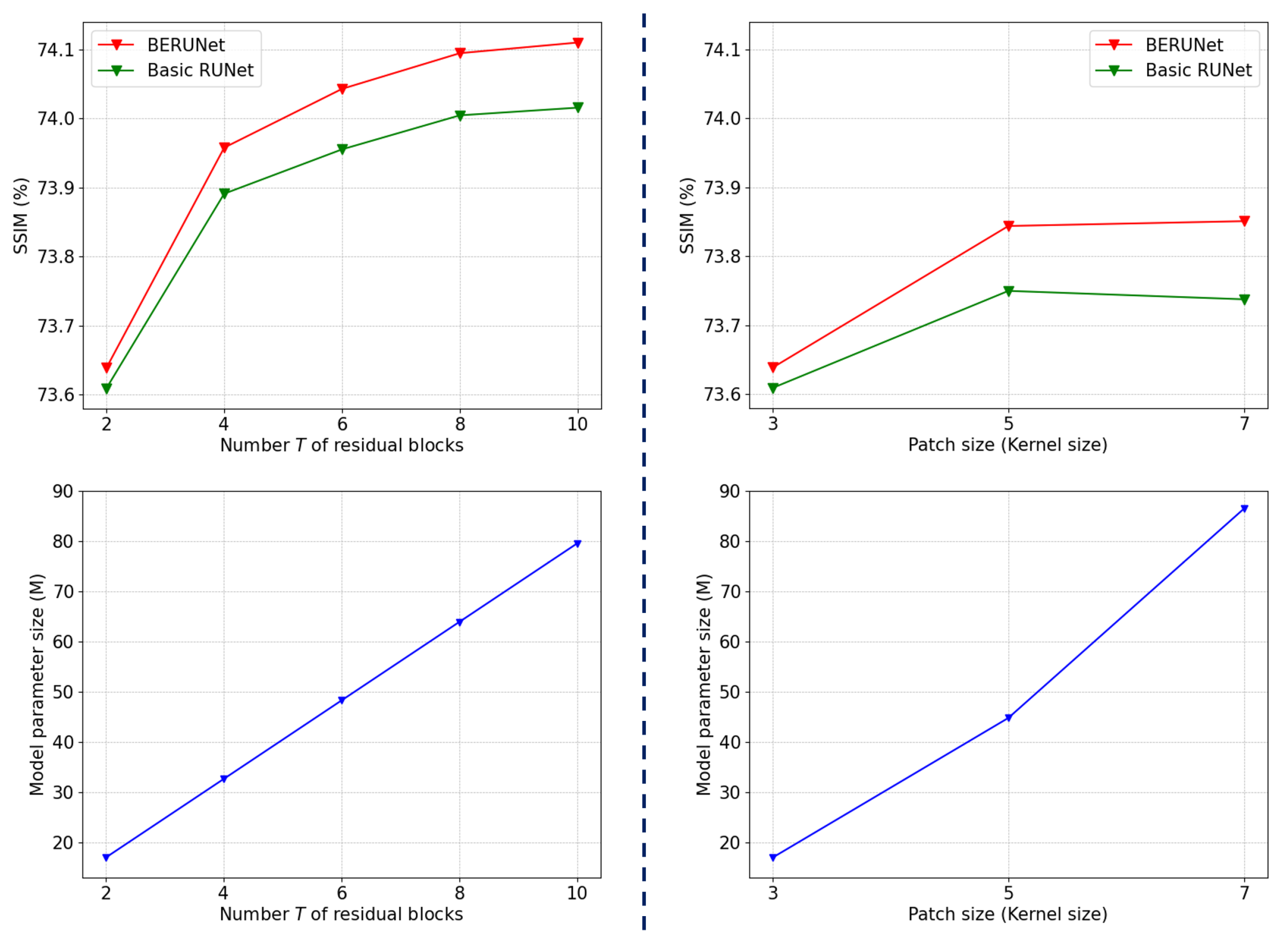
4.1.4. Selection of Architecture Hyperparameters for Image Denoising

Two hyperparameters affect the model’s denoising performance: (1) the number of stacked BERBlocks T in each encoder, decoder, and bottleneck module, which determines the depth of BERUNet; (2) the kernel size of Conv and TConv layers in each BERBlock (denoted as k), which corresponds to the patch size processed by the autoencoder in Section 3.2 and theoretically affects the ability of BERBlock to represent textures. We perform the ablation study on the BSD68 dataset with noise level $\sigma =50$. The results are illustrated in Figure 6, with basic RUNet used as a baseline for hyperparameter analysis.

Selection of T. We first fix $k=3$ and select T among $\left\{2,4,6,8,10\right\}$. It can be seen from the left side of Figure 6 that the SSIM index and parameter size of BERUNet increase with T. When $T=4$, BERUNet already exhibits a significant advantage in SSIM over the baseline. However, when $T>8,$ the improvement in SSIM becomes marginal. On the other hand, the training time, inference time, and parameter size continue to increase proportionally with T, leading to a linear decrease in computational efficiency. To balance performance and efficiency, we set $T=4$ for theoretical validation of BERUNet and $T=8$ for comparisons with other denoising methods.

Selection of k. We then fix $T=2$ and select k among $\left\{3,5,7\right\}$. The right side of Figure 6 plots the ablation study on k with the same vertical axis scale as the left side, which analyzes T, facilitating a unified discussion on the necessity of the k parameter. It can be seen that the SSIM index and parameter size of BERUNet also increase with k. However, the improvement in SSIM from increasing k is significantly smaller compared to increasing T, while the cost is a polynomial growth in parameter size with respect to k. To balance performance and efficiency, we set $k=3$ for BERUNet in the denoising task.

It is worth noting that regardless of increasing T or k, the performance advantage of BERUNet over basic RUNet becomes more pronounced. The possible reasons for this will be discussed in Section 4.2.3.

4.2. Impact of Enhancing Border Learning on Image Denoising

This section aims to verify whether the mask layer provides any advantage to BERBlock. To efficiently validate the theoretical properties of BERBlock in denoising while maintaining generality, the shallower version of BERUNet and its baseline methods (basic RUNet and TConv-based RUNet) were trained and analyzed.

4.2.1. Quantitative Analysis of the Denoising Metrics

As shown in Table 3 of Section 4.1.3, BERUNet outperforms basic RUNet and TConv-based RUNet in terms of average PSNR and SSIM across all test datasets. However, the improvements are marginal and not entirely convincing. To validate the effectiveness of enhancing border learning in improving denoising performance, we conducted paired t-tests between BERUNet and the baseline models across different datasets, with the p-values reported in

Table 4. T-test analysis of PSNR and SSIM between BERUNet and baseline models. Red indicates p-value < 0.05.

Methods	Padding/	Metrics	Set12			BSD68			Urban100
	Cropping		$\mathit{\sigma }=\mathit{15}$	$\mathit{\sigma }=\mathit{25}$	$\mathit{\sigma }=\mathit{50}$	$\mathit{\sigma }=\mathit{15}$	$\mathit{\sigma }=\mathit{25}$	$\mathit{\sigma }=\mathit{50}$	$\mathit{\sigma }=\mathit{15}$	$\mathit{\sigma }=\mathit{25}$	$\mathit{\sigma }=\mathit{50}$
BERUNet vs. TConv-based RUNet	✓	p-value of PSNR p-value of SSIM	0.268 0.018	0.520 0.026	0.159 0.007	0.269 <0.001	0.862 <0.001	0.043 <0.001	0.360 <0.001	0.279 <0.001	0.002 <0.001
	×	p-value of PSNR p-value of SSIM	0.337 0.012	0.429 0.032	0.294 0.033	0.024 0.001	0.086 0.004	0.031 0.013	<0.001 <0.001	0.026 0.008	0.058 0.019
BERUNet vs. basic RUNet	✓	p-value of PSNR p-value of SSIM	0.471 0.036	0.505 0.045	0.302 0.033	0.589 <0.001	0.883 <0.001	0.399 <0.001	0.115 <0.001	0.025 <0.001	0.005 <0.001

. Paired t-tests, commonly used in medical image processing for statistical hypothesis testing, confirm the reliability of performance improvement when $p<0.05$.

By analyzing Table 3 and Table 4 together, we can infer that the improvement in PSNR is somewhat associated with BERUNet. However, this correlation is unstable and may be influenced by the inherent randomness in DNN training and the constraints imposed by the L2 loss function on PSNR. On the other hand, the improvement in SSIM, which evaluates structural accuracy, is statistically significant, indicating that BERUNet more effectively captures texture structures.

4.2.2. Visualization Analysis of Feature Propagation Within DNN

Since PSNR and SSIM are global metrics computed over the entire image, they do not directly reveal the advantages introduced by BERUNet in reconstructing image textures. Therefore, we conducted further visual analyses from the perspectives of feature maps and denoising accuracy maps to more reliably validate the advantages of BERBlock in feature extraction and image denoising.

Figure 7 presents the feature maps, which are the mean of all channel feature maps output by the third scale, fourth residual block of the U-Net when denoising the ‘house’ image ($\sigma =0$). The five feature maps correspond to the five cases in Table 3. It can be clearly observed that, in padding-free CNN architectures, the feature maps output by the TConv-based RBlock exhibit weakened border features, while BERBlock effectively maintains the strength of the border features. When data padding is used, the TConv-based RBlock introduces ring-like artifacts, which are also present in the basic RBlock, whereas BERBlock only experiences a slight weakening of the border features. This suggests that the mask layer in BERBlock enhances its ability to learn border features, allowing image texture information to be more accurately propagated in the DNN. This successfully addresses the border effect problem mentioned in the introduction.

4.2.3. Visualization Analysis of Denoising Texture Accuracy

For the image denoising task, we focus more on the impact of BERBlock on the final denoising output of the DNN rather than on the internal feature maps. Figure 8 shows the average accuracy maps and relative accuracy maps for the five models in Table 3 on denoising the “house” image. For better analysis, the ground truth of the “house” image is also displayed on the left side of the second row. The first row of Figure 8 shows the average accuracy maps for different models, obtained by averaging the denoising accuracy maps over 1000 denoising instances of the “house“ image. In each denoising instance, Gaussian synthetic noise with $\sigma =50$ is randomly added to the “house” image. The accuracy map represents the pixel-wise denoising error e, defined as $e=\left|x_{\mathrm{est}}-x_{\mathrm{gt}}\right|$, where $x_{\mathrm{est}}$ is the model’s estimated denoised result and $x_{\mathrm{gt}}$ is the ground truth. A lower value of e indicates higher denoising accuracy, and in the average accuracy map, it is visualized in red. Interestingly, we found that no significant border effect was observed in the average accuracy map, and it is challenging to observe the differences between BERUNet and basic RUNet or TConv-based RUNet.

To more intuitively analyze the impact of BERUNet on denoising, we further calculated the relative accuracy maps of BERUNet compared to basic RUNet and BERUNet compared to TConv-based RUNet, which are shown on the right side of the second row in Figure 8. The relative accuracy map, denoted as r, is calculated via $r={\displaystyle \frac{{\overline{e}}_{\mathrm{BERUNet}}}{{\overline{e}}_{\mathrm{ref}}}}$, where ${\overline{e}}_{\mathrm{BERUNet}}$ represents the average accuracy map of BERUNet, and ${\overline{e}}_{\mathrm{ref}}$ represents the average accuracy map of the baseline method (basic RUNet or TConv-based RUNet). When BERUNet achieves higher denoising accuracy than the baseline methods, the value of r is less than 1 and is visualized in red in the relative accuracy map. Conversely, when BERUNet’s denoising accuracy is lower than that of the baseline methods, the value of r is greater than 1 and is visualized in blue in the relative accuracy map. From the relative accuracy map, we not only observe that BERUNet mitigates subtle boundary effects but also identify a tendency for BERUNet and basic RUNet (or TConv-based RUNet) to reconstruct different textures during denoising. Specifically, BERUNet more accurately restores high-frequency textures, while basic RUNet (or TConv-based RUNet) is more adept at estimating mid-frequency textures. This explains why, as shown in Table 3 and Table 4, the PSNR improvement of BERUNet over TConv-based RUNet or basic RUNet is limited, but the SSIM improvement is more significant.

A comprehensive analysis of the feature maps in Section 4.2.2 and denoising accuracy maps in this subsection suggests that, under the constraint of the loss function, the border effects in the front basic RBlocks (or TConv-based RBlocks) within the stacked residual block-based DNN architecture are partially corrected by subsequent residual blocks. As a result, the border effect in the final output of the DNN is weak and nearly invisible. However, the severe border effect in the internal feature maps of the DNN, on one hand, transmits invalid high-frequency information, and on the other hand, aliases valid high-frequency information, thereby interfering with the DNN’s ability to learn and infer high-frequency textures. Thus, although the motivation behind the proposed BERUNet is to enhance the learning of border features, it ultimately impacts the restoration accuracy of high-frequency textures across the entire image. Based on this observation, using conventional PSNR and SSIM metrics to evaluate the denoising performance of BERUNet remains feasible. This also provides a strong explanation for the differences in the SSIM metric variation with T and k between BERUNet and the baseline methods observed in Section 4.1.4.

4.3. Comparison with Advanced DNN-Based Denoising Methods

In this section, we train a deeper version of BERUNet and compare its performance with 19 advanced methods based on different DNN architectures for grayscale synthetic noise, color synthetic noise, and real-world noise removal on the benchmark datasets Set12, BSD68, Kodak24, McMaster, Urban100, and SIDD. This comparison aims to discuss the advantages and limitations of the proposed method.

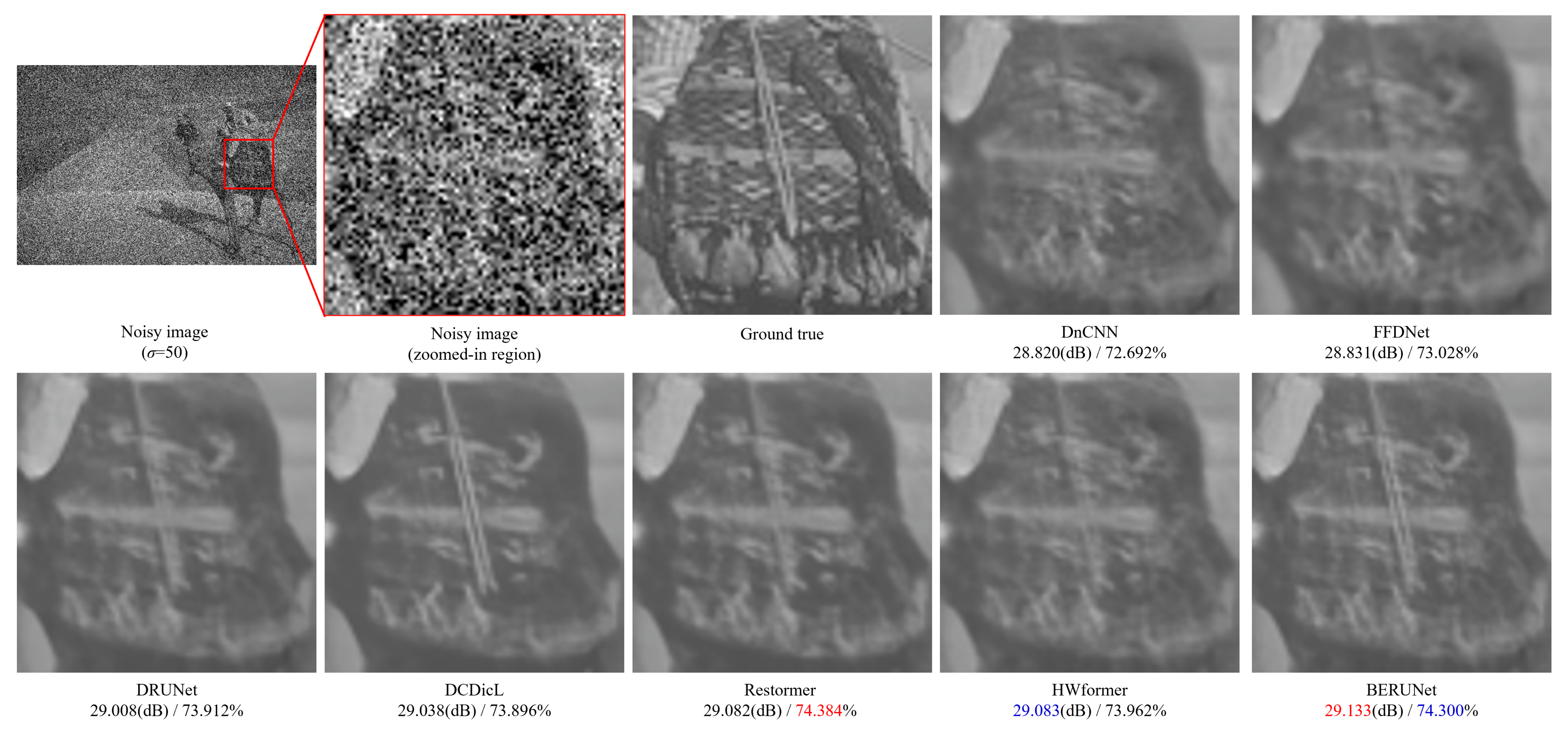
4.3.1. Removal of Grayscale Synthetic Noise

For grayscale image denoising, we compared the proposed BERUNet denoiser with several DNN-based denoising methods, including five methods which separately learn a single model for each noise level (i.e., DnCNN [1], DAGL [84], SwinIR [11], CTNet [85], and HWformer [86]) and five methods which were trained to handle a wide range of noise levels (i.e., IRCNN [87], FFDNet [88], DCDicL [14], DRUNet [4], and Restormer).These methods represent three of the most advanced and effective denoising DNN architectures: FCN, U-Net, and Transformer. The test codes and trained models of these benchmark methods are released by their authors. We evaluated them in a Python environment using the same testing settings to ensure a fair comparison.

The denoising performance of different methods on the three grayscale image datasets are reported in

Table 5. Average PSNR and SSIM for removing grayscale synthetic noise using different methods. Red and blue indicate the highest and second-highest values, respectively.

Methods	Primary	Metrics	Set12			BSD68			Urban100
	Architecture		$\mathit{\sigma }=\mathit{15}$	$\mathit{\sigma }=\mathit{25}$	$\mathit{\sigma }=\mathit{50}$	$\mathit{\sigma }=\mathit{15}$	$\mathit{\sigma }=\mathit{25}$	$\mathit{\sigma }=\mathit{50}$	$\mathit{\sigma }=\mathit{15}$	$\mathit{\sigma }=\mathit{25}$	$\mathit{\sigma }=\mathit{50}$
DnCNN (2017)	FCN	PSNR (dB) SSIM (%)	32.851 90.251	30.432 86.166	27.169 78.277	31.722 88.996	29.222 82.712	26.233 71.802	32.643 92.406	29.945 87.806	26.263 78.565
IRCNN (2017)	FCN	PSNR (dB) SSIM (%)	32.759 90.059	30.371 85.979	27.124 78.043	31.621 88.752	29.138 82.403	26.181 71.613	32.463 92.360	29.803 88.311	26.223 79.184
FFDNet (2018)	FCN	PSNR (dB) SSIM (%)	32.739 90.242	30.419 86.313	27.300 78.994	31.623 88.952	29.183 82.803	26.289 72.306	32.405 92.648	29.903 88.785	26.503 80.475
DCDicL (2021)	Unfolding network + U-Net	PSNR (dB) SSIM (%)	33.341 91.152	31.026 87.478	27.999 81.216	31.922 89.486	29.492 83.690	26.613 73.836	33.595 93.881	31.304 91.079	28.236 85.483
DAGL (2021)	FCN + NLNN	PSNR (dB) SSIM (%)	33.272 91.002	30.926 87.198	27.793 80.421	31.912 89.449	29.457 83.547	26.524 73.198	33.748 93.860	31.363 90.835	27.954 84.081
SwinIR (2021)	FCN + Transformer	PSNR (dB) SSIM (%)	33.377 91.108	31.037 87.431	27.956 81.017	31.948 89.534	29.494 83.698	26.582 73.721	33.726 93.911	31.339 90.953	28.060 84.764
DRUNet (2022)	U-Net	PSNR (dB) SSIM (%)	33.245 90.980	30.936 87.327	27.896 80.962	31.886 89.449	29.455 83.633	26.569 73.721	33.442 93.761	31.109 90.820	27.963 84.830
Restormer (2022)	U-Net + Transformer	PSNR (dB) SSIM (%)	33.346 91.150	31.042 87.535	28.006 81.209	31.947 89.561	29.521 83.831	26.639 74.103	33.671 93.889	31.393 91.095	28.332 85.551
CTNet (2024)	Parallel Network + Transformer	PSNR (dB) SSIM (%)	33.322 91.001	30.959 87.240	27.802 80.386	31.922 89.456	29.456 83.516	26.492 73.063	33.693 93.824	31.256 90.720	27.790 83.713
HWformer (2024)	FCN + Transformer	PSNR (dB) SSIM (%)	33.424 91.233	31.075 87.532	27.979 81.045	31.978 89.589	29.534 83.791	26.611 73.745	33.909 94.060	31.591 91.266	28.332 85.261
BERUNet (Ours)	U-Net	PSNR (dB) SSIM (%)	33.347 91.169	31.051 87.555	28.033 81.294	31.944 89.570	29.522 83.846	26.651 74.095	33.609 93.894	31.387 91.216	28.267 85.501

. It can be seen that BERUNet achieves highly competitive performance. Specifically, first, BERUNet achieves the best performance among simple FCN-based and U-Net-based methods. Second, its performance is comparable to state-of-the-art methods that incorporate Transformer blocks. Finally, BERUNet excels in restoring image texture structures, as reflected in its superior SSIM performance. It is noteworthy that HWformer slightly outperforms BERUNet in most scenarios. This advantage not only stems from the use of Transformer blocks in the primary architecture but also from training separate models for different noise levels. In contrast, BERUNet handles various noise levels using a single model.

Figure 9 and Figure 10 show the visual denoising results of the seven representative methods from Table 5 on image 60 from the BSD68 dataset and image 038 from the Urban100 dataset, respectively. The zoomed-in views of test images are shown for detailed comparison. It can be observed that although BERUNet did not achieve the best performance in PSNR and SSIM, it generates richer textures and more refined edges.

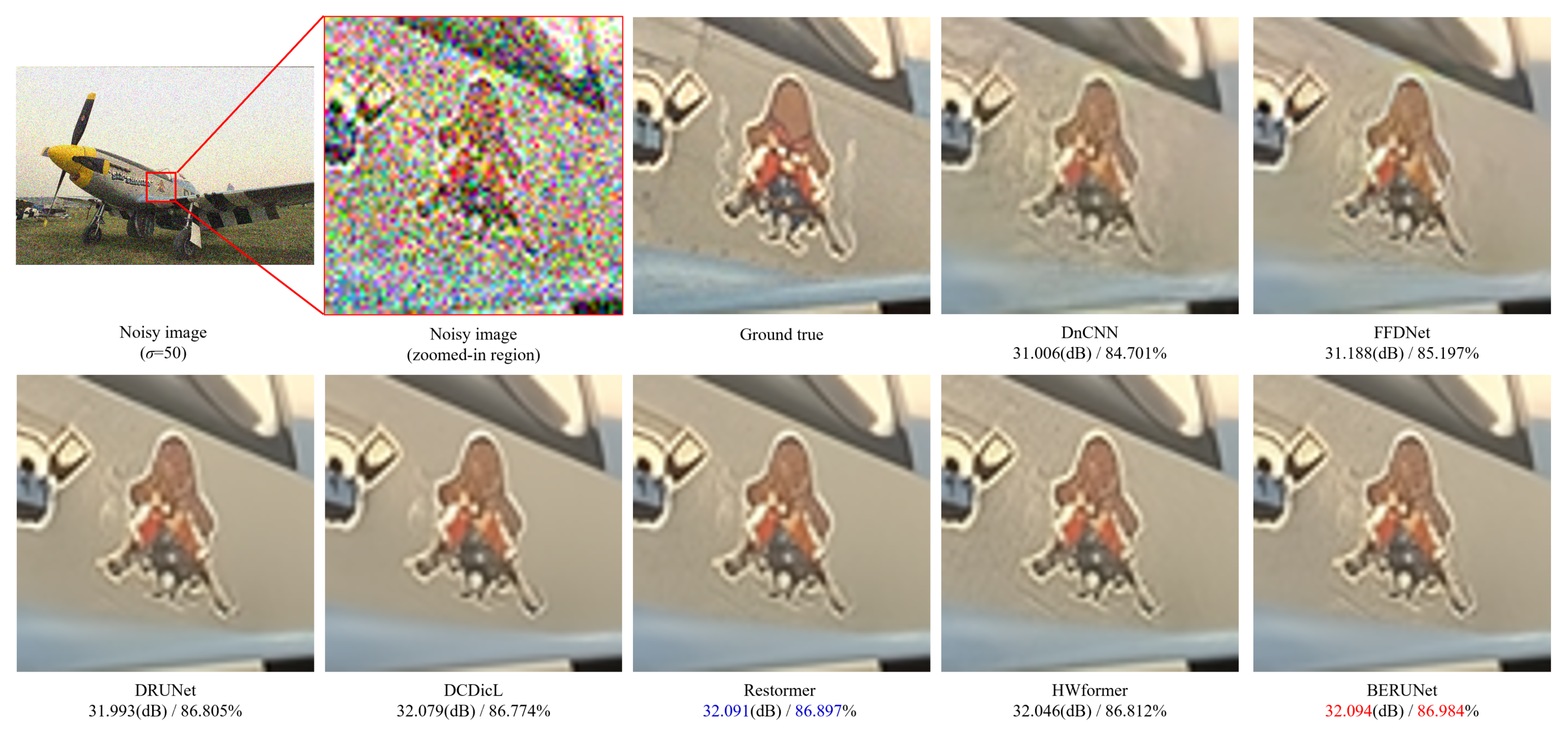
4.3.2. Removal of Color Synthetic Noise

For color image denoising, we further evaluated the performance of BERUNet by comparing it with four methods that train a separate model for each noise level (i.e., BRDNet [89], SwinIR, CTNet, and HWformer) and six methods trained to handle various noise levels (i.e., DnCNN, IRCNN, FFDNet, DCDicL, DRUNet, and Restormer). The released testing code and pretrained models for these methods support color image denoising.

The denoising performance of different methods on four color image datasets is reported in

Table 6. Average PSNR and SSIM for removing color synthetic noise using different methods. Red and blue indicate the highest and second-highest values, respectively.

	Primary	Metrics	CBSD68			Kodak24			McMaster			Urban100
Methods	Architecture		$\mathit{\sigma }=\mathit{15}$	$\mathit{\sigma }=\mathit{25}$	$\mathit{\sigma }=\mathit{50}$	$\mathit{\sigma }=\mathit{15}$	$\mathit{\sigma }=\mathit{25}$	$\mathit{\sigma }=\mathit{50}$	$\mathit{\sigma }=\mathit{15}$	$\mathit{\sigma }=\mathit{25}$	$\mathit{\sigma }=\mathit{50}$	$\mathit{\sigma }=\mathit{15}$	$\mathit{\sigma }=\mathit{25}$	$\mathit{\sigma }=\mathit{50}$
DnCNN (2017)	FCN	PSNR (dB) SSIM (%)	33.898 92.903	31.244 88.300	27.946 78.963	34.596 92.089	32.136 87.753	28.948 79.173	33.450 90.353	31.521 86.942	28.620 79.856	32.984 93.143	30.811 90.148	27.589 83.308
IRCNN (2017)	FCN	PSNR (dB) SSIM (%)	33.872 92.845	31.179 88.238	27.879 78.978	34.689 92.093	32.150 87.793	28.936 79.426	34.577 91.949	32.182 88.176	28.928 80.692	33.777 94.017	31.204 90.878	27.701 83.959
FFDNet (2018)	FCN	PSNR (dB) SSIM (%)	33.879 92.896	31.220 88.211	27.974 78.871	34.749 92.243	32.250 87.912	29.109 79.524	34.656 92.158	32.359 88.614	29.194 81.494	33.834 94.182	31.404 91.201	28.054 84.764
BRDNet (2020)	Parallel Network + FCN	PSNR (dB) SSIM (%)	34.103 92.909	31.431 88.470	28.157 79.423	34.878 92.492	32.407 88.560	29.215 80.401	35.077 92.691	32.745 89.433	29.520 82.649	34.421 94.616	31.993 91.941	28.556 85.769
DCDicL (2021)	Unfolding network + U-Net	PSNR (dB) SSIM (%)	34.335 93.468	31.728 89.289	28.551 81.040	35.385 92.999	32.972 89.275	29.960 82.190	35.483 93.328	33.238 90.454	30.200 84.906	34.903 95.111	32.771 92.998	29.875 88.838
SwinIR (2021)	FCN + Transformer	PSNR (dB) SSIM (%)	34.410 93.557	31.773 89.403	28.561 81.199	35.464 93.045	33.008 89.316	29.947 82.208	35.609 93.454	33.311 90.558	30.198 84.896	35.162 95.234	32.934 93.051	29.876 88.607
DRUNet (2022)	U-Net	PSNR (dB) SSIM (%)	34.287 93.435	31.676 89.247	28.494 81.029	35.312 92.918	32.894 89.171	29.869 82.075	35.392 93.245	33.131 90.306	30.069 84.604	34.826 95.054	32.609 92.826	29.611 88.348
Restormer (2022)	U-Net + Transformer	PSNR (dB) SSIM (%)	34.386 93.539	31.780 89.419	28.608 81.340	35.440 93.044	33.023 89.361	30.002 82.346	35.541 93.385	33.299 90.563	30.276 85.160	35.056 95.188	32.906 93.077	30.016 88.937
CTNet (2024)	Parallel Network + Transformer	PSNR (dB) SSIM (%)	34.374 93.490	31.716 89.249	28.455 80.745	35.395 92.963	32.915 89.147	29.782 81.702	35.544 93.308	33.221 90.281	30.038 84.130	35.119 95.172	32.859 92.915	29.733 88.214
HWformer (2024)	FCN + Transformer	PSNR (dB) SSIM (%)	34.412 93.546	31.784 89.386	28.580 81.191	35.483 93.076	33.037 89.376	29.959 82.243	35.641 93.461	33.362 90.570	30.240 84.818	35.261 95.293	33.100 93.191	30.139 88.981
BERUNet (Ours)	U-Net	PSNR (dB) SSIM (%)	34.394 93.563	31.782 89.460	28.596 81.365	35.447 93.080	33.036 89.438	29.981 82.390	35.592 93.449	33.290 90.569	30.262 85.004	35.114 95.221	32.903 93.102	29.996 88.956

. BERUNet’s performance in color image denoising is consistent with its performance in grayscale image denoising. The performance of BERUNet outperforms simple FCN-based and U-Net-based methods and is comparable to state-of-the-art Transformer-based methods.

Similarly, the visual denoising results of the seven representative methods from Table 6 on the image kodim20 from the Kodak24 dataset and image 054 from the Urban100 dataset are shown in Figure 11 and Figure 12, respectively. It can be observed that simple CNN-based methods (DnCNN, IRCNN, FFDNet, DRUNet) can restore more diverse textures but tend to generate ring-like artifacts. In contrast, Transformer-based methods (Restormer and HWformer) and unfolded sparse coding methods (DCDicL) tend to restore structurally regular textures but smooth out irregular textures. BERUNet strikes a balance between the two, achieving higher PSNR and SSIM metrics.

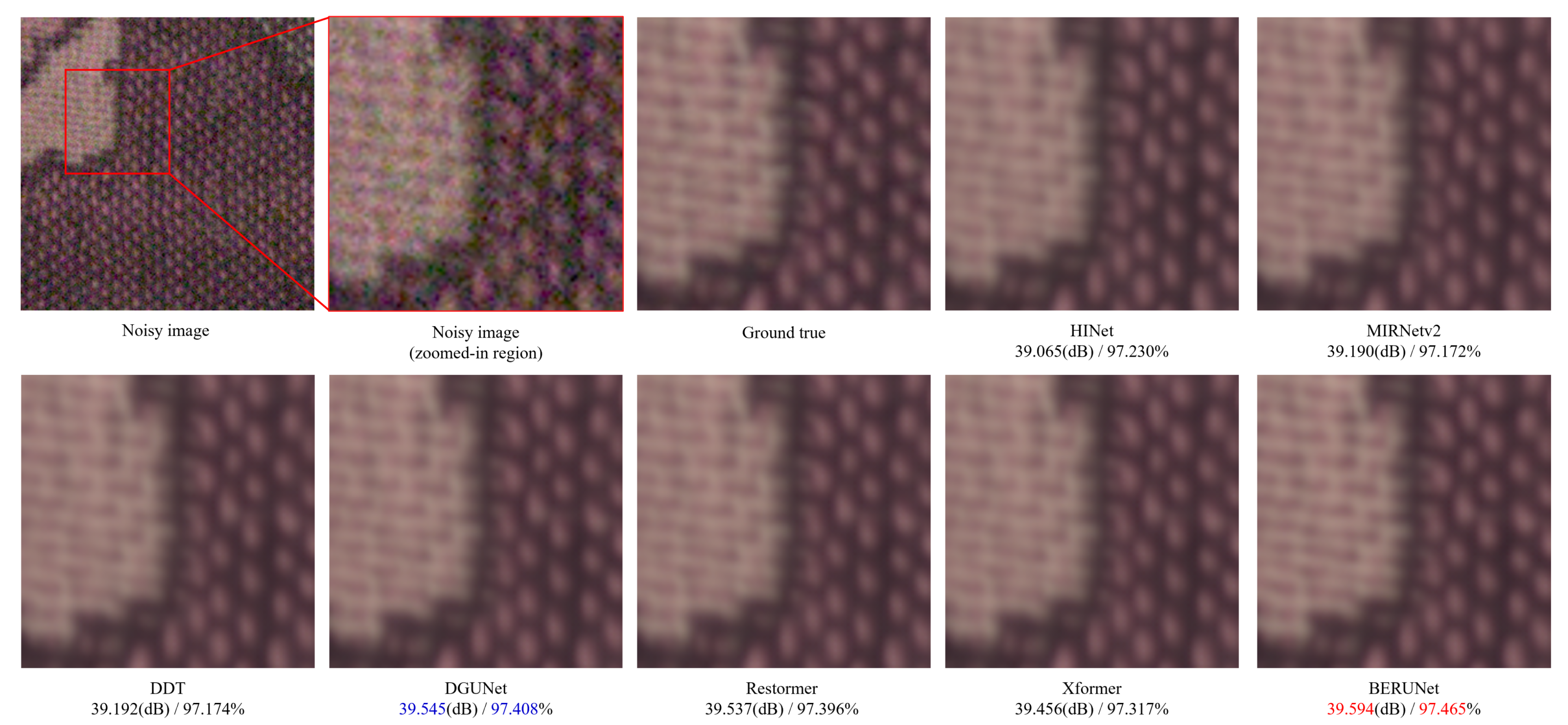
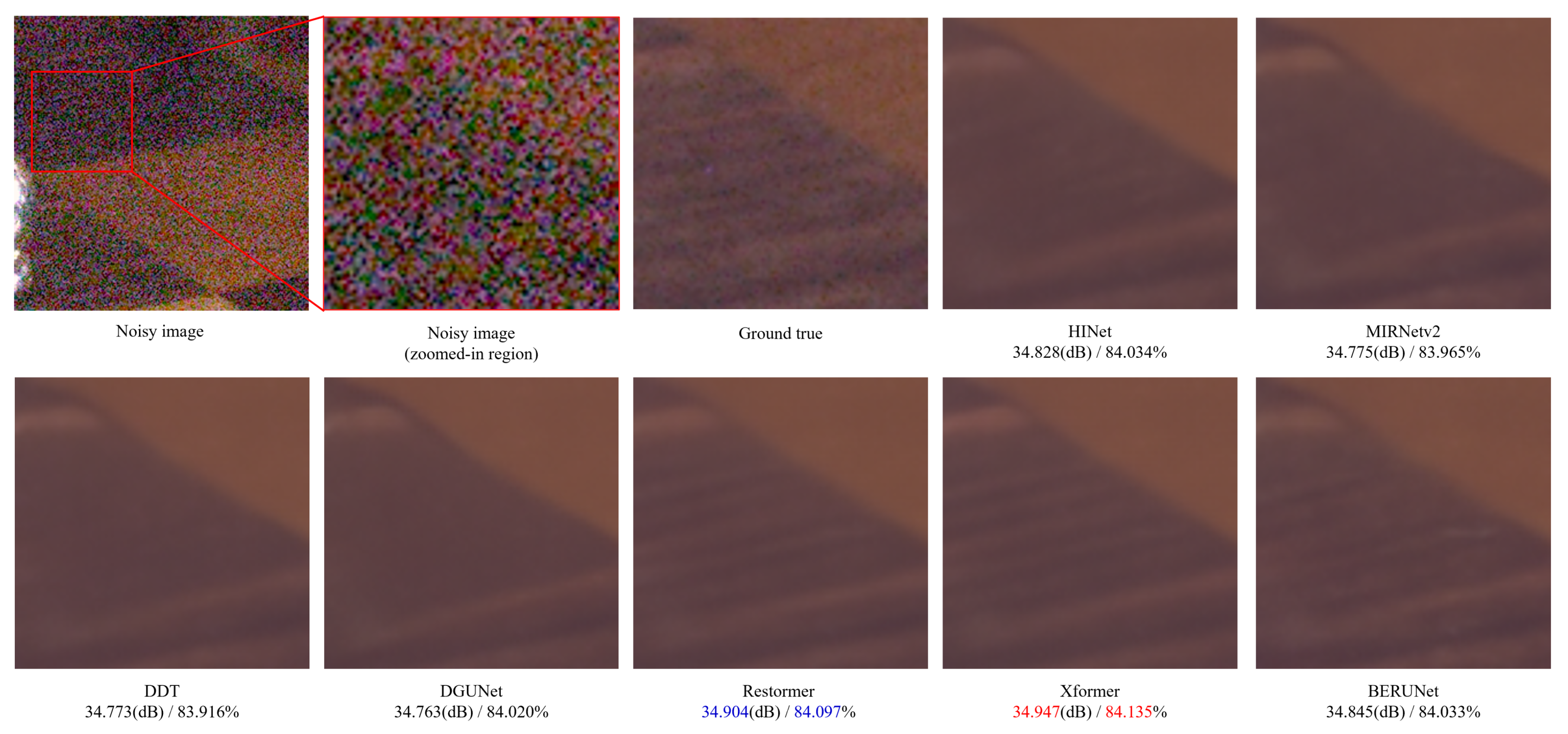
4.3.3. Removal of Real-World Noise

This section will validate the effectiveness of BERUNet in removing real-world noise. Figure 5 illustrates the BERUNet architecture for non-blind denoising, which is more suitable for synthetic noise with known noise levels. However, in real-world scenarios, the noise model and noise level are unknown. Therefore, we remove the input noise level map and train a blind denoising model on the SIDD dataset. We evaluated the performance of BERUNet on the SIDD validation data and compared it with ten state-of-the-art representative methods, including CycleISP [90], HINet [91], MPRNet [92], Restormer, DGUNet+ [15], MIRNetv2 [93], DDT [94], CTNet, DRANet [3], and Xformer [95]. These methods have generated test codes and pre-trained models for real-world denoising which have been presented by their original authors.

The denoising performance of different methods on the SIDD dataset is reported in

Table 7. Average PSNR and SSIM for denoising SIDD dataset using different methods. Red, blue, and cyan indicate the highest, second-highest, and third-highest values, respectively.

Methods	CycleISP (2020)	HINet (2021)	MPRNet (2021)	Restormer (2022)	DGUNet+ (2022)	MIRNetv2 (2022)	DDT (2023)	CTNet (2024)	DRANet (2024)	Xformer (2024)	BERUNet (Ours)
Primary architecture	FCN + NLNN	Multi-stage FCN	Multi-stage U-Net	U-Net + Transformer	Unfolding network + U-Net	FCN + UNet + Transformer	U-Net + Transformer	Parallel Network + Transformer	Parallel Network + FCN	U-Net + Transformer	U-Net
PSNR (dB) SSIM (%)	39.439 91.744	39.776 92.017	39.630 91.957	39.929 92.146	39.800 92.064	39.757 92.005	39.749 92.010	38.377 90.475	39.427 91.796	39.891 92.154	39.847 92.119

. BERUNet’s performance in denoising real noisy images is not as strong as its performance on synthetic noisy images. However, as a simple U-Net architecture model, BERUNet’s denoising performance outperforms most more sophisticated methods, especially considering that the SSIM metric is very close to that of state-of-the-art Transformer-based methods. This is sufficient to demonstrate that the proposed BERBlock is effective for denoising tasks.

The visual denoising results of the seven representative methods from Table 7 on image 36_27 and 18_15 from the SIDD validation data are shown in Figure 13 and Figure 14. These two images represent scenarios where BERUNet demonstrates its strengths and weaknesses, respectively. In the test on image 36_27, BERUNet achieved the highest PSNR and SSIM due to its ability to restore sharper texture edges. However, in the test on image 18_15, although BERUNet also recovered rich texture details, its PSNR and SSIM were lower than those of Transformer-based methods such as Restormer and Xformer.

A closer examination of the texture differences between images 36_27 and 18_15 reveals that the ground truth of 36_27 is relatively clean and retains complete textures, while the ground truth of 18_15 still exhibits residual noise effects, leading to discontinuous textures. In BERUNet’s denoised result for 18_15, the restored texture tends to be fragmented, whereas Restormer and Xformer tend to “infer” a more continuous texture structure. Interestingly, we observed that the variation in BERUNet’s performance across different images is highly consistent with DGUNet+, as both models rely solely on a CNN-based U-Net architecture without incorporating Transformers. This suggests that the observed differences in texture restoration may stem from the ability of Transformers to capture non-local information.

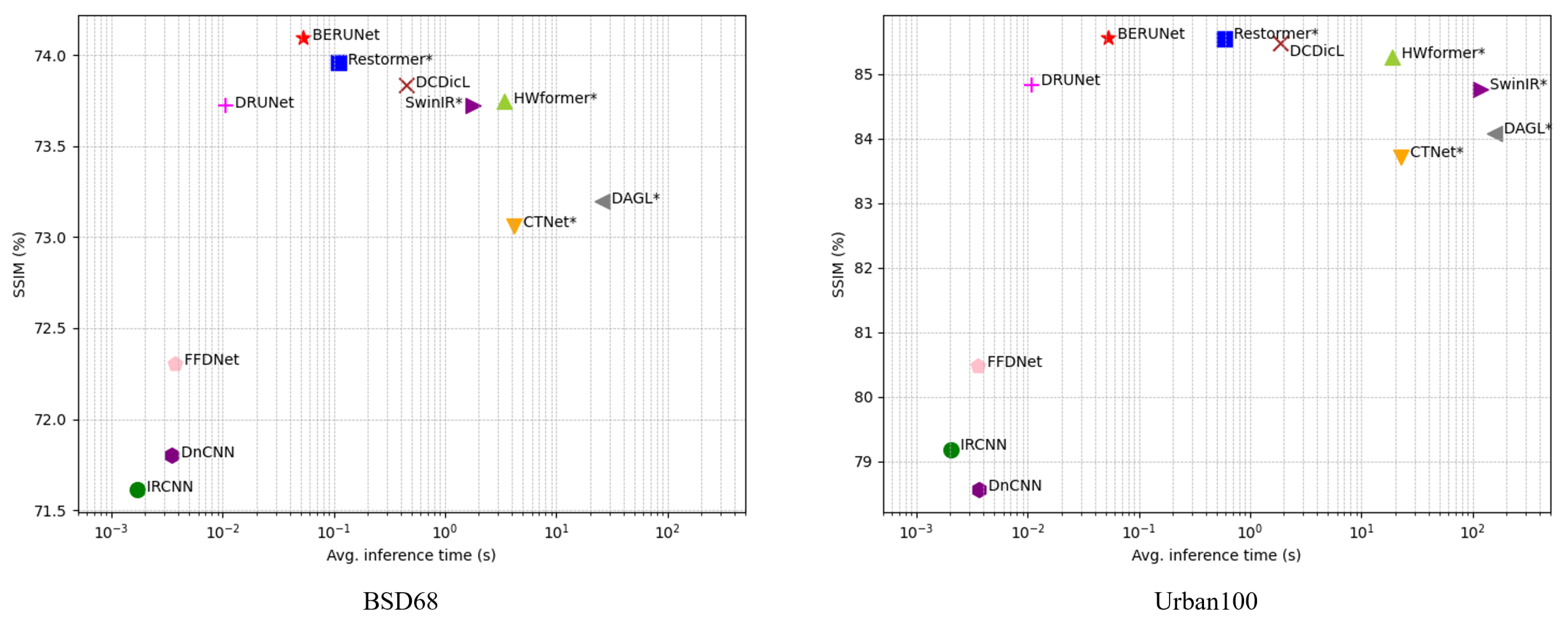
4.3.4. Advantages of BERUNet in Fast Denoising

In many cases, the goal of denoising tasks is not to achieve the clearest image, but to process it as quickly as possible while maintaining sufficient clarity, given the constraints of limited computational resources. Previous experiments have demonstrated that the proposed BERBlock enables a simple U-Net architecture to achieve highly competitive performance. This section will prove that BERUNet also leads in inference speed.

In this case, the inference times of the methods listed in Table 5 were compared on the BSD68 and Urban100 datasets. The BSD68 dataset consists of images with a uniform size of 321 × 481, reflecting the average inference time for stable, smaller-sized images. On the other hand, the Urban100 dataset includes images with varying sizes, where the longer side of the images has 1024 pixels, reflecting the average inference time for larger, more variable images. Synthetic noise with $\sigma =50$ was added to the datasets, and inference was performed using an Nvidia Titan V GPU. Each dataset was tested three times, and the shortest average inference time was recorded.

As shown in Figure 15, the SSIM indices and inference speeds of different methods are compared. According to its deeper network architecture and larger model size, BERUNet achieves the best performance but the longest inference time among the CNN-based methods (DnCNN, IRCNN, FFDNet, DRUNet). However, when compared to Transformer-based networks (DAGL, SwinIR, CTNet, HWformer, and Restormer) and unfolding networks (DCDicL), BERUNet achieves a significant advantage in inference speed, while maintaining comparable performance. This advantage becomes even more pronounced when denoising the Urban100 dataset. Specifically, BERUNet achieves an average inference time of 0.05 s for both BSD68 and Urban100, meeting real-time requirements. In contrast, the fastest Transformer-based DNN (Restormer) has an average inference time of 0.58 s on Urban100, while the slowest Transformer-based DNN (DAGL) takes up to 3 min on Urban100. Overall, we can conclude that BERUNet provides an excellent solution in terms of both effectiveness and efficiency.

4.3.5. Limitations of BERUNet in Image Denoising Task

In our experiments, we observed that BERUNet exhibits advantages in restoring high-frequency textures and achieving fast denoising. However, it also presents certain limitations in terms of generalization capability and unsupervised learning.

Limitations in generalization capability. In synthetic Gaussian noise removal tests, BERUNet outperformed Restormer and HWformer in terms of SSIM scores on the Set12, BSD68, and Kodak24 datasets. However, its performance was relatively weaker for the McMaster and Urban100 datasets. In real-world noise removal tests, BERUNet demonstrated strong high-frequency texture restoration for images with clean ground truth. However, for images where the ground truth textures were partially missing, BERUNet tended to restore only visible textures, whereas Restormer and Xformer attempted to generate complete and continuous textures.

These findings indicate that BERUNet’s denoising performance is significantly influenced by the texture characteristics of the training dataset and the noise model. To achieve state-of-the-art denoising performance, it is necessary to train separate models for different types of noise (e.g., Gaussian, Poisson, real-world noise) and different datasets (e.g., natural images, CT images, hyperspectral images, infrared images), ensuring that the ground truth images in the training set are sufficiently clean. Given that Restormer, HWformer, and Xformer incorporate Transformer modules, we attribute BERUNet’s limitations to its inherent nature as a CNN-based model derived from a patch-wise autoencoder. Unlike Transformer-based models, which introduce self-attention mechanisms or non-local texture correlation assumptions, BERUNet does not impose additional explicit assumptions on noise or image structures, leading to its relatively weaker generalization capability.

Limitations in unsupervised/self-supervised learning. This study focuses on addressing the border effects caused by zero padding in Conv layers of deep neural networks (DNNs) and analyzing how these effects influence the denoising performance of DNNs. Therefore, we trained BERUNet solely under supervised learning conditions to investigate the theoretical properties and denoising performance of BERBlock. This choice is both reasonable and sufficient, and thus, no specific optimization for unsupervised or self-supervised learning was conducted in this work.

Considering that BERUNet is a CNN based on the U-Net architecture, it can be adapted for unsupervised, semi-supervised, or self-supervised training using frameworks such as GANs [96,97] or blind-spot networks [98,99]. Beyond these conventional approaches, it is noteworthy that the autoencoder used to interpret BERBlock is inherently an unsupervised model and is often designed for semi-supervised or self-supervised learning [100,101]. This implies that by incorporating autoencoder-related techniques and applying regularization constraints on BERBlock’s weights and hidden layers, BERUNet can improve its generalization ability while also having the potential to be trained in an unsupervised or self-supervised manner. However, these improvements fall outside the motivation of this study and are not further explored in this work.

5. Conclusions

To address the border effects generated by consecutive convolutions in existing CNNs, we propose a novel CNN residual block architecture derived from patch-based DNNs, called the Border-Enhanced Residual Block (BERBlock). By stacking BERBlocks into BERUNet, we demonstrate its effectiveness in image denoising. BERBlock follows the mathematical principles of patch-based methods, utilizing a patch-wise autoencoder in DNNs to learn image-wise mappings. Since matrix operations on patches can be accelerated by Conv and TConv layers, BERBlock is regarded as a new CNN architecture. It incorporates a mask to enhance border features, effectively mitigating the ring-like border artifacts caused by zero padding in convolutional layers. This ensures that the high-frequency information propagated through BERUNet remains unaffected, ultimately improving the accuracy of high-frequency texture restoration in the output image.

Experiments on synthetic Gaussian noise removal using the benchmark datasets Set12, BSD68, Kodak24, McMaster, and Urban100, as well as real-world noise removal on the SIDD dataset, demonstrate that BERUNet outperforms previous FCN- and U-Net-based methods in both quantitative metrics (PSNR and SSIM) and high-frequency texture preservation in visual quality. Its performance is comparable to, and in some cases even surpasses, state-of-the-art Transformer-based methods, while also exhibiting a significant advantage in inference speed. The proposed architecture is grounded in rigorous mathematical derivations, providing valuable insights into the underlying mechanisms of CNNs.

In addition to the aforementioned advantages, we also discussed the limitations of BERUNet in terms of generalization ability and unsupervised/self-supervised learning. Therefore, future work will focus on three key directions: (1) applying the proposed BERBlock to the design of other network architectures; (2) incorporating regularization constraints on the parameters and hidden layers of BERUNet to improve its generalization ability; and (3) exploring unsupervised/self-supervised training methods for BERUNet based on autoencoder theory. Across all these directions, the primary goal is to optimize the denoising performance of DNNs by analyzing and enhancing the ability of convolutional layers to learn image features.

References

1. Zhang, K.; Zuo, W.; Chen, Y.; Meng, D.; Zhang, L. Beyond a gaussian denoiser: Residual learning of deep cnn for image denoising. IEEE Trans. Image Process. 2017, 26, 3142–3155. [Google Scholar] [CrossRef] [PubMed]
2. Tai, Y.; Yang, J.; Liu, X.; Xu, C. Memnet: A persistent memory network for image restoration. In Proceedings of the IEEE International Conference on Computer Vision, Venice, Italy, 22–27 October 2017; pp. 4539–4547. [Google Scholar]
3. Wu, W.; Liu, S.; Xia, Y.; Zhang, Y. Dual residual attention network for image denoising. Pattern Recognit. 2024, 149, 110291. [Google Scholar] [CrossRef]
4. Zhang, K.; Li, Y.; Zuo, W.; Zhang, L.; Van Gool, L.; Timofte, R. Plug-and-play image restoration with deep denoiser prior. IEEE Trans. Pattern Anal. Mach. Intell. 2021, 44, 6360–6376. [Google Scholar] [CrossRef] [PubMed]
5. Wu, Z.; Li, J.; Xu, C.; Huang, D.; Hoi, S.C. RUN: Rethinking the UNet Architecture for Efficient Image Restoration. IEEE Trans. Multimed. 2024, 26, 10381–10394. [Google Scholar] [CrossRef]
6. Cheng, J.; Liang, D.; Tan, S. Transfer CLIP for Generalizable Image Denoising. In Proceedings of the IEEE/CVF Conference on Computer Vision and Pattern Recognition, Seattle, WA, USA, 17–21 June 2024; pp. 25974–25984. [Google Scholar]
7. Liu, D.; Wen, B.; Fan, Y.; Loy, C.C.; Huang, T.S. Non-local recurrent network for image restoration. In Proceedings of the 32nd Conference on Neural Information Processing Systems (NeurIPS), Montréal, QC, Canada, 3–8 December 2018; Curran Associates, Inc.: Red Hook, NY, USA, 2018; Volume 31. [Google Scholar]
8. Yan, Q.; Zhang, L.; Liu, Y.; Zhu, Y.; Sun, J.; Shi, Q.; Zhang, Y. Deep HDR imaging via a non-local network. IEEE Trans. Image Process. 2020, 29, 4308–4322. [Google Scholar] [CrossRef]
9. Sehgal, R.; Kaushik, V.D. Deep Residual Network and Wavelet Transform-Based Non-Local Means Filter for Denoising Low-Dose Computed Tomography. Int. J. Image Graph. 2024, 2550072. [Google Scholar] [CrossRef]
10. Liu, H.; Li, X.; Cheng, Z.; Liu, T.; Zhai, J.; Hu, H. Polarimetric image denoising via non-local based cube matching convolutional neural network. Opt. Lasers Eng. 2025, 184, 108684. [Google Scholar] [CrossRef]
11. Liang, J.; Cao, J.; Sun, G.; Zhang, K.; Van Gool, L.; Timofte, R. Swinir: Image restoration using swin transformer. In Proceedings of the IEEE/CVF International Conference on Computer Vision, Montreal, BC, Canada, 11–17 October 2021; pp. 1833–1844. [Google Scholar]
12. Yan, Q.; Liu, S.; Xu, S.; Dong, C.; Li, Z.; Shi, J.Q.; Zhang, Y.; Dai, D. 3D Medical image segmentation using parallel transformers. Pattern Recognit. 2023, 138, 109432. [Google Scholar] [CrossRef]
13. Zhang, S.Y.; Wang, Z.X.; Yang, H.B.; Chen, Y.L.; Li, Y.; Pan, Q.; Wang, H.K.; Zhao, C.X. Hformer: Highly efficient vision transformer for low-dose CT denoising. Nucl. Sci. Tech. 2023, 34, 61. [Google Scholar] [CrossRef]
14. Zheng, H.; Yong, H.; Zhang, L. Deep convolutional dictionary learning for image denoising. In Proceedings of the IEEE/CVF Conference on Computer Vision and Pattern Recognition, Nashville, TN, USA, 20–25 June 2021; pp. 630–641. [Google Scholar]
15. Mou, C.; Wang, Q.; Zhang, J. Deep generalized unfolding networks for image restoration. In Proceedings of the IEEE/CVF Conference on Computer Vision and Pattern Recognition, New Orleans, LA, USA, 18–24 June 2022; pp. 17399–17410. [Google Scholar]
16. Xu, W.; Zhu, Q.; Qi, N.; Chen, D. Deep sparse representation based image restoration with denoising prior. IEEE Trans. Circuits Syst. Video Technol. 2022, 32, 6530–6542. [Google Scholar] [CrossRef]
17. Ulyanov, D.; Vedaldi, A.; Lempitsky, V. Deep image prior. In Proceedings of the IEEE Conference on Computer Vision and Pattern Recognition, Salt Lake City, UT, USA, 18–23 June 2018; pp. 9446–9454. [Google Scholar]
18. Tran, L.D.; Nguyen, S.M.; Arai, M. GAN-based noise model for denoising real images. In Proceedings of the Asian Conference on Computer Vision, Kyoto, Japan, 30 November–4 December 2020. [Google Scholar]
19. Niu, C.; Li, K.; Wang, D.; Zhu, W.; Xu, H.; Dong, J. Gr-gan: A unified adversarial framework for single image glare removal and denoising. Pattern Recognit. 2024, 156, 110815. [Google Scholar]
20. Kawar, B.; Elad, M.; Ermon, S.; Song, J. Denoising diffusion restoration models. In Proceedings of the 36th Conference on Neural Information Processing Systems (NeurIPS 2022), New Orleans, LO, USA, 28 November–9 December 2022; Volume 35, pp. 23593–23606. [Google Scholar]
21. Zeng, H.; Cao, J.; Zhang, K.; Chen, Y.; Luong, H.; Philips, W. Unmixing Diffusion for Self-Supervised Hyperspectral Image Denoising. In Proceedings of the IEEE/CVF Conference on Computer Vision and Pattern Recognition, Nashville, TN, USA, 17–21 June 2024; pp. 27820–27830. [Google Scholar]
22. Liu, J.; Wang, Q.; Fan, H.; Wang, Y.; Tang, Y.; Qu, L. Residual denoising diffusion models. In Proceedings of the IEEE/CVF Conference on Computer Vision and Pattern Recognition, Nashville, TN, USA, 17–21 June 2024; pp. 2773–2783. [Google Scholar]
23. Hu, Y.; Niu, A.; Sun, J.; Zhu, Y.; Yan, Q.; Dong, W.; Woźniak, M.; Zhang, Y. Dynamic center point learning for multiple object tracking under Severe occlusions. Knowl.-Based Syst. 2024, 300, 112130. [Google Scholar]
24. Lin, B.; Zheng, J.; Xue, C.; Fu, L.; Li, Y.; Shen, Q. Motion-aware correlation filter-based object tracking in satellite videos. IEEE Trans. Geosci. Remote Sens. 2024, 62, 1–13. [Google Scholar]
25. Shi, W.; Caballero, J.; Theis, L.; Huszar, F.; Aitken, A.; Ledig, C.; Wang, Z. Is the deconvolution layer the same as a convolutional layer? arXiv 2016, arXiv:1609.07009. [Google Scholar]
26. Islam, M.A.; Kowal, M.; Jia, S.; Derpanis, K.G.; Bruce, N.D.B. Position, Padding and Predictions: A Deeper Look at Position Information in CNNs. Int. J. Comput. Vis. 2024, 132, 3889–3910. [Google Scholar] [CrossRef]
27. Garcia-Gasulla, D.; Gimenez-Abalos, V.; Martin-Torres, P. Padding aware neurons. In Proceedings of the IEEE/CVF International Conference on Computer Vision, Paris, France, 2–2 October 2023; pp. 99–108. [Google Scholar]
28. Gavrikov, P.; Keuper, J. On the interplay of convolutional padding and adversarial robustness. In Proceedings of the IEEE/CVF International Conference on Computer Vision, Paris, France, 2–3 October 2023; pp. 3981–3990. [Google Scholar]
29. Liu, R.; Jia, J. Reducing boundary artifacts in image deconvolution. In Proceedings of the 2008 15th IEEE International Conference on Image Processing, San Diego, CA, USA, 12–15 October 2008; IEEE: Piscataway, NJ, USA, 2008; pp. 505–508. [Google Scholar]
30. Zoran, D.; Weiss, Y. From learning models of natural image patches to whole image restoration. In Proceedings of the 2011 International Conference on Computer Vision, Barcelona, Spain, 6–13 November 2011; IEEE: Piscataway, NJ, USA, 2011; pp. 479–486. [Google Scholar]
31. Xu, Z.; Sun, J. Image inpainting by patch propagation using patch sparsity. IEEE Trans. Image Process. 2010, 19, 1153–1165. [Google Scholar]
32. Scetbon, M.; Elad, M.; Milanfar, P. Deep k-svd denoising. IEEE Trans. Image Process. 2021, 30, 5944–5955. [Google Scholar]
33. Vaksman, G.; Elad, M.; Milanfar, P. LIDIA: Lightweight Learned Image Denoising with Instance Adaptation. In Proceedings of the IEEE/CVF Conference on Computer Vision and Pattern Recognition (CVPR) Workshops, Seattle, WA, USA, 13–19 June 2020. [Google Scholar]
34. Alsallakh, B.; Kokhlikyan, N.; Miglani, V.; Yuan, J.; Reblitz-Richardson, O. Mind the Pad–CNNs Can Develop Blind Spots. In Proceedings of the International Conference on Learning Representations, Vienna, Austria, 4 May 2021. [Google Scholar]
35. Krizhevsky, A.; Sutskever, I.; Hinton, G.E. Imagenet classification with deep convolutional neural networks. In Proceedings of the 25th Conference on Neural Information Processing Systems, Lake Tahoe, NV, USA, 3–8 December 2012; Volume 25. [Google Scholar]
36. Simonyan, K. Very deep convolutional networks for large-scale image recognition. arXiv 2014, arXiv:1409.1556. [Google Scholar]
37. Nguyen, A.D.; Choi, S.; Kim, W.; Ahn, S.; Kim, J.; Lee, S. Distribution padding in convolutional neural networks. In Proceedings of the 2019 IEEE International Conference on Image Processing (ICIP), Taipei, Taiwan, 22–25 September 2019; IEEE: Piscataway, NJ, USA, 2019; pp. 4275–4279. [Google Scholar]
38. Ning, C.; Gan, H.; Shen, M.; Zhang, T. Learning-based padding: From connectivity on data borders to data padding. Eng. Appl. Artif. Intell. 2023, 121, 106048. [Google Scholar]
39. Innamorati, C.; Ritschel, T.; Weyrich, T.; Mitra, N. Learning on the Edge: Explicit Boundary Handling in CNNs. In Proceedings of the British Machine Vision Conference (BMVC), Newcastle, UK, 3–6 September 2018. [Google Scholar]
40. Leng, K.; Thiyagalingam, J. Padding-Free Convolution Based on Preservation of Differential Characteristics of Kernels. In Proceedings of the 2023 International Conference on Machine Learning and Applications (ICMLA), Jacksonville, FL, USA, 15–17 December 2023; IEEE: Piscataway, NJ, USA, 2023; pp. 233–240. [Google Scholar]
41. Liu, G.; Dundar, A.; Shih, K.J.; Wang, T.C.; Reda, F.A.; Sapra, K.; Yu, Z.; Yang, X.; Tao, A.; Catanzaro, B. Partial convolution for padding, inpainting, and image synthesis. IEEE Trans. Pattern Anal. Mach. Intell. 2023, 45, 6096–6110. [Google Scholar]
42. Elad, M.; Aharon, M. Image denoising via sparse and redundant representations over learned dictionaries. IEEE Trans. Image Process. 2006, 15, 3736–3745. [Google Scholar] [PubMed]
43. Aharon, M.; Elad, M.; Bruckstein, A. K-SVD: An algorithm for designing overcomplete dictionaries for sparse representation. IEEE Trans. Signal Process. 2006, 54, 4311–4322. [Google Scholar]
44. Gu, S.; Zhang, L.; Zuo, W.; Feng, X. Weighted nuclear norm minimization with application to image denoising. In Proceedings of the IEEE Conference on Computer Vision and Pattern Recognition, Columbus, OH, USA, 23–28 June 2014; pp. 2862–2869. [Google Scholar]
45. Dong, W.; Zhang, L.; Shi, G.; Li, X. Nonlocally centralized sparse representation for image restoration. IEEE Trans. Image Process. 2012, 22, 1620–1630. [Google Scholar]
46. Simon, D.; Elad, M. Rethinking the CSC model for natural images. In Proceedings of the 33rd Annual Conference on Neural Information Processing Systems, Vancouver, Canada, 8–14 December 2019; Volume 32. [Google Scholar]
47. Herbreteau, S.; Kervrann, C. DCT2net: An interpretable shallow CNN for image denoising. IEEE Trans. Image Process. 2022, 31, 4292–4305. [Google Scholar]
48. Bhatti, U.A.; Tang, H.; Wu, G.; Marjan, S.; Hussain, A. Deep learning with graph convolutional networks: An overview and latest applications in computational intelligence. Int. J. Intell. Syst. 2023, 2023, 8342104. [Google Scholar]
49. Wang, D.; Fan, F.; Wu, Z.; Liu, R.; Wang, F.; Yu, H. CTformer: Convolution-free Token2Token dilated vision transformer for low-dose CT denoising. Phys. Med. Biol. 2023, 68, 065012. [Google Scholar]
50. Rumelhart, D.E.; Hinton, G.E.; Williams, R.J. Learning internal representations by error propagation, parallel distributed processing, explorations in the microstructure of cognition, ed. de rumelhart and j. mcclelland. vol. 1. 1986. Biometrika 1986, 71, 6. [Google Scholar]
51. Zhang, Y.; Zhang, E.; Chen, W. Deep neural network for halftone image classification based on sparse auto-encoder. Eng. Appl. Artif. Intell. 2016, 50, 245–255. [Google Scholar]
52. Vincent, P.; Larochelle, H.; Bengio, Y.; Manzagol, P.A. Extracting and composing robust features with denoising autoencoders. In Proceedings of the 25th International Conference on Machine Learning, Helsinki, Finland, 5–9 July 2008; pp. 1096–1103. [Google Scholar]
53. Burger, H.C.; Schuler, C.J.; Harmeling, S. Image denoising: Can plain neural networks compete with BM3D? In Proceedings of the 2012 IEEE Conference on Computer Vision and Pattern Recognition, Providence, RI, USA, 16–21 June 2012; IEEE: Piscataway, NJ, USA, 2012; pp. 2392–2399. [Google Scholar]
54. Xie, J.; Xu, L.; Chen, E. Image denoising and inpainting with deep neural networks. In Proceedings of the 26th Annual Conference on Neural Information Processing Systems, Lake Tahoe, NV, USA, 3–6 December 2012; Volume 25. [Google Scholar]
55. Majumdar, A. Blind denoising autoencoder. IEEE Trans. Neural Netw. Learn. Syst. 2018, 30, 312–317. [Google Scholar]
56. Bhute, S.; Mandal, S.; Guha, D. Speckle Noise Reduction in Ultrasound Images using Denoising Auto-encoder with Skip connection. In Proceedings of the 2024 IEEE South Asian Ultrasonics Symposium (SAUS), Gujarat, India, 27–29 March 2024; IEEE: Piscataway, NJ, USA, 2024; pp. 1–4. [Google Scholar]
57. Agostinelli, F.; Anderson, M.R.; Lee, H. Adaptive multi-column deep neural networks with application to robust image denoising. In Proceedings of the 27th Annual Conference on Neural Information Processing Systems, Lake Tahoe, NV, USA, 5–8 December 2013; Volume 26. [Google Scholar]
58. Lore, K.G.; Akintayo, A.; Sarkar, S. LLNet: A deep autoencoder approach to natural low-light image enhancement. Pattern Recognit. 2017, 61, 650–662. [Google Scholar] [CrossRef]
59. Majumdar, A. Graph structured autoencoder. Neural Netw. 2018, 106, 271–280. [Google Scholar] [CrossRef] [PubMed]
60. Wang, R.; Tao, D. Non-local auto-encoder with collaborative stabilization for image restoration. IEEE Trans. Image Process. 2016, 25, 2117–2129. [Google Scholar] [CrossRef]
61. Tran, L.; Liu, X.; Zhou, J.; Jin, R. Missing modalities imputation via cascaded residual autoencoder. In Proceedings of the IEEE Conference on Computer Vision and Pattern Recognition, Honolulu, HI, USA, 21–26 July 2017; pp. 1405–1414. [Google Scholar]
62. Daubechies, I.; Defrise, M.; De Mol, C. An iterative thresholding algorithm for linear inverse problems with a sparsity constraint. Commun. Pure Appl. Math. J. Issued Courant Inst. Math. Sci. 2004, 57, 1413–1457. [Google Scholar] [CrossRef]
63. Vasudevan, A.; Anderson, A.; Gregg, D. Parallel multi channel convolution using general matrix multiplication. In Proceedings of the 2017 IEEE 28th International Conference on Application-Specific Systems, Architectures and Processors (ASAP), Seattle, WA, USA, 10–17 July 2017; IEEE: Piscataway, NJ, USA, 2017; pp. 19–24. [Google Scholar]
64. Dumoulin, V.; Visin, F. A guide to convolution arithmetic for deep learning. arXiv 2016, arXiv:1603.07285. [Google Scholar]
65. He, K.; Zhang, X.; Ren, S.; Sun, J. Deep residual learning for image recognition. In Proceedings of the IEEE Conference on Computer Vision and Pattern Recognition, Las Vegas, NV, USA, 27–30 June 2016; pp. 770–778. [Google Scholar]
66. Noh, H.; Hong, S.; Han, B. Learning deconvolution network for semantic segmentation. In Proceedings of the IEEE International Conference on Computer Vision, Santiago, Chile, 7–13 December 2015; pp. 1520–1528. [Google Scholar]
67. Al-Saggaf, U.M.; Botalb, A.; Moinuddin, M.; Alfakeh, S.A.; Ali, S.S.A.; Boon, T.T. Either crop or pad the input volume: What is beneficial for Convolutional Neural Network? In Proceedings of the 2020 8th International Conference on Intelligent and Advanced Systems (ICIAS), Kuching, Indonesia, 13–15 July 2020; IEEE: Piscataway, NJ, USA, 2021; pp. 1–6. [Google Scholar]
68. Venkatesh, G.; Naresh, Y.; Little, S.; O’Connor, N.E. A deep residual architecture for skin lesion segmentation. In Proceedings of the OR 2.0 Context-Aware Operating Theaters, Computer Assisted Robotic Endoscopy, Clinical Image-Based Procedures, and Skin Image Analysis: First International Workshop (OR 2.0 2018), 5th International Workshop (CARE 2018), 7th International Workshop (CLIP 2018), Third International Workshop (ISIC 2018), Held in Conjunction with MICCAI 2018, Granada, Spain, 16–20 September 2018; Proceedings 5. Springer: Berlin, Heidelberg, 2018; pp. 277–284. [Google Scholar]
69. Zamir, S.W.; Arora, A.; Khan, S.; Hayat, M.; Khan, F.S.; Yang, M.H. Restormer: Efficient transformer for high-resolution image restoration. In Proceedings of the IEEE/CVF Conference on Computer Vision and Pattern Recognition, New Orleans, LA, USA, 18–24 June 2022; pp. 5728–5739. [Google Scholar]
70. Fan, C.M.; Liu, T.J.; Liu, K.H. SUNet: Swin transformer UNet for image denoising. In Proceedings of the 2022 IEEE International Symposium on Circuits and Systems (ISCAS), Austin, TX, USA, 1–28 May 2022; IEEE: Piscataway, NJ, USA, 2022; pp. 2333–2337. [Google Scholar]
71. Martin, D.; Fowlkes, C.; Tal, D.; Malik, J. A database of human segmented natural images and its application to evaluating segmentation algorithms and measuring ecological statistics. In Proceedings of the Eighth IEEE International Conference on Computer Vision, ICCV 2001, Vancouver, BC, Canada, 7–14 July 2001; IEEE: Piscataway, NJ, USA, 2001; Volume 2, pp. 416–423. [Google Scholar]
72. Ma, K.; Duanmu, Z.; Wu, Q.; Wang, Z.; Yong, H.; Li, H.; Zhang, L. Waterloo exploration database: New challenges for image quality assessment models. IEEE Trans. Image Process. 2016, 26, 1004–1016. [Google Scholar] [CrossRef] [PubMed]
73. Lim, B.; Son, S.; Kim, H.; Nah, S.; Mu Lee, K. Enhanced deep residual networks for single image super-resolution. In Proceedings of the IEEE Conference on Computer Vision and Pattern Recognition Workshops, Honolulu, HI, USA, 21–26 July 2017; pp. 136–144. [Google Scholar]
74. Abdelhamed, A.; Lin, S.; Brown, M.S. A high-quality denoising dataset for smartphone cameras. In Proceedings of the IEEE Conference on Computer Vision and Pattern Recognition, Salt Lake City, UT, USA, 18–23 June 2018; pp. 1692–1700. [Google Scholar]
75. Roth, S.; Black, M.J. Fields of experts: A framework for learning image priors. In Proceedings of the 2005 IEEE Computer Society Conference on Computer Vision and Pattern Recognition (CVPR’05), San Diego, CA, USA, 20–25 June 2005; IEEE: Piscataway, NJ, USA, 2005; Volume 2, pp. 860–867. [Google Scholar]
76. Franzen, R. Kodak Lossless True Color Image Suite. 2024. Available online: https://r0k.us/graphics/kodak/index.html (accessed on 1 September 2024).
77. Zhang, L.; Wu, X.; Buades, A.; Li, X. Color demosaicking by local directional interpolation and nonlocal adaptive thresholding. J. Electron. Imaging 2011, 20, 023016. [Google Scholar]
78. Huang, J.B.; Singh, A.; Ahuja, N. Single image super-resolution from transformed self-exemplars. In Proceedings of the IEEE Conference on Computer Vision and Pattern Recognition, Boston, MA, USA, 7–12 June 2015; pp. 5197–5206. [Google Scholar]
79. Kingma, D.P. Adam: A method for stochastic optimization. arXiv 2014, arXiv:1412.6980. [Google Scholar]
80. Sapienza, D.; Franchini, G.; Govi, E.; Bertogna, M.; Prato, M. Deep Image Prior for medical image denoising, a study about parameter initialization. Front. Appl. Math. Stat. 2022, 8, 995225. [Google Scholar] [CrossRef]
81. Saxe, A.M.; McClelland, J.L.; Ganguli, S. Exact solutions to the nonlinear dynamics of learning in deep linear neural networks. arXiv 2013, arXiv:1312.6120. [Google Scholar]
82. Glorot, X.; Bengio, Y. Understanding the difficulty of training deep feedforward neural networks. In Proceedings of the Thirteenth International Conference on Artificial Intelligence and Statistics, Sardinia, Italy, 13–15 May 2010; JMLR Workshop and Conference Proceedings. pp. 249–256. [Google Scholar]
83. He, K.; Zhang, X.; Ren, S.; Sun, J. Delving deep into rectifiers: Surpassing human-level performance on imagenet classification. In Proceedings of the IEEE International Conference on Computer Vision, Santiago, Chile, 7–13 December 2015; pp. 1026–1034. [Google Scholar]
84. Mou, C.; Zhang, J.; Wu, Z. Dynamic attentive graph learning for image restoration. In Proceedings of the IEEE/CVF International Conference on Computer Vision, Montreal, BC, Canada, 11–17 October 2021; pp. 4328–4337. [Google Scholar]
85. Tian, C.; Zheng, M.; Zuo, W.; Zhang, S.; Zhang, Y.; Lin, C.W. A cross Transformer for image denoising. Inf. Fusion 2024, 102, 102043. [Google Scholar] [CrossRef]
86. Tian, C.; Zheng, M.; Lin, C.W.; Li, Z.; Zhang, D. Heterogeneous window transformer for image denoising. IEEE Trans. Syst. Man Cybern. Syst. 2024, 54, 6621–6632. [Google Scholar] [CrossRef]
87. Zhang, K.; Zuo, W.; Gu, S.; Zhang, L. Learning deep CNN denoiser prior for image restoration. In Proceedings of the IEEE Conference on Ccomputer Vision and Pattern Recognition, Honolulu, HI, USA, 21–26 July 2017; pp. 3929–3938. [Google Scholar]
88. Zhang, K.; Zuo, W.; Zhang, L. FFDNet: Toward a fast and flexible solution for CNN-based image denoising. IEEE Trans. Image Process. 2018, 27, 4608–4622. [Google Scholar]
89. Tian, C.; Xu, Y.; Zuo, W. Image denoising using deep CNN with batch renormalization. Neural Netw. 2020, 121, 461–473. [Google Scholar]
90. Zamir, S.W.; Arora, A.; Khan, S.; Hayat, M.; Khan, F.S.; Yang, M.H.; Shao, L. Cycleisp: Real image restoration via improved data synthesis. In Proceedings of the IEEE/CVF Conference on Computer Vision and Pattern Recognition, Seattle, WA, USA, 13–19 June 2020; pp. 2696–2705. [Google Scholar]
91. Chen, L.; Lu, X.; Zhang, J.; Chu, X.; Chen, C. Hinet: Half instance normalization network for image restoration. In Proceedings of the IEEE/CVF Conference on Computer Vision and Pattern Recognition, Nashville, TN, USA, 20–25 June 2021; pp. 182–192. [Google Scholar]
92. Zamir, S.W.; Arora, A.; Khan, S.; Hayat, M.; Khan, F.S.; Yang, M.H.; Shao, L. Multi-stage progressive image restoration. In Proceedings of the IEEE/CVF Conference on Computer Vision and Pattern Recognition, Nashville, TN, USA, 20–25 June 2021; pp. 14821–14831. [Google Scholar]
93. Zamir, S.W.; Arora, A.; Khan, S.; Hayat, M.; Khan, F.S.; Yang, M.H.; Shao, L. Learning enriched features for fast image restoration and enhancement. IEEE Trans. Pattern Anal. Mach. Intell. 2022, 45, 1934–1948. [Google Scholar]
94. Liu, K.; Du, X.; Liu, S.; Zheng, Y.; Wu, X.; Jin, C. DDT: Dual-branch deformable transformer for image denoising. In Proceedings of the 2023 IEEE International Conference on Multimedia and Expo (ICME), Brisbane, Australia, 10–14 July 2023; IEEE: Piscataway, NJ, USA, 2023; pp. 2765–2770. [Google Scholar]
95. Zhang, J.; Zhang, Y.; Gu, J.; Dong, J.; Kong, L.; Yang, X. Xformer: Hybrid X-Shaped Transformer for Image Denoising. In Proceedings of the Twelfth International Conference on Learning Representations, Vienna, Austria, 7–11 May 2024. [Google Scholar]
96. Chen, J.; Chen, J.; Chao, H.; Yang, M. Image blind denoising with generative adversarial network based noise modeling. In Proceedings of the IEEE Conference on Computer Vision and Pattern Recognition, Salt Lake City, UT, USA, 18–23 June 2018; pp. 3155–3164. [Google Scholar]
97. Kim, C.; Kim, T.H.; Baik, S. Lan: Learning to adapt noise for image denoising. In Proceedings of the IEEE/CVF Conference on Computer Vision and Pattern Recognition, Seattle, WA, USA, 17–21 June 2024; pp. 25193–25202. [Google Scholar]
98. Krull, A.; Buchholz, T.O.; Jug, F. Noise2void-learning denoising from single noisy images. In Proceedings of the IEEE/CVF Conference on Computer Vision and Pattern Recognition, Long Beach, CA, USA, 15–20 June 2019; pp. 2129–2137. [Google Scholar]
99. Chihaoui, H.; Favaro, P. Masked and shuffled blind spot denoising for real-world images. In Proceedings of the IEEE/CVF Conference on Computer Vision and Pattern Recognition, Long Beach, CA, USA, 15–20 June 2024; pp. 3025–3034. [Google Scholar]
100. Chen, S.; Guo, W. Auto-encoders in deep learning—A review with new perspectives. Mathematics 2023, 11, 1777. [Google Scholar] [CrossRef]
101. Chen, X.; Ding, M.; Wang, X.; Xin, Y.; Mo, S.; Wang, Y.; Han, S.; Luo, P.; Zeng, G.; Wang, J. Context autoencoder for self-supervised representation learning. Int. J. Comput. Vis. 2024, 132, 208–223. [Google Scholar]
Figure 1. The impact of zero-padding convolution on feature extraction. Left: Illustration of how zero-padding convolution affects the representation of image information. The numbers and the red intensity indicate the proportion of original image content captured at each spatial location, where 1 (deep red) denotes full image information and 0 (white) represents zero-padding regions containing no image information. Blue and green lines indicate different convolution operations for visual clarity. Right: A representative feature map from DRUNet using zero-padding convolutions, obtained by averaging all channel-wise outputs from the third-scale, fourth-residual block during denoising of the ‘house’ image ( σ = 0 ).
Mathematics 13 01119 g001
Figure 2. End-to-end patch-wise mapping for image.
Mathematics 13 01119 g002
Figure 3. The structure of the BERBlock.
Mathematics 13 01119 g003
Figure 4. The structure of the basic residual block and its equivalent block. (a) Residual block by stacking Conv layers. (b) Residual block by stacking Conv and TConv layers.
Mathematics 13 01119 g004
Figure 5. The overall architecture of the BERUNet for image denoising. Network modules (layers) with different structures are shown in different colors; the same color indicates the same type of module.
Mathematics 13 01119 g005
Figure 6. Hyperparameter analysis of BERUNet architecture. Top left: Number of BERBlocks per module T vs. SSIM. Bottom left: Number of BERBlocks per module T vs. BERUNet paramter size. Top right: Kernel size per BERBlock k vs. SSIM. Bottom right: Kernel size per BERBlock k vs. BERUNet parameter size.
Mathematics 13 01119 g006
Figure 7. Feature maps output from different residual blocks in U-Nets. The term “Padding” indicates that padding or cropping operations are applied to the input/output of the residual block within the U-Net. “Padding-free” indicates that no such operations are applied.
Mathematics 13 01119 g007
Figure 8. Average accuracy maps and relative accuracy maps for denoising the “house” image using U-Nets stacked with different residual blocks. The term “Padding” indicates that padding or cropping operations are applied to the input/output of the residual block within the U-Net. “Padding-free” indicates that no such operations are applied.
Mathematics 13 01119 g008
Figure 9. Grayscale denoising results of DNN-based methods on image 60 in BSD68 with PSNR (dB)/SSIM (%). Red and blue indicate the highest and second-highest values, respectively. The noisy image is corrupted with additive i.i.d. Gaussian noise with σ = 50 .
Mathematics 13 01119 g009
Figure 10. Grayscale denoising results of DNN-based methods on image 038 in Urban100 with PSNR (dB)/SSIM (%). Red and blue indicate the highest and second-highest values, respectively. The noisy image is corrupted with additive i.i.d. Gaussian noise with σ = 50 .
Mathematics 13 01119 g010
Figure 11. Color denoising results of DNN-based methods on image kodim20 in Kodak24 with PSNR (dB)/SSIM (%). Red and blue indicate the highest and second-highest values, respectively. The noisy image is corrupted with additive i.i.d. Gaussian noise with σ = 50 .
Mathematics 13 01119 g011
Figure 12. Color denoising results of DNN-based methods on image 054 in Urban100 with PSNR (dB)/SSIM (%). Red and blue indicate the highest and second-highest values, respectively. The noisy image is corrupted with additive i.i.d. Gaussian noise with σ = 50 .
Mathematics 13 01119 g012
Figure 13. Denoising results of DNN-based methods on image 36_27 in SIDD with PSNR (dB)/SSIM (%). Red and blue indicate the highest and second-highest values, respectively.
Mathematics 13 01119 g013
Figure 14. Denoising results of DNN-based methods on image 18_15 in SIDD with PSNR (dB)/SSIM (%). Red and blue indicate the highest and second-highest values, respectively.
Mathematics 13 01119 g014
Figure 15. Efficiency analysis of BERUNet. Left: Inference time (in seconds, log-scale) vs. SSIM (%) for different methods on the BSD68 dataset. Right: Inference time (in seconds, log-scale) vs. SSIM (%) for different methods on the Urban100 dataset. Each colored marker represents a different denoising method. Methods marked with an asterisk (*) indicate transformer-based DNN.
Mathematics 13 01119 g015