Design and Analysis of Modular Reconfigurable Manipulator System

Abstract

With the continuous development of modern robotics technology, in order to overcome the obstacles to the ability to complete tasks due to the fixed structure of the robot itself, to realize the reconfigurable purpose of the manipulator, it can be assembled into different degrees of freedom or configurations according to the needs of different tasks, which has the characteristics of a compact structure, high integrability, and low cost. The overall design scheme of a cable-free modular reconfigurable manipulator is proposed, and based on the target design parameters, the structural design of each module is completed, and the module library is constructed. Each module realizes rapid assembly or disassembly through a new type of docking mechanism module, which improves the flexibility and reliability of the manipulator. Meanwhile, a finite element analysis is carried out on the whole manipulator to optimize the structure that does not meet the strength and stiffness requirements. The wireless energy transmission module is integrated into the joint module to realize the cable-free design of the manipulator in the structure. The kinematic models of each module are established separately, providing a method to quickly construct the kinematics of different configurations of the manipulator, and the dexterity of the workspace is analyzed. Then, two methods, joint space planning and Cartesian space planning, are adopted to generate the corresponding motion paths and kinematic curves, which successfully verifies the reasonableness of the kinematics of the designed manipulator. Finally, combined with the results of the dynamics simulation, the corresponding dynamics curves of the end of each joint are generated to further verify the reliability of its design. It provides a new way of thinking for the research and development of highly intelligent and highly integrated manipulators.

1. Introduction

With the continuous advancement of modern science and technology, robotics research has remained a key focus in recent decades. Traditional robots efficiently handle well-defined, repetitive industrial tasks, such as handling, packaging, painting, and assembly, significantly enhancing production efficiency. However, as robotics technology advances, its applications continue to expand. In fields such as disaster rescue, military operations, and aerospace, where tasks are complex and environmental conditions are uncertain, traditional robots face limitations due to their rigid structures [1,2]. Redeveloping robots to adapt to changing environments and tasks would significantly increase costs and production time.

To overcome the limitations imposed by the fixed structure of robots on task execution, the concepts of modularity and reconfigurability have been proposed [3,4]. The first modular reconfigurable manipulator was introduced by a research team at Carnegie Mellon University [5]. As the technology matured, the Tokyo Institute of Technology developed M-TRAN [6], which utilizes a two-layer planning approach. Multiple modules form lattice or linear-type 3D structures through a global planner, enabling configuration transformations and multi-path motion planning and control. LWR [7], developed by DLR, incorporates lightweight metals or composite materials to achieve a lightweight structure while integrating electronic components into its joints, resulting in a highly integrated modular design. A notable example is the LWA-4P [8,9], developed by SCHUNK. It features three highly integrated Powerball spherical modules, making it suitable for both stationery and mobile gripping applications, and has been successfully commercialized.

A novel androgynous docking mechanism developed by Shanghai Jiao Tong University [10], based on the pin-slot fit design principle, enhances the flexibility of reconfigurable modular connections. Another example is the manipulator in China’s CSSRMS system, where the core module and experimental module can dock via end-effectors to form a longer, serially connected manipulator [11,12,13]. The mechanical connection between manipulator components is achieved through a modular quick-connect device, which offers advantages such as lightweight construction, high connection stiffness, and ease of on-orbit maintenance and replacement [14]. However, dedicated electrical interfaces are still required, and the wiring layout remains complex.

This paper presents the design of a modular reconfigurable manipulator system capable of adapting its configuration and degrees of freedom based on varying requirements. The design includes mechanical structure development, mechanical performance verification, kinematic and dynamic simulation validation, and a novel, simple, and practical fast-connecting modular docking mechanism. Additionally, wireless energy transfer technology is incorporated into the system’s cable-free design, providing a new approach and reference for the advancement of the modular reconfigurable manipulator.

2. Modular Reconfigurable Manipulator: Overall Design

2.1. Overall Design Objectives

To develop a modular reconfigurable manipulator system, including the mechanical structure design of modular joints, connecting rods, and docking mechanisms. The power is supplied between modules through wireless energy transfer, and communication is achieved via a Bluetooth module. The specific design requirements for this modular reconfigurable manipulator are as follows:

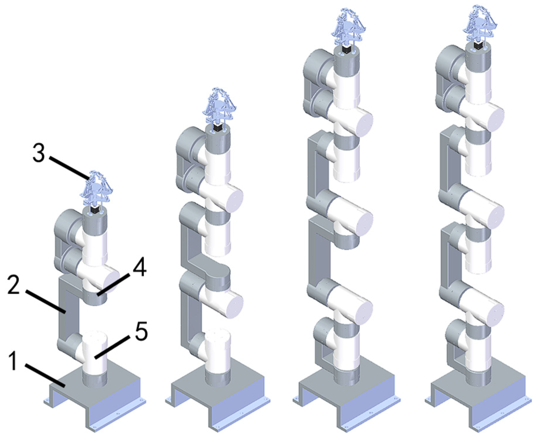
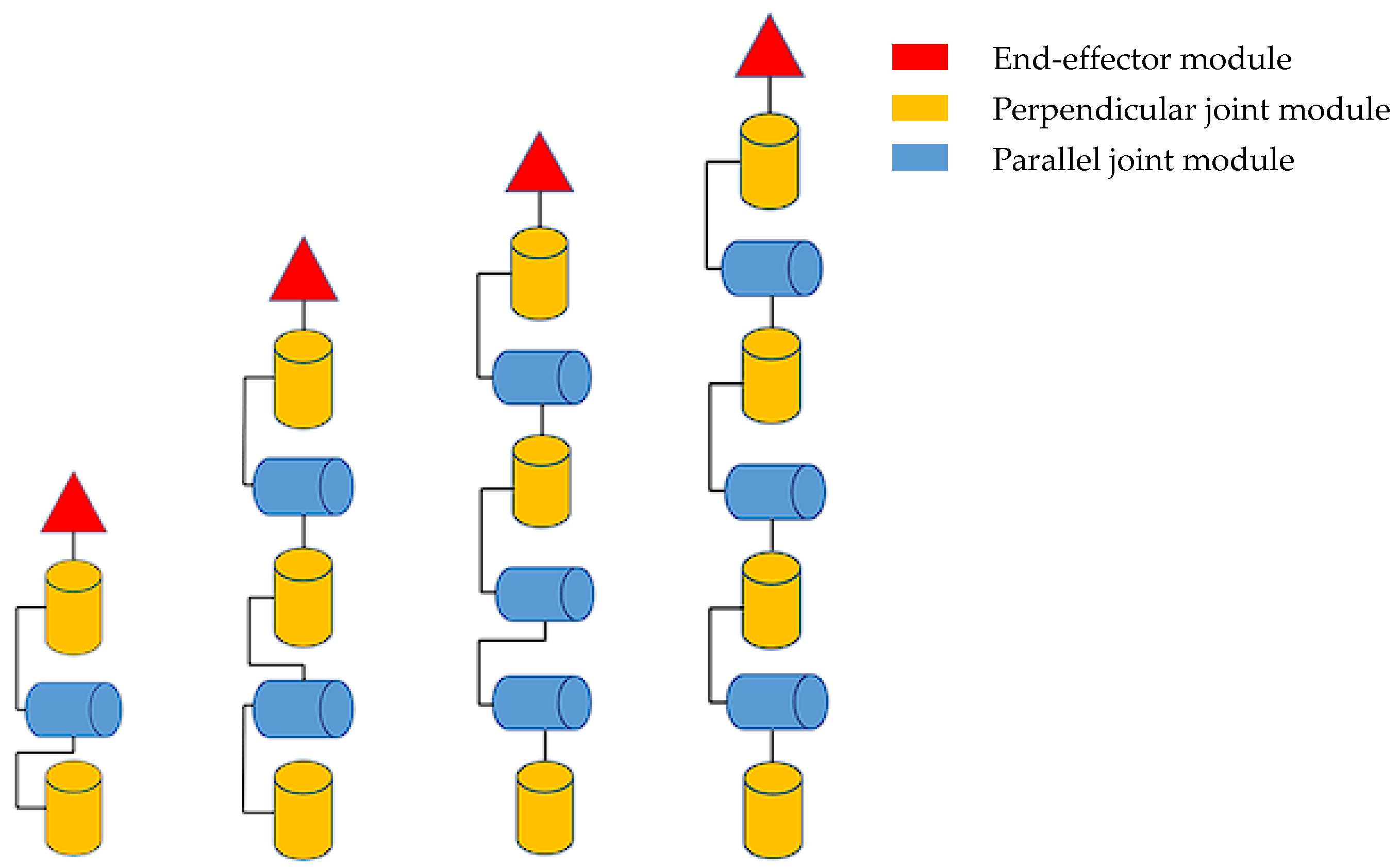
• All the components of the manipulator are modularized, allowing the assembly of various configurations with different degrees of freedom using existing modular joints, linkages, and end-effectors to meet diverse task requirements;
• The joint module features a highly integrated design, incorporating motors, brakes, reducers, and encoders within the joint. This ensures full functionality while achieving a compact and lightweight structure;
• The modular docking mechanism is designed to connect each module, including its fixation to the base, through a specially designed docking interface. This enhances the assembly and disassembly efficiency while facilitating the maintenance and upkeep of the manipulator;
• The integrated wireless energy transfer module is designed to be embedded in the docking mechanism, enabling plug-and-play functionality for each module and eliminating the need for electrical interface design. Additionally, each module features a hollow routing structure to prevent wire entanglement and related issues during manipulator operation;

The design requirements for each target parameter of the modular reconfigurable manipulator are specified in

Table 1. Target design parameters.

Technical Indicators	Parameters
Overall quality of the manipulator	≤12 kg
Manipulator span length	≤1.3 m
Acceleration of each joint	${0.6 \mathrm{r}\mathrm{a}\mathrm{d}/\mathrm{s}}^2$
Angular velocity of each joint	0.3 rad/s
Manipulator load	≤1 kg
Degrees of freedom	3–7

.

2.2. Structural Design

To enhance the flexibility and reconfigurability of the modular manipulator, a module library has been established. It consists of one T-shaped joint module, four linkage modules, one docking mechanism module, and one end-effector module. These modules enable the assembly of manipulators with different configurations. The specific parameters of these configurations are listed in

Table 2. Parameters for different configurations.

Degrees of Freedom	Mass Estimation (kg)	Manipulator Length (m)	Number of Connecting Rod Modules
3	5	0.78	2
5	8	1.13	3
6	9	$1.30$	$4$
7	11	1.33	4

. As shown in Figure 1, four manipulator configurations are assembled, with degrees of freedom of 3, 5, 6, and 7 from left to right, allowing them to meet different task requirements.

The specific modules comprising each manipulator configuration are shown in Figure 2. Triangles (red) represent the end-effector modules, while cylinders (blue and yellow) denote the joint modules, which can be positioned either perpendicular or parallel to the base. Thin lines indicate the shapes of the linkage modules and the interface positions where they connect to the corresponding joint modules.

All four manipulator configurations feature a wrist joint where three axes intersect at a single point. This design allows the end-effector to rotate freely in three spatial coordinate directions, enabling flexible grasping from various angles and improving operational efficiency. Additionally, the wrist joint design satisfies Pieper’s criterion, ensuring a closed-form solution for inverse kinematics.

A greater variety of joint modules reduces the number of required linkage modules, while the length of the linkage significantly affects the overall design. Additionally, as the degrees of freedom increase, the assembled manipulator becomes longer, resulting in a reduced structural rigidity and the decreased precision of the joint module operation. Moreover, solving both forward and inverse kinematics becomes more complex. Therefore, this paper focuses on the modular structural design of the manipulator, the establishment of modular kinematics, a workspace analysis, motion trajectory planning, and dynamic simulation experiments.

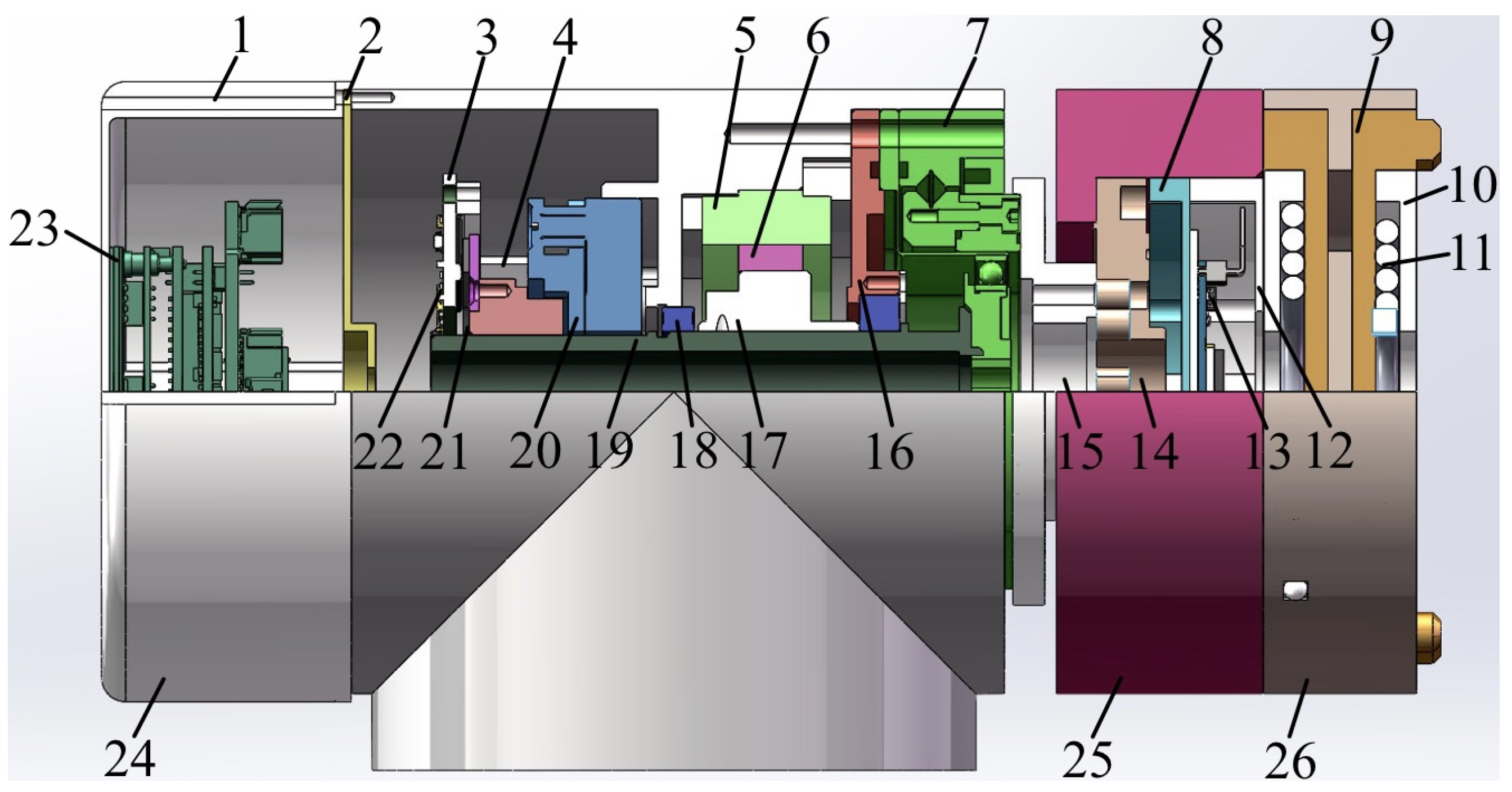
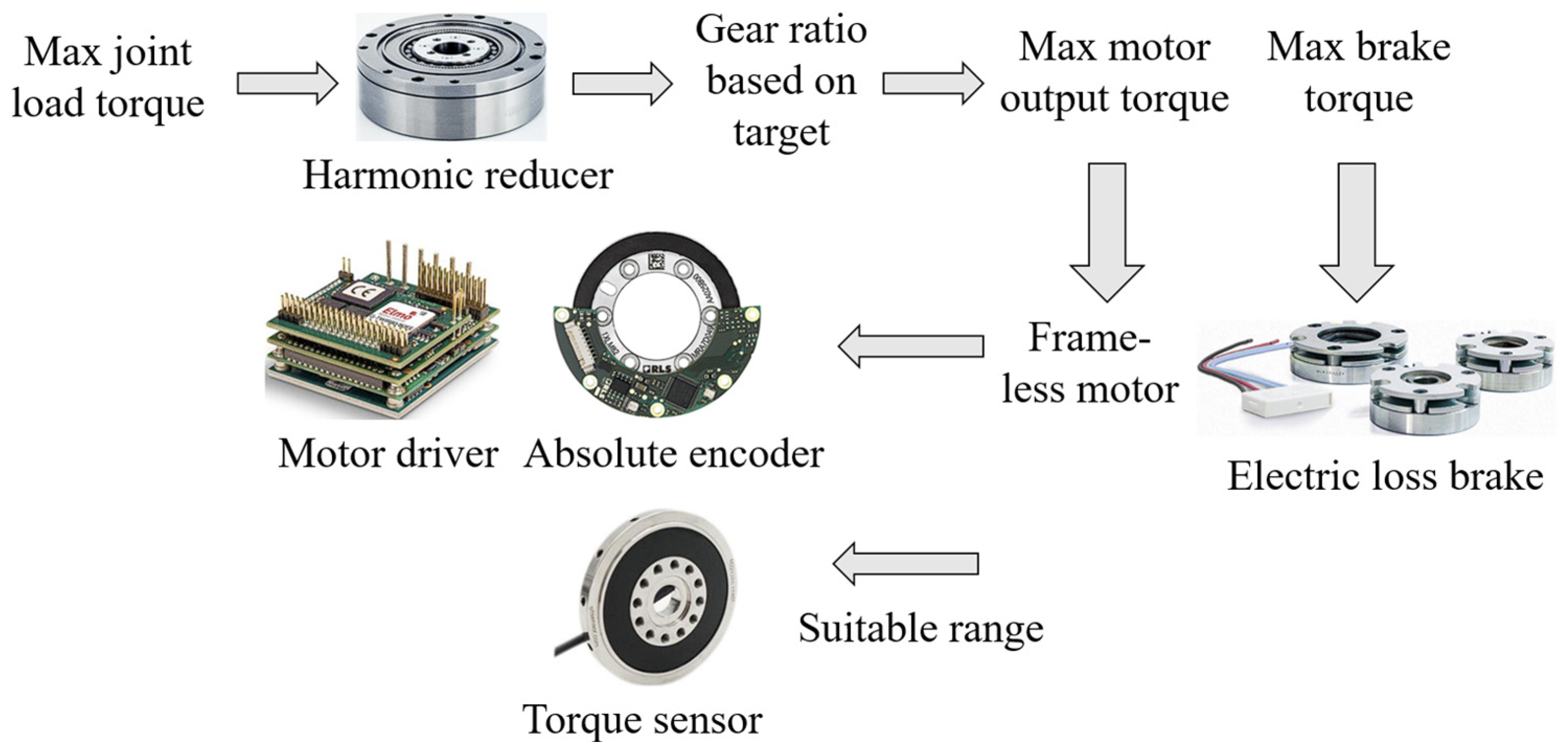
3. Design of Joint Module

3.1. Structural Design of the Joint Module

The designed modular joints are essential not only for driving each output axis of the manipulator but also for rotating the end-effector. These joints are the core components that enable the manipulator to achieve various motion capabilities and functional requirements. Therefore, after selecting the primary components inside the joint module, a specialized design of the internal structure is required to meet the joint module’s key features, such as high integration, compactness, and interchangeability. Additionally, to facilitate efficient assembly, the design should focus on optimizing the assembly sequence and methods for the components within the joint module, ensuring rapid assembly.

The internal structural cross-section of the joint module in this design is shown in Figure 3. While meeting the functional requirements of the joint module, the design also focuses on optimizing the structure to be as compact and lightweight as possible.

3.2. Force Analysis

Taking the designed 6-degree-of-freedom manipulator as an example, the forces and moments during its actual operation are analyzed, in conjunction with the target design parameters of the manipulator. First, the mass of each joint module, linkage module, and end-effector module is estimated. For simplification, the mass of the linkage module is assumed to be concentrated at the center of mass of the adjacent fixed joints. Based on the internal components and structural dimensions of each module, the mass of the joint module is estimated to be 1.4 kg, and the mass of the end-effector and its load is set at 0.65 kg. Since the friction force on the joint module is minimal during the robot’s operation, it is neglected in the force analysis. From this analysis, it can be concluded that, when frictional forces on the joints are ignored, the worst-case force scenarios for joint modules 1 and 2 occur in the two working states shown in Figure 4. In these states, the forces on each joint module are the most critical during operation. Here, ${\mathrm{m}}_{\mathrm{i}}$ represents the mass of each module, and $L_{\mathrm{i}}$ denotes the distance between the geometric centers of the two modules marked in the figure.

In the first load condition, joint module 1 is subjected only to the gravitational load from joint module 2 to the end-effector.

$$F_1={\displaystyle \sum _{i=2}^7{m}_i\mathrm{g}}$$

(1)

In the second load condition, joint module 2 bears not only the gravitational load from joint module 3 to the end-effector but also the inertial load. In this condition, the rotational inertia $J_2$ of joint module 2 is:

$$J_2={\displaystyle \sum _{i=3}^7{m}_i{L}_{i-1}^2}$$

(2)

From the target design parameters, the maximum angular acceleration of each joint is ${\alpha }_{\mathrm{m}\mathrm{a}\mathrm{x}}$ = 0.6 rad/s². Therefore, the inertia load $M_{\mathrm{J}2}$ acting on joint module 2 is:

$$M_{\mathrm{J}2}=J_2{\alpha }_{\max }$$

(3)

The gravitational load $M_{\mathrm{g}2}$ of the joint module 2 is:

$$M_{\mathrm{g}2}={\displaystyle \sum _{i=3}^7{m}_i\mathrm{g}{L}_{i-1}}$$

(4)

Since the weight of each module is an approximation and additional factors (such as friction) have not been considered, a safety factor of K = 1.3 is applied to ensure the reliability of the manipulator design. Among the forces acting on each joint, the maximum force $F_{\mathrm{m}\mathrm{a}\mathrm{x}}$ applied to joint module 1 in the initial state is:

$$F_{\max }=K{F}_1$$

(5)

And among the moments acting on each joint, the maximum load torque $M_{\mathrm{m}\mathrm{a}\mathrm{x}}$ applied to joint module 2 in working condition 2 is:

$$M_{\max }=K\left(M_{J2}+M_{\mathrm{g}2}\right)$$

(6)

From Equations (5) and (6), the appropriate model of the harmonic reducer can be determined. Based on this selection, the reduction ratio is then determined to obtain the maximum output torque required by the motor and the maximum braking torque required by the brake, which serve as the selection criteria for the frameless motor and brake, respectively.

Finally, a torque sensor with an appropriate range is selected according to the design parameters to enhance the precision control of the joint module operation, thereby achieving closed-loop force control for each joint module. Additionally, the selection of the motor driver and encoder should prioritize an ultra-lightweight and compact design. The selection scheme for the key components of the joint module is shown in Figure 5.

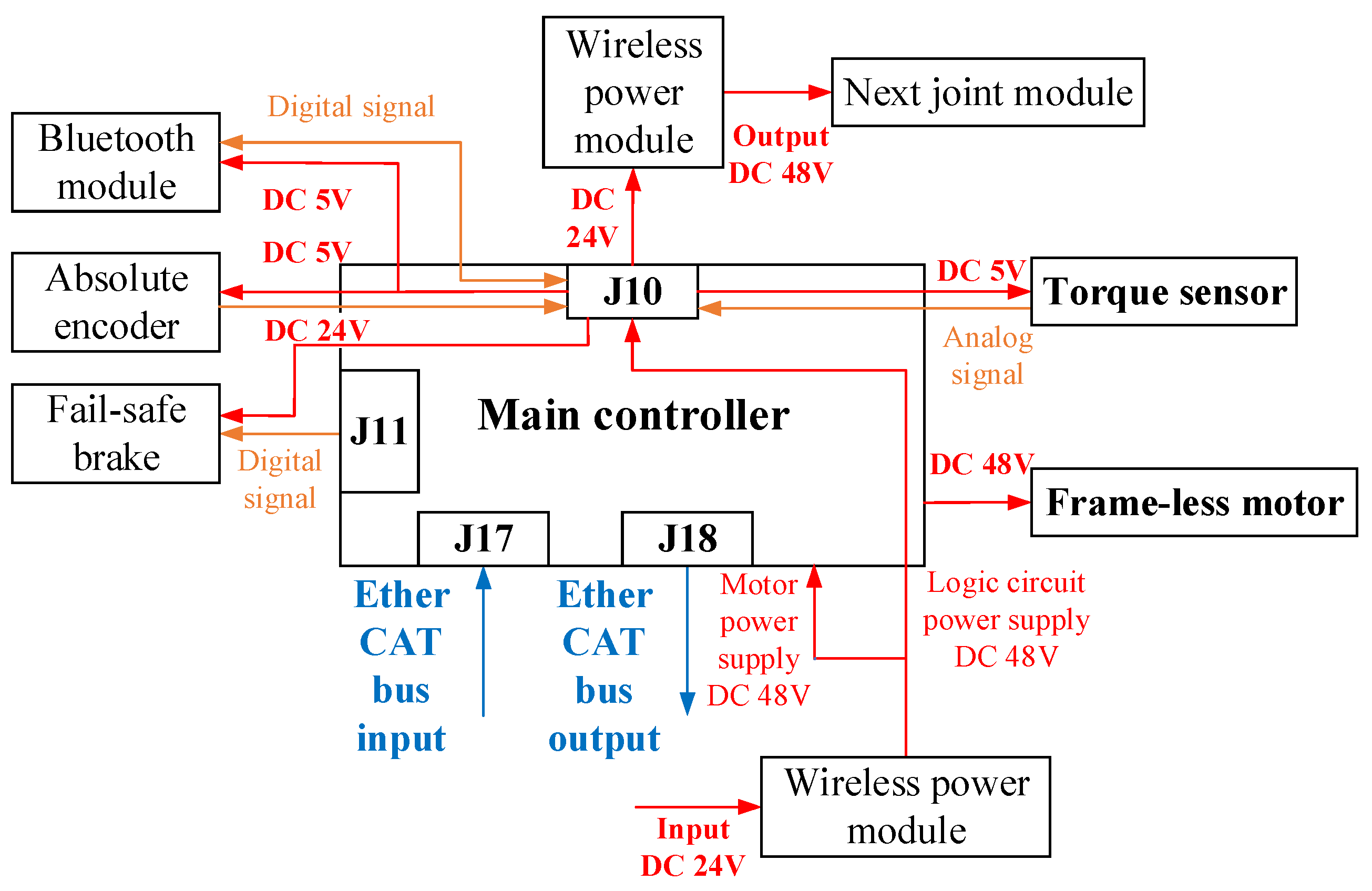
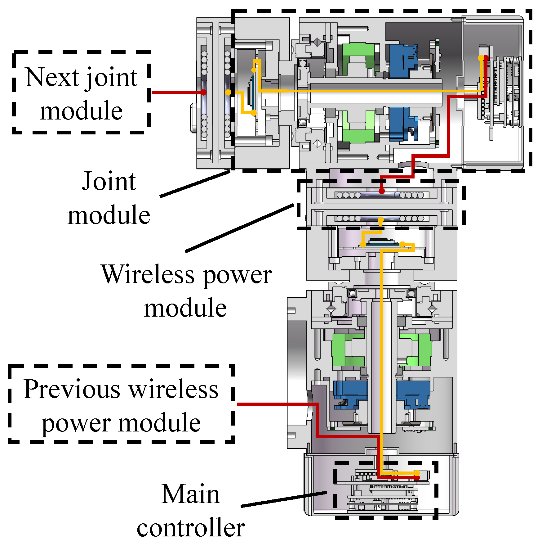
3.3. Electrical Connection and Wiring Layout of the Joint Module

To achieve cable-free connections between modules, a well-structured internal wiring layout is essential. A hollow routing method is adopted for all the modules to prevent cable entanglement and enhance modularity. The linkage module has a relatively simple wiring layout, consisting only of power transmission lines between the wireless energy transfer modules at both ends. The joint module, however, contains the highest number of internal components, making its wiring layout the most complex. Before designing the wiring layout of the joint module, it is crucial to define the electrical and communication connections of its key components. Figure 6 illustrates the actual electrical and communication connections inside the joint module: red lines represent power supply lines; blue lines represent EtherCAT bus lines; and orange lines represent communication lines.

In the proposed communication model between the modules, data transmission over Bluetooth and EtherCAT is divided into two distinct packet types. The first, referred to as the control command packet, includes four primary parameters: the target position, defining the desired location of the manipulator’s end-effector or joints (typically represented in Cartesian coordinates or joint angles); the target speed, specifying the manipulator’s intended velocity; the target acceleration, detailing the planned rate of change of velocity; and the torque/force command, controlling the torque or force applied to the joints or end-effector. The second, termed the sensor data packet, contains essential feedback: position feedback, reporting the actual position of the joints or end-effector (measured by sensors such as encoders or potentiometers); speed feedback, derived from position data or supplied by velocity sensors (e.g., tachogenerators); and torque/force feedback, indicating the torque or force values measured by dedicated force or torque sensors.

After determining the electrical and communication connections inside the joint module, a hollow alignment layout is employed, as shown in Figure 7.

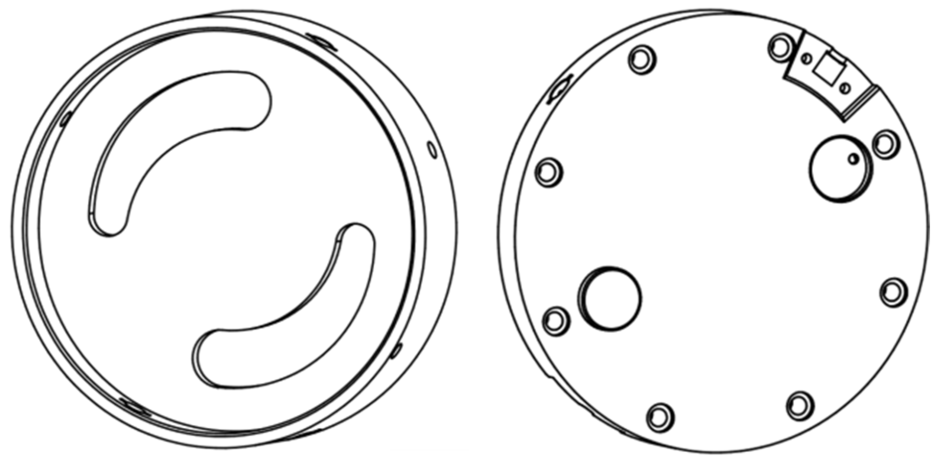
4. Design of the Docking Mechanism Module

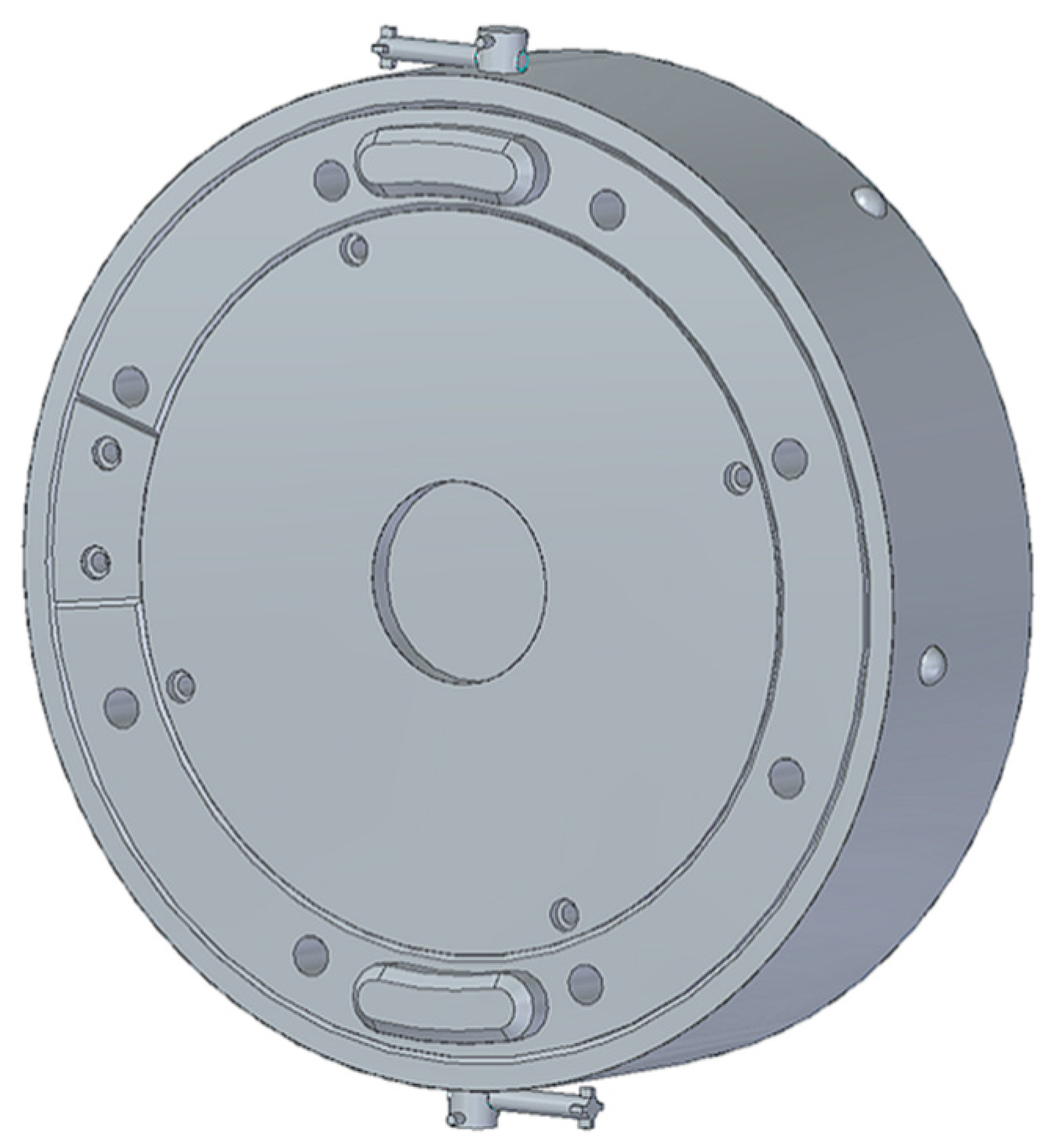
4.1. Structural Design of the Docking Mechanism Module

In existing designs, modules are typically connected using bolts. However, this method proves inconvenient during overall assembly, control software debugging, and the maintenance or replacement of internal parts. To facilitate quick assembly between the modules of a modular reconfigurable manipulator and improve the operational convenience and efficiency, a new docking mechanism module is designed for use at the connection points of joints, linkages, end-effectors, and other modules. The overall assembly model of this docking mechanism module is shown in Figure 8.

The docking mechanism module consists primarily of two fixed heads, one active head, two magnetic coils for wireless energy transfer, four fixed pins, two locking heads, and several springs. The exploded view of the assembly model of this docking mechanism module is shown in Figure 9.

The magnetic coil is placed inside the coil guard and fixed in the central groove of the docking mechanism module’s fixed head. The two fixed heads are bolted to the connection ends of the joint or connecting rod modules, with fixed pins and locking heads designed with limit slots and springs. Figure 10 shows the fixed and active heads of the docking mechanism module. The pre-operation process for the docking mechanism module before completing the docking action is as follows:

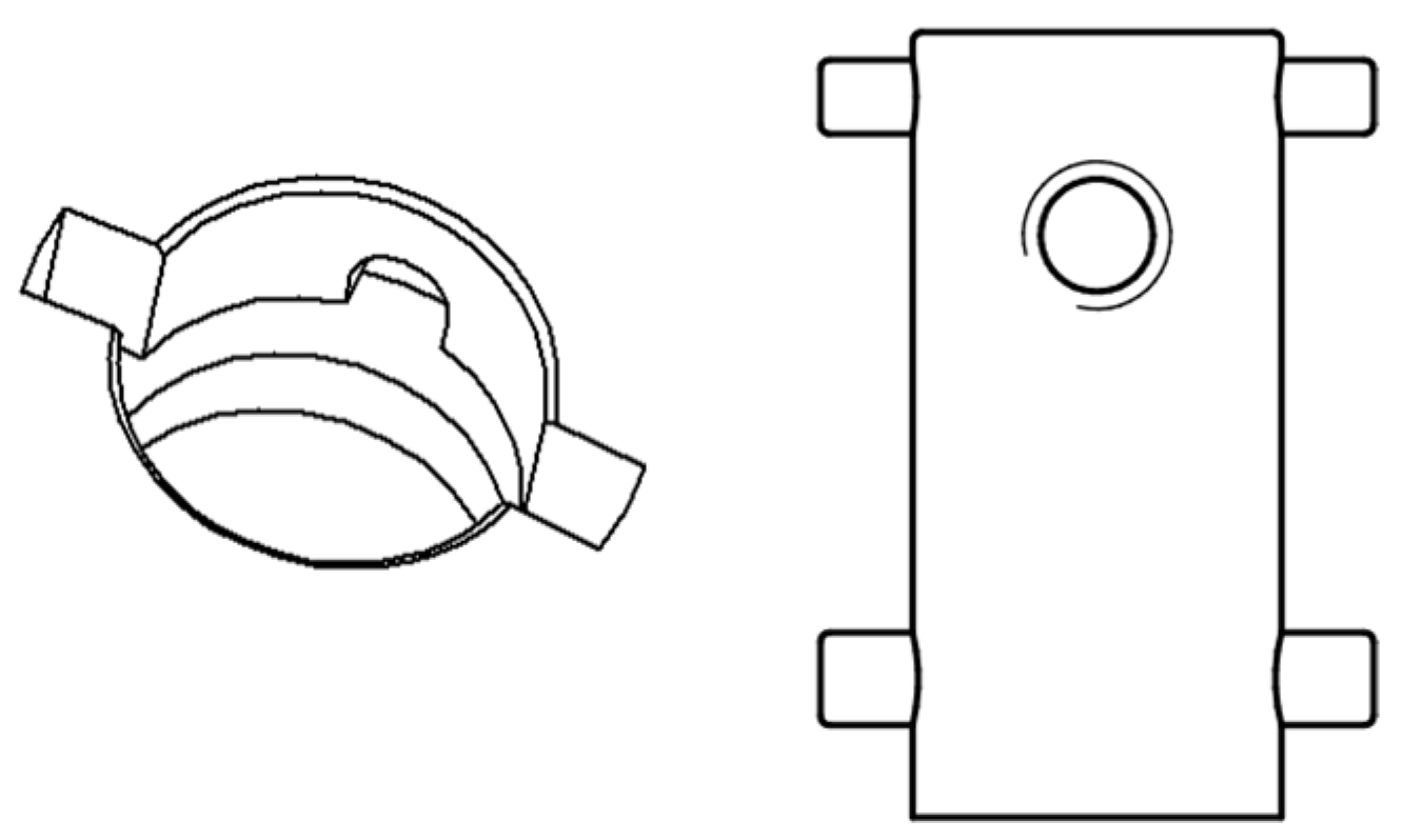
• The magnetic coil for wireless energy transmission is placed inside the coil guard, and the power transmission cable is threaded through the hole in the guard. The cable then connects to the main control board via the hollow drive shaft, enabling power transfer to the next joint module via wireless energy. The coil guard is then bolted to the fixed head of the docking mechanism module.
• The fixed head of the docking mechanism module is first inserted into the correct position via the guiding groove at the connection end, then bolted to the corresponding connection end of each module, preparing the system for the docking operation. If the fixed head is not damaged or the joint module does not require internal maintenance, disassembly is not necessary.
• The spring and spring pin are placed into the spring pin grooves of the fixed head, one set on each side. The bottom of the spring and the spring pin of the locking head are glued to the corresponding end face using an adhesive. When the docking mechanism is not locked, the limit holes of the movable and fixed heads do not overlap. The spring is compressed with a larger deformation, and the spring pin does not push out of the limit holes of the movable head. As a result, the axial and circumferential movements of both heads are not constrained. When the docking mechanism is locked, the limit holes of the movable and fixed heads overlap. Spring compresses with a smaller deformation compared to when the mechanism is unlocked, and the spring pin passes through the limit holes of the movable head to restrain both the fixed and movable heads. A single movable head has two sets of spring pins.

Figure 10. Exploded assembly model of the docking mechanism module.

Figure 10. Exploded assembly model of the docking mechanism module.

This completes the pre-operation for the docking mechanism module before connecting the modules. The docking and separation process of the docking mechanism module to establish connections between modules is as follows:

1.

To connect the modules, the two fixed heads at the connection ends of the modules are inserted into the positioning groove of the other fixed head through the large end of the circular groove on the active head of the docking mechanism module, using the upper tab on the fixed head. At this point, the limit holes of both the active and fixed heads do not overlap, and the spring pins remain in place.

2.

Manually rotate the movable head so that the tab on the fixed head moves from the large end to the small end of the movable head’s circular groove, locking it in place. This creates an axial constraint between the fixed and active movable heads. At this point, the limit holes of both heads overlap, causing the spring pins to eject and constraining the circumferential movement of both heads.

3.

The locking holes of the fixed head and the active head align. The locking head is inserted into the fixed head’s locking hole via the guiding groove on the active head and rotated 90°. Due to the spring’s force, the locking head is pushed upwards. The outwardly protruding cylinders on either side of the locking head’s front end are pushed into the locking slot. Next, manually lift the locking head until its lower end cylinder tightly fits in the locking slot. Then, using a simple hand screw or a knurled bolt, screw it into the locking head’s upper limit through-hole to secure the locking head axially. This prevents the locking head from being compressed by external force and exiting the locking slot. This completes the docking mechanism module’s connection process. The locking holes on the main dynamic head and fixed head, as well as the locking head assembly section, are shown in Figure 11 and Figure 12.

If the spring pin is used alone as the locking mechanism in the docking module, external factors may cause variations in the spring’s compression deformation, leading to undesirable shaking in the docking mechanism. When the spring pin is ejected from the limit hole, using the hand screw bolt to fix the active and fixed heads will cause an uneven tightening force. This can result in one side being tightened more than the other, leading to a misalignment of the spring pin, an uneven force distribution, and difficulty in tightening the bolt on the opposite side. To address this, the locking head is designed to provide additional constraints, reducing radial offset between the active and fixed heads during locking, thereby improving docking reliability. Each fixed head is equipped with two locking heads, and the docking module features two sets of 180°-symmetrical locking heads. Generally, one set is used for locking, but if one set is damaged, the other can be used as a replacement.

4.

To separate the docking mechanism module, first loosen the hand-screwed bolt, rotate the locking head by 90°, and remove it. Then, simultaneously press the spring pin and rotate the movable head, so that the tab on the fixed head moves from the small end to the large end of the movable head’s circular groove. This will separate the modules connected by the two fixed heads, completing the separation of the docking mechanism module.

4.2. Calibration of the Docking Mechanism Module

1.

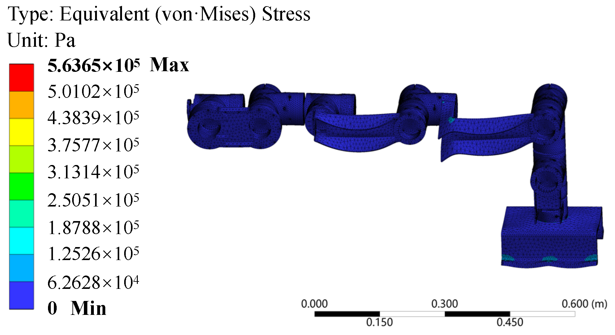
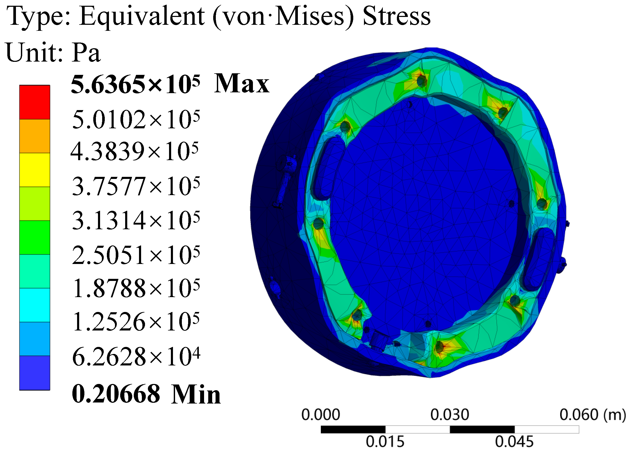
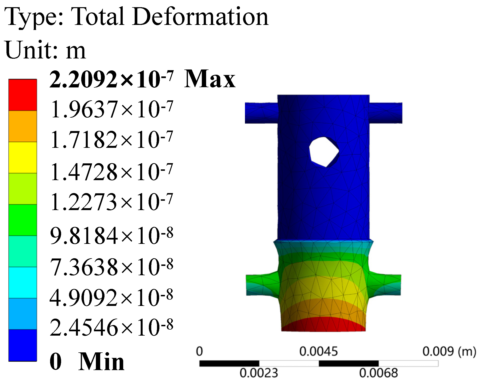
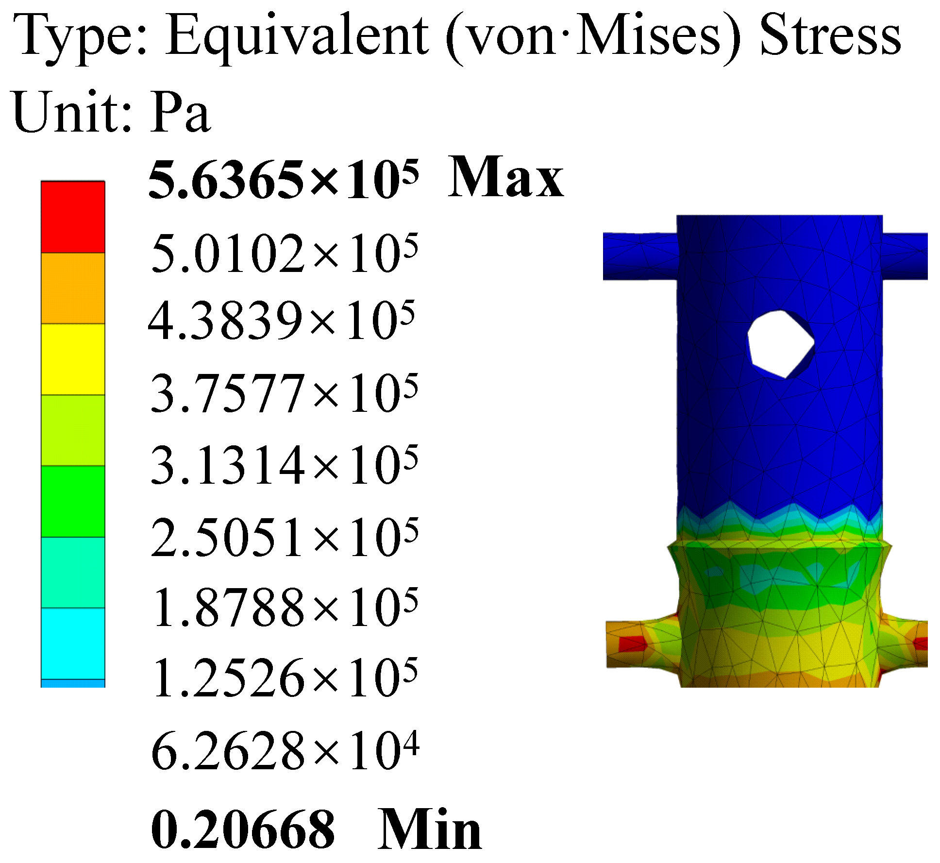
After completing the structural design and force analysis of each module, the deformation and stress are compared against the allowable strength and stiffness values of the selected materials, optimizing and improving any unreasonable structures. Therefore, a finite element analysis must be performed based on the maximum torque calculated from the design parameters, with corresponding external loads and constraints applied. Relevant stress-strain diagrams are generated to analyze the deformation and force state, completing the static analysis and calculation of the entire manipulator and docking mechanism module Define the material properties of each major component.

The materials for the modular joint shell, drive shaft, adapter, locking head, and other components are specified as 7075 aluminum alloy, with an elastic modulus (EX) of 71,000 MPa and a Poisson’s ratio (PRXY) of 0.33. Since the docking mechanism module contains a magnetic coil for wireless energy transmission, high-strength, non-magnetic materials that do not interfere with the magnetic field are required, such as PEEK-CA30 polyether ether ketone (PEEK) engineering plastic. Therefore, the active and fixed heads of the docking mechanism module are made from PEEK-CA30 polyether ether ketone (PEEK) engineering plastic, with an elastic modulus (EX) of 9650 MPa and a Poisson’s ratio (PRXY) of 0.33.

2.

Apply external loads and constraints to them respectively

The connection between each module is achieved via the docking mechanism module, with universal interfaces designed at the connection ends. Power is transmitted through the drive shaft, which also serves as the output shaft for the harmonic reducer [15], while the output end of the end joint bears the load. Based on the previous analysis of the forces and moments under extreme working conditions, gravity-induced acceleration is applied to each component. The maximum load on the output end of the end joint is Fmax = 6.37 N. The bolted connection of the docking mechanism module is modeled as a beam unit, and the bolt preload for the beam unit is set to 4250 N according to the bolt dimensions. Finally, the bolt holes of the base are defined as the fixing constraints.

3.

Model solving and result analysis

After completing the pre-processing steps, each model is solved individually. The post-processing outputs include the deformation of the manipulator, docking mechanism, locking head, and stress distribution, as shown in Figure 13, Figure 14, Figure 15, Figure 16, Figure 17 and Figure 18.

Figure 17 and Figure 18 above show that each connecting rod and docking mechanism module are in a poor stress state. Overall, the stress on the active head and the two fixed heads of the docking mechanism module is relatively uniform, with stress concentration occurring only at the bolt holes. The locking head undergoes overall deformation, with the center of the cylinder concaving towards the stress surface. The deformation increases gradually from the side of the stress surface to the opposite side, with the maximum deformation occurring near the protruding cylinder. The locking head’s middle section, on the left and right sides of the stress surface, experiences uniform stress, with maximum stress located at the top of the vertical surface. The maximum stress in the manipulator occurs at the locking head and the universal connection hole, with a value of 5.63 × ${10}^5$ Pa, and the maximum deformation is 2.21 × 10⁻⁷ m. The locking head is made of 7075 aluminum alloy (permissible stress: 2.515 × 10⁸ Pa) and the docking mechanism module is made of PEEK-CA30 (permissible stress: 1.27 × 10⁸ Pa); therefore, the maximum stress generated (2.515 × 10⁸ Pa) is smaller than the permissible stress of the materials used. Additionally, the maximum deformation is less than 0.001 mm, which will not affect the movement or connection of the manipulator. The strength and stiffness meet the design requirements.

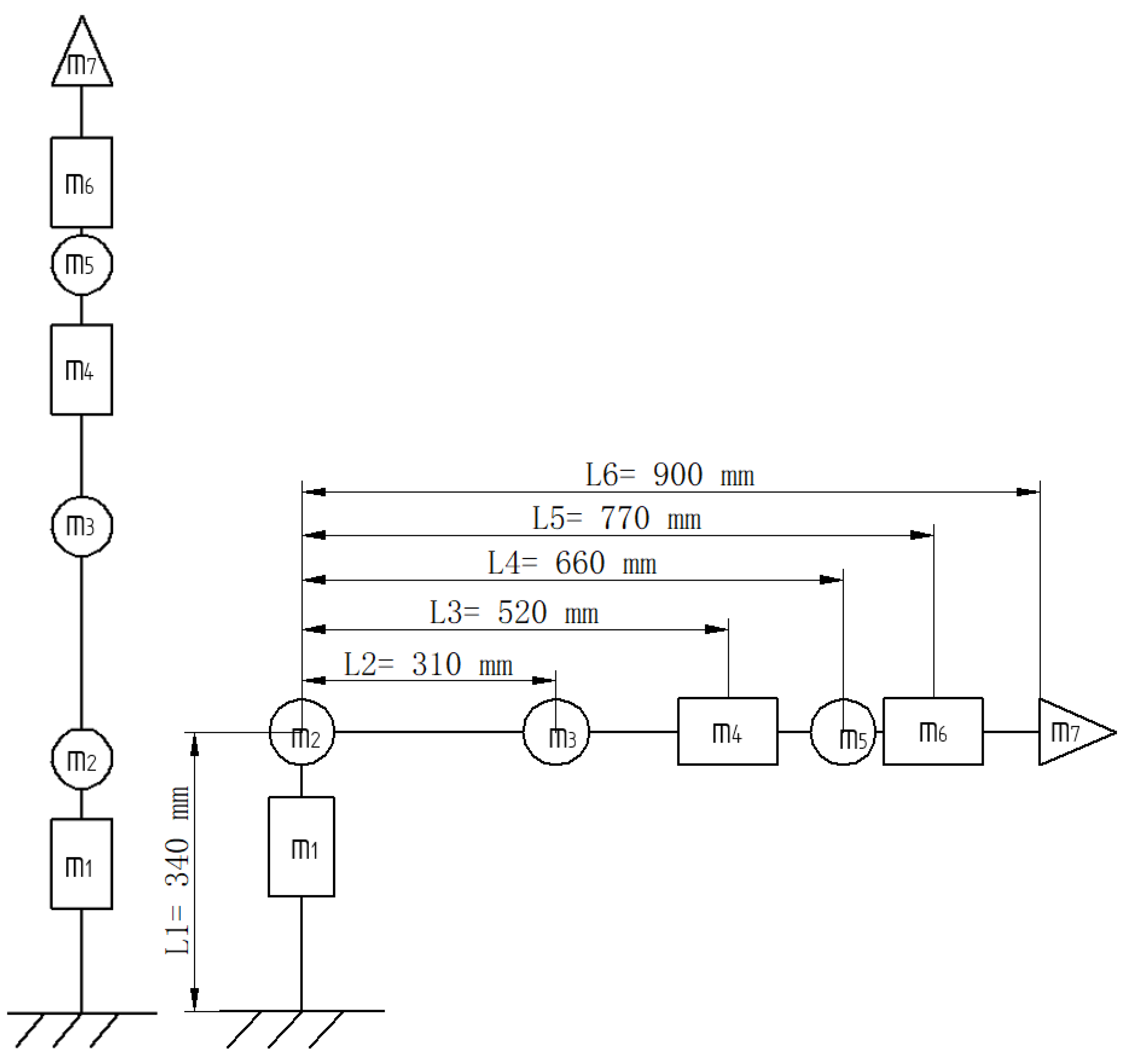
5. Mathematical Modeling and Analysis

5.1. Kinematic Analysis of a Modular Reconfigurable Manipulator

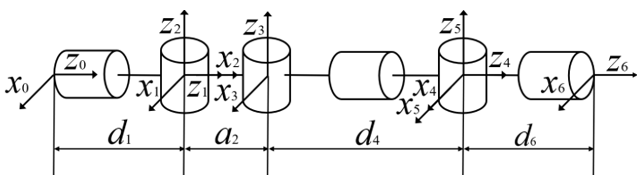
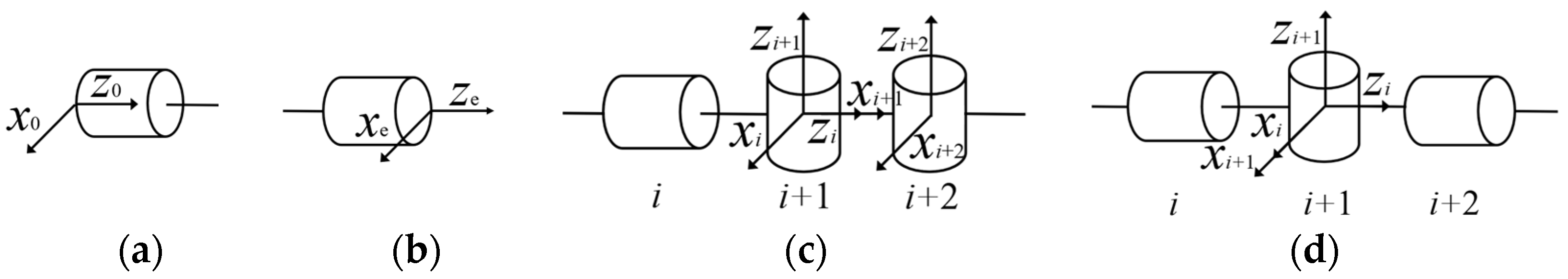
5.1.1. Kinematic Modeling

The improved DH parameter method is used to construct the coordinate system for each joint of the 6-degree-of-freedom modular reconfigurable manipulator and establish the kinematic model. This model describes the positional relationship between the individual links and joints in space. The established kinematic models are shown in Figure 19, and the corresponding DH parameters are provided in

Table 3. DH parameters of a 6-degree-of-freedom modular reconfigurable manipulator.

i	${\mathit{\alpha }}_{\mathit{i}-1}$	${\mathit{a}}_{\mathit{i}-1}$	${\mathit{d}}_{\mathit{i}}$	${\mathit{\theta }}_{\mathit{i}}$
1	0	0	$d_1$	${\theta }_1$
2	${90}^{°}$	0	0	${\theta }_2$
3	0	$a_2$	0	${\theta }_3$
4	$-{90}^{°}$	0	$d_4$	${\theta }_4$
5	${90}^{°}$	0	0	${\theta }_5$
6	$-{90}^{°}$	0	$d_6$	${\theta }_6$

.

The parameters of each connecting rod are defined as follows:

${\alpha }_{i-1}$: The angle by which the z-axis of rod i − 1 is rotated around its x-axis to align with the z-axis of rod i.

$a_{i-1}$: The distance along the x-axis of rod i − 1 by which the z-axis of rod i − 1 is moved to align with the z-axis of rod i.

$d_i$: The distance along the z-axis of rod i by which the x-axis of rod i − 1 is moved to align with the x-axis of rod i.

${\theta }_i$: The angle by which the x-axis of rod i − 1 is rotated around the z-axis of rod i to align with the x-axis of rod i.

5.1.2. Forward Kinematics Solution

The forward kinematics problem involves determining the actual position of the end-effector in space given the rotation angles of each joint. To determine the transformation function of the end link relative to link 0 (the base), the kinematics problem is broken down into n sub-problems involving transformation functions between link i − 1 and link i. Among the four parameters defining a link, only one is variable—the joint angle. Therefore, each sub-problem is further divided into four sub-problems, represented by 4 × 4 transformation matrices ${}_i{}^{i-1}T$.

$$\left\{\begin{array}{l}\cos {\theta }_i=c_i\hfill \\ \begin{array}{c}\cos {\theta }_m\cos {\theta }_n-\sin {\theta }_m\sin {\theta }_n=c_{mn}\\ \sin {\theta }_m\cos {\theta }_n+\cos {\theta }_m\sin {\theta }_n=s_{mn}\end{array}\hfill \end{array}\right.$$

(7)

$${}_{i }{}^{i-1}T=\left[\begin{array}{cccc}{\mathrm{c}}_i& -{\mathrm{s}}_i& 0& a_{i-1}\\ {\mathrm{s}}_i\cos {\alpha }_{i-1}& {\mathrm{c}}_i\cos {\alpha }_{i-1}& -\sin {\alpha }_{i-1}& -d_i\sin {\alpha }_{i-1}\\ {\mathrm{s}}_i\sin {\alpha }_{i-1}& {\mathrm{c}}_i\sin {\alpha }_{i-1}& \cos {\alpha }_{i-1}& d_i\cos {\alpha }_{i-1}\\ 0& 0& 0& 1\end{array}\right]$$

(8)

To enhance the efficiency and convenience of forward kinematic computation for the modular reconfigurable manipulator satisfying the Pieper criterion, a modular kinematic model, illustrated by the coordinate system of each module in Figure 20, is structured into a base module, an end module, and two types of intermediate modules, which are assembled to form the complete manipulator.

The homogeneous transformation matrices of the base and end modules are obtained:

$${}_1{}^{0}T=\left[\begin{array}{cccc}{c}_1& -s_1& 0& 0\\ s_1& c_1& 0& 0\\ 0& 0& 1& d_1\\ 0& 0& 0& 1\end{array}\right]$$

(9)

$${}_{e }{}^{e-1}T=\left[\begin{array}{cccc}{c}_e& -s_e& 0& 0\\ 0& 0& 1& d_e\\ -s_e& -c_e& 0& 0\\ 0& 0& 0& 1\end{array}\right]$$

(10)

When it is intermediate combination 1.

$${}_{i+1}{}^{i }T=\left[\begin{array}{cccc}-s_{i+1}& -c_{i+1}& 0& 0\\ 0& 0& -1& 0\\ c_{i+1}& -s_{i+1}& 0& 0\\ 0& 0& 0& 1\end{array}\right]$$

(11)

$${}_{i+2}{}^{i+1}T=\left[\begin{array}{cccc}{s}_{i+2}& c_{i+2}& 0& a_{i+1}\\ -c_{i+2}& s_{i+2}& 0& 0\\ 0& 0& 1& 0\\ 0& 0& 0& 1\end{array}\right]$$

(12)

When it is intermediate combination 2.

Taking the 6-degree-of-freedom modular reconfigurable manipulator as an example, the homogeneous transformation matrix for each of its links is first calculated according to the above equation as follows:

$${}_1{}^{0}T=\left[\begin{array}{cccc}{c}_1& -s_1& 0& 0\\ s_1& c_1& 0& 0\\ 0& 0& 1& d_1\\ 0& 0& 0& 1\end{array}\right]$$

(13)

$${}_2{}^{1}T=\left[\begin{array}{cccc}-s_2& -c_2& 0& 0\\ 0& 0& -1& 0\\ c_2& -s_2& 0& 0\\ 0& 0& 0& 1\end{array}\right]$$

(14)

$${}_3{}^{2}T=\left[\begin{array}{cccc}{s}_3& c_3& 0& a_2\\ -c_3& s_3& 0& 0\\ 0& 0& 1& 0\\ 0& 0& 0& 1\end{array}\right]$$

(15)

$${}_4{}^{3}T=\left[\begin{array}{cccc}{c}_4& -s_4& 0& 0\\ 0& 0& 1& d_4\\ -s_4& -c_4& 0& 0\\ 0& 0& 0& 1\end{array}\right]$$

(16)

$${}_5{}^{4}T=\left[\begin{array}{cccc}{c}_5& -s_5& 0& 0\\ 0& 0& -1& 0\\ s_5& c_5& 0& 0\\ 0& 0& 0& 1\end{array}\right]$$

(17)

$${}_6{}^{5}T=\left[\begin{array}{cccc}{c}_6& -s_6& 0& 0\\ 0& 0& 1& d_6\\ -s_6& -c_6& 0& 0\\ 0& 0& 0& 1\end{array}\right]$$

(18)

To facilitate the subsequent solution of its inverse kinematics, it is also necessary to derive ${}_3{}^{1}T$, ${}_4{}^{1}T$, ${}_5{}^{1}T$.

$${}_3{}^{1}T={}_2{}^{1}T{}_3{}^{2}T=\left[\begin{array}{cccc}{c}_{23}& -s_{23}& 0& -s_2{a}_2\\ 0& 0& -1& 0\\ s_{23}& c_{23}& 0& c_2{a}_2\\ 0& 0& 0& 1\end{array}\right]$$

(19)

$$\begin{array}{cc}\hfill {}_4{}^{1}T& ={}_3{}^{1}T{}_4{}^{3}T\hfill \\ & =\left[\begin{array}{cccc}{c}_{23}{c}_4& -c_{23}{s}_4& -s_{23}& -s_{23}{d}_4-s_2{a}_2\\ s_4& c_4& 0& 0\\ s_{23}{c}_4& -s_{23}{s}_4& c_{23}& c_{23}{d}_4+c_2{a}_2\\ 0& 0& 0& 1\end{array}\right]\hfill \end{array}$$

(20)

$$\begin{array}{cc}\hfill {}_5{}^{1}T& ={}_4{}^{1}T_5^{4}T\hfill \\ & =\left[\begin{array}{cccc}{c}_{23}{c}_4{c}_5-s_{23}{s}_5& -c_{23}{c}_4{c}_5-s_{23}{c}_5& c_{23}{s}_4& -s_{23}{d}_4-s_2{a}_2\\ s_4{c}_5& -s_4{s}_5& -c_4& 0\\ s_{23}{c}_4{c}_5+c_{23}{s}_5& -s_{23}{c}_4{s}_5+c_{23}{c}_5& s_{23}{s}_4& c_{23}{d}_4+c_2{a}_2\\ 0& 0& 0& 1\end{array}\right]\hfill \end{array}$$

(21)

The matrices are then multiplied sequentially from the right to obtain the transformation matrix ${}_6{}^{0}T$ of the output of the end-effector with respect to link 0 (i.e., the base).

$${}_6{}^{0}T={}_1{}^{0}T_2^1{T}_3^2{T}_4^3{T}_5^4{T}_6^{5}T=\left[\begin{array}{cccc}{n}_x& o_x& a_x& p_x\\ n_y& o_y& a_y& p_y\\ n_z& o_z& a_z& p_z\\ 0& 0& 0& 1\end{array}\right]$$

(22)

An arbitrary set of joint variables (i.e., joint angles) can be given, and the kinematic equations described above can be used to solve for the position and orientation of the end-effector in space with respect to the base reference frame.

5.1.3. Inverse Kinematics Solution

The inverse kinematics solution involves knowing the position and orientation of the end-effector, represented by the transformation matrix ${}_i{}^{i-1}T$, and then solving the joint angles ${\theta }_i$ of each of the other joints.

It is known that when all joints are rotary joints, if any of the following conditions are met—the axes of three adjacent joints are parallel to each other, or the axes of three adjacent joints intersect at a single point—the serial manipulator must have a closed-form solution, known as the Pieper criterion [16]. Therefore, the manipulator configurations designed in this work, based on the principle of modular reconfigurability, all satisfy the Pieper criterion and have closed-form solutions.

According to Equation (22), multiply ${}_1{}^0{T}^{-1}$ on the left and ${}_6{}^5{T}^{-1}$ on the right simultaneously on both sides of the equation.

$${}_1{}^{0}T{}_6{}^{-10}T_6^5{T}^{-1}={}_2{}^{1}T_3^2{T}_4^3{T}_5^4={}_5{}^{1}T$$

(23)

$${}_0{}^{1}T^{-1}=\left[\begin{array}{cccc}{c}_1& s_1& 0& 0\\ -s_1& c_1& 0& 0\\ 0& 0& 1& -d_1\\ 0& 0& 0& 1\end{array}\right]$$

(24)

$${}_6{}^{5}T^{-1}=\left[\begin{array}{cccc}{c}_6& 0& -s_6& 0\\ -s_6& 0& -c_6& 0\\ 0& 1& 0& -d_6\\ 0& 0& 0& 1\end{array}\right]$$

(25)

$$\begin{array}{c}{}_1{}^{0}T{}_6{}^{-10}T_6^5{T}^{-1}=\left[\begin{array}{cccc}n& o& a& p\end{array}\right]\hfill \\ n=\left[\begin{array}{c}{c}_6\left(c_1{n}_x+s_1{n}_y\right)-s_6\left(c_1{o}_x+s_1{o}_y\right)\\ c_6\left(-s_1{n}_x+c_1{n}_y\right)-s_6\left(-s_1{o}_x+c_1{o}_y\right)\\ c_6{n}_z-s_6{o}_z\\ 0\end{array}\right]\hfill \\ o=\left[\begin{array}{c}{c}_1{a}_x+s_1{a}_y\\ -s_1{a}_x+c_1{a}_y\\ a_z\\ 0\end{array}\right]\hfill \end{array}$$

(26)

$$\begin{array}{c}a=\left[\begin{array}{c}-s_6\left(c_1{n}_x+s_1{n}_y\right)-c_6\left(c_1{o}_x+s_1{o}_y\right)\\ -s_6\left(-s_1{n}_x+c_1{n}_y\right)-c_6\left(-s_1{o}_x+c_1{o}_y\right)\\ -s_6{n}_z-c_6{o}_z\\ 0\end{array}\right]\hfill \\ p=\left[\begin{array}{c}-d_6\left(c_1{a}_x+s_1{a}_y\right)+c_1{p}_x+s_1{p}_y\\ -d_6\left(-s_1{a}_x+c_1{a}_y\right)-s_1{p}_x+c_1{p}_y\\ -d_6{a}_z+p_z-d_1\\ 1\end{array}\right]\hfill \end{array}$$

(27)

1.

Solve for θ₁

$$\left(a_x{d}_6-p_x\right)s_1+\left(p_y-a_y{d}_6\right)c_1=0$$

(28)

$$u_i=\tan {\displaystyle \frac{{\theta }_i}{2}} \cos {\theta }_i={\displaystyle \frac{1-u_i^2}{1+u_i^2}} \sin {\theta }_i={\displaystyle \frac{2u_i}{1+u_i^2}}$$

(29)

After substituting the above equation into Equation (28), both sides of the equation are multiplied by $\left(1+u_1^2\right)$.

$$\left(a_y{d}_6-p_y\right)u_1^2+2\left(a_x{d}_6-p_x\right)u_1+p_y-a_y{d}_6=0$$

(30)

$$u_1={\displaystyle \frac{p_x-a_x{d}_6\pm \sqrt{{\left(a_x{d}_6-p_x\right)}^2+{\left(a_y{d}_6-p_y\right)}^2}}{a_y{d}_6-p_y}}$$

(31)

$${\theta }_1=2{\tan }^{-1}{u}_1$$

(32)

It is known that ${\theta }_1$ has two solutions. When $a_{\mathrm{y}}{d}_6-p_{\mathrm{y}}=0$, then the value of $u_1$ becomes infinite, i.e., ${\theta }_1$ = 180°

2.

Solve for θ₂

$$d_6\left(c_1{a}_x+s_1{a}_y\right)-c_1{p}_x-s_1{p}_y=m -d_6{a}_z+p_z-d_1=n$$

(33)

$$\left\{\begin{array}{l}{s}_{23}{d}_4+s_2{a}_2=m\hfill \\ c_{23}{d}_4+c_2{a}_2=n\hfill \end{array}\right.$$

(34)

$$2m{a}_2{s}_2+2n{a}_2{c}_2=m^2+n^2+a_2^2-d_4^2$$

(35)

According to Equation (29),

$$\begin{array}{c}\left(m^2+n^2+a_2^2-d_4^2+2n{a}_2\right)u_2^2-4m{a}_2{u}_2+\\ m^2+n^2+a_2^2-d_4^2-2n{a}_2=0\end{array}$$

(36)

$$u_2={\displaystyle \frac{2m{a}_2\pm \sqrt{4a_2^2\left(m^2+n^2\right)-{\left(m^2+n^2+a_2^2-d_4^2\right)}^2}}{m^2+n^2+a_2^2-d_4^2+2n{a}_2}}$$

(37)

$${\theta }_2=2{\tan }^{-1}{u}_2$$

(38)

It is known that ${\theta }_2$ has two solutions. If $4a_2^2\left(m^2+n^2\right)-{\left(m^2+n^2+a_2^2-d_4^2\right)}^2<0$, $u_2$ will have no solution, i.e., ${\theta }_2$ has no solution. When the conditions $4a_2^2\left(m^2+n^2\right)-{\left(m^2+n^2+a_2^2-d_4^2\right)}^2\ge 0$ and $m^2+n^2+a_2^2-d_4^2+2n{a}_2=0$ are satisfied, the value of $u_2$ becomes infinite, i.e., ${\theta }_2={180}^{°}$.

3.

Solve for θ₃

$$s_{23}={\displaystyle \frac{m-s_2{a}_2}{d_4}}$$

(39)

$${\theta }_3=\arcsin {\displaystyle \frac{m-s_2{a}_2}{d_4}}-{\theta }_2$$

(40)

4.

Solve for θ₅

$$c_1{a}_x+s_1{a}_y=k_1 -s_1{a}_x+c_1{a}_y=k_2$$

(41)

$$\left\{\begin{array}{l}-c_{23}{c}_4{s}_5-s_{23}{c}_5=k_1\hfill \\ -s_4{s}_5=k_2\hfill \end{array}\right.$$

(42)

Multiply both sides of the second term of the system of equations by $c_{23}$, then add the squared terms from both sides of the system.

$$c_5^2+2k_1{s}_{23}{c}_5+c_{23}^2{k}_2^2+k_1^2-c_{23}^2=0$$

(43)

$$c_5=-k_1{s}_{23}\pm \sqrt{c_{23}^2\left(1-k_1^2-k_2^2\right)}$$

(44)

$${\theta }_5=\arccos \left(-k_1{s}_{23}\pm \sqrt{c_{23}^2\left(1-k_1^2-k_2^2\right)}\right)$$

(45)

It can be shown that ${\theta }_5$ has two solutions. But when $1-k_1^2-k_2^2<0$, $c_5$ will have no solution, i.e., ${\theta }_5$ has no solution.

5.

Solve for θ₄

$$s_4=-{\displaystyle \frac{k_2}{s_5}}$$

(46)

$${\theta }_4=\arcsin \left(-{\displaystyle \frac{k_2}{s_5}}\right)$$

(47)

When $s_5=0$, i.e., ${\theta }_5=0^{°}$ or ${180}^{°}$, $s_4$ will have no solution, i.e., ${\theta }_4$ has no solution.

6.

Solve for θ₆

$$-s_1{n}_x+c_1{n}_y=k_3 -s_1{o}_x+c_1{o}_y=k_4$$

(48)

$$c_4=s_6{k}_3+c_6{k}_4$$

(49)

According to Equation (18),

$$\left(c_4+k_4\right)u_6^2-2k_3{u}_6+c_4-k_4=0$$

(50)

$$u_6={\displaystyle \frac{k_3\pm \sqrt{k_3^2+k_4^2-c_4^2}}{c_4+k_4}}$$

(51)

It is known that ${\theta }_6$ has two solutions. If $k_3^2+k_4^2-c_4^2<$ 0, then $u_6$ will have no solution, i.e., ${\theta }_6$ has no solution. When $k_3^2+k_4^2-c_4^2\ge$ 0 and $c_4+k_4=$ 0, then the value of u6 will be infinite, i.e., ${\theta }_6$ = 180°.

In summary, given a set of joint angles, the kinematic inverse solution for the designed 6-degree-of-freedom manipulator can be computed using the following equation to determine each joint angle:

$$\left\{\begin{array}{l}{\theta }_1=2{\tan }^{-1}\hfill \\ \begin{array}{l}\left({\displaystyle \frac{p_x-a_x{d}_6\pm \sqrt{{\left(a_x{d}_6-p_x\right)}^2+{\left(a_y{d}_6-p_y\right)}^2}}{a_y{d}_6-p_y}}\right)\\ {\theta }_2=2{\tan }^{-1}\\ \left({\displaystyle \frac{2m{a}_2\pm \sqrt{4a_2^2\left(m^2+n^2\right)-{\left(m^2+n^2+a_2^2-d_4^2\right)}^2}}{m^2+n^2+a_2^2-d_4^2+2n{a}_2}}\right)\\ {\theta }_3=\arcsin \left({\displaystyle \frac{m-s_2{a}_2}{d_4}}\right)-{\theta }_2\\ {\theta }_4=\arcsin \left(-{\displaystyle \frac{k_2}{s_5}}\right)\\ {\theta }_5=\arccos \left(-k_1{s}_{23}\pm \sqrt{c_{23}^2\left(1-k_1^2-k_2^2\right)}\right)\\ {\theta }_6=2{\tan }^{-1}\left({\displaystyle \frac{k_3\pm \sqrt{k_3^2+k_4^2-c_4^2}}{c_4+k_4}}\right)\end{array}\hfill \end{array}\right.$$

(52)

When solving for inverse kinematics, it is also important to exclude the singular configurations of the joints.

• When $a_{\mathrm{y}}{d}_6-p_{\mathrm{y}}=0,{\theta }_1$ = 180°, ${\theta }_1$ has a unique solution.
• When $4a_2^2\left(m^2+n^2\right)-{\left(m^2+n^2+a_2^2-d_4^2\right)}^2<0,{\theta }_2$ has no solution. When $4a_2^2\left(m^2+n^2\right)-{\left(m^2+n^2+a_2^2-d_4^2\right)}^2\ge 0$ and $m^2+n^2+a_2^2-d_4^2+2n{a}_2=0$, ${\theta }_2$ = 180°, ${\theta }_2$ has a unique solution.
• When $1-k_1^2-k_2^2<0,{\theta }_5$ has no solution.
• When S₅ = 0, i.e., ${\theta }_2$ = 180° or 180°, ${\theta }_4$ has no solution.
• When $k_3^2+k_4^2-c_4^2<0, {\theta }_6$ has no solution. When $k_3^2+k_4^2-c_4^2\ge 0$ and $c_4+k_4=0$, ${\theta }_6$ = 180°, ${\theta }_6$ has a unique solution.

In addition to the above singular position, the final inverse solution of the manipulator can be obtained with a total of 2 × 2 × 2 × 2 = 16 solutions. In practice, when the position of the target end-effector in space is known, the manipulator can select the optimal solution from all the possible inverse solutions based on the specific situation using different trajectory optimization functions.

5.2. Analysis of the Manipulator’s Workspace and Dexterity

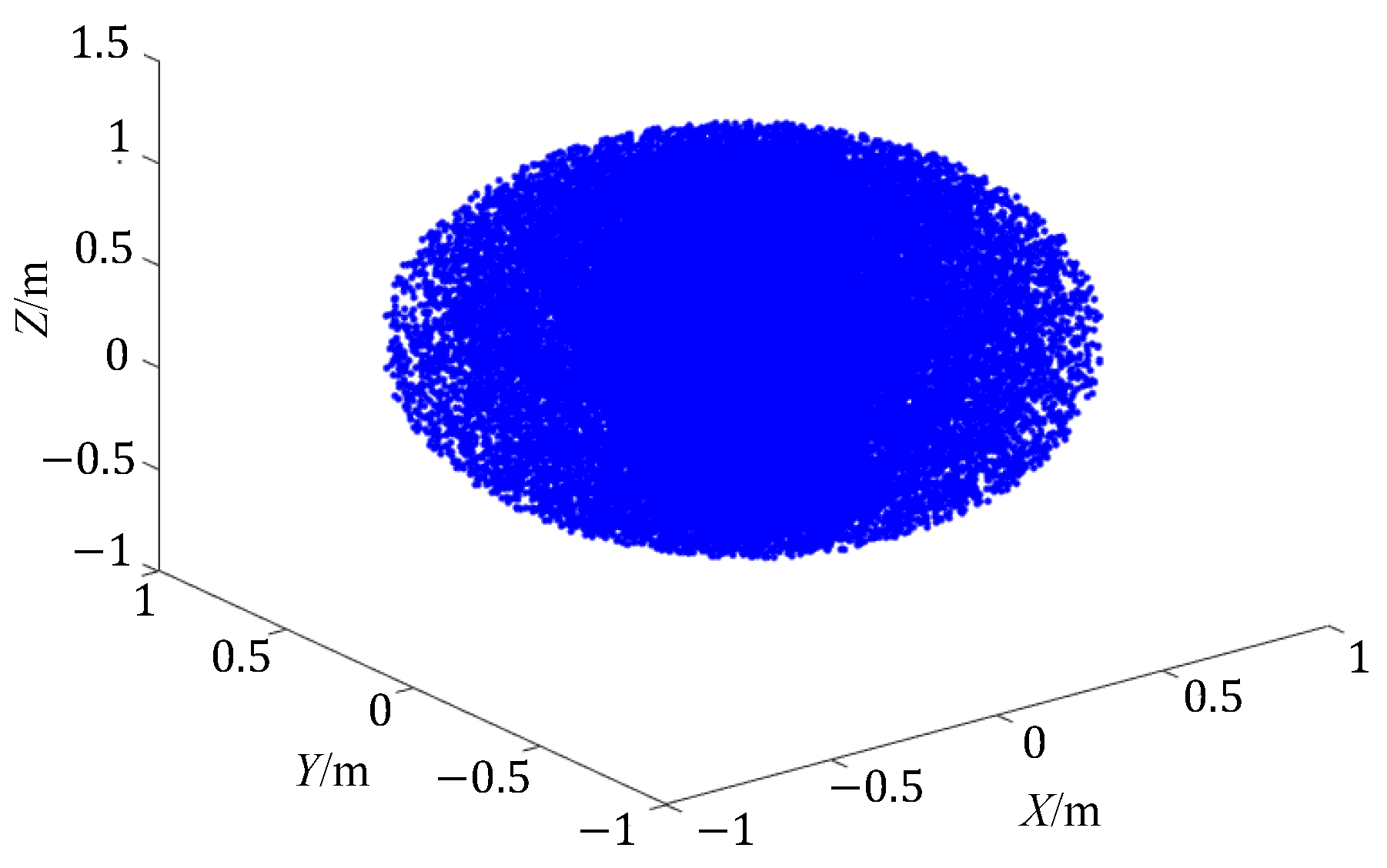
5.2.1. Workspace Analysis

The working space of the manipulator refers to the spatial range that the end-effector can reach. After solving the forward kinematics, the rotational range of each joint is limited by its practical working constraints. Then, each joint performs all the possible movements to determine the positional points of the end-effector in space. When the sampling is sufficiently fine, all the points will form a continuous and closed three-dimensional space, representing the reachable workspace of the manipulator.

Therefore, in this paper, the Monte Carlo method, a typical numerical approach, is used to analyze the workspace of the designed 6-degree-of-freedom modular reconfigurable manipulator.

• A set of joint angles is randomly generated within the specified range, based on the joint angle limits for each joint.
• The generated joint angles undergo kinematic orthogonal computation, and the resulting position of the end-effector is then represented as a point in the Cartesian coordinate system.
• Repeat steps 1 and 2 until the specified number of target sampling points is reached. Finally, plot the resulting set of reachable workspace points, representing the manipulator’s entire workspace.
• The joint angle limits for the designed 6-degree-of-freedom modular reconfigurable manipulator are provided in

  Table 4. Limit range of each joint angle of a 6-degree-of-freedom manipulator.

  Joint	Angle Range
  1	−180°~180°
  2	−150°~150°
  3	−125°~125°
  4	−180°~180°
  5	−100°~100°
  6	−180°~180°

  .

By setting the number of random sampling points to 50,000, a total of 50,000 sets of random joint angles are generated. After numerical computation using the Monte Carlo method, 50,000 end-effector poses are obtained. The resulting workspace of the manipulator in 3D space is shown on Figure 21.

From the above figure, the workspace of the designed 6-degree-of-freedom modular reconfigurable manipulator appears ellipsoidal. The projection in the x-y plane resembles a sphere, while projections in both the y-z and x-z planes resemble ellipsoids. The workspace distribution extends approximately from −0.9 m to 0.9 m in the x-direction, −0.9 m to 0.9 m in the y-direction, and −0.625 m to 1.15 m in the z-direction.

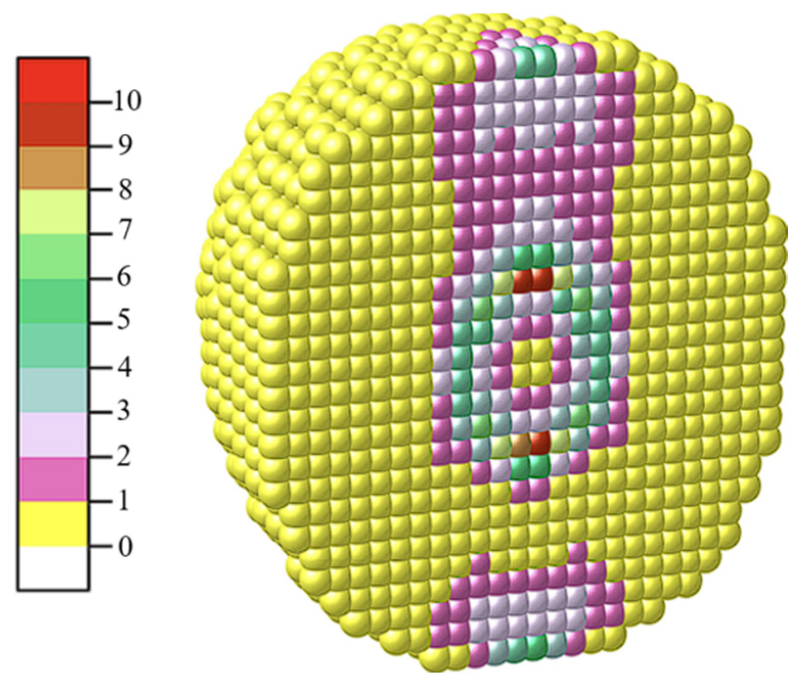
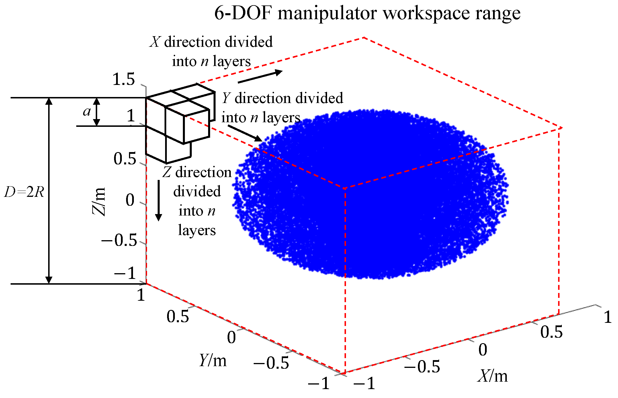
5.2.2. Spatial Dexterity Analysis

Using the Monte Carlo random sampling method described above, the reachable workspace range and the manipulator’s extreme positions in the X, Y, and Z directions can be determined. However, this approach does not provide insight into the dexterous workspace, which represents the manipulator’s operational dexterity [17,18]. This paper focuses on analyzing the dexterity of the workspace of the designed 6-degree-of-freedom modular reconfigurable manipulator using the following steps:

• The obtained workspace is divided into subspaces of equal volume. For the manipulator workspace determined using the Monte Carlo method, a cube is used to fully enclose the workspace, which is then further subdivided into smaller subspaces.

As shown in Figure 22, the working space of the 6-degree-of-freedom manipulator is divided into subspaces. To improve the accuracy and ensure a higher number of sample points in each subspace, 640,000,000 random Monte Carlo sampling points are used. The enveloping cube has a side length D = 2R, where the maximum reach of the modular reconfigurable manipulator, including the end-effector, is 1.3 m. A margin is included to account for unused space. The designed modular reconfigurable manipulator, with a maximum reach of 1.3 m, requires an envelope cube with a margin to fully encompass its workspace. In this case, R is set to 1.35 m, resulting in a cube side length D = 2.7 m. The geometric center of the cube aligns with the base coordinate origin of the manipulator. In this design, the workspace is divided into cubic subspaces of equal volume within the Cartesian coordinate system. The geometric center of each cube is chosen as the subspace center, and the space is divided into n × n × n equal subspaces along the X, Y, and Z axes. Smaller subspaces and a higher number of divisions result in a more accurate density distribution. Therefore, this design uses n = 40, yielding a total of 64,000 cubic subspaces.

The direction of dividing the subspace $X_i{Y}_j{Z}_k($i = 1, 2, 3……n, j = 1, 2, 3……n, k = 1, 2, 3……n) is from the negative direction minimum value of each coordinate axis to the maximum value of the positive direction of each coordinate axis. Subdivision proceeds from the negative minimum to the positive maximum of each axis, following the order Z, Y, and X. In other words, the division starts with 40 subspaces along $X_1{Y}_1{Z}_{\mathrm{k}}$, then moves on to 1600 subspaces along $X_1{Y}_j{Z}_k$, and finally ends with 64,000 subspaces along $X_i{Y}_j{Z}_k$, with each subspace ($X_{init}{Y}_{init}{Z}_{init}$) assigned a unique label.

$$\left(x_{init},y_{init},z_{init}\right)=\left(-R+{\displaystyle \frac{a}{2}},-R+{\displaystyle \frac{a}{2}},-R+{\displaystyle \frac{a}{2}}\right)$$

(53)

The subspace $X_i{Y}_j{Z}_k$ (i = 1, 2, 3……n, j = 1, 2, 3……n, k = 1, 2, 3……n) is defined by the center coordinates $X_i{Y}_j{Z}_k$.

$$\begin{array}{c}\left(x_i,y_j,z_k\right)=\\ \left(x_{init}+\left(i-1\right)a,y_{init}+\left(j-1\right)a,z_{init}+\left(k-1\right)a\right)\end{array}$$

(54)

The dimensions of each subspace along the X, Y, and Z axes are.

$$\begin{gathered} x_iϵ\left[-R+\left(i-1\right)a,-R+ia\right],i=1,2,3\dots \dots n \\ {y}_jϵ\left[-R+\left(j-1\right)a,-R+ja\right],j=1,2,3\dots \dots n \\ {z}_kϵ\left[-R+\left(k-1\right)a,-R+ka\right],k=1,2,3\dots \dots n \end{gathered}$$

(55)

2.

Determine the workspace density of the manipulator. First, find the Cartesian coordinates of each random sample point and identify the corresponding subspace along x, y, z. Next, assign the appropriate subspace label i, j, k, and increment the count of the points in that labeled subspace by one. After counting all the points in each subspace, divide the point count by the volume of the subspace to calculate its density [19]. The calculation follows this equation:

$$a={\displaystyle \frac{D}{n}}$$

(56)

$$v_0=a^3$$

(57)

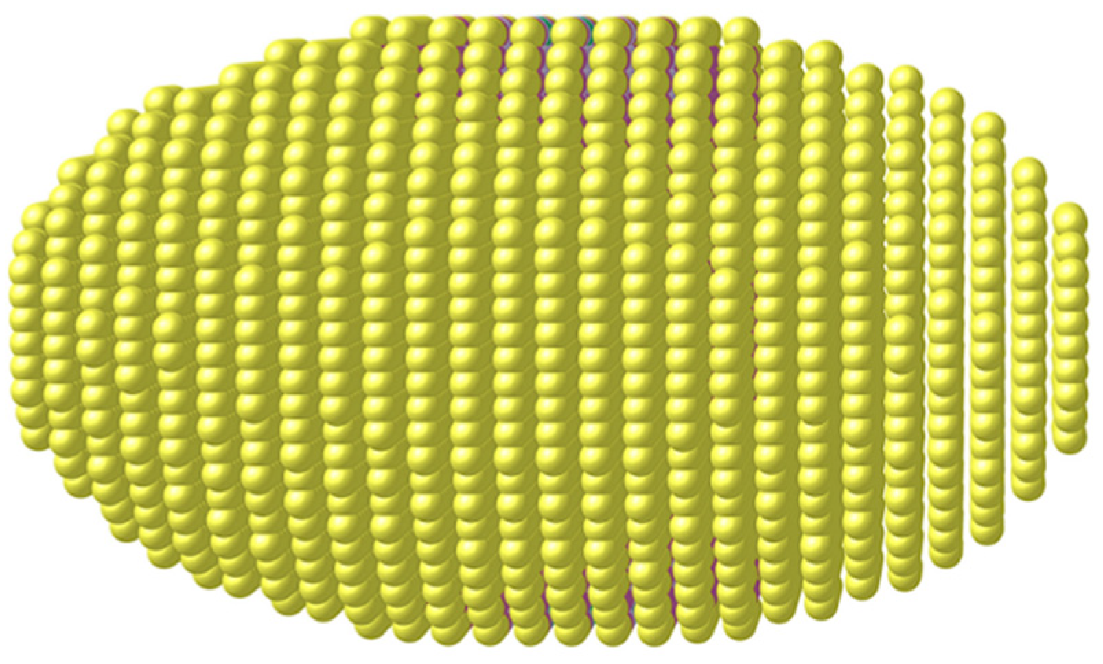
$${\rho }_i={\displaystyle \frac{N_i}{v_0}}$$

(58)

D is the side length of the cube that encloses the manipulator’s workspace;

n is the number of divisions of the manipulator’s workspace along each of the X, Y, and Z axes;

$N_i$ represents the number of random sample points that fall into the i-th subspace based on the end position of the manipulator;

$v_0$ represents the volume of each equally sized small subspace;

a represents the length of each subspace’s side;

${\rho }_i$ represents the workspace density of each subspace;

3.

Classify the workspace density distribution. First, determine the maximum workspace density in each subspace. Then, categorize the density values into intervals using 10% equal divisions, assigning different colors to each range. Finally, generate a visual representation of the manipulator’s workspace density distribution.

As shown in Figure 23, the workspace density distribution of the 6-degree-of-freedom manipulator is represented as spheres of equal volume after importing the center coordinates of each subspace. This visualization facilitates the result analysis. Excluding the subspace corresponding to the inaccessible positions and redundant envelope cubes without random sample points, the overall workspace distribution of the manipulator forms an ellipsoid. This shape aligns with the workspace derived from 50,000 sample points. Increasing the number of random samples further validates the reliability of the obtained workspace distribution along each coordinate axis.

As shown in the workspace density distribution profile of the 6-degree-of-freedom manipulator on Figure 24, the data from each subspace are processed. Half of the data, specifically 32,000 subspaces, are selected. The subspace spheres are classified based on a 10% gradient, corresponding to an isotropic density of 3.130 × 10⁷ ${\mathrm{m}}^{-3}$. Subspace spheres with varying workspace densities are color-coded based on a scale grading. Subspace spheres with varying workspace densities are color-coded based on a scale grading of 3.130 × 10⁸ ${\mathrm{m}}^{-3}$. The next highest density is found in the orange-red sphere region, with values between 2.817 × 10⁸ and 3.130 × 10⁸ ${\mathrm{m}}^{-3}$. The remaining color-coded regions follow the same pattern. Therefore, based on the workspace density distribution graph, the dexterity space of the designed 6-degree-of-freedom manipulator exhibits the following characteristics:

• The gripping workspace distribution of this 6-degree-of-freedom manipulator follows an ellipsoidal shape;
• Starting from the origin of the base coordinate system, the reachable dexterity along the x-axis is greater than along the y-axes and z-axes. This manipulator demonstrates a high dexterity in tasks involving grasping positions and motion trajectories along the x-axis but is slightly less efficient in the y-axis and z-axis directions;
• The trend of dexterity along the x-axis follows a minimum-increasing-maximum-decreasing-increasing pattern, while along the y-axes and z-axes, it follows a minimum-increasing-higher-decreasing-lowest pattern;

Figure 24. 6-DOF manipulator workspace density distribution profile.

Figure 24. 6-DOF manipulator workspace density distribution profile.

5.3. Modular Reconfigurable Manipulator Trajectory Planning and Simulation

The trajectory planning of the manipulator refers to the actual motion path of the end-effector, achieved through the rotation of each joint, as it moves towards the target position to complete the task in the spatial environment [20,21,22].

Generally, there are two main trajectory planning methods for manipulators: joint space planning and Cartesian space planning. This paper uses the designed 6-degree-of-freedom modular reconfigurable manipulator as an example, applying both methods to simulate the motion trajectory and generate the corresponding trajectories and kinematic curves for joint angles, velocities, accelerations, and more.

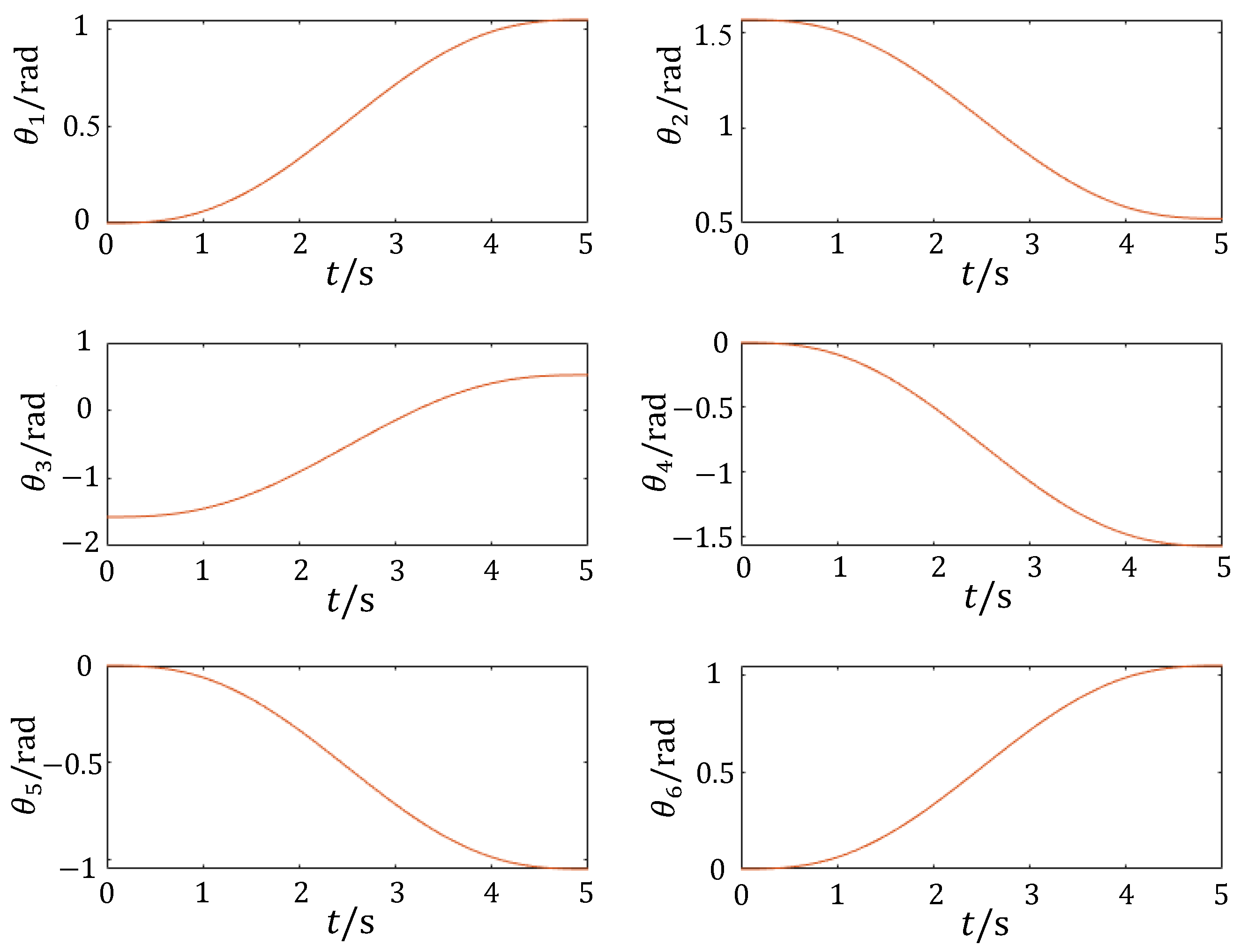
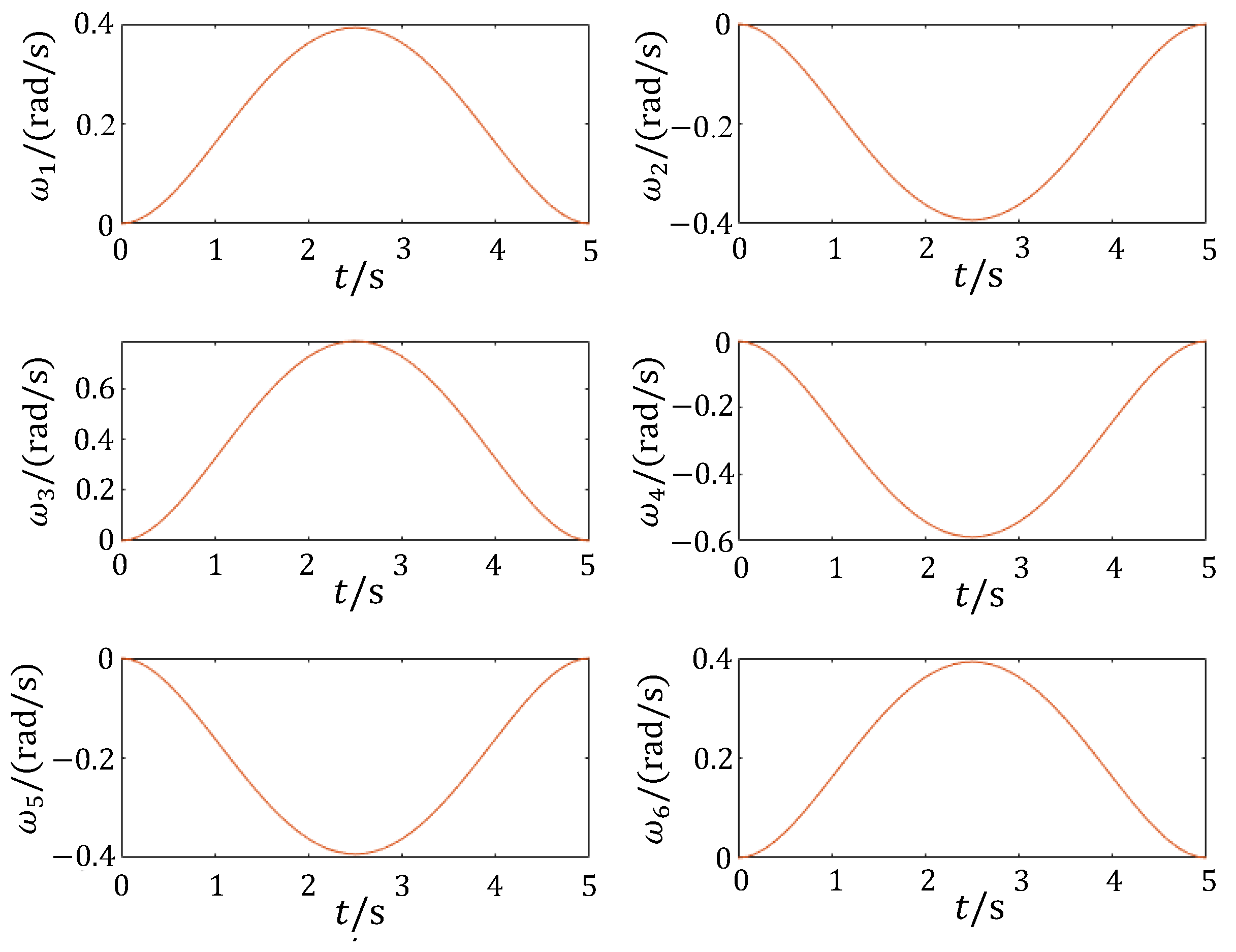
5.3.1. Joint Space Trajectory Planning

The joint space trajectory planning method describes a motion trajectory as a function of the joint angles, with time as the variable. Each path point is determined by the target position of the end-effector relative to the base. The position of each intermediate point is then converted into a set of joint angles using inverse kinematics, allowing a smooth motion curve to be generated by adjusting the number of intermediate points.

Most manipulator trajectory planning methods currently use cubic and quintic polynomial interpolation [23,24]. The position and velocity curves obtained from cubic polynomial interpolation are smooth and continuous. However, the acceleration curves exhibit discrete jumps, making them discontinuous [25]. Due to stricter trajectory requirements, quintic polynomial interpolation is selected for joint space trajectory planning in this design. The specific constraints and solution formulations are as follows.

$$\theta \left(t\right)=a_0+a_{1}t+a_2{t}^2+a_3{t}^3+a_4{t}^4+a_5{t}^5$$

(59)

The quintic polynomial must also satisfy the following constraints.

$$\left\{\begin{array}{l}{\theta }_0=a_0\hfill \\ {\theta }_f=a_0+a_1{t}_f+a_2{t}_f^2+a_3{t}_f^3+a_4{t}_f^4+a_5{t}_f^5\hfill \\ {\dot{\theta }}_0=a_1\hfill \\ {\dot{\theta }}_f=a_1+2a_2{t}_f+3a_3{t}_f^2+4a_4{t}_f^3+5a_5{t}_f^4\hfill \\ {\ddot{\theta }}_0=2a_2\hfill \\ {\ddot{\theta }}_f=2a_2+6a_3{t}_f+12a_4{t}_f^2+20a_5{t}_f^3\hfill \end{array}\right.$$

(60)

$$\left\{\begin{array}{l}{\theta }_0=a_0\hfill \\ {\theta }_f=a_0+a_1{t}_f+a_2{t}_f^2+a_3{t}_f^3+a_4{t}_f^4+a_5{t}_f^5\hfill \\ {\dot{\theta }}_0=a_1\hfill \\ {\dot{\theta }}_f=a_1+2a_2{t}_f+3a_3{t}_f^2+4a_4{t}_f^3+5a_5{t}_f^4\hfill \\ {\ddot{\theta }}_0=2a_2\hfill \\ {\ddot{\theta }}_f=2a_2+6a_3{t}_f+12a_4{t}_f^2+20a_5{t}_f^3\hfill \end{array}\right.$$

(61)

$$\left\{\begin{array}{l}{a}_0={\theta }_0\\ a_1={\dot{\theta }}_0\\ a_2={\displaystyle \frac{{\ddot{\theta }}_0}{2}}\\ a_3={\displaystyle \frac{20{\theta }_f-20{\theta }_0-\left(8{\dot{\theta }}_f+12{\dot{\theta }}_0\right)t_f-\left(3{\ddot{\theta }}_0-{\ddot{\theta }}_f\right)t_f^2}{2t_f^3}}\\ a_4={\displaystyle \frac{30{\theta }_0-30{\theta }_f+\left(14{\dot{\theta }}_f+16{\dot{\theta }}_0\right)t_f+\left(3{\ddot{\theta }}_0-2{\ddot{\theta }}_f\right)t_f^2}{2t_f^4}}\\ a_5={\displaystyle \frac{12{\theta }_f-12{\theta }_0-\left(6{\dot{\theta }}_f+6{\dot{\theta }}_0\right)t_f-\left({\ddot{\theta }}_0-{\ddot{\theta }}_f\right)t_f^2}{2t_f^5}}\end{array}\right.$$

(62)

Based on the above fifth-degree polynomial solution for path planning, the joint space trajectory planning simulation is performed for the designed 6-degree-of-freedom manipulator. First, the parameters of each linkage are used to establish the manipulator model. The initial joint angle is $\left[0, {\displaystyle \frac{\pi }{2}},-{\displaystyle \frac{\pi }{2}}, 0, 0, 0\right]$ and the final joint angle is $\left[{\displaystyle \frac{\pi }{3}}, {\displaystyle \frac{\pi }{6}}, {\displaystyle \frac{\pi }{6}},-{\displaystyle \frac{\pi }{2}},-{\displaystyle \frac{\pi }{3}}, {\displaystyle \frac{\pi }{3}}\right]$. The motion path is divided into 50 intermediate points, with a 0.1-s time interval between each point. The kinematic forward solution is then solved for each set of joint angles, allowing the positions of the intermediate points to be obtained. The corresponding motion trajectory diagrams and the curves of joint angles, angular velocity, and angular acceleration are generated, as shown in Figure 25, Figure 26, Figure 27 and Figure 28.

The generated motion trajectory is shown in Figure 25, illustrating the end-effector’s movement from point A to point B. The curves generated by the joint space trajectory planning method are smooth and continuous, with no discontinuities. The manipulator moves smoothly without path-crossing collisions, indicating that the fifth-degree polynomial interpolation ensures a stable trajectory without a noticeable jitter or sudden jumps. The simulation results confirm that the designed 6-degree-of-freedom modular reconfigurable manipulator meets the kinematic requirements of the target design.

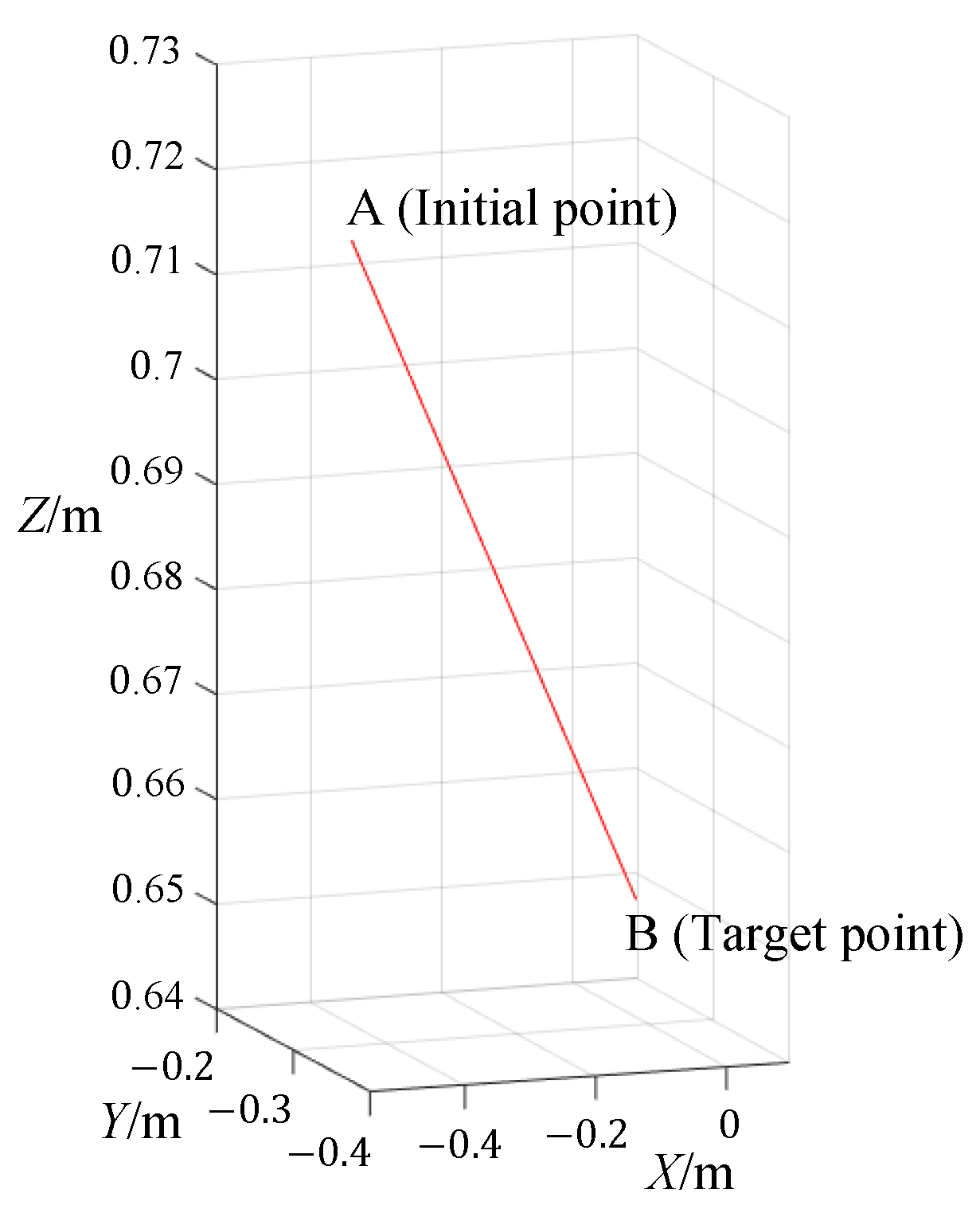
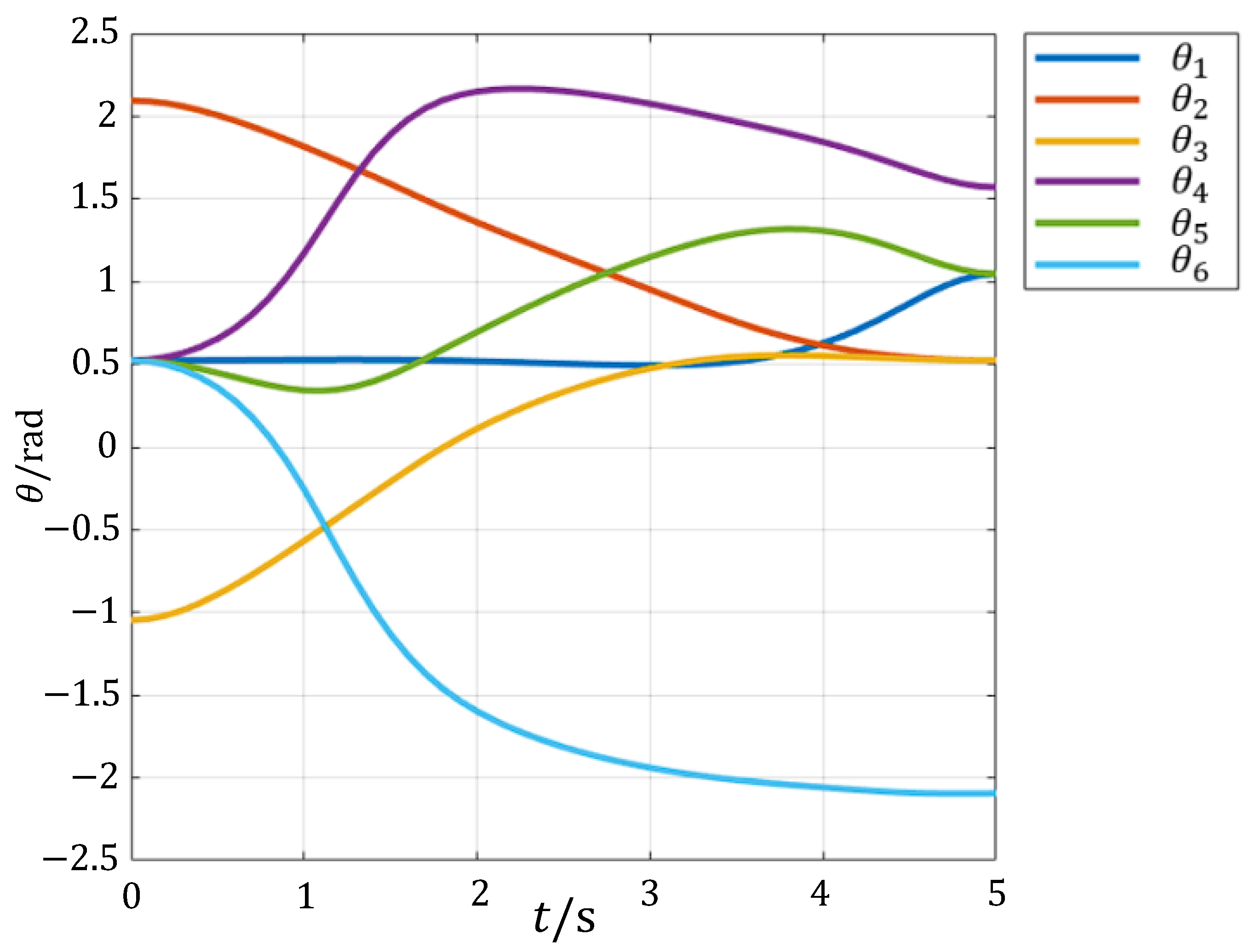
5.3.2. Cartesian Spatial Trajectory Planning

The Cartesian space trajectory planning method describes the motion trajectory as a function of position and orientation in Cartesian coordinates, with time as the variable. Unlike the joint space trajectory planning method, the Cartesian space trajectory planning method must consider issues such as singularities and workspace, as there is a continuous correspondence between the Cartesian motion paths and joint positions [26,27,28]. This paper uses the Cartesian space trajectory planning method with linear interpolation.

The specific steps of the linear interpolation method (with uniform acceleration and deceleration) are outlined below:

• Defining the positions of the start and end points;
• Assume that the velocity v at the output of the end-effector and the time interval between each interpolation is t;
• Calculate the distance L between the start point and end point;

$$L=\sqrt{{\left(x_2-x_1\right)}^2+{\left(y_2-y_1\right)}^2+{\left(z_2-z_1\right)}^2}$$

(63)

4.

Calculate the total interpolation time T;

$$T={\displaystyle \frac{L}{v}}$$

(64)

5.

Calculate the total number of interpolation steps N (rounded);

$$N={\displaystyle \frac{T}{t}}$$

(65)

6.

Calculate the increment for each interpolation step;

$${\Delta }_x={\displaystyle \frac{\left(x_2-x_1\right)}{N}}{\Delta }_y={\displaystyle \frac{\left(y_2-y_1\right)}{N}}{\Delta }_z={\displaystyle \frac{\left(z_2-z_1\right)}{N}}$$

(66)

7.

Based on the increment of each interpolation, the Cartesian coordinates of each point along the line are calculated;

$$x_i=x_1+i{\Delta }_x y_i=y_1+i{\Delta }_y z_i=z_1+i{\Delta }_z$$

(67)

8.

Finally, the position of each interpolation point is substituted into the manipulator’s inverse kinematics for calculation, yielding a set of joint angles to complete the linear interpolation path planning.

The 6-degree-of-freedom manipulator is simulated using the Cartesian spatial trajectory method with linear interpolation. First, the motion trajectory is generated, with the initial and final joint angles set to $\left[0, {\displaystyle \frac{\pi }{2}},-{\displaystyle \frac{\pi }{2}}, 0, 0, 0\right]$ and $\left[{\displaystyle \frac{\pi }{6}}, {\displaystyle \frac{7\pi }{12}},-{\displaystyle \frac{\pi }{3}},-{\displaystyle \frac{\pi }{2}},-{\displaystyle \frac{\pi }{3}}, {\displaystyle \frac{\pi }{3}}\right]$, respectively. The forward kinematics is then used to calculate the corresponding position matrices. Next, 50 intermediate points are placed along the trajectory, with a 0.1 s time interval between them. The inverse kinematics of each position matrix are computed to obtain the joint angles for the intermediate points. Finally, the motion trajectory, along with the joint angles, velocity, and acceleration curves, are shown in Figure 29, Figure 30, Figure 31 and Figure 32.

The linear trajectory generated by this method is shown in Figure 29. From the simulation results, it can be observed that the angular velocity and angle curves generated using the Cartesian trajectory planning method using linear interpolation are smooth and continuous. However, the acceleration curves exhibit jumps, consistent with the uniform acceleration and deceleration model. Despite these acceleration jumps, the overall motion of the manipulator remains smooth, indicating that the trajectory planning process is stable, without noticeable jitter or jumps.

The comprehensive simulation results of both trajectory generation methods show that the Cartesian spatial trajectory planning method involves a much higher computational complexity than the joint space trajectory planning method. Additionally, it must account for singular positions, unreachable points, and other constraints. However, the Cartesian method allows for precise and independent design and control of the end-effector’s path, making it suitable for applications such as manipulator obstacle avoidance and other complex workspaces.

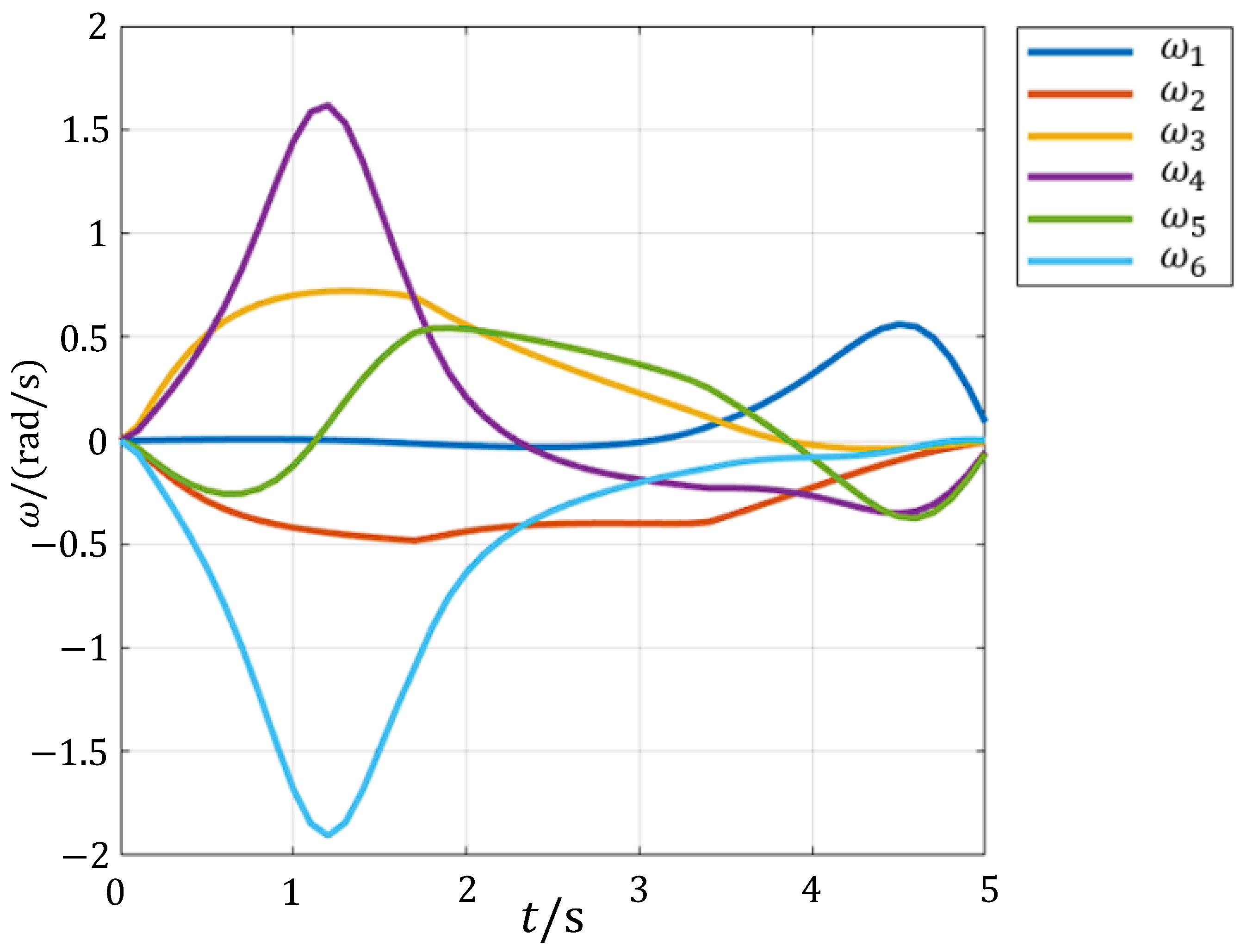
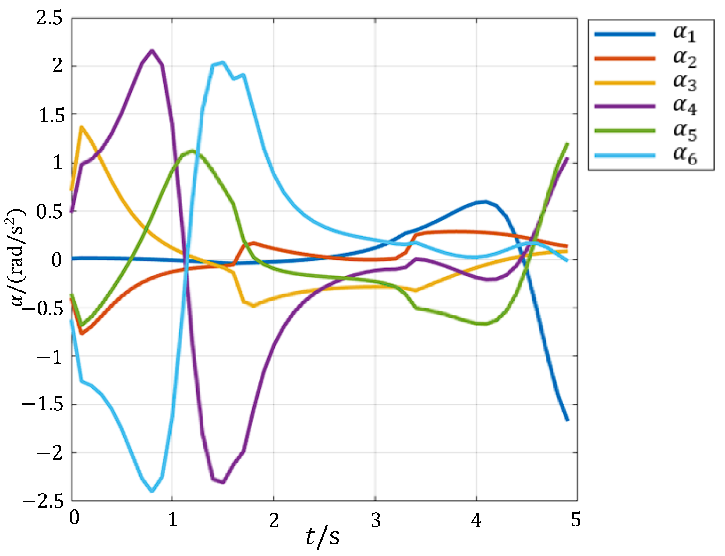
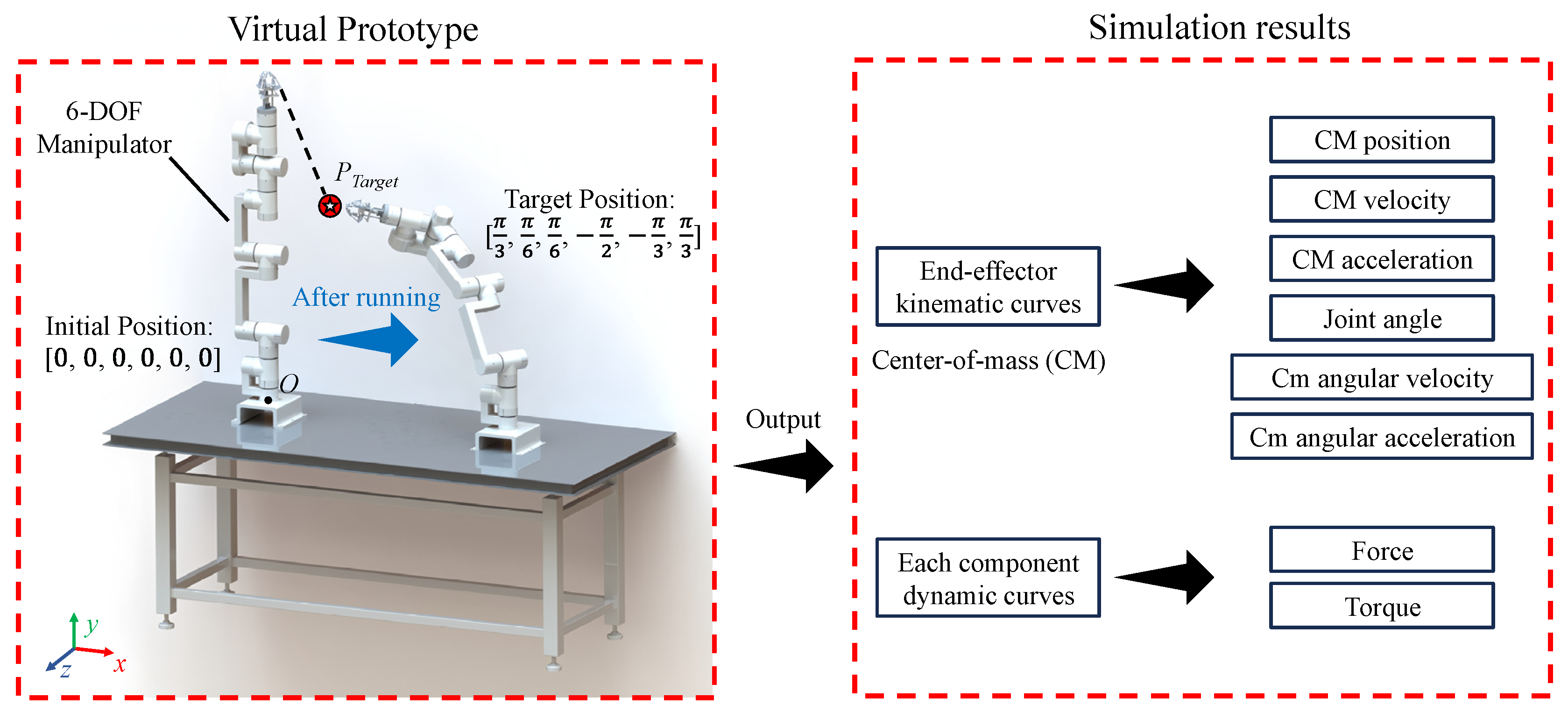
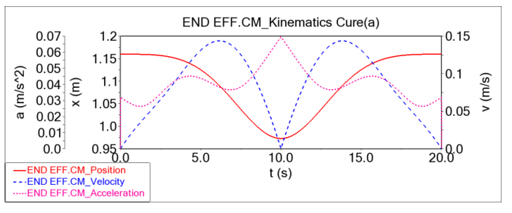
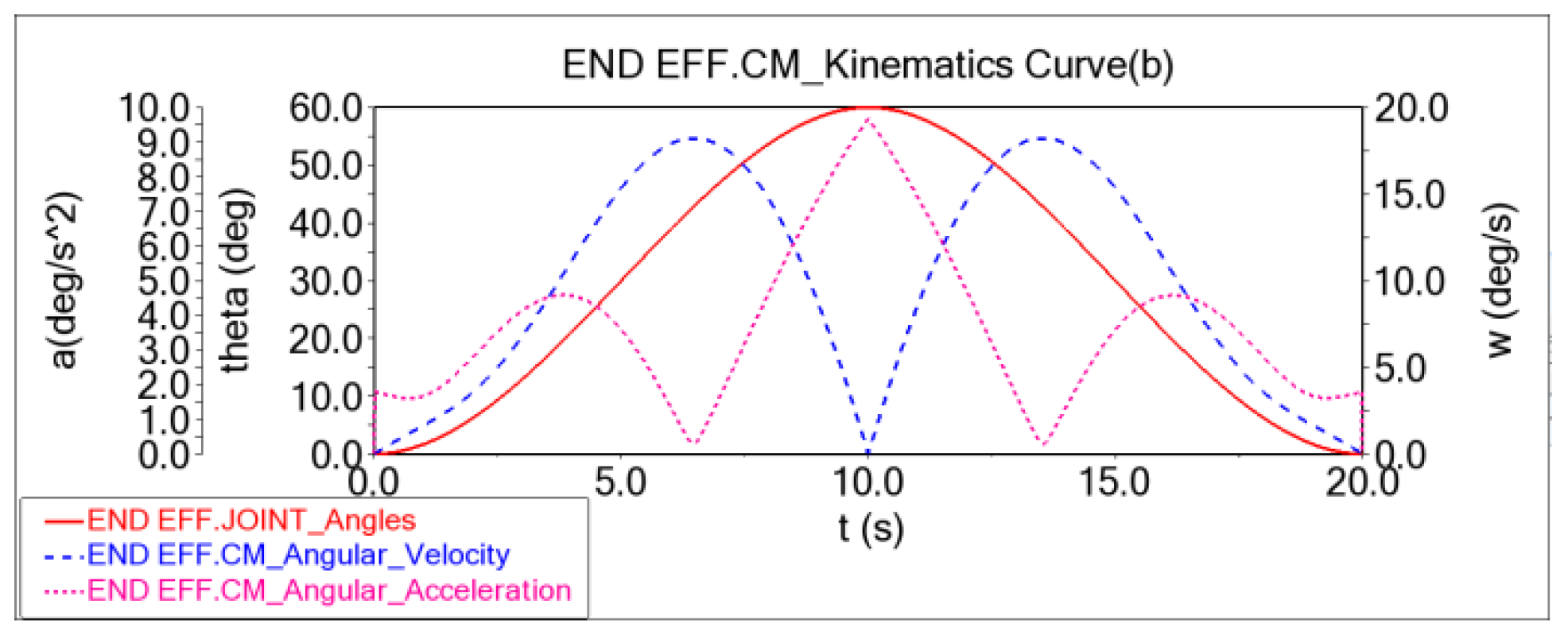
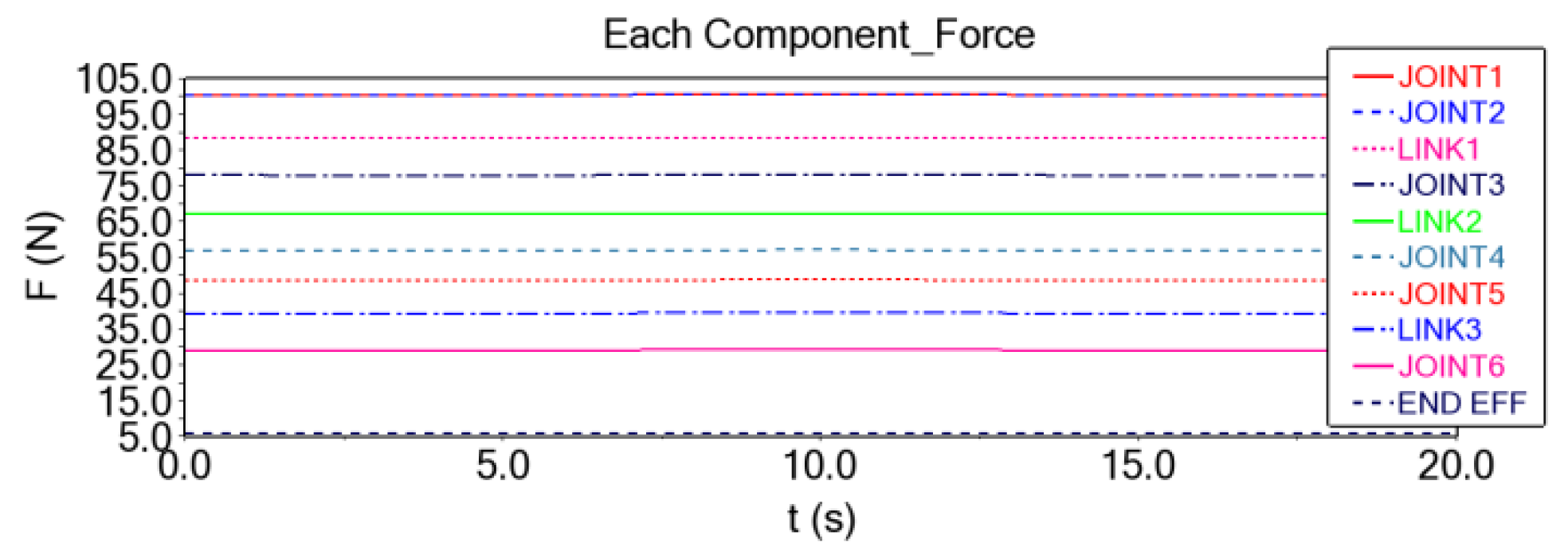
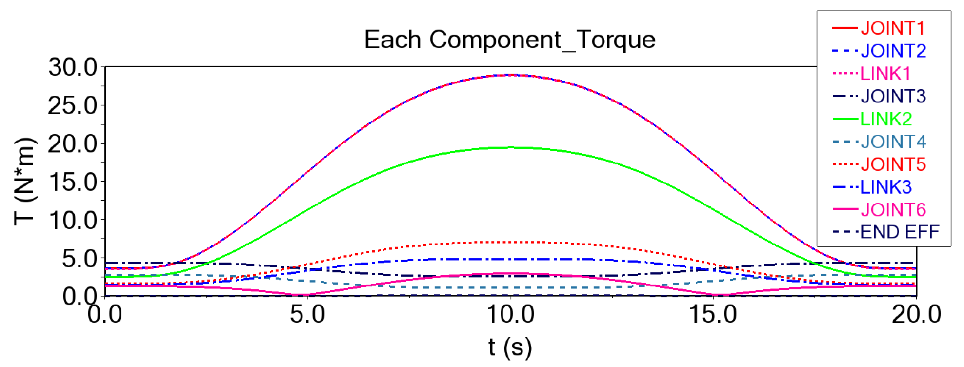
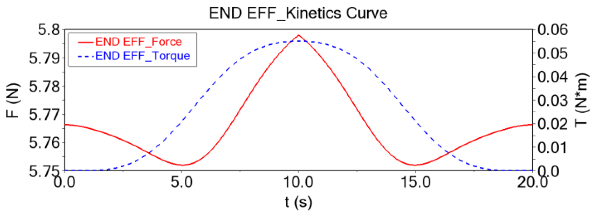
5.4. Dynamic Analysis and Simulation of Modular Reconfigurable Manipulator

To further investigate the dynamics of the forces and moments at the end-joint of the designed modular reconfigurable manipulator, a simplified proportional dynamics model is developed to obtain the kinematic and dynamic curves of the end-effector. First, kinematic relationships are defined for each manipulator component, as shown in the 6-degree-of-freedom virtual prototype in Figure 33. The gravity field is assumed to be vertically downward at the base, with each module made of 7075 aluminum alloy. The mass of each module is determined based on its geometry, and moments of inertia are generated accordingly. Next, rotation drives are applied to each joint module. The simulation time is set to 20 s with a step size of 0.01. The first 10 s simulate the manipulator’s movement from the initial to the target position, while the last 10 s simulate the return to the initial position. The motion to the target rotational joint angle is set as $\left[{\displaystyle \frac{\pi }{3}}, {\displaystyle \frac{\pi }{6}}, {\displaystyle \frac{\pi }{6}},-{\displaystyle \frac{\pi }{2}},-{\displaystyle \frac{\pi }{3}}, {\displaystyle \frac{\pi }{3}}\right]$, and the return to the initial position is also set as $\left[-{\displaystyle \frac{\pi }{3}},-{\displaystyle \frac{\pi }{6}},-{\displaystyle \frac{\pi }{6}}, {\displaystyle \frac{\pi }{2}}, {\displaystyle \frac{\pi }{3}},-{\displaystyle \frac{\pi }{3}}\right]$, with the requirement that the acceleration variation is uniform. Finally, a simulation analysis is performed for the end-effector under gravity-only conditions without a load.

Figure 34 and Figure 35 show two sets of positive kinematic curves: one for the center of mass and the other for the end-effector angle. The kinematic curves are smooth and continuous, with no abrupt changes. This indicates that the designed manipulator can perform tasks reliably and without issues. Comparing these with the kinematic curves generated using motion planning, we conclude that the sixth joint aligns with the intended motion law requirements.

The simulation also provides dynamic curves showing the force and moment changes of the end-effector and each component under no-load conditions, as depicted in Figure 36 and Figure 37. The forces and moments on the end-effector module, ordered according to the connection sequence of the manipulator’s modules, are shown along the longitudinal axis. Figure 38 shows the force and moment of the end-effector module under no-load conditions. The kinematic curve is smooth and continuous, reflecting the actual working process of the 6-degree-of-freedom manipulator. This confirms that its motion is reasonable and reliable, and that the load capacity of each module meets the design requirements. Furthermore, the force and moment experienced by the joint modules increase as they move closer to the base, with the highest values observed in joint modules 1 and 2. These are the critical components for strength, stiffness, and mechanical calibration. Therefore, the dynamic simulation analysis provides not only the force and moment change curves of each component during motion under gravity alone but also serves as a reference for the strength and stiffness assessment of the manipulator.

6. Conclusions

• This paper proposes the creation of a modular reconfigurable manipulator module library and the structural design of a new modular docking mechanism, based on the target design requirements. The modules are connected via the docking mechanism, which has been verified to enable rapid assembly and disassembly while ensuring the strength and stiffness of the connection. This enhances the reconfigurability and flexibility of the manipulator.
• This paper proposes a fast kinematic model for a modular reconfigurable manipulator that satisfies the Pieper criterion configuration and provides a method for solving both forward and inverse kinematics. The workspace is further subdivided into smaller subspaces to conduct a spatial analysis of the manipulator’s dexterity using the workspace density method. Two methods—joint space planning and Cartesian space planning—are used to generate and simulate the motion paths, successfully verifying the rationality of the manipulator’s kinematics. Finally, the dynamic simulation provides the force and moment change curves for each component during movement under gravity alone, corresponding to the kinematic curves obtained from the path planning. This also serves as a reference for strength calibration and further verifies the reasonableness of the manipulator’s kinematics while completing the dynamics analysis. The results of this paper provide valuable guidance and a reference for the design and research of plug-and-play, highly integrated modular reconfigurable manipulators.

In future work, the types of joint modules in the module library could be expanded and integrated with topology theory for optimized configuration design; additionally, systematic control algorithms tailored for diverse configurations should be further investigated to enhance modular adaptability and performance.

References

1. Surappa, S.; Pavagada, S.; Akin, D.; Wei, C.; Degertekin, F.L.; Demirci, U. Dynamically reconfigurable acoustofluidic metasurface for subwavelength particle manipulation and assembly. Nat. Commun. 2025, 16, 494. [Google Scholar] [CrossRef] [PubMed]
2. Song, S.; Gong, D.; Zhu, M.; Zhao, Y.; Huang, C. Data-Driven Optimal Tracking Control for Discrete-Time Nonlinear Systems with Unknown Dynamics Using Deterministic ADP. IEEE Trans. Neural Netw. Learn. Syst. 2023, 36, 1184–1198. [Google Scholar] [CrossRef] [PubMed]
3. Seo, J.; Paik, J.; Yim, M. Modular reconfigurable robotics. Annu. Rev. Control Robot. Auton. Syst. 2019, 2, 63–88. [Google Scholar] [CrossRef]
4. Zhu, M.; Briot, S.; Chriette, A. Sensor-based design of a delta parallel robot. Mechatronics 2022, 87, 102893. [Google Scholar] [CrossRef]
5. Dai, Y.; He, S.; Nie, X.; Rui, X.; Li, S.; He, S. Research on reconfiguration strategies for self-reconfiguring modular robots: A review. J. Intell. Robot. Syst. 2024, 110, 47. [Google Scholar] [CrossRef]
6. Liang, G.; Wu, D.; Tu, Y.; Lam, T.L. Decoding modular reconfigurable robots: A survey on mechanisms and design. Int. J. Robot. Res. 2024, 02783649241283847. [Google Scholar] [CrossRef]
7. Sarker, A.; Islam, T.U.; Islam, R. A Review on Recent Trends of Bioinspired Soft Robotics: Actuators, Control Methods, Materials Selection, Sensors, Challenges, and Future Prospects. Adv. Intell. Syst. 2024, 7, 2400414. [Google Scholar] [CrossRef]
8. Dokuyucu, H.İ.; Özmen, N.G. Achievements and future directions in self-reconfigurable modular robotic systems. J. Field Robot. 2023, 40, 701–746. [Google Scholar] [CrossRef]
9. Zhu, M.; Huang, C.; Song, S.; Xu, S.; Gong, D. Vision-admittance-based adaptive RBFNN control with a SMC robust compensator for collaborative parallel robots. J. Frankl. Inst. 2024, 361, 106538. [Google Scholar] [CrossRef]
10. Tang, S.; Huang, R.; Zhao, G.; Wang, G. Cone–hole docking mechanism for a modular reconfigurable mobile robot and its characteristic analysis. Ind. Robot. Int. J. Robot. Res. Appl. 2023, 50, 781–792. [Google Scholar] [CrossRef]
11. Xue, Z.; Liu, J.; Wu, C.; Tong, Y. Review of in-space assembly technologies. Chin. J. Aeronaut. 2021, 34, 21–47. [Google Scholar]
12. Jiang, Z.; Cao, X.; Huang, X.; Li, H.; Ceccarelli, M. Progress and development trend of space intelligent robot technology. Space Sci. Technol. 2022, 2022, 9832053. [Google Scholar]
13. Post, M.A.; Yan, X.T.; Letier, P. Modularity for the future in space robotics: A review. Acta Astronaut. 2021, 189, 530–547. [Google Scholar]
14. Zhang, Z.; Li, X.; Li, Y.; Hu, G.; Wang, X.; Zhang, G.; Tao, H. Modularity, reconfigurability, and autonomy for the future in spacecraft: A review. Chin. J. Aeronaut. 2023, 36, 282–315. [Google Scholar]
15. Li, B.; Qiu, S.; Ye, H.; Guo, Y.; Wang, H.; Bai, J. Motion planning for 7-degree-of-freedom bionic arm: Deep deterministic policy gradient algorithm based on imitation of human action. Eng. Appl. Artif. Intell. 2025, 140, 109673. [Google Scholar]
16. Blatnický, M.; Dižo, J.; Gerlici, J.; Sága, M.; Lack, T.; Kuba, E. Design of a robotic manipulator for handling products of automotive industry. Int. J. Adv. Robot. Syst. 2020, 17, 1729881420906290. [Google Scholar] [CrossRef]
17. Quan, Y.; Zhao, C.; Lv, C.; Wang, K.; Zhou, Y. The dexterity capability map for a seven-degree-of-freedom manipulator. Machines 2022, 10, 1038. [Google Scholar] [CrossRef]
18. Zhao, X.; Zhao, Z.; Liu, Y.; Su, C.; Meng, J. Analysis of workspace boundary for multi-robot coordinated lifting system with rolling base. Robotica 2024, 42, 3657–3674. [Google Scholar]
19. Cao, W.; Li, S.; Cheng, P.; Ge, M.; Ding, H.; Lai, J. Design and development of a new 4 DOF hybrid robot with Scara motion for high-speed operations in large workspace. Mech. Mach. Theory 2024, 198, 105656. [Google Scholar]
20. Ye, L.; Xiong, G.; Zeng, C.; Zhang, H. Trajectory tracking control of 7-DOF redundant robot based on estimation of intention in physical human-robot interaction. Sci. Prog. 2020, 103, 0036850420953642. [Google Scholar]
21. Wei, Y.; Zheng, Z.; Li, Q.; He, J. A trajectory planning method for the redundant manipulator based on configuration plane. Int. J. Adv. Robot. Syst. 2021, 18, 17298814211058558. [Google Scholar]
22. Zhao, J.; Xu, Z.; Zhao, L.; Li, Y.; Ma, L.; Liu, H. A novel inverse kinematics for solving repetitive motion planning of 7-DOF SRS manipulator. Robotica 2023, 41, 392–409. [Google Scholar]
23. Wang, H.; Zhao, Q.; Li, H.; Zhao, R. Polynomial-based smooth trajectory planning for fruit-picking robot manipulator. Inf. Process. Agric. 2022, 9, 112–122. [Google Scholar]
24. Potter, H.; Kern, J.; Gonzalez, G.; Urrea, C. Energetically optimal trajectory for a redundant planar robot by means of a nested loop algorithm. Elektron. Elektrotech. 2022, 28, 4–17. [Google Scholar]
25. Zeng, C.; Yang, C.; Jin, Z.; Zhang, J. Hierarchical impedance, force, and manipulability control for robot learning of skills. IEEE/ASME Trans. Mechatron. 2024. [Google Scholar] [CrossRef]
26. Fan, Z.; Jia, K.; Zhang, L.; Zou, F.; Du, Z.; Liu, M.; Cao, Y.; Zhang, Q. A cartesian-based trajectory optimization with jerk constraints for a robot. Entropy 2023, 25, 610. [Google Scholar] [CrossRef]
27. Li, X.; Zhao, H.; He, X.; Ding, H. A novel cartesian trajectory planning method by using triple NURBS curves for industrial robots. Robot. Comput. Integr. Manuf. 2023, 83, 102576. [Google Scholar]
28. Ekrem, Ö.; Aksoy, B. Trajectory planning for a 6-axis robotic arm with particle swarm optimization algorithm. Eng. Appl. Artif. Intell. 2023, 122, 106099. [Google Scholar]
Figure 1. Assembled configurations of four modular reconfigurable manipulators (1—Base; 2—Link module; 3—End-effector; 4—Docking mechanism module; 5—Joint module).
Mathematics 13 01103 g001
Figure 2. Composition of each configuration module.
Mathematics 13 01103 g002
Figure 3. Cross-section of the internal structure of the joint module (1—Joint end cap; 2—Main control board protective cover; 3—Encoder; 4—Brake adapter; 5—Motor stator; 6—Motor rotor; 7—Harmonic reducer; 8—Bluetooth module protective cover; 9—Docking fixed head; 10—Coil protective cover; 11—Magnetic coil; 12—Bluetooth module isolation plate; 13—Bluetooth module; 14—Torque sensor; 15—Torque sensor adapter; 16—Reducer adapter; 17—Motor rotor adapter; 18—Deep groove ball bearing; 19—Elastic retaining ring; 20—Brake; 21—Encoder grating; 22—Encoder mounting bracket; 23—Main control board; 24—Joint casing; 25—Torque sensor housing; 26—Docking moving head).
Mathematics 13 01103 g003
Figure 4. Two of the most demanding load conditions.
Mathematics 13 01103 g004
Figure 5. Selection Scheme for Key Components of the Joint Module.
Mathematics 13 01103 g005
Figure 6. Internal electrical and communication connections of the joint module.
Mathematics 13 01103 g006
Figure 7. Hollow wiring layout of the joint module.
Mathematics 13 01103 g007
Figure 8. Overall assembly model of the docking mechanism module.
Mathematics 13 01103 g008
Figure 9. Exploded assembly model of the docking mechanism module (1—Locking head; 2—Hand-tight bolt; 3—Active head; 4—Fixed head; 5—Magnetic coil end cap; 6—Spring pin cover; 7—Spring; 8—Spring pin; 9—Magnetic coil).
Mathematics 13 01103 g009
Figure 11. Locking holes and locking heads on the active and fixed heads of the docking mechanism module.
Mathematics 13 01103 g011
Figure 12. Locking head assembly cross-sectional view.
Mathematics 13 01103 g012
Figure 13. Overall deformation of the manipulator.
Mathematics 13 01103 g013
Figure 14. Stress map of the manipulator.
Mathematics 13 01103 g014
Figure 15. Docking mechanism module deformation diagram.
Mathematics 13 01103 g015
Figure 16. Docking mechanism module stress cloud.
Mathematics 13 01103 g016
Figure 17. Deformation diagram of the locking head.
Mathematics 13 01103 g017
Figure 18. Stress cloud of the locking head.
Mathematics 13 01103 g018
Figure 19. Kinematic model of a 6-degree-of-freedom modular reconfigurable manipulator.
Mathematics 13 01103 g019
Figure 20. Coordinate systems of each module. (a) Base module; (b) End module; (c) Intermediate assembly 1; (d) Intermediate assembly 2.
Mathematics 13 01103 g020
Figure 21. Workspace range of a 6-degree-of-freedom manipulator.
Mathematics 13 01103 g021
Figure 22. Subspace division of the workspace of a 6-DOF manipulator.
Mathematics 13 01103 g022
Figure 23. 6-DOF manipulator workspace density distribution map.
Mathematics 13 01103 g023
Figure 25. Path generated by the joint space trajectory planning method.
Mathematics 13 01103 g025
Figure 26. The joint angle variation curves of the joint space trajectory planning method.
Mathematics 13 01103 g026
Figure 27. The joint angular velocity variation curves of the joint space trajectory planning method.
Mathematics 13 01103 g027
Figure 28. The joint angular acceleration variation curves of the joint space trajectory planning method.
Mathematics 13 01103 g028
Figure 29. Paths generated using the Cartesian spatial trajectory planning method.
Mathematics 13 01103 g029
Figure 30. Angle variation curves for each joint in the Cartesian spatial trajectory planning method.
Mathematics 13 01103 g030
Figure 31. Angular velocity variation curves for each joint in the Cartesian spatial trajectory planning method.
Mathematics 13 01103 g031
Figure 32. Angular acceleration variation curves for each joint in the Cartesian spatial trajectory planning method.
Mathematics 13 01103 g032
Figure 33. Virtual prototype of the modular reconfigurable manipulator with 6 degrees of freedom.
Mathematics 13 01103 g033
Figure 34. End-effector module kinematics curve 1.
Mathematics 13 01103 g034
Figure 35. End-effector module kinematics curve 2.
Mathematics 13 01103 g035
Figure 36. The force conditions of each module under no-load conditions.
Mathematics 13 01103 g036
Figure 37. The torque conditions of each module under no-load conditions.
Mathematics 13 01103 g037
Figure 38. End-effector module kinetic curves.
Mathematics 13 01103 g038