Abstract
To address environmental challenges, governments globally have implemented a range of carbon reduction policies. Based on their mechanisms of action, this study categorizes these policies into regulatory (e.g., carbon taxes and cap-and-trade) and supportive measures (e.g., production cost subsidies, low-carbon technology subsidies, and low-carbon product subsidies). By integrating these approaches, six distinct policy combinations were identified. A supply chain network equilibrium model, incorporating manufacturers, retailers, and demand markets, was developed using variational inequality theory to assess the effectiveness of these combinations. Numerical simulations were conducted with a modified projection algorithm, and the Borda method was applied to evaluate equilibrium outcomes, specifically production levels and emission reductions, under each policy combination, revealing synergies between policies. The analysis revealed three key findings: (1) Among supportive policies, the combination of low-carbon product subsidies with regulatory policies is the most effective, while production cost subsidies are relatively weaker; (2) carbon tax policies combined with supportive policies outperform carbon trading; (3) a higher intensity of regulatory policies enhances the incentive effects of supportive policies. This research offers valuable guidance for governments seeking to design evidence-based policy portfolios that effectively balance emission reduction goals with economic development priorities.
Keywords:
carbon tax policy; carbon trading policy; government subsidies; low-carbon supply chain network equilibrium; variational inequality MSC:
90C33; 49J40; 90B06; 91A10
1. Introduction
Over the past few decades, global dependence on fossil fuels, such as coal and oil, for industrial production and economic growth has significantly increased carbon dioxide emissions. Since 1751, the world has released over 1.5 trillion tons of carbon dioxide, intensifying global warming. To limit the average temperature rise to 2 degrees Celsius, urgent international efforts are essential to curb emissions. In response to this challenge, the Paris Agreement was adopted at the 21st United Nations Climate Change Conference in December 2015. Concurrently, governments worldwide have established carbon reduction targets. For instance, Austria and Iceland aim for carbon neutrality by 2040, while the United Kingdom, the United States, France, and South Korea target 2050. In 2020, China announced its dual carbon goals: peaking emissions by 2030 and achieving neutrality by 2060.
To meet these objectives, nations are designing policies to regulate the carbon emissions of industries, enterprises, and individuals. The most widely adopted measures include carbon tax policy and carbon trading policy. However, challenges such as limited funding, outdated equipment, and insufficient technology often undermine corporate motivation, rendering emission reduction efforts formidable. Therefore, to address these issues effectively, governments pair regulatory policies with subsidy policies to incentivize energy efficiency and emission cuts. In Australia, states and local governments have introduced subsidies to encourage investment in the photovoltaic industry. Similarly, in Canada, some provinces have implemented the “Climate Action Incentive Fund”, which enables enterprises to receive government subsidies of up to 25% of the investment cost when they actively invest in green technologies (including photovoltaic, hydropower, and wind power). The specific subsidy amount ranges from 20,000 to 250,000. In conclusion, governments have designed and introduced various policies to achieve carbon emission reduction targets. Broadly, there are mainly two types of policies: regulatory low-carbon policies designed from the perspective of regulation and constraint; and supportive low-carbon subsidy policies designed from the perspective of incentives and support. Due to the complementarity between the two approaches, many regions and countries implement these policies in parallel. For instance, the European Union employs the Emissions Trading System (EU ETS) to set emission quotas, while supplementing it with low-carbon subsidies to encourage green innovation and technological upgrades among enterprises. Compared to a single type of policy, this integrated approach leverages synergistic effects, ensuring mandatory enforcement while stimulating corporate proactivity through incentives. This not only achieves environmental goals but also alleviates economic burdens on businesses, fostering coordinated development of the economy and the environment. In light of this dual approach, a natural question arises: which combination of regulatory and supportive policies has a better synergy effect?
In recent years, scholars have conducted initial explorations on various subsidies under different carbon policies. However, their research has predominantly focused on a two-tier supply chain consisting of a manufacturer and a retailer. Additionally, the evaluation of carbon policy and government subsidies usually focuses solely on the criterion of “carbon emission reduction”. In fact, with economic globalization, modern supply chains are usually characterized by multi-level, multi-actor, cross-cutting, and cross-regional networks. Moreover, governments, in addition to pursuing environmental improvements, also emphasize various development goals such as economic growth and income distribution. To the best of our knowledge, the coordinated development between economy and environment remains a central issue in driving sustainable economic transformation. Nevertheless, there are limited studies that have explored the synergy between different regulatory and supportive low-carbon policies while simultaneously integrating economic and environmental considerations within a multitiered supply chain network structure.
In view of this research gap, this study models supply chain enterprises as profit-maximizing decision-makers driven by economic rationality. The government, characterized by its non-profit nature and public regulatory functions, is treated as an exogenous policy variable. Through policy instruments that act on manufacturers, the government seeks to influence decision-making across supply chain entities. Therefore, we establish a low-carbon supply chain network comprising multiple manufacturers, retailers, and demand markets. Within this framework, this study establishes six policy scenarios combining regulatory policies (carbon taxation and emissions trading) with supportive subsidy policies (low-carbon product subsidies, production cost offsets, and green technology incentives). Based on these combination scenarios, we formulate profit maximization functions for enterprises through an economic behavioral analysis of supply chain entities. A supply chain network equilibrium model is then constructed using variational inequalities to characterize multi-agent interactions. For governments, the profitability of supply chains provides the economic foundation for policy implementation, determining the feasibility of emission reduction measures. Meanwhile, carbon mitigation performance serves as the cornerstone of the environmental objectives, directly influencing progress toward carbon peaking and neutrality targets. Accordingly, this paper evaluates the synergistic effects of policy combinations using economic indicators, such as the profits of decision-making entities, and environmental indicators, including the low-carbon level of products and total emission reductions. In the numerical simulations, the equilibrium solutions across multiple indicators are computed for the six policy combinations using a modified projection algorithm. A multi-criteria decision-making framework, based on the Borda count method, is then employed to identify the policy combination with the best overall performance. Furthermore, sensitivity analysis is conducted to assess how key policy parameters such as subsidy rates, carbon tax rates, and carbon quotas affect policy synergy. This study elucidates policy synergy effects by analyzing corporate production and emission abatement performance across heterogeneous policy portfolios, providing actionable insights to enhance regulatory implementation efficacy and balance industrial decarbonization with economic growth.
The rest of this paper is organized as follows: Section 2 reviews the relevant literature and describes the motivation of this paper; Section 3 develops an equilibrium model of the supply chain network under three government subsidy schemes, paired with either carbon tax or carbon trading policies, and presents the optimal conditions for network equilibrium using variational inequalities. Section 4 explores the existence, uniqueness, and numerical algorithms of the equilibrium solution of the supply chain network; Section 5 analyzes the effects of policy parameter changes on policy synergy through numerical examples and sensitivity analysis. Section 6 summarizes the findings and provides corresponding management insights.
2. Literature Review
In recent years, the research on carbon tax policy and carbon trading policy has attracted extensive attention from scholars worldwide. Concurrently, studies exploring production and emission reduction decisions in low-carbon supply chains under these policies have proliferated, yielding substantial insights. This section reviews the relevant research progress across three dimensions: carbon tax policy, carbon trading policy, and subsidy policy for low-carbon supply chains.
2.1. Research Related to Carbon Tax Policy
Regarding carbon tax policies, studies have mainly explored the production and emission reduction decisions of low-carbon supply chains under different tax scenarios, such as single-ratio carbon tax, interval tax, and over-progressive carbon tax. For example, ref. [1] constructed an international supply chain with upstream suppliers and downstream manufacturers to examine how changes in carbon tax rates affect manufacturers’ decisions to produce in-house or outsource, under both single-ratio and interval tax scenarios. Ref. [2] analyzed the effects of a progressive carbon tax on pricing and emission reduction strategies within a two-channel supply chain. He also explored how consumer channel preferences impact equilibrium decisions, carbon emissions, and profits. In the context of closed-loop supply chains, ref. [1] compared equilibrium decisions under single proportional and highly progressive carbon taxes. Ref. [3] investigated the influence of three distinct carbon tax policies on power generation decisions in a closed-loop supply chain operating within carbon quota constraints. Additionally, ref. [4] developed an oligopolistic supply chain network model to assess how different carbon tax policies (including single proportional, progressive, and emission limitation regulations) affect equilibrium outcomes. Based on the aforementioned literature, it is evident that existing research predominantly focuses on classifying carbon tax types and analyzing their effects on enterprise decision-making, emission reductions, and economic outcomes under various tax frameworks. However, there remains a significant research gap in integrating carbon tax policies with subsidy mechanisms and evaluating their potential synergistic effects.
2.2. Related Research on Carbon Trading Policy
Regarding carbon trading policies, existing studies have primarily concentrated on the development of carbon quotas and carbon prices and their impact on supply chain decisions. Ref. [2] integrated carbon trading centers into a closed-loop supply chain model to examine how carbon quotas and variations in remanufacturing recovery rates influence firms’ production and emission reduction strategies. Ref. [5] constructed a closed-loop supply chain network equilibrium equilibrium model by considering firms’ non-compliance with carbon trading policies. Ref. [6] constructed a supply chain network equilibrium model and conducted numerical simulations to evaluate how government-set carbon trading prices and carbon taxes affect equilibrium decisions in closed-loop supply chains. In a related study, ref. [7] modeled a closed-loop supply chain featuring multiple manufacturers, remanufacturers, and distributor/collection centers. They employed a differential game model to analyze how remanufacturing ratios impact optimal decisions under carbon emission permit systems. Furthermore, ref. [8] established game models between original manufacturers and remanufacturers under various scenarios: carbon trading policy, a historical emission-based approach, and a benchmark-based approach. Their analysis focused on how different carbon quota allocation methods influence manufacturing and remanufacturing supply chains. Based on the aforementioned literature, it is evident that the current research on carbon trading policy predominantly centers on carbon quotas, carbon prices, and quota allocation methods. However, few studies have integrated these policies with government subsidies to investigate their combined effects on emission reduction effectiveness and environmental benefits from multiple perspectives.
2.3. Study on Subsidy Policy in Low-Carbon Supply Chain
In recent years, with the increasing environmental awareness of consumers, there has been a surge in research related to consumer green preferences and government subsidy policies in low-carbon supply chains. Ref. [9] analyzed a two-tier supply chain, employing a manufacturer-led Stackelberg game model to assess how subsidies for manufacturers, retailers, or consumers influence decision-making among supply chain agents. Ref. [10] established a government-led Stackelberg model considering the consumer green preferences over time. Their analysis examined how these dynamic green preferences and various government subsidy objectives impact supply chain decisions. Ref. [11] categorized consumer quality preferences and product greenness into distinct levels and proposed differentiated subsidies based on product greenness. Their research further investigated how consumer quality preferences influence product greenness and production decisions. Ref. [12] explored a two-tier supply chain comprising manufacturers and retailers by constructing four Stackelberg models. Their work compared the effects of subsidies under both manufacturer-led and retailer-led scenarios on supply chain decisions. Additionally, ref. [13] proposed three manufacturer-focused subsidy types: covering production costs, abatement investments, and low-carbon products. They further utilized Stackelberg models to evaluate their effectiveness under equal expenditure conditions while accounting for consumer green preferences. In summary, the above studies mainly focus on two-tier supply chains involving a single manufacturer and retailer, emphasizing decision-making under a given subsidy approach. However, there is limited research examining the effects of different government subsidies within more complex supply chain networks that incorporate multiple manufacturers, retailers, and demand markets.
2.4. Research Contributions
To better describe the contribution of this paper, we compare it with the existing literature, as summarized in Table 1. By reviewing the literature mentioned above, it is evident that previous studies have mainly focused on exploring the impact of a single low-carbon policy on corporate decision-making. However, in practice, multiple emission reduction policies are often implemented concurrently. There exists a notable deficiency in the in-depth classification of carbon reduction policies and the comprehensive analysis of their combined effects. Moreover, research on low-carbon policy impacts predominantly focuses on single supply chain structures. In reality, as the number of supply chain members increases and relationships among them become more complex, supply chains have expanded in both vertical and horizontal dimensions, evolving into the current complex network structure characterized by multiple actors and hierarchical levels. Based on the above comprehensive analysis, the major research gaps are summarized from two aspects as follows:

Table 1.
Characteristics of the relevant literature of low-carbon supply chain design.
First, distinct from research on corporate decision-making under single-policy contexts, we categorize carbon mitigation policies into regulatory and supportive mechanisms based on directional effects: regulatory policies compel emission reductions through cost internalization (e.g., carbon tax) or emission caps (e.g., emission trading), whereas supportive policies incentivize proactive decarbonization initiatives via economic stimulus like low-carbon subsidies. We then construct six policy combinations by pairing two regulatory policies (carbon tax and carbon trading) with three supportive subsidy policies (targeting production costs, low-carbon technologies, and low-carbon products). Subsequently, this paper examines how these combinations influence enterprise production and emission reduction strategies, revealing their synergistic effects.
Second, in contrast to policy research based on single-chain supply structures, this paper considers a multitiered supply chain network comprising multiple manufacturers, retailers, and demand markets. By employing variational inequality theory, we formulate the non-cooperative, profit-maximizing behaviors of multiple agents as variational inequality problems. This mathematical framework rigorously captures the competitive dynamics of low-carbon and pricing strategies among intra-tier and cross-tier decision-makers, thereby enhancing the operational relevance of policy design in complex supply chain ecosystems.
To summarize, by using variational inequality theory, this study constructs a multitiered supply chain network framework to analyze enterprise production and emission abatement strategies under six policy portfolios (combining regulatory and supportive instruments). It evaluates the synergistic effects of these policy combinations from the perspectives of environmental and profit performance, reveals the combined effects and synergistic mechanisms of the policies, and thereby enhances the effectiveness of policy implementation and promotes the balance between emission reduction and economic development.
3. A Low-Carbon Supply Chain Network Equilibrium Model Considering Carbon Policy and Government Subsidies
In this section, we first outline the topology of the supply chain network. We then develop its equilibrium model, incorporating three distinct types of government subsidies: subsidies for emission reduction investments, for production cost reduction, and for low-carbon products. Subsequently, we analyze this model under two carbon policy frameworks: the carbon tax policy and the carbon trading policy.
3.1. Description of the Problem and Related Symbols
The low-carbon supply chain network studied in this paper consists of M manufacturers, R retailers, and K demand markets, where the manufacturer m () is responsible for the R&D, production, packaging, and transportation of low-carbon products to the retailer r (); retailers r further sell low-carbon products to the demand market k (). The topology of this supply chain network is depicted in Figure 1.
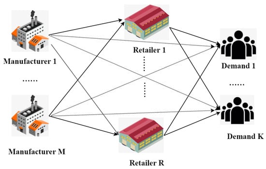
Figure 1.
Supply chain network topology.
In reality, there are many practical cases where regulatory carbon policies (carbon trading and carbon taxes) are implemented concurrently with supportive carbon policies (subsidies for low-carbon products, low-carbon technologies, and production costs). For example, China’s national carbon market (ETS) currently imposes emissions caps on the power sector. Additionally, the Ministry of Industry and Information Technology’s (MIIT) Special Plan for Industrial Green Development proposes “special green development subsidies”. These subsidies aim to provide energy-intensive industries, such as steel and cement, with funds for upgrading their production processes to save energy, thereby offsetting their low-carbon transition costs. Moreover, Japan imposes the “Global Warming Countermeasure Tax”, which is a carbon tax. A portion of its revenue is channeled into the “Green Innovation Fund”. This fund provides R&D subsidies to enterprises, accelerating advancements in key technologies like next-generation batteries and hydrogen-based steelmaking. Furthermore, in order to incentivize corporate emission reduction, the government provides subsidies to enterprises based on the low-carbon level of their products. France’s Climate Energy Tax, which is a carbon tax, covers industrial emissions. Additionally, the “Low-Carbon Building Certification (E+C-)” system offers procurement premium subsidies of up to 15% for certified low-carbon building materials, such as low-carbon cement, in government purchases. This initiative drives the marketization of low-carbon product premiums.
Based on the aforementioned practical examples, in the supply chain network, governments serve as exogenous regulatory entities. They implement regulatory policies, such as carbon taxes or carbon trading, to oversee manufacturers. Simultaneously, to incentivize manufacturers to actively product green and low-carbon products, the government implements three types of subsidies: subsidies for production costs, subsidies for investment in emission reduction, and subsidies for low-carbon products, with the corresponding subsidy rates denoted as , , and , respectively. Obviously, when the subsidy rates , , and are 0, it means that the government has not taken the corresponding subsidy.
The above low-carbon supply chain network inherently constitutes a non-cooperative game-theoretic system involving multiple rational decision-makers (manufacturers, retailers, demand markets). Each participant aims to maximize their own profit or utility within their strategy space, which includes decisions such as production volume, pricing, and emission reduction investments. However, their optimal decisions are directly influenced by the strategic choices of other participants. This equilibrium state precisely captures the steady-state dynamics, reflecting both competition and cooperation within multi-agent supply chain systems. It thus offers a formal analytical framework for deconstructing complex network interactions. Consequently, in order to construct the supply chain network equilibrium model under different policy combinations, this paper further proposes the following assumptions:
Assumption 1.
A non-cooperative game is played among low-carbon supply chain entities located in the same tier. The objective of all low-carbon supply chain entities is to maximize profit (utility). The decision variables for these entities, along with their definitions, are detailed in Table 2;
Table 2.
Symbols and related descriptions.
Assumption 2.
All manufacturers produce homogeneous goods, although they differ in scale. To accurately reflect the impact of carbon reduction policies, all manufacturers are considered high-emission enterprises;
Assumption 3.
The government sets different carbon tax rates and carbon quota allocations for each manufacturer;
Assumption 4.
All cost functions and demand functions are continuously differentiable convex functions, and they all have bounded second-order partial derivatives;
Assumption 5.
The emission reduction investment of the manufacturer m is denoted as T, and it is assumed that this emission reduction investment is a quadratic function of the carbon emission reduction level per unit of the product. In the absence of carbon policies and emission reduction investments, the carbon emission per unit of product is . However, considering carbon policies and emission reduction investments, the carbon emission per unit of product becomes . In addition, due to natural factors and technological limitations, the unit carbon emission of the product cannot be lower than the minimum unit carbon emission . Therefore, the unit carbon emission should satisfy the relationship: . Consequently, it is easy to know that the product’s The level of carbon emission reduction per unit can be expressed as . Assume that the cost function of emission reduction investment satisfies the expression , where denotes the initial fixed investment, and κ the investment scale factor [20].
3.2. Supply Chain Network Equilibrium Model Considering Carbon Tax Policy and Government Subsidies
In this section, we examine how government policies, which are carbon taxes and subsidies, shape the behavior of entities within the low-carbon supply chain. The analysis centers on identifying the optimal conditions for manufacturers and the optimal conditions for retailers, as well as understanding the equilibrium conditions in the demand market. Based on these insights, we construct an equilibrium model of the supply chain network that incorporates the effects of both carbon tax policies and government subsidies.
3.2.1. Behavior of Manufacturers and Optimality Conditions
Under the implementation of carbon tax policies by the government, the decision variables for the manufacturer m are as follows: the total quantity of products produced , the quantity of products wholesaled to retailer r denoted as , and the carbon emission reduction per unit of product . Since cannot exceed the total number of products produced by the manufacturer m, satisfies the following condition:
In addition, according to Assumption 5, for any manufacturer m, the unit carbon emission of the low-carbon products produced satisfies the following condition:
Furthermore, since the decision variables of manufacturer mm are non-negative, we have the following:
The above (1) to (3) consider the constraints that need to be satisfied by the decision variables of manufacturer m. Now, let us establish the profit function for manufacturer m. To do so, we first consider the three subsidy schemes that the government provides to manufacturer m.
Subsidy Scheme 1. The government provides subsidies for the carbon emission reduction investments of manufacturer m. In this case, the government subsidizes the emission reduction investment of the manufacturer m at a subsidy rate , so that denotes the emission reduction investment of the manufacturer m after deducting the subsidy, as follows:
Subsidy Scheme 2. The government provides subsidies for the production costs of manufacturer m. In this case, the government subsidizes the production cost of manufacturer m at a subsidy rate . Let denote the actual production cost of the manufacturer after the subsidy, as follows:
Subsidy Scheme 3. The government provides subsidies for the carbon emission reduction benefits of manufacturer m. To characterize the carbon emission reduction benefits of manufacturer m, let k be the monetary value per unit of carbon emission reduction (). The total revenue generated from producing units of product is k(). In this case, the government subsidizes k() at a subsidy rate of . Let be the subsidy amount received by manufacturer m, as follows:
In addition to the government subsidy mentioned above, under the carbon tax policy, manufacturer m is also required to pay a carbon tax per unit of carbon emissions generated from its production activities. Let denote the total amount of carbon tax paid by manufacturer m, as follows:
Let denote the profit of the manufacturer m. The decision problem for manufacturer m is to find to maximize its profit, as follows:
According to Assumption 1, manufacturers play a non-cooperative game with a Nash equilibrium portrayed by the following Definition 1. At this point, each manufacturer chooses its own optimal strategy given its competitors’ strategies, and each manufacturer is unwilling to unilaterally change its strategy.
Definition 1.
If the following inequality (9) holds for each manufacturer m; , then the vector , composed of product production quantities, trade quantities, and low-carbon levels, constitutes a Nash equilibrium.
where , , , represents the strategy set of manufacturer m, .
Given the complex functional form of the aforementioned Nash equilibrium problem, obtaining a closed-form solution is generally challenging. In recent years, transforming this problem into a variational inequality and subsequently employing numerical methods has proven to be an effective approach for solving such problems [21].
Lemma 1.
Suppose that is an optimal solution to the convex optimization problem , Ω is a closed convex set, and is continuously differentiable. Then, is a solution to the following variational inequality problem:
where represents the gradient function of at , .
Theorem 1.
(Variational Inequality Formulation of the Manufacturer’s Nash Equilibrium Considering Carbon Tax and Government Subsidies). Assume that M manufacturers compete in a non-cooperative manner, and the cost function, trade function, and emission reduction investment function are all continuously differentiable convex functions. According to the concept of Nash equilibrium in Definition 1, the optimality conditions for all manufacturers simultaneously can be expressed as the following variational inequality: determine satisfying
where , , , and are the Lagrange multipliers corresponding to constraints (1) to (3). All , , and form vectors μ, ξ, and ς, respectively. That is, , , and .
Proof.
Since we assume that all involved cost functions are continuously differentiable covex functions, then is a continuously differentiable convex function with respect to , , and , and the strategy set is a convex set, the profit maximization problem for every manufacturer can be transformed into a convex optimization problem. In the Nash equilibrium state, manufacturer m reaches the optimal condition at to maximize its profit. According to Lemma 1, in this case, its convex optimization problem , can be transformed into a variational inequality. Therefore, the convex optimization problem for the M manufacturers can be transformed into the variational inequality (11) mentioned above. □
According to Theorem 1, when the manufacturers make optimal decisions, the wholesale price can be obtained by solving the first term in Equation (11): . From the second term, we have . Therefore, we can conclude that the wholesale price decision is influenced by the marginal transaction cost, production cost subsidy rate, marginal production cost, carbon tax rate, and unit carbon emissions.
3.2.2. Behavior of Retailers and Optimality Conditions
For retailer r, the decision variables are the quantity of products purchased from manufacturer m and the quantity of products sold to the demand market k from . Obviously, satisfies the following condition:
Since all decision variables are non-negative, therefore
The cost for retailer r to purchase products from manufacturer m is . The total holding cost, including display, storage, and so on, incurred from selling products to the consumer market, is .
Let be the profit of retailer r. The decision problem faced by retailer r is to find and that maximize its profit, as follows:
Similar to manufacturers, retailers in a supply chain network play a non-cooperative game, meaning that each retailer seeks to maximize its profit given the behavior of the other retailers.
Theorem 2.
(Variational Inequality Formulation of the Nash Equilibrium for Retailers under the Carbon Tax Policy). Assume that the product holding cost function is a continuous convex function and that R retailers compete in a non-cooperative manner. Then, the optimality condition when all retailers reach equilibrium can be expressed as the following variational inequality: determine satisfying the following:
where , and represents the Lagrange multiplier corresponding to the constraint (12). All form the vector v, that is, .
Proof.
The proof process is similar to Theorem 1. □
From (15), it can be observed that in the equilibrium state, . From the second term, it can be inferred that , which means that an increase or decrease in wholesale price will affect the retailer’s selling price. This reflects the transitivity of prices, and ultimately, the market bears the final prices.
3.2.3. The Optimality of the Demand Market
In the demand market k, consumers need to purchase low-carbon products from retailers. In addition to paying the price of the product, they also need to pay the sum of various costs incurred from the transaction. The demand market k satisfies the following complementary equilibrium conditions:
Equation (16) indicates that transactions between the retailer and the demand market occur only when consumers’ willingness to pay exceeds the retail price. Moreover, Equation (17) reveals that a positive price in the demand market signifies that such transactions are taking place, and consequently, the quantity of products sold by the retailer equals the market demand.
Theorem 3.
(Variational Inequality Formulation of the Demand Market under the Carbon Tax Policy) For markets k; , if conditions (16) and (17) are both satisfied, then all markets reach equilibrium, and the equilibrium condition for the demand market can be transformed into the following variational inequality: determine satisfying the following:
where .
3.2.4. The Equilibrium Conditions of the Supply Chain Network Considering Carbon Tax and Government Subsidy Policies
When the supply chain network achieves equilibrium, the quantity of products delivered from each manufacturer to each retailer must correspond precisely to the quantity received by the retailer from the manufacturer. Similarly, the quantity of products purchased by consumers in the demand market must be equal to the quantity of products sold by the retailer to the demand market. The formal definition of equilibrium in the supply chain network is presented below.
Definition 2.
(Multitiered Supply Chain Network Equilibrium under Carbon Tax Policy) Under a carbon tax policy, if the product flows between different levels of decision-making entities are mutually consistent, and the product flows and prices satisfy the sum of variational inequalities (11), (15), and (18), then a multitier supply chain network with subsidies reaches an equilibrium state.
Theorem 4.
(Variational Inequality Formulation of the Multitiered Supply Chain Network Equilibrium). Under the carbon tax policy, the optimality conditions of a supply chain network with a subsidy policy to reach equilibrium are equivalent to the following variational inequality problem: determine satisfying the following:
where .
3.3. Supply Chain Network Equilibrium Model Considering Carbon Trading Policy and Government Subsidies
3.3.1. Behavior of Manufacturers and Optimality Conditions
Now, we discuss the behavior and optimal conditions of low-carbon supply chain subjects under carbon trading policy and government subsidies. In this case, the government aims to encourage companies to reduce emissions and energy consumption by implementing three types of subsidies for manufacturers. On the other hand, manufacturers are required to produce within the carbon quota set by the government. If they exceed their allocated carbon allowance, they need to purchase the excessive carbon emissions, denoted as , from the carbon trading center at a carbon price plus a commission . The cost incurred for purchasing carbon emission rights is denoted as , as follows:
In addition, the carbon emissions of manufacturer m are equal to the sum of the purchased carbon emission rights and the carbon quota provided by the government, satisfying the constraint:
Under the carbon trading policy, the decision variables of manufacturer m remain unchanged, and they still satisfy the constraint conditions (1), (2), and (3). Similar to the carbon tax policy, we still consider the three types of subsidies and satisfy Equations (4), (5), and (6). Let represent the profit of manufacturer m under the carbon trading policy. Combining the cost analysis in Equation (20) with the constraint (21), we can formulate the profit maximization problem for manufacturer m as follows:
Theorem 5.
(Variational Inequality Formulation of the Manufacturer’s Nash Equilibrium Problem Considering Carbon Trading and Government Subsidies). Assuming that the cost functions for production, transaction, and carbon abatement investment in the utility function are all convex, and manufacturers compete in a non-cooperative manner and reach Nash equilibrium, then the Nash equilibrium problem of this game can be expressed by the following variational inequality: find , such that
where , is the Lagrange multiplier corresponding to constraint (21), and all form the vector ζ, that is, .
Proof.
The proof process is similar to Theorem 1. □
Since both the carbon policy and the subsidy policy are implemented only on manufacturer entities, the optimality conditions for retailers and demand markets under the carbon trading policy are exactly the same as in Section 3.2.
3.3.2. The Equilibrium Conditions of the Supply Chain Network Considering Carbon Trading and Government Subsidy Policy
When carbon trading and government subsidies are introduced, equilibrium within the supply chain network is attained when product flows between manufacturers, retailers, and the demand market are balanced. Specifically, the volume of products dispatched by manufacturers must equal the volume received by retailers. Similarly, the quantity purchased by consumers in the demand market must match the quantity sold by retailers. The formal definition of this equilibrium state, incorporating the effects of carbon trading and government subsidies, is presented below.
Definition 3.
(Multitiered Supply Chain Network Equilibrium under Carbon Trading Policy). Under the carbon trading policy, if the product flows between different decision-making entities are mutually consistent, and the product flows and prices satisfy the sum of variational inequalities (23), (15), and (18), then a multitier supply chain network with subsidies reaches an equilibrium state.
Theorem 6.
(Variational Inequality Formulation of the Multitiered Supply Chain Network Equilibrium). In the context of carbon trading and government subsidies, the equilibrium conditions for the supply chain network model are equivalent to the solution of the variational inequality problem given by determining satisfying the following:
where .
4. Qualitative Analysis and Numerical Algorithms for Supply Chain Network Equilibrium Model Considering Carbon Policies and Government Subsidies
This section commences with an investigation into the existence and uniqueness of solutions for the supply chain network equilibrium model under various carbon policies. Subsequently, iterative algorithms designed for solving the supply chain network equilibrium model will be introduced, accompanied by an analysis of their convergence properties.
4.1. Qualitative Analysis
4.1.1. Existence of a Solution
Lemma 2.
If Ω is a compact convex set in , and the vector function that enters the variational inequality is continuous on this compact convex set, then the variational inequality admits at least one solution .
In this paper, we take the variational inequality (19) as an example. Let , and is
where . Then, the variational inequality in Theorem 4 can be transformed into (25).
Definition 4.
Theorem 7.
Proof.
Since the cost functions in this paper have bounded second-order partial derivatives, and the demand price functions have bounded first- and second-order partial derivatives, according to the mean value theorem for derivatives, there exists a constant (which is the Lipschitz constant) such that the function that enters the variational inequalities (19) and (24) is Lipschitz continuous. □
Theorem 8.
Proof.
The existence of the solution is discussed in the following example of the supply chain network equilibrium model (19) under the carbon tax policy. Due to the non-compactness of the feasible set , in order to ensure the existence of solutions, we adopt a method widely used in the study of supply chain network equilibrium [21], which imposes a relatively weak boundary condition on the feasible region. We analyze it as follows:
where , and means that for all m, r, k. Then, is a bounded closed convex subset of . Let , under the premise that is a closed convex set, and the gradient function is continuous, according to Lemma 2; then, there exists a feasible solution to the variational inequality (19) on , which can be represented by the following Equation (37).
Therefore, combining the Lipschitz continuity analysis in Theorem 7 and the construction of the compact convex set in Theorem 8, we can infer from Lemma 2 that the variational inequality (19) admits at least one solution. □
The existence of solutions for model (24) follows the same analysis as above.
4.1.2. Uniqueness of the Solution
Lemma 3.
Suppose that is strictly monotone on ; then, the solution to is unique, if one exists.
Definition 5.
is said to be locally strictly monotone at if there is a neighborhood of such that
is strictly monotone at if the above inequality holds true for all . is said to be strictly monotone if the above inequality holds for all x,, .
Theorem 9.
(Monotonicity). Since the functions , , , and involved in the model are all continuous convex functions, and the demand function is a monotonically decreasing function of for all m and k, according to Definition 5, the vector functions that enter the variational inequalities (19) and (24) are strictly monotone functions; that is, , and the following inequality (39) holds.
Proof.
In Equation (19), let , , where the left-hand side of the variational inequality (19) can be expressed in the following form:
Equation (40) consists of six terms, denoted in order as , , , , , and .
Since the retailer’s product holding cost function , the production cost function , the transaction cost function , and the emission reduction cost function are all continuous and convex functions, it follows that , , , and are all greater than zero. The transaction cost function between the retailer and the consumer market is strictly monotonically increasing, so is positive. Moreover, the demand function is a strictly monotonically decreasing function with respect to the consumer payment price , so is positive. Thus, the variational inequality (19) is greater than zero on the closed convex set . □
According to Lemma 3, the analysis of Theorems 8 and 9 leads to the fact that the variational inequality (19) has a unique feasible solution on .
Similarly, the variational inequality (24) also has a unique feasible solution.
4.2. The Modified Projection Method
Iteration Steps and Convergence Analysis
To address the variational inequality presented in Section 3, this paper employs the modified projection algorithm introduced by Korpelevich [22]. Widely recognized for its effectiveness in solving variational inequalities [21], this iterative method involves two primary steps in each iteration: prediction and adaptation. The procedure of the algorithm, with iterations indexed by the counter t, is detailed below.
Step 1. Initialization
Initialize with . Set and select , such that , where L is the Lipschitz constant.
Step 2. Prediction
Step 3. Adaptation
Step 4. Convergence Verification
If , for , a pre-specified tolerance level, then stop; otherwise, set t:= , and go to Step 1.
The convergence of the model of this paper under this algorithm is discussed below.
Lemma 4.
Theorem 10.
Proof.
From the above analysis, it can be concluded that the vector function that enters variational inequalities (19) and (24) is strictly monotone (Theorem 9) and Lipschitz continuous (Theorem 7). Moreover, there exists a feasible solution for the variational inequalities (19) and (24) on a closed convex set. Therefore, based on Lemma 4, the convergence of the algorithm is already proven. □
5. Numerical Examples
This section begins with the definition of cost functions and parameters, ensuring all cost functions adhere to Assumption 4. These parameters and functions are then incorporated into Models (19) and (24). Using the modified projection algorithm described in Section 4.2, we conduct iterative computations with MATLAB 2017a software to obtain the equilibrium solutions. Finally, through qualitative comparisons of equilibrium outcomes, we derive relevant management insights.
To assess the synergistic effects of various policy combinations while reflecting the government’s balanced emphasis on environmental benefits and economic efficiency, this study assigns equal weights to environmental and economic indicators. Building on this principle, the Borda count method is applied for comprehensive evaluation. Developed by the 18th-century French mathematician Jean-Charles de Borda in 1770, the Borda Count is a ranked voting system in which options are assigned scores according to their ranking positions, with the highest total score indicating the optimal choice. The Borda count method has several advantages. First, it considers voters’ complete ranking preferences, which can lead to more representative and stable outcomes. Second, it encourages candidates to appeal to a broader electorate rather than just focusing on their core supporters. Third, it reduces the likelihood of strategic voting and vote splitting, promoting a more fair and efficient electoral process.
As a simple and objective multi-criteria ranking method, the Borda method eliminates the need for subjective weighting. It synthesizes the ranked scores of policy combinations across evaluation dimensions (e.g., corporate profitability, low-carbon product performance). This approach effectively circumvents the subjectivity controversies inherent in traditional weighted-sum approaches, which are caused by arbitrary weight allocation. Therefore, it is highly suitable for assessing policy synergy effects characterized by multiple objectives and conflicting priorities. In our case study, the evaluation process using the Borda method is as follows: First, policy combinations are ranked according to their required subsidy amounts for achieving equivalent indicator values. Subsequently, scores are assigned based on these rankings. Finally, the total scores across all indicators are computed, and the policy combination with the highest score is identified as the most effective in terms of combined impact.
5.1. Introduction of the Case Background
The following sections focus on the low-carbon supply chain depicted in Figure 2, which consists of one manufacturer (), two retailers (), and two demand markets (). The relevant cost functions and demand functions are shown in Table 3. Let , , , , , , and . Regarding the parameters in the iterative algorithm, let and , and all examples are solved using the modified projection method.
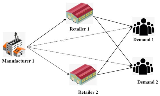
Figure 2.
Supply chain network topology of the case study.
Table 3.
The definitions of related functions.
In this case, the three subsidy methods specifically refer to subsidies for emission reduction investment technologies, production costs, and low-carbon products.
The differentiated cost functions of retailer 1 and retailer 2 reflect their competitive relationship. The differentiated demand functions of the two markets reflect the preferences for the same product in different demand markets.
5.2. Analysis of the Synergistic Effect of Carbon Emission Reduction Policy and Subsidy Policy
To quantify the environmental benefits resulting from reduced carbon emissions, “environmental benefits” are defined as the product of per-unit carbon emission reduction and the quantity of products. Consequently, environmental benefits are positively correlated with both per-unit carbon emission reduction and product quantity. Since per-unit carbon emission reduction is equivalent to the original carbon emissions minus the unit carbon emissions, a smaller unit carbon emission value results in greater carbon reduction, thereby enhancing environmental benefits. In other words, environmental benefits increase as per-unit carbon emissions decrease. Under carbon tax and carbon trading policies, the government’s selection of subsidy methods significantly affects not only the economic outcomes for itself and supply chain participants but also the environmental benefits by influencing emission levels.
To evaluate the effectiveness of different subsidy methods, this section uses the following evaluation criteria: manufacturer profit, retailer profit, per-unit product carbon emissions, environmental benefits, and tax revenue. Within the frameworks of carbon tax and carbon trading policies, the response of these criteria to variations in subsidy rates is analyzed. Subsequently, the optimal subsidy method corresponding to each evaluation criterion is discussed. Finally, the Borda method is employed to conduct a multi-criteria evaluation of the three subsidy methods, integrating the results across all criteria to determine the optimal approach.
In this section, it is assumed that the subsidy rates of the three types of subsidies vary within the interval (0, 0.3), the carbon tax rate = 0.2, and the carbon quota . For simplicity, the subsidized emission reduction investment approach, the subsidized production cost approach, and the subsidized low-carbon product approach are denoted as , , and , respectively. For bt1, bt2, bt3}, let represent the manufacturer profit under subsidy method , represents the retailer profit under subsidy method , represents the unit carbon emissions under subsidy method , represents the environmental benefits under subsidy method , and represents the subsidy amount corresponding to subsidy method , and represents the subsidy amount corresponding to subsidy method .
5.2.1. Analysis of Synergistic Effects of Carbon Tax Policy and Three Subsidy Policies
- (1)
- Synergies of carbon tax policy and three subsidy policies, and the impact of subsidy rate on manufacturers’ profits
The computational results for this scenario are shown in Figure 3. From the graph (b), it can be observed that under the carbon tax policy, for each subsidy method , the manufacturer’s profit is incremental with the increase in subsidy rate. Furthermore, at the same subsidy rate, the manufacturer profit satisfies the condition: . While initially appears to be the optimal subsidy method concerning manufacturer profit, it is crucial to recognize that, at the same subsidy rate, the subsidy amounts for the three methods differ. Consequently, comparing manufacturer profits under a uniform subsidy rate is insufficient for evaluating the effectiveness of the subsidy methods.
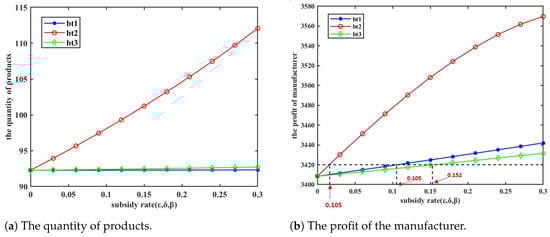
Figure 3.
Changes in production quantity and manufacturer profit under carbon tax policy ().
To explore this issue from an alternative perspective, we investigate which subsidy method minimizes the required subsidy amount to achieve a specified level of manufacturer profit. Evidently, for an equivalent “output” (manufacturer’s profit), the subsidy method requiring the lowest “input” (subsidy amount) is optimal. For instance, if the target manufacturer’s profit is set to 3420, the corresponding subsidy amounts for the three subsidy methods are presented in Table 4:
Table 4.
Subsidies corresponding to the three subsidy methods when ( = 0.2).
From Table 4, it can be concluded that when the manufacturer’s profit is 3420, the subsidy amounts for the three methods can be compared as follows: bt2bt1bt3). Therefore, it can be inferred that the subsidy for low-carbon products () is the most beneficial for the manufacturer’s profit. When the manufacturer’s profit takes on other values, a similar analysis can be conducted, and the ranking results will remain consistent.
- (2)
- Synergies of carbon tax policy and three subsidy policies, and the impact of subsidy rate on retailers’ profits
The computational results for this scenario are presented in Figure 4. Figure 4 reveals that subsidizing production costs leads to a substantial increase in the retailer’s profit curve, whereas the profit curves under the other two subsidy methods exhibit no significant changes. A detailed analysis of Figure 3a further indicates that manufacturers’ production costs significantly exceed both the investment required for emission reductions and the economic returns from low-carbon products. Therefore, under the same subsidy rate, the amount of subsidy for production costs will be much higher than the subsidies for the other two methods. This, in turn, incentivizes manufacturers to produce a larger volume of products, thereby driving a rapid increase in retailers’ profits.
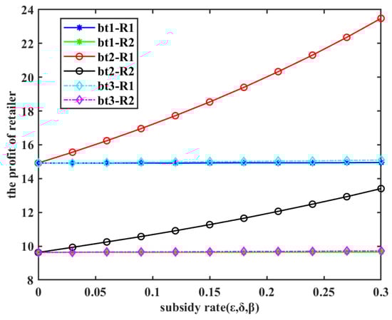
Figure 4.
The change in retailer profits under the carbon tax policy ().
Similar to Scenario 1, when the subsidy rates of the three subsidy methods are the same, the corresponding subsidy amounts are generally different. Consequently, comparing retailer profits at the same subsidy rate is not a reliable basis for evaluating the effectiveness of these methods. Therefore, we first arbitrarily select a value for the retailer’s profit and then determine which subsidy method corresponds to the minimum subsidy amount. For example, when the retailer’s profit is set to 15, the corresponding subsidy amounts for the three subsidy methods are shown in Table 5:
Table 5.
Subsidies corresponding to the three subsidy methods when ( = 0.2).
From Table 5, when the retailer’s target profit is 15, the result of the comparison of the subsidy amount of the three approaches is as follows: . Therefore, the subsidized low-carbon product strategy is the most beneficial for the retailer’s profit. When the retailer’s profit takes other values, it can be analyzed similarly and the ranking results remain consistent.
- (3)
- Synergies of carbon tax policy and three subsidy policies, and the impact of subsidy rates on carbon emission reduction per unit
The computational results for this scenario are presented in Figure 5. This figure reveals that all three subsidy methods incentivize manufacturers to reduce emissions. Notably, subsidizing low-carbon products results in a significant decrease in the unit carbon emissions curve, whereas the rate of decline for this curve is comparatively slower under the other two methods.
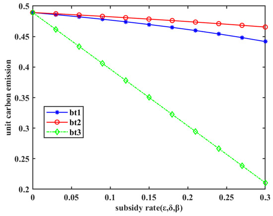
Figure 5.
The change in unit carbon emissions under carbon tax policy ().
To evaluate the relative effectiveness of the subsidy methods in incentivizing emission reductions, a specific value for unit carbon emissions is arbitrarily selected, and the corresponding subsidy amounts for the three methods are compared. This comparison allows for an assessment of the efficacy of each subsidy method in reducing unit carbon emissions. For example, when a unit of carbon emissions is selected as 0.46, the corresponding subsidy amounts for the three subsidy methods are shown in Table 6.
Table 6.
Subsidies corresponding to the three subsidy methods when ( = 0.2).
Based on Table 6, it can be observed that when the unit carbon emissions are 0.46, the required subsidy amounts for the three subsidy methods satisfy the following condition: . Given that a lower subsidy amount signifies higher subsidy efficiency, and considering the results presented in Figure 5, it can be concluded that the subsidy for low-carbon products strategy has the most optimal incentive effect on unit carbon emission reduction. Similar analysis can be conducted for other values of unit carbon emissions, and the ranking of subsidy methods remains consistent.
- (4)
- Synergies of carbon tax policy and three subsidy policies, and the impact of subsidy rates on environment revenue
The calculation results for this scenario are shown in Figure 6. From the graph, it can be observed that for each subsidy method , as the subsidy rate increases, the environmental benefits exhibit an upward trend. Notably, the subsidy method for low-carbon products demonstrates the most substantial increase in environmental benefits.
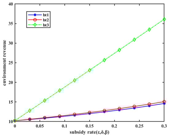
Figure 6.
The change in environment revenue under carbon tax policy ().
To assess which subsidy method is more effective in enhancing environmental benefits, a specific environmental benefit value is selected as a target, and the minimum subsidy amount required for each subsidy method to achieve that target is examined. For instance, if the target environmental benefit value is set to 14, the corresponding subsidy amounts for the three subsidy methods are presented in Table 7:
Table 7.
Subsidies corresponding to the three subsidy methods when ( = 0.2).
From Table 7, we can see that when the environmental benefit is 14, the subsidy amounts for the three subsidy methods satisfy the following relation: . As a smaller subsidy amount indicates higher efficiency, combined with Figure 6, it can be concluded that the subsidy method for low-carbon products () has the most optimal incentive effect on improving the environment. When considering other values of environmental benefits, a similar analysis can be conducted, and the ranking results will remain consistent.
- (5)
- Synergies of carbon tax policy and three subsidy policies, and the impact of subsidy rates on carbon tax revenue
The calculation results for this scenario are shown in Figure 7. The figure illustrates that the trend in government tax revenue varies across the three subsidy methods as the subsidy rate increases. Specifically, under the subsidy method of subsidizing production costs (), the government’s carbon tax revenue steadily increases. However, for the other two subsidy methods, the government’s taxable amount gradually decreases with the increase in subsidy rate, which demonstrates that subsidizing production costs () is the optimal approach for the government to enhance carbon tax revenue.
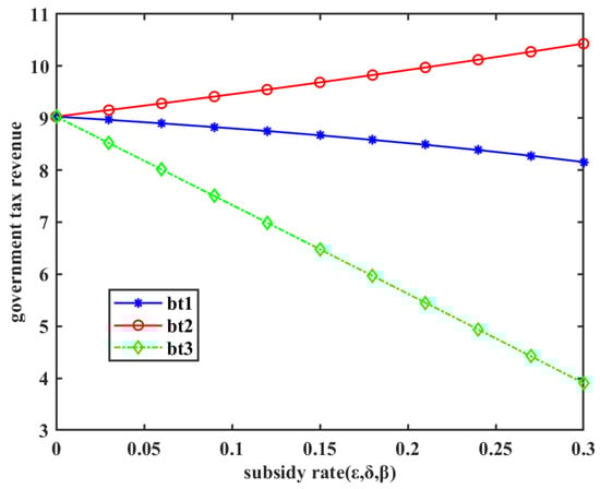
Figure 7.
The change in government tax revenue under carbon tax policy ().
Next, a specific carbon tax value is selected to evaluate the merits and demerits of the different subsidy methods. The subsidy amounts corresponding to the three subsidy methods are then compared at this specified tax value. For instance, when the government sets the carbon tax amount to 8, the corresponding subsidy amounts for the three subsidy methods are presented in Table 8.
Table 8.
Subsidies corresponding to the three subsidy methods when bt ( = 0.2).
From Table 8, it can be seen that when the government sets the target carbon tax amount to 8, the corresponding subsidy amounts for the two subsidy methods satisfy the condition: . Because a smaller subsidy amount indicates a more favorable subsidy method, it can be concluded, in combination with Figure 7, that subsidizing production costs () is the optimal strategy for government carbon tax revenue.
- (6)
- Multi-criteria evaluation of the three subsidy methods under carbon tax policy
Previously, under the carbon tax policy, we explore the advantages and disadvantages of three subsidy methods based on five criteria: manufacturer’s profit, retailer’s profit, carbon emissions per unit, environmental benefits, and carbon tax revenue. The results indicate that the ranking of the three subsidy methods varies depending on the evaluation criteria considered. The sorting results are shown in Table 9, where the numbers in each column represent the ranking of the corresponding subsidy method under that criterion.
Table 9.
Ranking of the three subsidy methods for each criterion under carbon tax policy ( = 0.2).
In the real world, selecting the optimal subsidy method often requires considering multiple criteria simultaneously. Therefore, the selection of subsidy methods is essentially a multi-criteria decision-making problem. It is worth noting that Table 9 provides the ranking results of the three subsidy methods under different criteria. Hence, this paper adopts the Borda method to evaluate subsidy methods under multiple criteria [23]. According to the Borda method, values are assigned based on the rankings of the different subsidy methods under each criterion. The subsidy method ranked first receives a score of 3, the second receives a score of 2, and the third receives a score of 1. This process yields the scores for each subsidy method for each criterion, as presented in Table 10. Subsequently, the scores for each subsidy method across all criteria are summed to obtain a total score. Finally, the subsidy methods are comprehensively ranked based on these total scores.
Table 10.
Scores of the three subsidy methods under carbon tax policy ().
From Table 10, it can be observed that under the carbon tax policy, the subsidy method for low-carbon products () achieves the highest total score. This indicates that this subsidy method has the best overall performance.
For the sake of visual representation, the data in Table 10 can be plotted as Figure 8. By observing the radar chart of the scores for each subsidy method, we can see that the subsidy strategy for low-carbon products has high scores in terms of manufacturer profit, retailer profit, unit carbon emissions, and environmental benefits. However, it has a lower score in terms of government taxation potential. On the other hand, the other two subsidy methods have lower scores in all aspects. Therefore, combining the results from Table 10, the subsidy for low-carbon products strategy demonstrates a balanced and optimal subsidy effect.
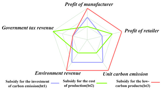
Figure 8.
Radar chart evaluating the three subsidy methods under carbon tax policy ().
The calculation of the overall scores for the subsidy methods above did not incorporate the weights of each criterion. In reality, decision-makers can assign different weights to different criteria based on their needs, resulting in weighted total scores. Currently, there are various methods available for assigning weights, such as the Analytic Hierarchy Process (AHP) [24], Entropy Weight Method [25], Best–Worst Method (BWM) [26], and so on.
5.2.2. Analysis of the Synergistic Effects of Carbon Trading Policy and Three Subsidy Policies
This section examines the effects of three subsidy methods on manufacturers’ profits, retailers’ profits, unit carbon emissions, and environmental benefits under the carbon trading policy. Furthermore, we explore the optimal subsidy methods under various evaluation criteria.
- (1)
- Synergies of carbon trading policy and three subsidy policies, and the impact of subsidy rates on manufacturers’ profit
Figure 9 illustrates that, under the carbon trading policy, manufacturers’ profits rise with increases in both production costs and subsidies for emission reduction investments. However, variations in the subsidy rate for low-carbon products do not significantly affect manufacturers’ profits.
Figure 9.
Changes in production quantity and manufacturer profit under carbon trading policy ().
Consistent with the findings in Section 5.2.1, when the subsidy rates for the three methods are equivalent, the actual subsidy amounts differ. Consequently, comparing manufacturer profits at a uniform subsidy rate does not reveal the most optimal subsidy method. Therefore, this paper investigates the minimum subsidy amount required to achieve a predetermined level of manufacturer profit. Logically, a lower subsidy amount is preferable when manufacturer profits are held constant. For instance, if a target manufacturer profit of 3430 is set, the necessary subsidy amounts for each method are presented in Table 11.
Table 11.
Subsidies corresponding to the three subsidy methods when ( = 25).
According to Table 11, it can be observed that when the manufacturer profit is 3430, the required subsidy amounts for the three subsidy methods satisfy . Therefore, under the carbon trading policy, the subsidy strategy for emission reduction investment () has the most optimal incentive effect on manufacturer profits, followed by the subsidy strategy for low-carbon products (), while the subsidy strategy for production costs () shows the poorest effect. When the manufacturer’s profit takes other values, it can be analyzed similarly, and the results of the ranking of the incentive effects of the subsidy methods remain consistent.
- (2)
- Synergies of carbon trading policy and three subsidy policies, and the impact of subsidy rates on retailers’ profit.
Figure 10 demonstrates that as the subsidy rate increases, the trend in retailer profits across the three subsidy methods mirrors that observed in Figure 4. Consequently, the ranking of the three subsidy methods, with respect to retailer profits, remains consistent with the findings presented in Table 5.

Figure 10.
Changes in retailer’s profit under carbon trading policy ().
- (3)
- Synergies of carbon trading policy and three subsidy policies, and the impact of subsidy rates on unit carbon emission
From Figure 11, it can be observed that when adopting the subsidy method for production costs, as the subsidy rate increases, the manufacturer’s per-unit carbon emissions significantly decrease. However, under the other two subsidy methods, the per-unit carbon emissions remain around 0.27.
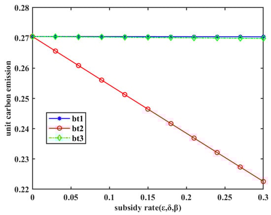
Figure 11.
Changes in unit carbon emission under carbon trading policy ().
To explore the incentive effects of the three subsidy methods under the criterion of per-unit carbon emissions, a specific value for per-unit carbon emissions is selected, and the corresponding subsidy amounts for each method are examined. For example, if we set the per-unit carbon emissions to 0.27, the computational results are shown in Table 12. The subsidy amounts corresponding to the three subsidy methods satisfy . Since a smaller subsidy amount indicates a better subsidy method, it can be concluded that under this policy, the subsidy method for production costs () has the most optimal incentive effect on reducing per-unit carbon emissions. A similar analysis conducted with alternative values for unit carbon emissions consistently produces the same ranking of incentive effects among the subsidy methods.
Table 12.
Subsidies corresponding to the three subsidy methods when ( = 25).
- (4)
- Synergies of carbon trading policy and three subsidy policies, and the impact of subsidy rates on environment revenue
Figure 12 illustrates that, when subsidizing production costs, environmental benefits increase significantly with a rising subsidy rate. However, the remaining two subsidy methods exhibit negligible changes in environmental benefits. This trend aligns with the variation observed in Figure 11. A similar analysis, conducted with alternative values for unit carbon emissions, consistently maintains the same ranking of effectiveness among the subsidy methods.
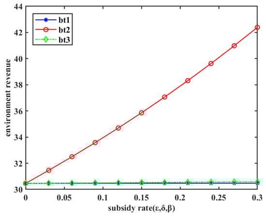
Figure 12.
Changes in environment under carbon trading policy ().
To evaluate the three subsidy methods with respect to environmental benefits, a benchmark environmental benefit of 30.5 is established, and the corresponding subsidy amounts for each method are compared. The results are shown in Table 13. It can be observed that when the environmental benefit is 30.5, the required subsidy amounts for the three methods satisfy the following order: . Therefore, in terms of environmental benefits, subsidizing low-carbon products () yields the best results, followed by subsidizing emission reduction investments (), while subsidizing production costs () proves to be the least effective.
Table 13.
Subsidies corresponding to the three subsidy methods when ( = 25).
- (5)
- Government tax revenue under carbon trading policy
Because manufacturers are averse to incurring additional costs for carbon emissions under all three subsidy methods, they will constrain their emissions to within the government-mandated quota, irrespective of the chosen subsidy approach. Consequently, manufacturers have no incentive to purchase carbon emission rights from the carbon trading center, precluding the government from generating fiscal revenue through this mechanism.
- (6)
- Multi-criteria evaluation of the three subsidy methods under carbon trading policy
The preceding discussion, within the framework of a carbon trading policy, has examined the impacts of the three subsidy methods according to four criteria: manufacturer profits, retailer profits, per-unit carbon emissions, and environmental benefits. Table 14 illustrates that the ranking of the incentive effects of the three subsidy methods varies depending on the specific criterion applied.
Table 14.
Ranking of the three subsidy methods for each criterion under carbon trading policy ( = 25).
Consistent with the approach in Section 5.2.1, the Borda method is now employed to evaluate the overall effects based on the four aforementioned criteria. Initially, scores are assigned to the ranking of subsidy methods under each criterion, as presented in Table 15. Subsequently, the total scores for each subsidy method are calculated. The results indicate that subsidizing low-carbon products () yields the most favorable overall effect within the context of a carbon trading policy. In contrast to Figure 8, Figure 13 reveals that the scores for each subsidy method are not uniformly distributed, suggesting that no single subsidy method simultaneously satisfies all criteria. This radar chart enables the government to select the optimal subsidy method for each individual criterion. Nevertheless, considering the overall criteria, the strategy of subsidizing low-carbon products demonstrates superior performance.
Table 15.
Scores of the three subsidy methods under carbon trading policy ().
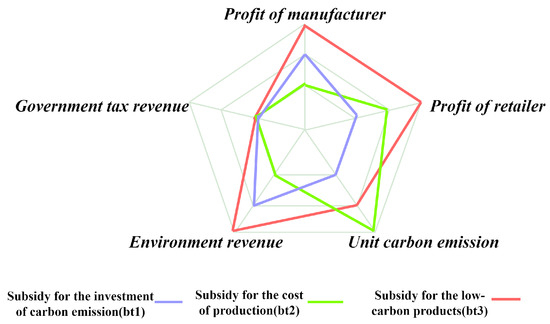
Figure 13.
Radar chart evaluating the three subsidy methods under carbon trading policy ().
5.3. Analysis of Differentiated Synergistic Effects of Carbon Emission Reduction Policies and Subsidy Policies
The preceding analysis clearly demonstrates that the three subsidy methods offer distinct incentives to decision-making entities within the supply chain. As illustrated in Table 9 and Table 14, the integration of these three subsidy methods with various emission reduction policies generates differentiated synergistic effects. Consequently, this leads to variations in the ranking of subsidy method effectiveness across all criteria, with the exception of retailer profit.
5.3.1. Analysis of the Difference in Emission Reduction Effects
The carbon tax policy requires enterprises to bear the carbon tax at a fixed rate regardless of the amount of carbon they emit. Therefore, regardless of the subsidy method adopted, companies will strictly control carbon emissions to reduce tax burdens, leading to a decrease in per-unit carbon emissions, as depicted in Figure 5.
When the government adopts the subsidy () for production costs (see the red curve in Figure 5), it can reduce the manufacturing costs and alleviate the production pressure for manufacturers. Therefore, manufacturers prioritize expanding production quantities to enhance profits over solely focusing on carbon emission reduction. As a result, the rate of reduction in per-unit carbon emissions is comparatively slower. When the government provides subsidies () for emission reduction investments to companies (see the purple curve in Figure 5), manufacturers are more willing to reduce their carbon emissions at the source in order to reduce their carbon tax burden. Hence, they achieve a relatively higher rate of carbon emission reduction. When the government provides subsidies () to companies based on the low-carbon level of products (see the green curve in Figure 5), manufacturers can directly benefit from producing high-level low-carbon products. Furthermore, the production of low-carbon products reduces the burden of carbon taxes. In this double-beneficial scenario, manufacturers are highly motivated to reduce per-unit carbon emissions. Therefore, compared to the other two subsidy methods, subsidizing low-carbon products achieves the fastest rate of carbon emission reduction.
In summary, combining with Table 6, the ranking of the three subsidy methods in terms of their effectiveness in reducing carbon emissions per unit is as follows: .
Under the carbon trading policy, manufacturers are obligated to maintain their total carbon emissions within a predetermined quota. Otherwise, they would need to purchase emission allowances from other companies with surplus emissions. Therefore, within the quota limits, companies are exempt from paying any fees. Manufacturers can maintain their carbon reduction capacity at a certain level and increase production quantities to generate higher profits, as shown in Figure 11.
When adopting the subsidy () for production costs, manufacturers will expand production. To ensure compliance with the carbon quota (i.e., total carbon emissions do not exceed the limit), manufacturers must reduce per-unit carbon emissions. By observing the changes in the red curve in Figure 11, it can be seen that the curve of per-unit carbon emissions consistently decreases with the change in subsidy rate. By observing the changes in the purple and green curves in Figure 11, it can be seen that under the subsidy ( and ) for emission reduction investments and low-carbon products, the carbon emissions per unit of product for manufacturers are maintained at around 0.2705, and the total carbon emissions of the company exactly equal the carbon quota of 25. Therefore, manufacturers have no further incentive to invest in research and development for additional carbon emission reduction.
In summary, combining with Table 12, the comparative results of the three subsidy methods in terms of their effectiveness in reducing carbon emissions per unit are as follows: .
Since environmental benefits equal the product of carbon reduction per unit and production quantity, combined with the analysis of the changes in carbon emissions per unit as mentioned above, we can explain the reasons for the changes in environmental benefits in Figure 6 and Figure 12.
Therefore, based on the goal of maximizing profits, the regulatory approach of emission reduction policies will cause changes in the emission reduction behaviors of decision-making entities in the supply chain, thus affecting the emission reduction effects of various subsidy methods. This will result in differentiated synergistic effects between different emission reduction policies and three subsidy methods.
5.3.2. Analysis of Differences in Profitability Effects
Under the carbon tax policy, manufacturers are required to pay for their carbon dioxide emissions, which increases their economic costs. By examining the profit curve in Figure 3, it can be seen that all three subsidy approaches can enhance the manufacturer’s profit.
Under the subsidy method for low-carbon products () (see the green curve in Figure 3), the increase in the manufacturer’s profit level can be attributed to two factors. Firstly, the manufacturer gains additional benefits from the government’s subsidy for low-carbon products. Secondly, the improvement in the low-carbon level reduces the burden of carbon tax. Under the subsidy method for emission reduction investments () (see the purple curve in Figure 3), the manufacturer increases its profit by investing in emission reduction, which leads to a decrease in carbon emissions. However, under the subsidy method for production costs () (see the purple curve in Figure 3), the manufacturer continues to expand production to seek profit enhancement, neglecting emission reduction efforts. The rate of income increase from increased production is lower than the rate of increasing carbon tax burden. Therefore, the effect of profit enhancement is not significant.
In summary, the comparative results of profit enhancement for the three subsidy approaches are as follows: .
Under the carbon trading policy, since manufacturers are high-emission enterprises, they will control their total carbon emissions within the carbon quota specified by the government in order to avoid additional expenses. Therefore, manufacturers would limit their production quantity and per-unit carbon emissions to a certain level, ensuring that the total carbon emissions precisely equal the carbon quota. They would no longer invest in research and development funds to reduce unit carbon emissions. As a result, all three subsidy approaches have a minimal incentive effect on profits (see Figure 9).
Therefore, similar to the analysis of emission reduction effects, the regulatory approach of emission reduction policies has led to changes in the economic behavior of supply chain decision-makers, thereby affecting the incentive effects of various subsidy approaches on profits. This results in differentiated synergistic effects when different emission reduction policies are combined with the three subsidy approaches.
5.4. The Impact of Policy Parameter Changes on the Synergistic Effects of Policy Combinations
5.4.1. The Impact of Carbon Tax Rate Changes on the Synergistic Effects
In the preceding section, the carbon tax rate was established at 0.2. This section examines the impact of intensified taxation on manufacturers by increasing the carbon tax rate to . The resulting changes in the equilibrium conditions of the supply network model under this elevated carbon tax rate are explored, with the equilibrium results presented in Figure 14.
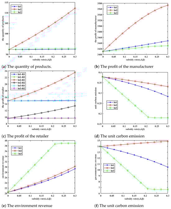
Figure 14.
Change in equilibrium results under carbon tax policy ().
A comparison of Figure 3 and Figure 6, alongside Figure 14a–f, reveals that the trends in all equilibrium results remain consistent under both carbon tax rate conditions. Additionally, the ranking of the three subsidy methods remains unchanged across various evaluation criteria. The only difference is that under a carbon tax rate of 0.4, the unit carbon emissions reach their minimum level earlier.
Under the three subsidy methods, let us compare the equilibrium results for the two carbon tax rate conditions as follows:
By observing Figure 15, Figure 16 and Figure 17, it can be concluded that under the three subsidy schemes, with the exception of retailer margins, other equilibrium results are more optimal when the carbon tax rate is 0.4. Therefore, when the carbon tax rate is increased to 0.4, the equilibrium results under all three policies change positively. From an economic perspective, manufacturers’ profits increase; from the perspective of energy saving and emission reduction, per-unit carbon emissions decrease and environmental benefits increase. Therefore, the increased taxation on manufacturers enhances the incentive effect of a given subsidy rate, promoting both economic growth for manufacturers and the development of a low-carbon environment, ultimately leading to improved synergistic effects.
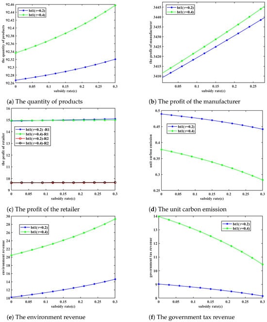
Figure 15.
Comparison of equilibrium results under the subsidy method ().
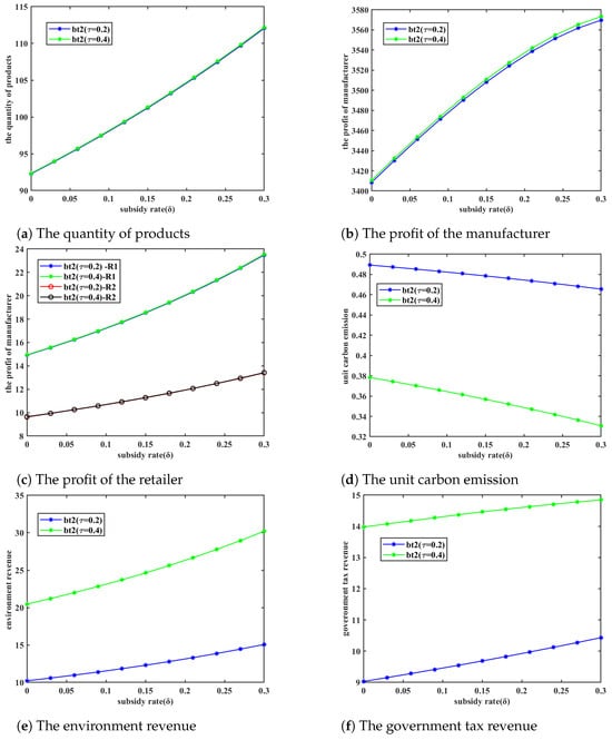
Figure 16.
Comparison of equilibrium results under the subsidy method ().
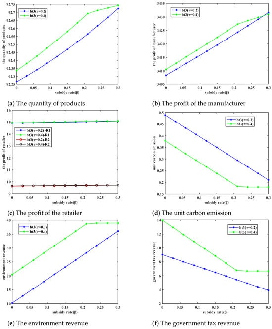
Figure 17.
Comparison of equilibrium results under the subsidy method ().
5.4.2. The Impact of Carbon Quota Changes on the Synergistic Effects
In the preceding section, the carbon quota was established at 25. This section examines the effects of increased pressure on manufacturers to reduce carbon emissions by lowering the carbon quota to 20. The resulting changes in equilibrium results under this adjusted carbon quota are explored, as presented in Figure 18.
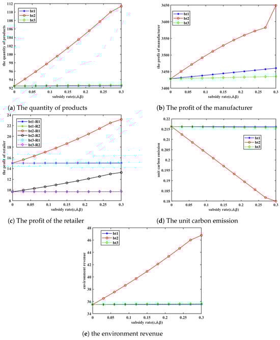
Figure 18.
Change in equilibrium results under carbon trading policy ().
A comparison of Figure 9 through Figure 12 with Figure 18a–e reveals that, under both carbon quota conditions, the trends in the various equilibrium results remain consistent as the subsidy rate increases. Additionally, the ranking of the three subsidy schemes’ effectiveness remains unchanged across various evaluation criteria.
Comparing the equilibrium results under the three subsidy schemes for the two quota scenarios, we have the following comparisons:
Observation of Figure 19, Figure 20 and Figure 21 reveals that, under the three subsidy schemes, all equilibrium results, with the exception of retailer profits, are more favorable when the carbon quota is 20. Therefore, whether from an economic perspective or an environmental perspective, increasing emission reduction pressure and reducing the carbon quota to 20 result in better synergistic effects.
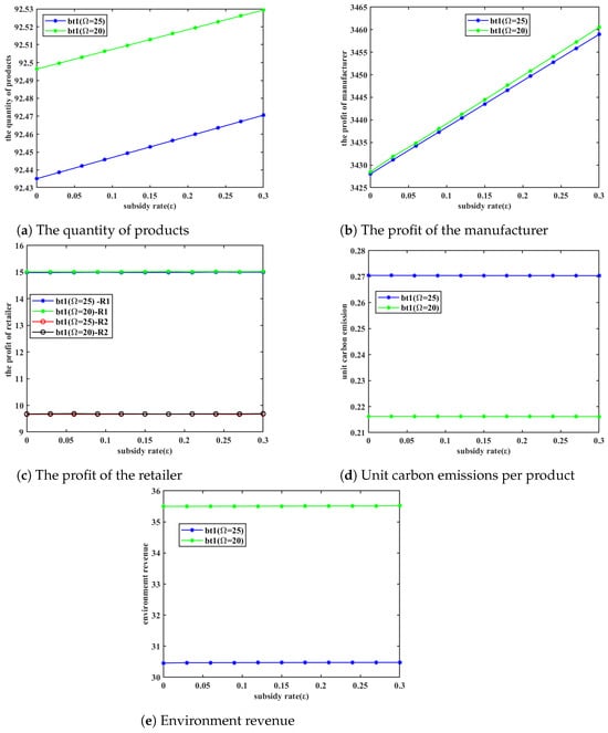
Figure 19.
Comparison of equilibrium results under the subsidy method ().
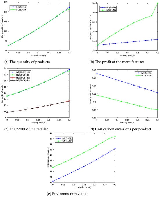
Figure 20.
Comparison of equilibrium results under the subsidy method ().
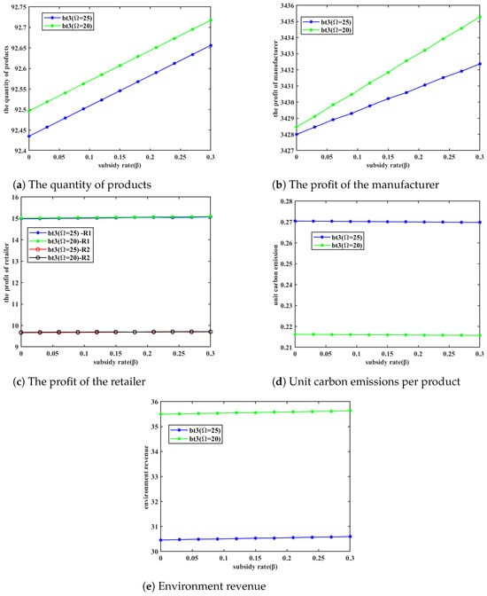
Figure 21.
Comparison of equilibrium results under the subsidy method ().
Based on the preceding analysis, it can be concluded that increasing the carbon emission burden on manufacturers, either by raising the carbon tax rate to 0.4 or reducing the carbon quota to 20, maintains the stability of the ranking of the three subsidy schemes across various evaluation criteria within the subsidy rate range of 0 to 0.3. Concurrently, both emission reduction efficiency and economic benefits exhibit improved subsidy effects under the same subsidy scheme. This alignment of manufacturers’ emission reduction goals with their economic benefit objectives fosters a more efficient low-carbon supply chain.
6. Conclusions
This paper classifies low-carbon policies into regulatory and supportive categories. A single-proportion carbon tax and a carbon trading policy represent regulatory policies. Subsidies for production costs, emission reduction R&D costs, and low-carbon products represent supportive policies. These are combined into six policy combinations. Based on the economic activities of decision-makers, profit-maximization objective functions are constructed against the background of the six policy combinations. Then, a supply chain network equilibrium model, comprising multiple manufacturers, retailers, and demand markets, is formulated using variational inequality theory. In the numerical analysis, the modified projection algorithm is used to solve for the supply chain network equilibrium under each policy combination. Based on the equilibrium solutions, the Borda method is employed to compare the economic and environmental indicators, including profits, low-carbon levels per unit product, and total emission reductions. Sensitivity analyses on the carbon tax rate and carbon quotas are further conducted. The main conclusions and management insights are as follows:
(1) Under any emission reduction policy, the three subsidy methods have certain incentive effects on the economic growth and emission reduction efforts of supply chain entities. Among them, the subsidy for low-carbon products () demonstrates the highest effectiveness, whereas the subsidy for production costs () proves the least effective. The low-carbon product subsidy () directly ties financial support to low-carbon attributes, thereby fostering technological advancements and product innovation within enterprises. This generates market-driven incentives for emission reduction, yielding optimal overall effectiveness. In contrast, the production cost subsidy () merely reduces marginal costs, potentially leading to increased production capacity without corresponding investments in emission reduction. This creates an imbalance between environmental benefits and economic gains, rendering it the least effective approach. These findings emphasize the need for policy designs that prioritize goal orientation and closely align subsidies with low-carbon outcomes to maximize their impact.
(2) Compared to carbon trading policies, the incentive effects of various subsidy schemes are more significant under carbon tax policies. Specifically, under carbon tax policies, emissions are taxed at a certain proportion. Therefore, manufacturers urgently need subsidies to encourage voluntary emission reductions and alleviate the tax burden. Consistent with the first conclusion, governments are advised to prioritize dynamic subsidy mechanisms linked to emission reduction performance, particularly within carbon tax frameworks. Concurrently, carbon trading systems should be coupled with dynamic quota adjustments. Empirical evidence demonstrates that static quota systems risk fostering allowance dependency among enterprises, undermining the effectiveness of subsidy-driven emission reduction incentives. For instance, in the UK steel industry, Tata Steel achieved only a 3.2% reduction in emissions under a carbon trading framework with fixed quotas in 2023, relying on minor technological improvements. However, when the UK implemented a 5% annual quota reduction policy alongside performance-based subsidies, Tata Steel’s Port Talbot plant achieved a 14% emission reduction through significant furnace technology upgrades. This contrast underscores the value of integrating dynamic quota constraints with targeted low-carbon subsidies to drive meaningful decarbonization.
(3) When regulatory policies intensify, such as through higher carbon taxes or reduced carbon allowances, both emission reductions and manufacturer profits increase under the three subsidy schemes. This outcome arises because stricter carbon regulations prompt governments to intensify their policies, either by elevating carbon taxes or curtailing allowances, thereby raising carbon costs and compelling manufacturers to lower their emissions. Meanwhile, subsidy policies partially transform emission reduction investments into cost advantages through their compensation effect, while the interaction between carbon pricing and product pricing creates new opportunities for profit growth. This indicates that there is alignment between the profit goals of enterprises in the supply chain network and the emission reduction goals of the government. Consequently, policymakers should devise frameworks that dynamically adjust subsidy levels in accordance with the stringency of emission controls. These frameworks should also incorporate carbon market signals to directly link subsidy adjustments to fluctuations in carbon prices. This mechanism harnesses market pressures to incentivize businesses to convert emission reduction investments into long-term competitive advantages, ensuring alignment between regulatory mandates and market-driven innovation.
These are some aspects which can be further explored and quantitatively analyzed in future research. First, the model only considers the production of low-carbon products by companies. It does not consider the impact of non-low-carbon product production on supply chain decisions. Second, this study mainly focuses on the impact of policies on manufacturer decisions. It does not quantitatively analyze consumer welfare. Further research is needed on consumer reactions to carbon policies and subsidies. Additionally, since more fiscal subsidies are not necessarily better due to limited government resources, it is important to include the government as a decision-making entity in the supply chain network. Future research should explore subsidy mechanisms under limited funding to improve the efficiency of fiscal resource allocation. Finally, this paper employs the Borda method for multi-criteria evaluation. The Borda method eliminates the need for subjective weight setting, integrates diverse data types (e.g., numerical and ordinal), is straightforward to implement, and delivers intuitive results. This makes it suitable for rapid ranking in multi-objective conflict scenarios. However, it has notable limitations: it fails to capture the magnitude of differences between indicators, treating substantial leads and slight advantages equally; it is vulnerable to distortion by irrelevant alternatives; and it relies solely on rankings, disregarding specific numerical disparities. To address these shortcomings, future research could explore integrating the fuzzy Borda method to quantify the extent of performance differences. Another option is adopting a hybrid multi-criteria decision-making framework, such as Borda-TOPSIS, to enhance evaluation precision by combining ordinal rankings with cardinal data.
Author Contributions
Methodology, H.S.; Software, H.S.; Formal analysis, C.W.; Supervision, Y.W.; Funding acquisition, C.W. All authors have read and agreed to the published version of the manuscript.
Funding
The authors sincerely thank the anonymous reviewers for their constructive comments and valuable suggestions, which improved the content of this paper. This work was supported by the Qing Lan Project in Jiangsu Province, the National Natural Science Foundation of China (Grant No. 72001101), the Natural Science Foundation in Jiangsu Province (Grant No. BK20171041), the Project of Philosophy and Social Science Research in Colleges and Universities in Jiangsu Province (Grant No. 2017SJB0238), and the Natural Science Foundation for Colleges and Universities in Jiangsu Province (Grant No. 16KJB110009).
Data Availability Statement
The original contributions presented in this study are included in the article. Further inquiries can be directed to the corresponding authors.
Conflicts of Interest
The authors declare no conflicts of interest.
References
- Yang, Y.; Goodarzi, S.; Jabbarzadeh, A.; Fahimnia, B. In-house production and outsourcing under different emissions reduction regulations: An equilibrium decision model for global supply chains. Transp. Res. Part Logist. Transp. Rev. 2022, 157, 102446. [Google Scholar]
- Zhang, G.; Cheng, P.; Sun, H.; Shi, Y.; Zhang, G.; Kadiane, A. Carbon reduction decisions under progressive carbon tax regulations: A new dual-channel supply chain network equilibrium model. Sustain. Prod. Consum. 2021, 27, 1077–1092. [Google Scholar]
- Anna, N.; Liu, Z.; Woolley, T. Optimal endogenous carbon taxes for electric power supply chains with power plants. Math. Comput. Model. 2006, 44, 899–916. [Google Scholar]
- Yu, M.; Cruz, J.M. The sustainable supply chain network competition with environmental tax policies. Int. J. Prod. Econ. 2019, 217, 218–231. [Google Scholar]
- Yang, Y.; Goodarzi, S.; Bozorgi, A.; Fahimnia, B. Carbon cap-and-trade schemes in closed-loop supply chains: Why firms do not comply? Transp. Res. Part Logist. Transp. Rev. 2021, 156, 102486. [Google Scholar]
- Duan, C.; Yao, F.; Guo, X.; Yu, H.; Wang, Y. The impact of carbon policies on supply chain network equilibrium: Carbon trading price, carbon tax and low-carbon product subsidy perspectives. Int. J. Logist. Res. Appl. 2024, 27, 1251–1275. [Google Scholar] [CrossRef]
- Yang, Y.; Xu, X. A differential game model for closed-loop supply chain participants under carbon emission permits. Comput. Ind. Eng. 2019, 135, 1077–1090. [Google Scholar] [CrossRef]
- Xia, X.; Lu, M.; Guo, L. Studying on the impact of carbon allowance allocation rules on manufacturing/remanufacturing under carbon trading. Syst. Eng. Theory Pract. 2022, 42, 3001–3015. [Google Scholar]
- Zhang, Y.; Guo, C.; Wang, L. Supply chain strategy analysis of low carbon subsidy policies based on carbon trading. Sustainability 2020, 12, 3532. [Google Scholar] [CrossRef]
- Chen, S.; Su, J.; Wu, Y.; Zhou, F. Optimal production and subsidy rate considering dynamic consumer green perception under different government subsidy orientations. Comput. Ind. Eng. 2022, 168, 108073. [Google Scholar] [CrossRef]
- Yu, Y.; Han, X.; Hu, G. Optimal production for manufacturers considering consumer environmental awareness and green subsidies. Int. J. Prod. Econ. 2016, 182, 397–408. [Google Scholar] [CrossRef]
- Su, C.; Liu, X.; Du, W. Green supply chain decisions considering consumers low-carbon awareness under different government subsidies. Sustainability 2020, 12, 2281. [Google Scholar] [CrossRef]
- Wen, X.; Cheng, H.; Cai, J.; Lu, C. Goveronment subside policies and effect analysis in green supply chain. Chin. J. Manag. 2018, 15, 8. [Google Scholar]
- Yang, Y.; Guan, Q.; Zhang, B.; Meng, L.; Yu, Y. Close-loop supply chain network equilibrium analysis under carbon tax policy. Chin. J. Manag. Sci. 2022, 30, 185–195. [Google Scholar]
- Xu, C.; Wang, C.; Huang, R. Impacts of horizontal integration on social welfare under the interaction of carbon tax and green subsidies. Int. J. Prod. Econ. 2020, 222, 107506. [Google Scholar]
- Che, C.; Zheng, H.; Geng, X.; Chen, Y.; Zhang, X. Research on carbon emission reduction investment decision of power energy supply chain—Based on the analysis of carbon trading and carbon subsidy policies. Energies 2022, 15, 6151. [Google Scholar] [CrossRef]
- Li, Z.; Pan, Y.; Yang, W.; Ma, J.; Zhou, M. Effects of government subsidies on green technology investment and green marketing coordination of supply chain under the cap-and-trade mechanism. Energy Econ. 2021, 101, 105426. [Google Scholar] [CrossRef]
- Cao, K.; He, P.; Liu, Z. Production and pricing decisions in a dual-channel supply chain under remanufacturing subsidy policy and carbon tax policy. J. Oper. Res. Soc. 2020, 71, 1199–1215. [Google Scholar]
- Chai, Q.; Sun, M.; Lai, K.H.; Xiao, Z. The effects of government subsidies and environmental regulation on remanufacturing. Comput. Ind. Eng. 2023, 178, 109126. [Google Scholar]
- Li, B.; Zhu, M.; Jiang, Y.; Li, Z. Pricing policies of a competitive dual-channel green supply chain. J. Clean. Prod. 2015, 112, 2029–2042. [Google Scholar]
- Nagurney, A. Network Economics. In Handbook of Computational Econometrics; Wiley: New York, NY, USA, 1999. [Google Scholar]
- Korpelevich, G.M. The extragradient method for finding saddle points and other problems. Matekon 1977, 13, 135–149. [Google Scholar]
- Qiu, Z.; Dosskey, M.G.; Kang, Y. Choosing between alternative placement strategies for conservation buffers using borda count. Landsc. Urban Plan 2016, 153, 66–73. [Google Scholar] [CrossRef]
- Dong, Q.; Cooper, O. An orders-of-magnitude ahp supply chain risk assessment framework. Int. J. Prod. Econ. 2016, 182, 144–156. [Google Scholar]
- Li, Z.; Luo, Z.; Wang, Y.; Fan, G.; Zhang, J. Suitability evaluation system for the shallow geothermal energy implementation in region by entropy weight method and topsis method. Renew. Energy 2022, 184, 564–576. [Google Scholar]
- Rezaei, J.; Kothadiya, O.; Tavasszy, L.; Kroesen, M. Quality assessment of airline baggage handling systems using servqual and bwm. Tour. Manag. 2018, 66, 85–93. [Google Scholar]
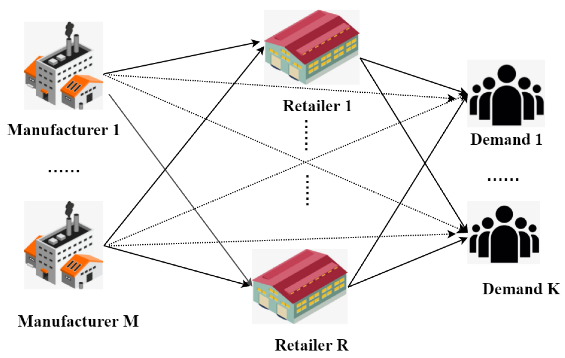
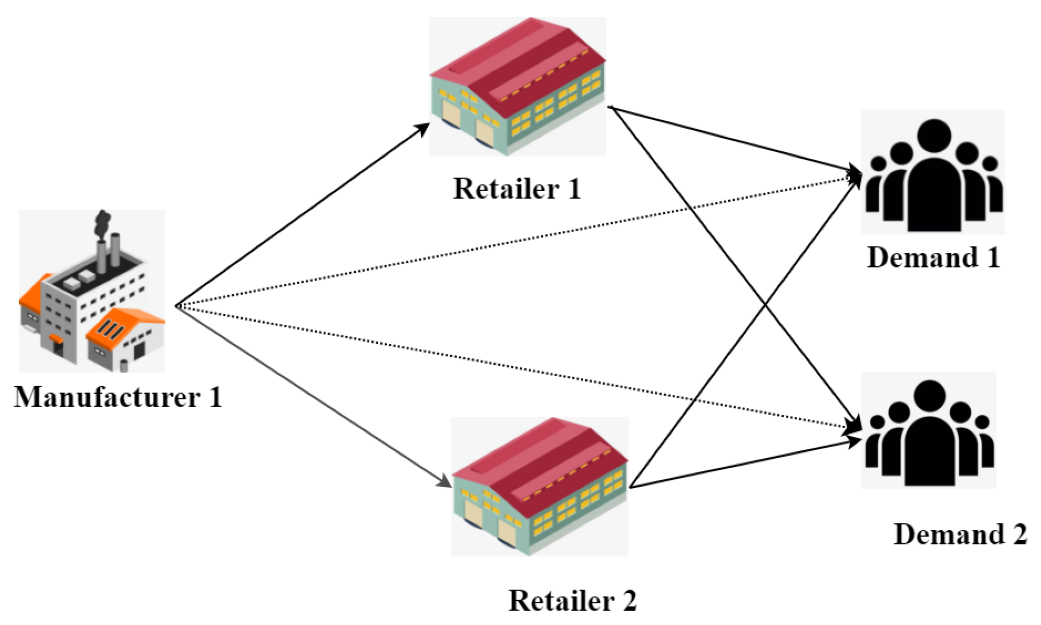
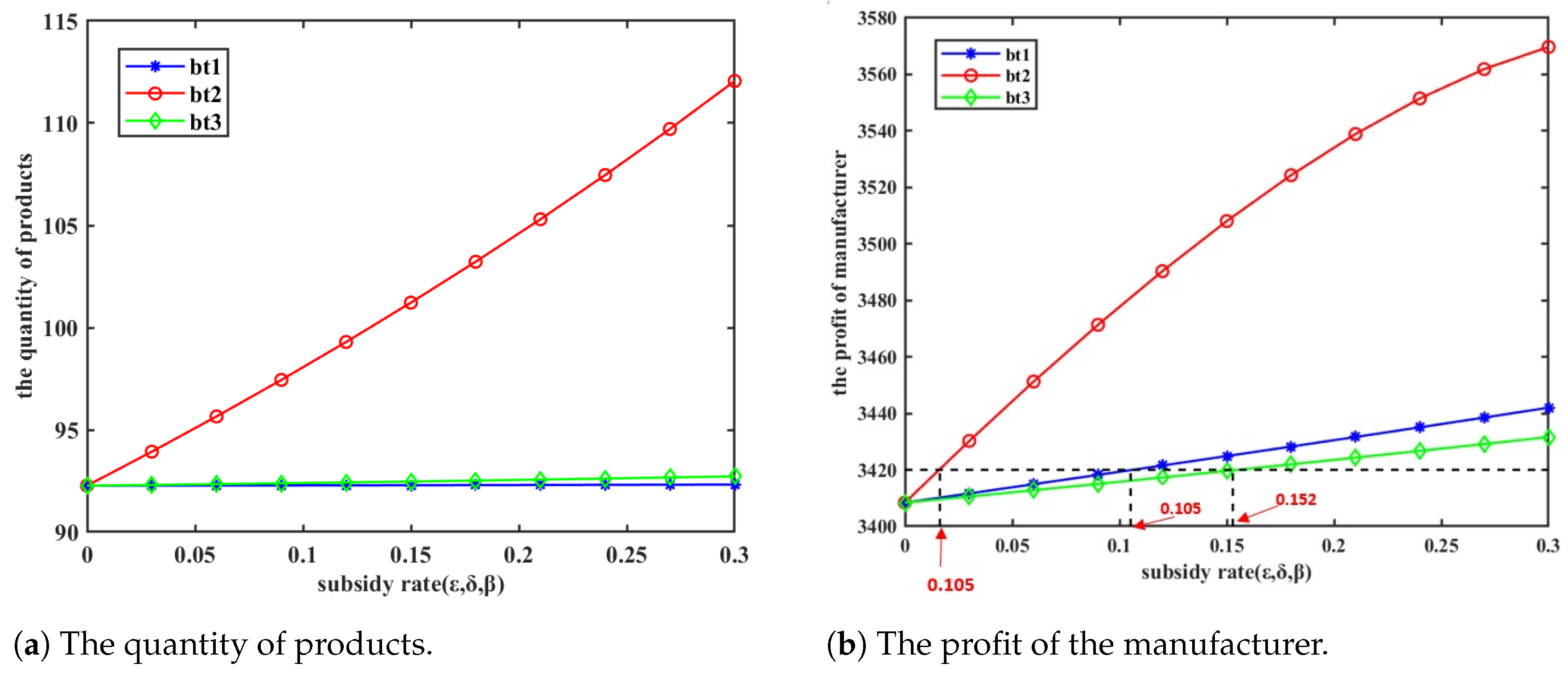
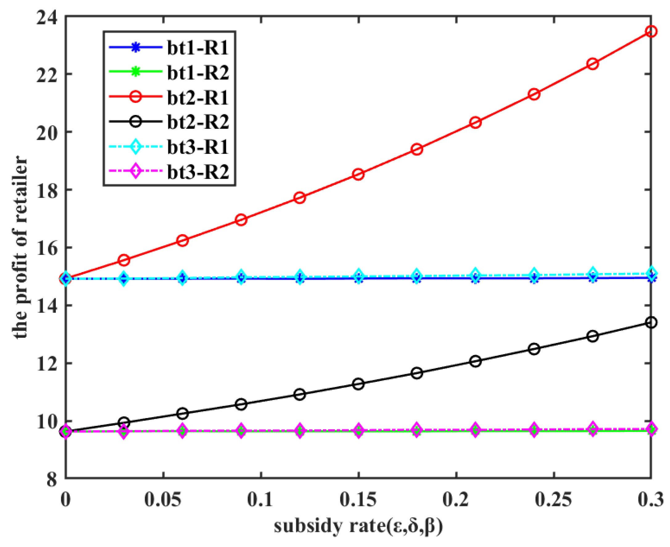
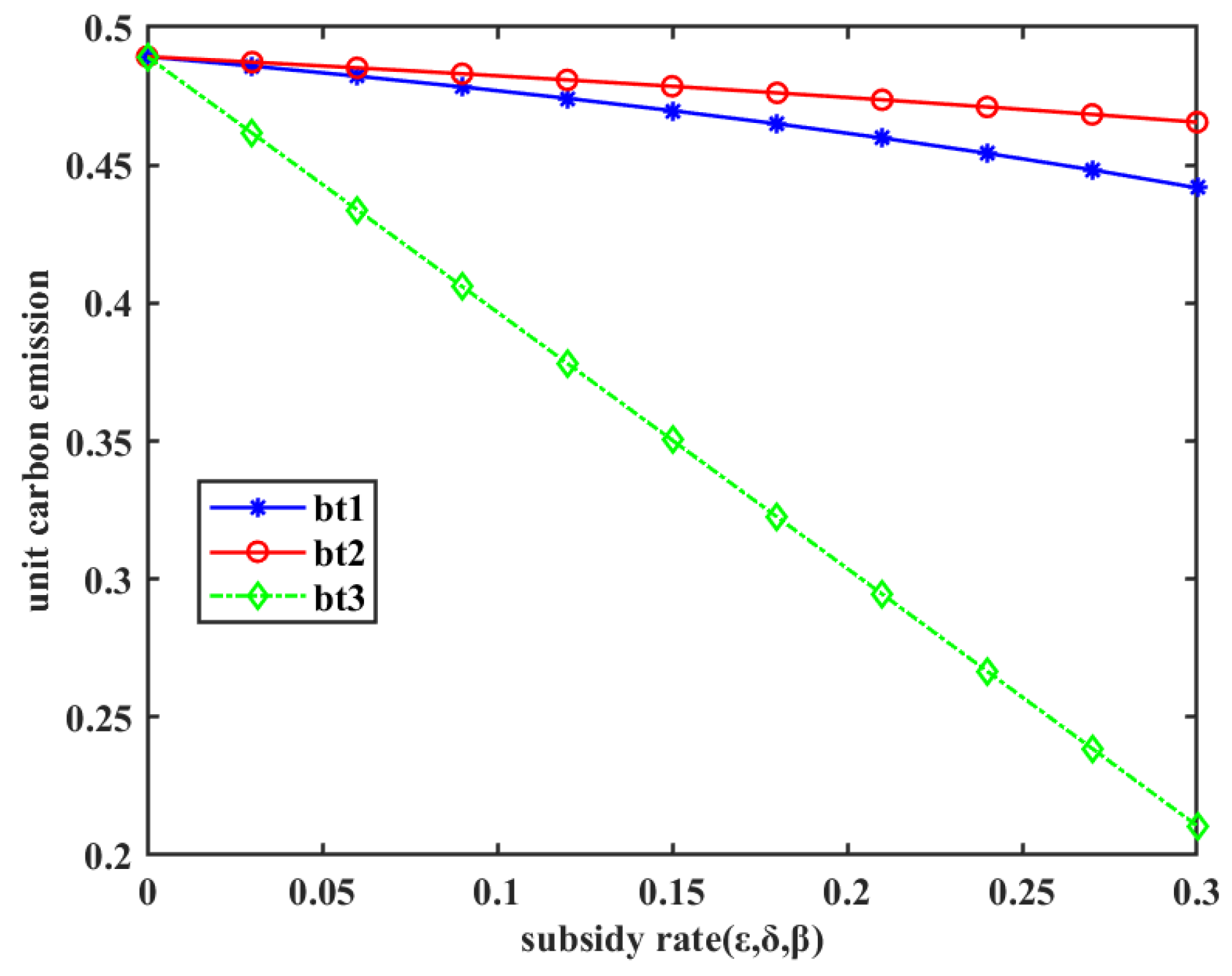

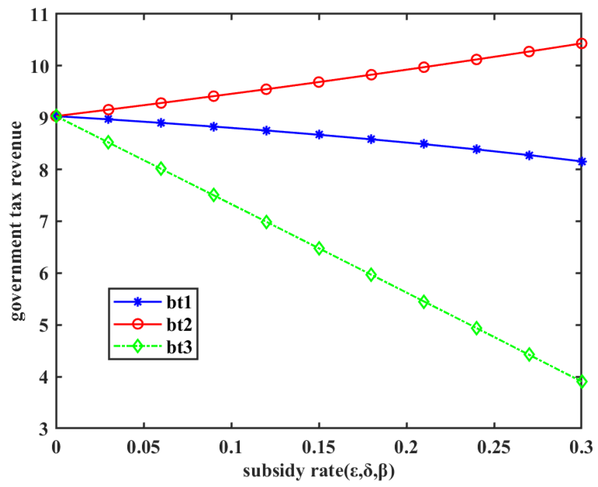
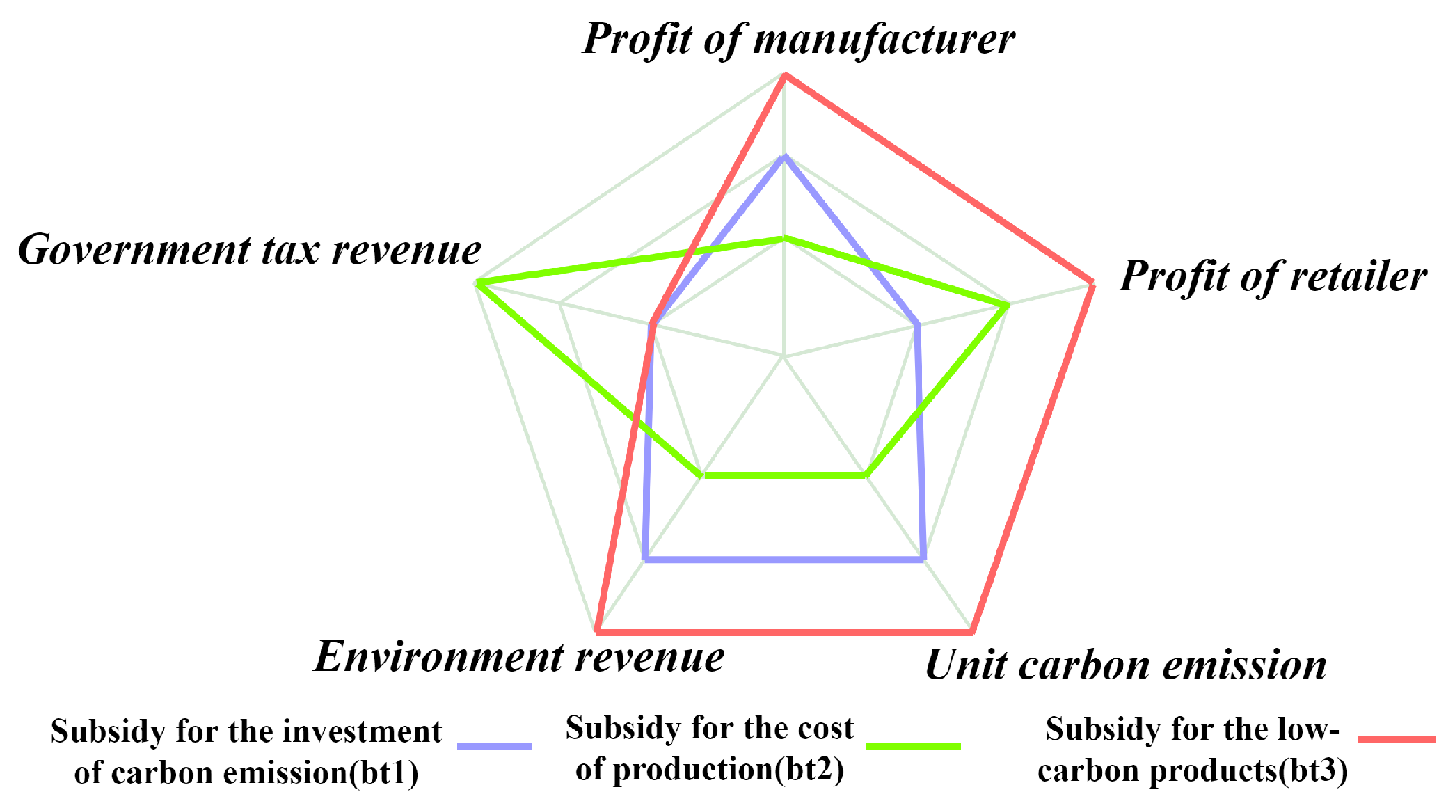
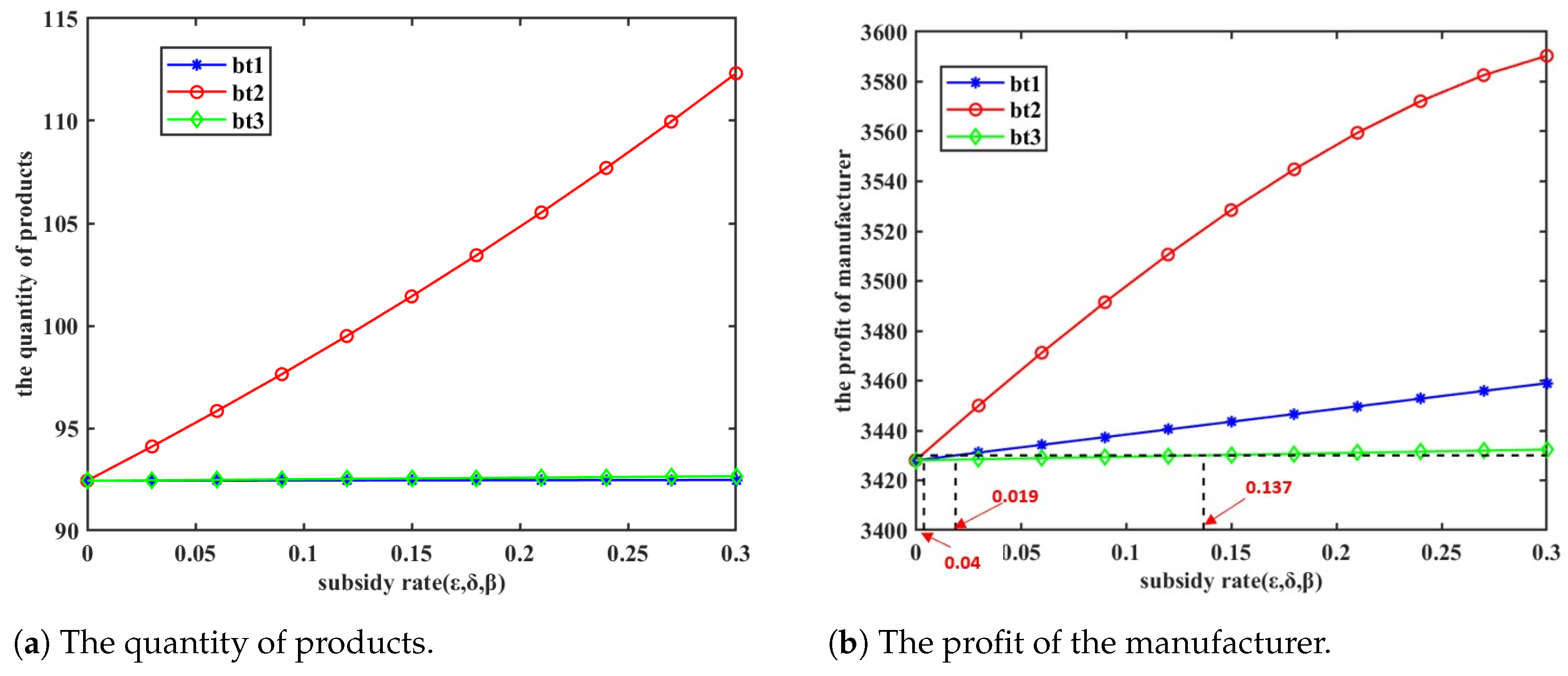
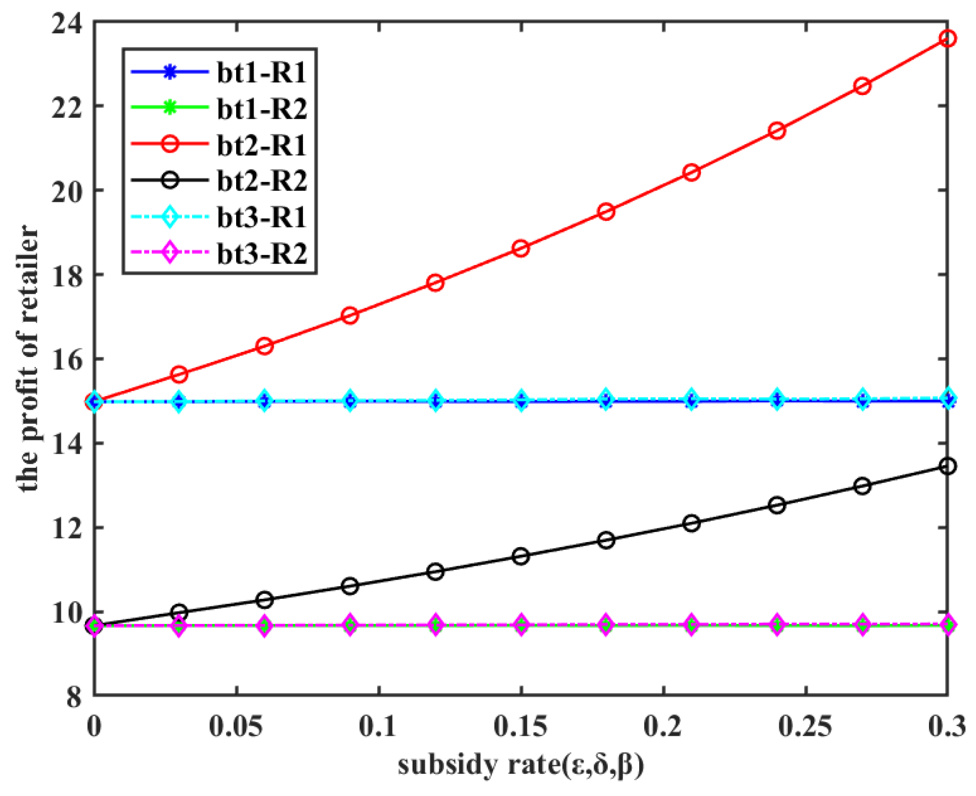
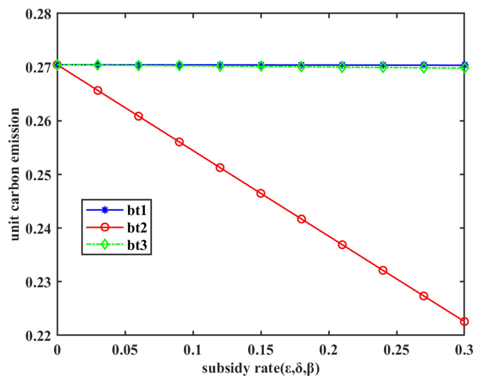
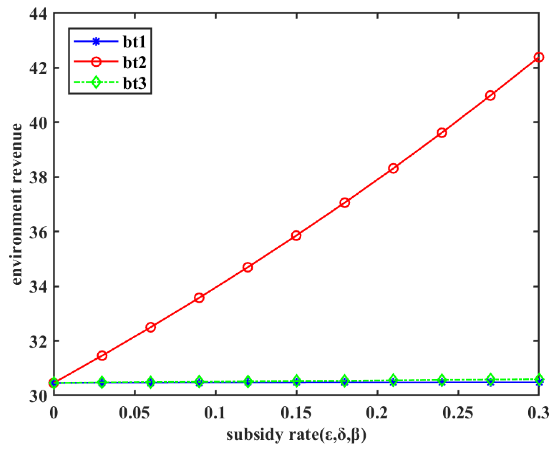
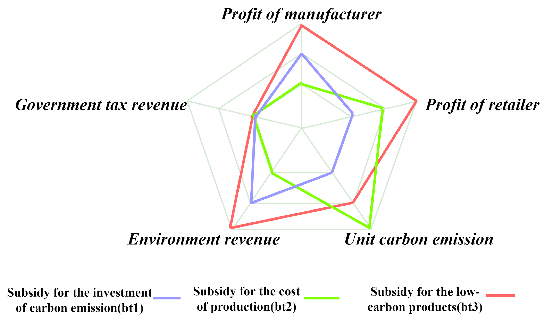
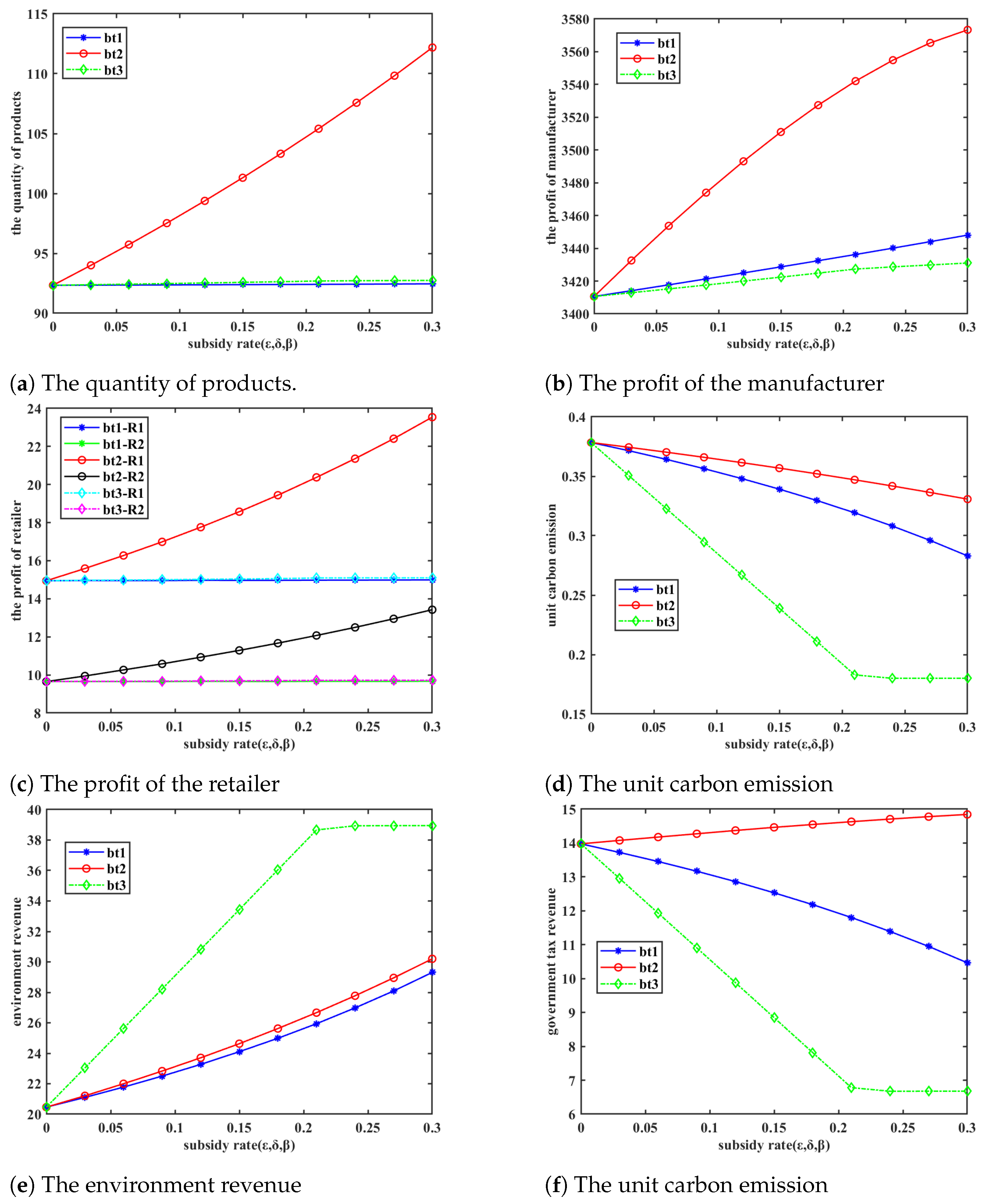
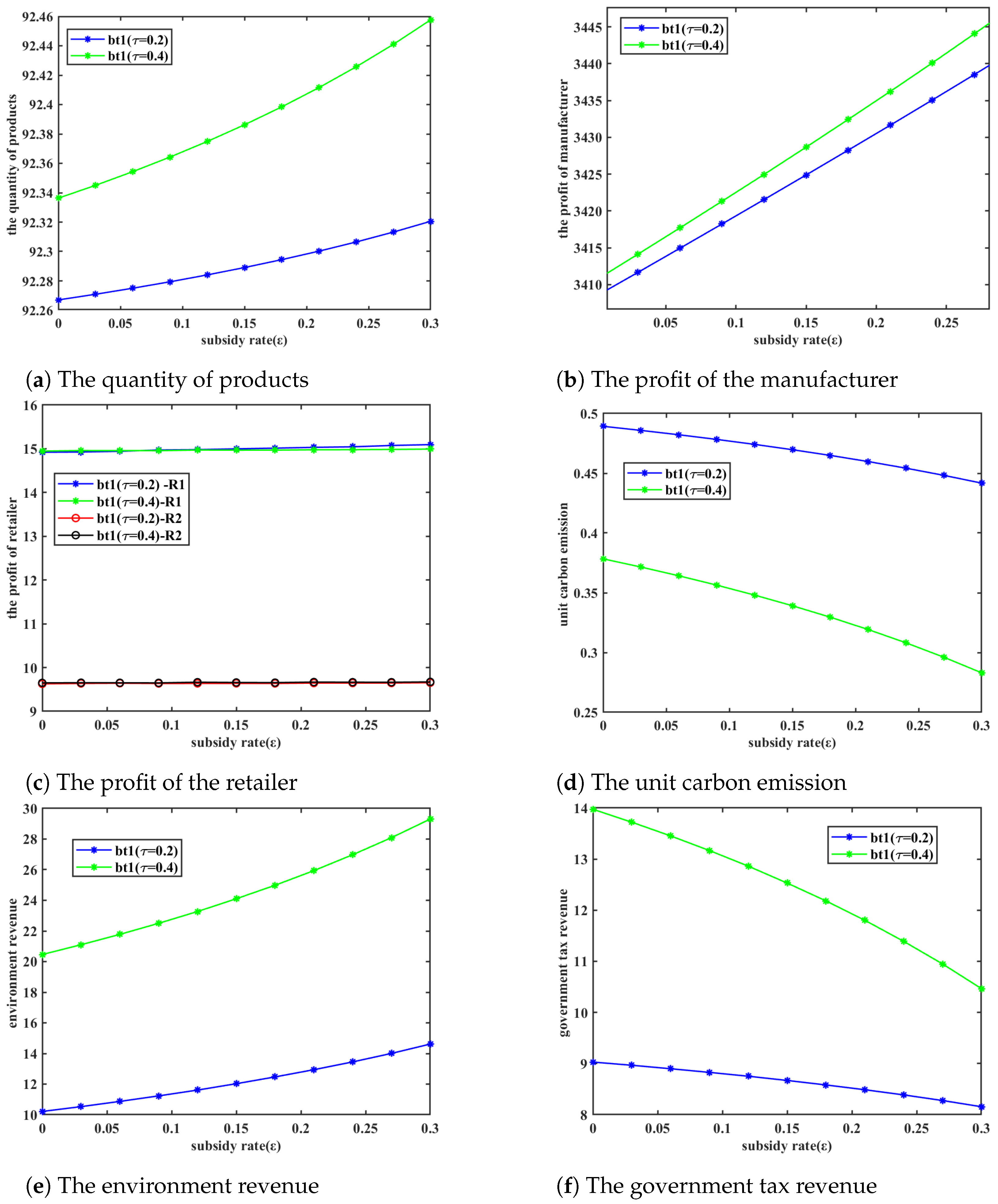
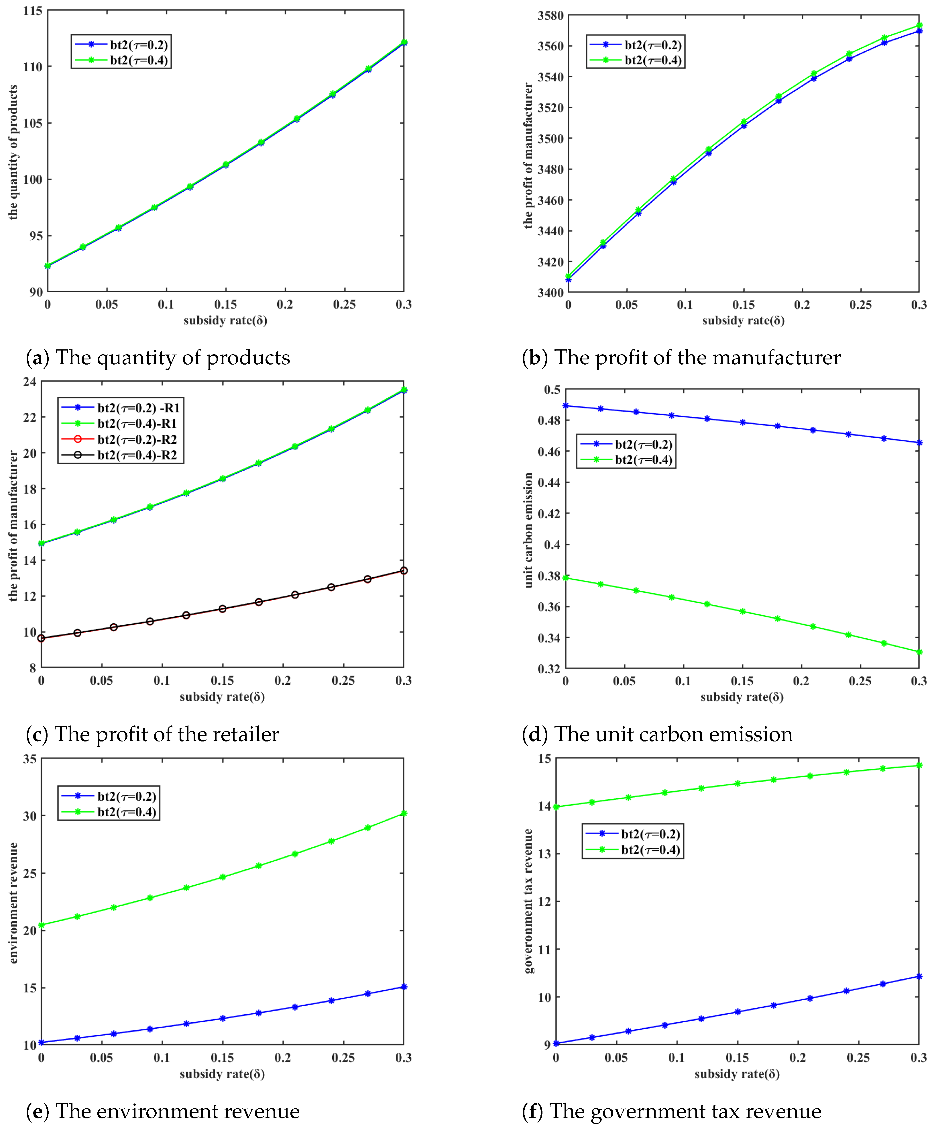
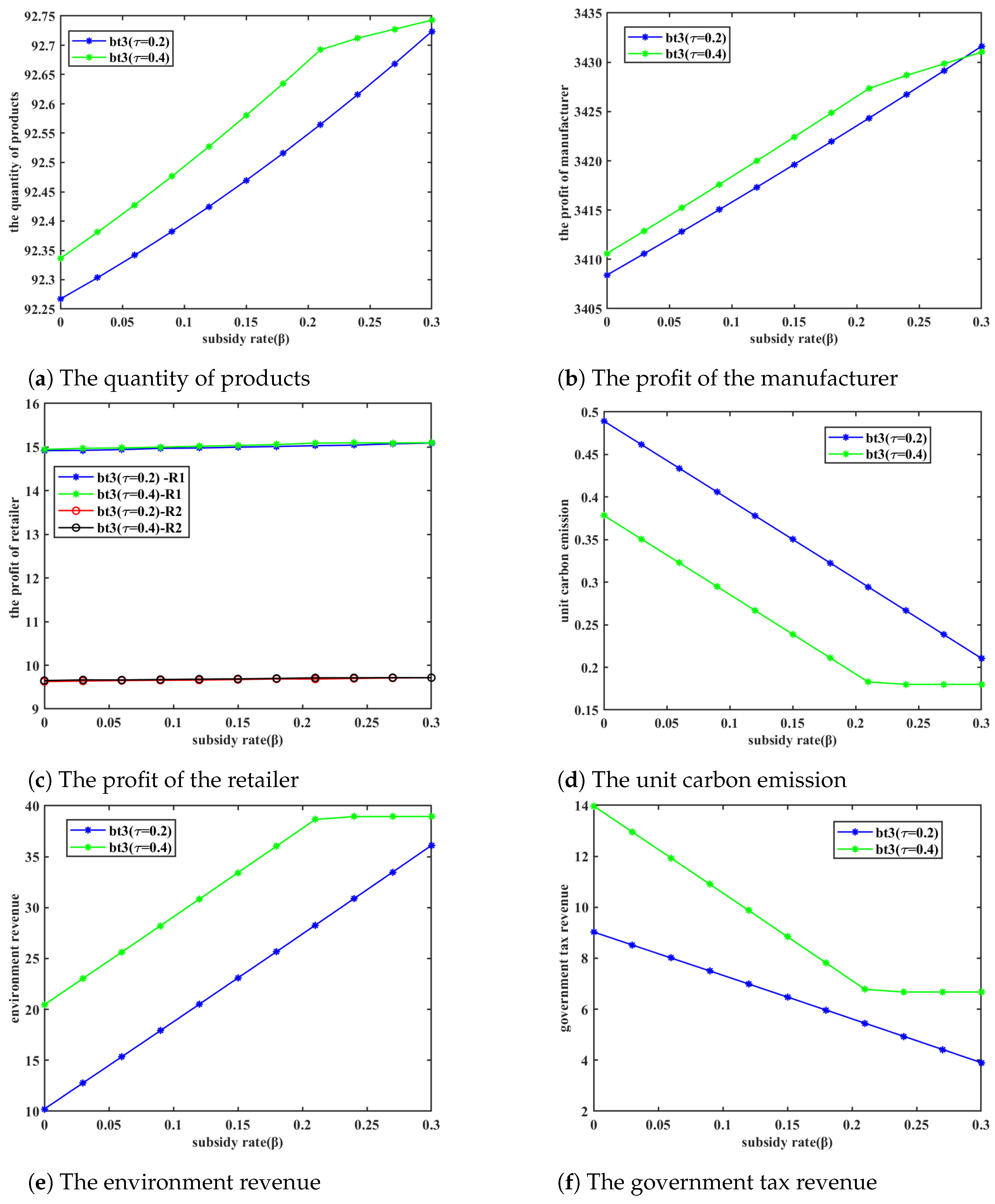
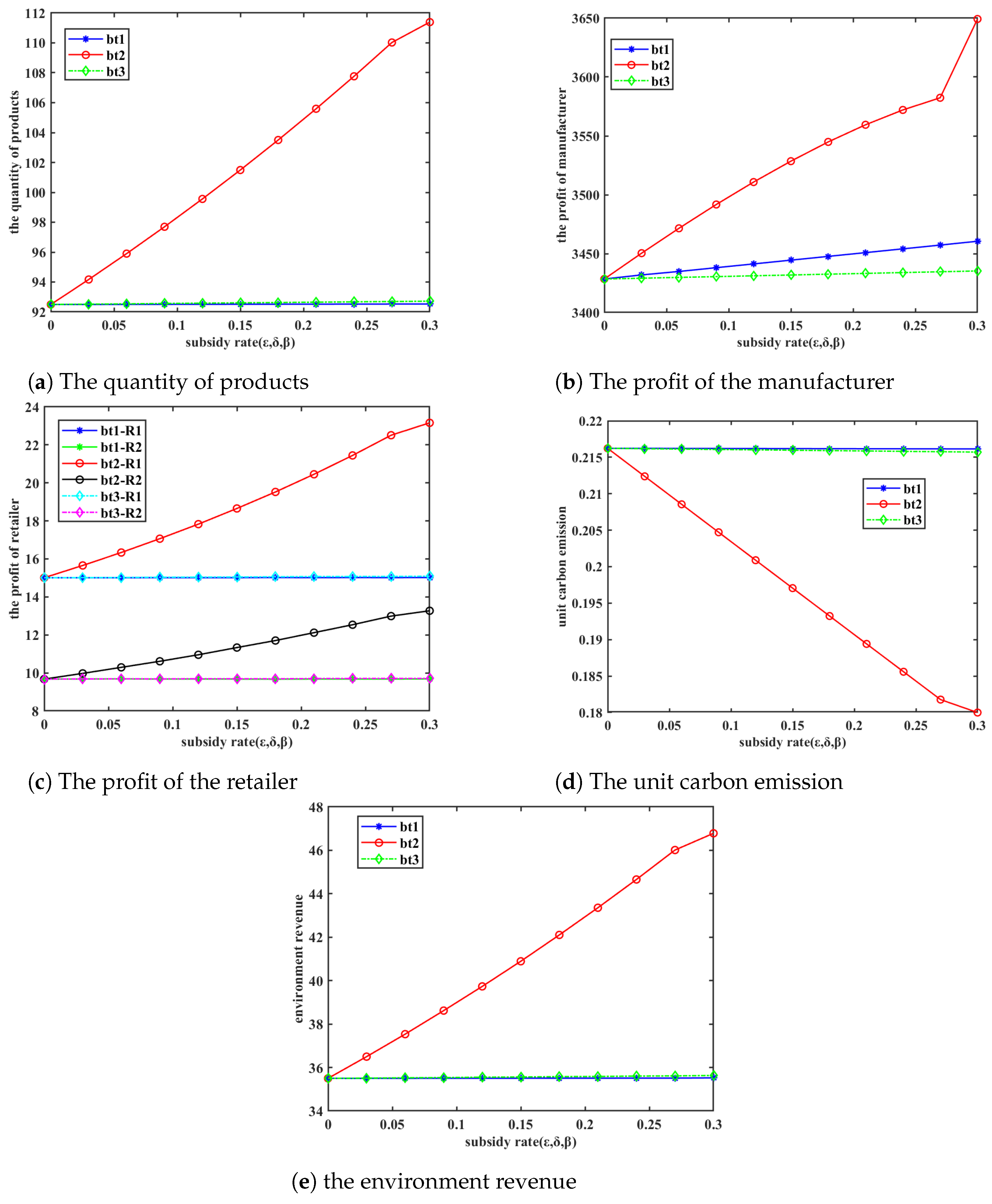
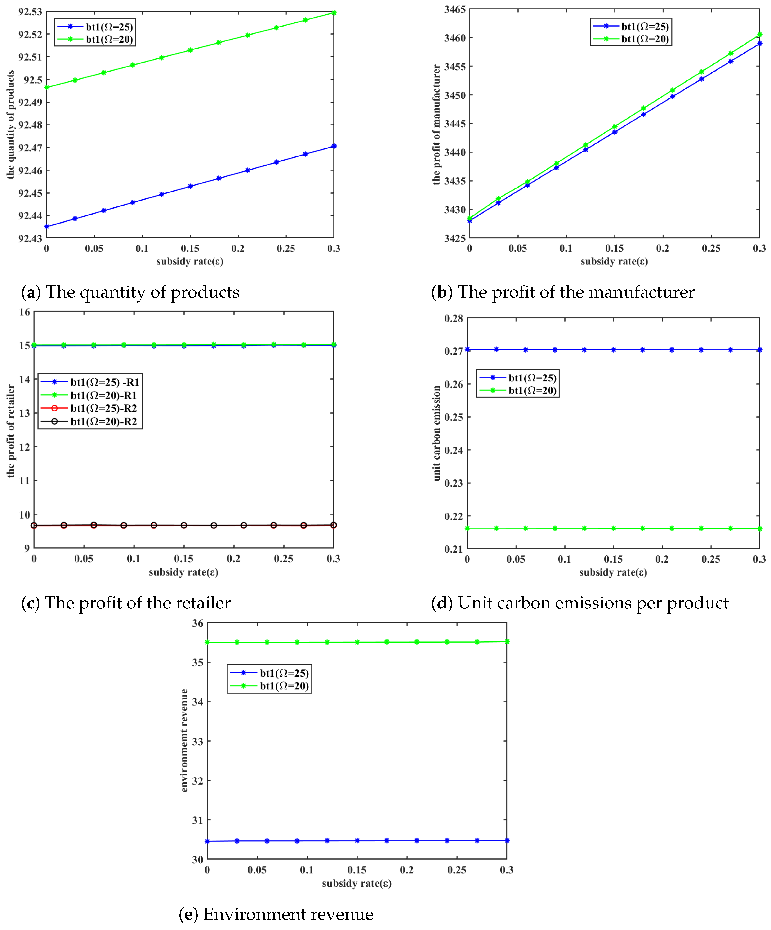
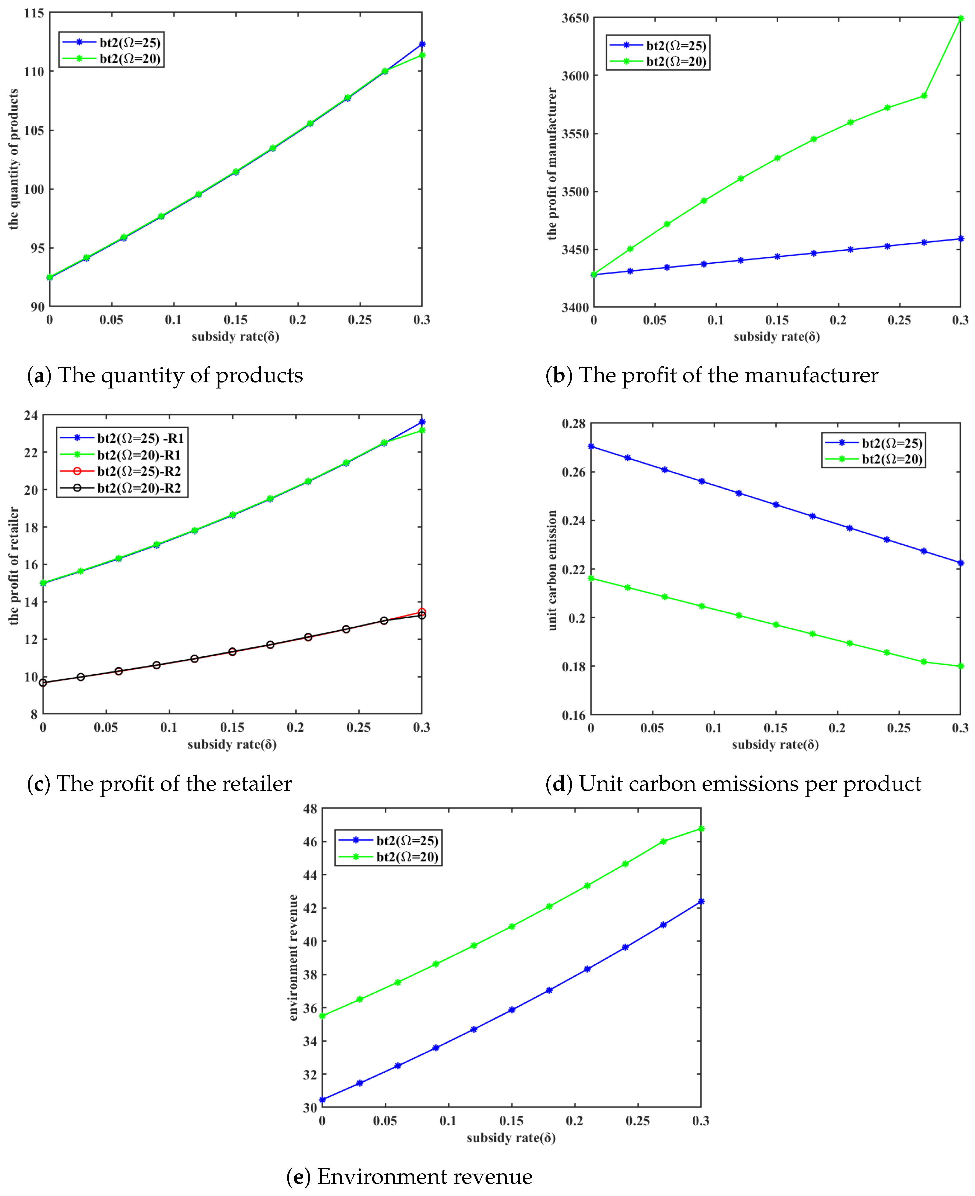
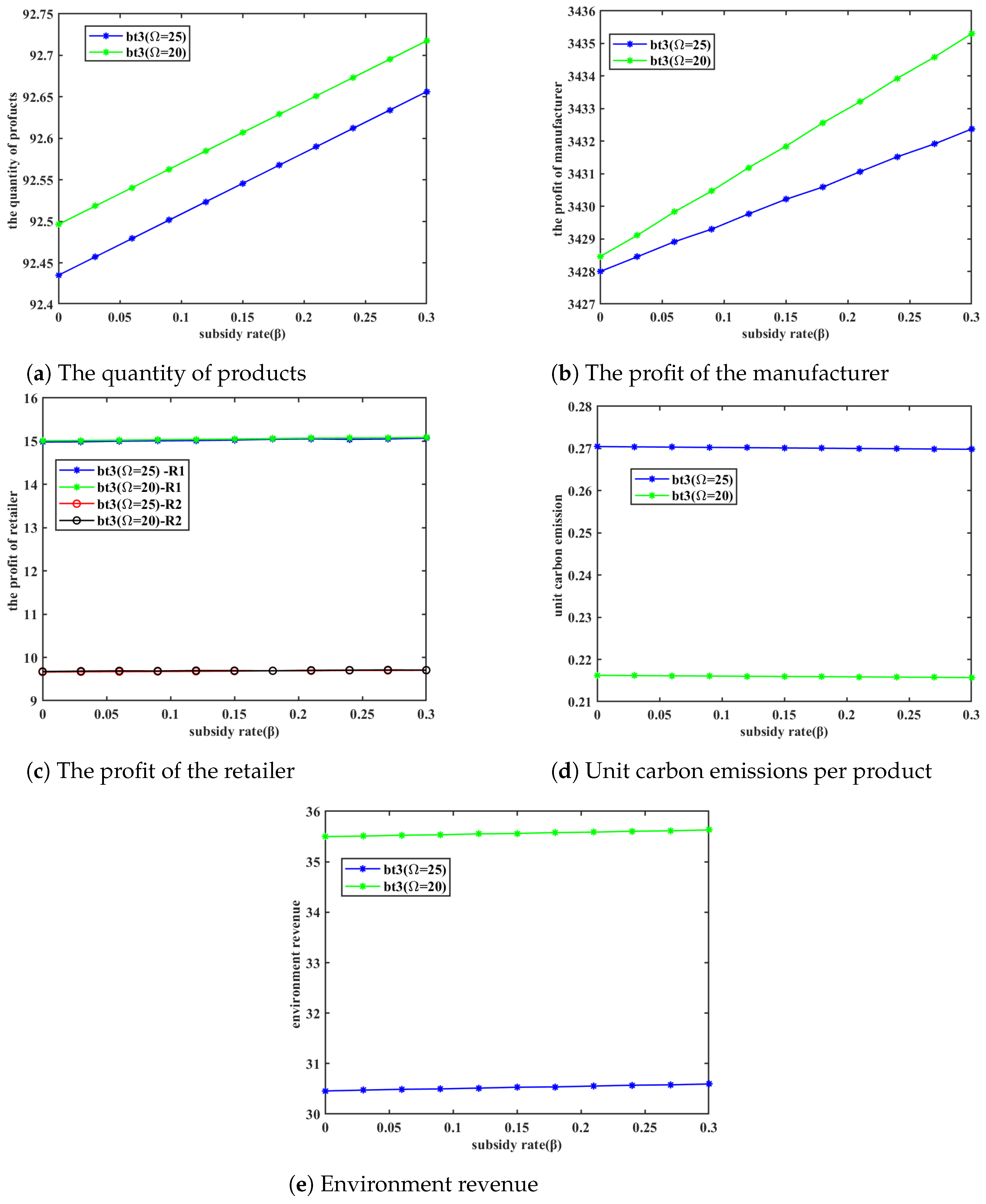
Disclaimer/Publisher’s Note: The statements, opinions and data contained in all publications are solely those of the individual author(s) and contributor(s) and not of MDPI and/or the editor(s). MDPI and/or the editor(s) disclaim responsibility for any injury to people or property resulting from any ideas, methods, instructions or products referred to in the content. |
© 2025 by the authors. Licensee MDPI, Basel, Switzerland. This article is an open access article distributed under the terms and conditions of the Creative Commons Attribution (CC BY) license (https://creativecommons.org/licenses/by/4.0/).